Submitted:
04 February 2025
Posted:
05 February 2025
Read the latest preprint version here
Abstract
In this work, we explore Conjecture 1 proposed in the newly released pioneering paper “Volatility transformers: an optimal transport-inspired approach to arbitrage-free shaping of implied volatility surfaces” by Zetocha Valer, which posits that the “One-X” property is both a necessary and sufficient condition for convex order between non-negative continuous strictly increasing distributions with the same mean. We provide a counterexample demonstrating that the conjecture, as originally stated, does not hold. By examining stochastic orders, particularly the increasing convex order, and the “One-X” property, we propose an enhanced version of the conjecture which is shown to be valid. Furthermore, we discuss the implications of these findings in the context of equity implied volatility fitting and the construction of implied volatility surfaces, highlighting the challenges posed by real-market conditions. In the end, we propose several applications in implied volatility surface construction or simulation. We also discussed the connection between TP2, RR2 and the one-X property.
Keywords:
Convex order
; "One-X" property
; imported volatility
; synthetic data generation
; stop-loss order
1. Introduction
Ever since the birth of Black-Sholes theory [6] and local volatility [9,10], construction of the implied volatility (IV) surface that is free of arbitrage has been an active research area. Although it may seem to be a simple task at the first glance, as pointed out in [29], constructing arbitrage-free IV surfaces that fit specific market conditions remains a challenging task for many sell-side institutions.
In a recent work [30] of Zetocha, an optimal transport-inspired approach has been introduced to understand the arbitrage-free shaping of IV surfaces. In this approach, a fundamental concept that mathematically describes the calendar no-arbitrage is the convex order “” : for random variables X and Y, we say if for any convex function , it holds
Given a set of random variables in convex order, i.e. (), they become the marginals of a martingale measure (thus free from calendar arbitrage); see Theorem 2.6 of [5] or Theorem 8 of [27]. It is therefore desirable to produce sequences of random variables that obey consecutive convex orders.
Notice however, that checking (1) for each and every single convex function is usually impossible in applications. A more natural and practical ordering between two random variables X and Y with the same mean is the so-called “One-X” order: we say if there is some such that
where and are the cumulative distribution functions (CDF’s) of X and Y, respectively. In this situation, the graphs of and intersects at the single point . Usually, by inspecting the graphs of the corresponding CDF’s, one could easily check the One-X order between a pair of random variables.
Besides the convenience, a key property mentioned in Theorem 3 of [30] (see also Lemma 2 of [23]) is that for random variables X and Y with the same mean, implies that . Moreover, the One-X order is preserved under the optimal transport maps generated from continuous and strictly increasing functions defined on ; for more detailed discussions see Section 6.2 of [30].
It is natural to guess whether these two orderings are actually equivalent: as asked by Conjecture 1 of [30], when and the CDF’s are both continuous and strictly increasing, is it true that implies ?
To answer this question, let us examine these concepts in a broader scope: both the convex order and the One-X order have their corresponding parts in the study of actuarial science, and their relations have been studied in the seminal work of [22]. In fact, unlike the convex order, the One-X order (or the dangerousness order in the language of actuarial science) is not necessarily transitive, and as shown in [22], it is the transitive closure “” of the One-X order that becomes equivalent to the convex order. We therefore expect a negative answer to the above mentioned conjecture. In the next section we will rigorously define the ordering concepts and summarize their relations. Then in Section 3 we will present a counterexample to Conjecture 1 of [30].
The rest of the paper devotes to discussing various conditions and methodologies on constructing IV surfaces that are free from both the butterfly arbitrage and the calendar arbitrage. We will focus on conditions that guarantee there to be no calendar arbitrage when working in the space of implied density functions, whose existence would already rule out the butterfly arbitrage.
In Section 4 we consider random variables with real-analytic CDF’s, and for each pair of such random variables with equal mean and in convex order, we prove the existence of finitely many consecutive One-X inequalities interpolating between them (Theorem 2) .
In Section 5 we will discuss how the One-X property could be deduced from several important concepts such as totally positive of order 2 (), reverse rule of order 2 (), and unimodality of density ratios, which are introduced to the study of convex ordering through the seminal work [24] and [25].
The last section is devoted to a general discussion on several aspects of the IV surface construction and highlight a novel approach: we propose to apply the martingale interpolation techniques to the construction of the intermediate implied density functions at maturities with poor liquidity; we will also discuss a framework of synthetic IV generation that harnesses the power of machine learning.
2. Background
In this section, we will first recall the definitions and properties of some well-known stochastic orders between one-dimensional random variables, which will be used intensively in the later sections. Then we will introduce the dangerousness and the One-X property which enable us to state and understand the meaning of the conjecture in [30].
2.1. Stochastic Orders and Their Properties
In this section we present rigorous mathematical definitions of the related stochastic orders, as well as some useful properties. We assume that there are two random variables X and Y with CDF’s and respectively.
Definition 1.
X is smaller than Y in the increasing convex order, denoted as , if for any real-valued increasing convex function f,
provided both expectations exist.
Since any increasing convex function can be obtained as the limit of linear combinations of the functions in the form , , (3) in the above definition can be replaced by
Using integration by parts it is also easy to show that (4) is equivalent to the following integral inequality of their corresponding CDF’s:
If we replace increasing convex function by convex function, then X is called smaller than Y in convex order, denoted as ; recall (1). When , one can show that these two orders are equivalent, i.e. ; see Theorem 4.A.35 of [26] for more details. Under the assumption that , we can therefore use these two definitions in an exchangeable manner.
Lemma 1
(Theorem 2.3.10 [3]). Let X and Y be two random variables. Then if and only if for all real valued increasing convex function ϕ.
In particular, as multiplication by a positive constant is an increasing convex function, we have
Lemma 2
We therefore have the following useful corollary for the construction of the counterexample:
Corollary 1.
Given two sets of independent random variables and such that for all . If are positive numbers, then
2.2. One-X Order and A Related Conjecture
To recall the One-X order defined in (2), we start with the more general definition of the dangerousness ordering which has been introduced to the study of the actuarial science by [22].
Definition 2.
Given non-negative one-dimensional random variables X and Y whose CDF’s are and respectively, X is called less dangerous than Y, denoted by , if there exists some such that over , over , and .
When is required, this relation is called One-X in [30]; in this case we will write .
As mentioned before, we have the following implication:
Theorem 1
(Theorem 3 of [30]). Given non-negative one-dimensional random variables X and Y such that , then .
The inverse to this theorem is conjectured by Zetocha: [Conjecture 1 of [30] Given non-negative one-dimensional random variables X and Y whose CDF’s are and respectively. Suppose and are continuous and strictly increasing functions on , and , then .
By providing a counterexample to this conjecture in the next section, will show that a single One-X inequality is not enough for a pair of random variables satisfying the convex ordering.
2.3. Inter-disciplinary Concept Comparison
Till now, we have seen several orderings such as the convex order, the One-X order, and the dangerousness order. Some of these concepts occur in financial mathematics, and some of them originates from actuarial science. In this subsection we will try to make a more systematic summary of these concepts and some results, aiming to build a dictionary between some of the important concepts from the two fields.
For the sake of simplicity, we will work under the assumption that all the distributions are non-negative, continuous and with the same mean. Given two random variables X and Y with continuous, strictly increasing CDF’s and the same mean, the following table briefly summarizes the various orderings in different contexts:
| Financial Mathematics Concepts | Actuarial Science Concepts |
| One-X Order: | Less Dangerous: |
| Increasing Convex Order: | Stop-loss Order: |
| Convex Order: | Transitive closure of : . |
In each of the first two rows, the concepts are mathematically defined in identical manners. The two concepts in the third row are shown to be equivalent by Corollary 4.4 [22]. Moreover, the lack of transitivity of or makes them inequivalent to , and their transitive closure is defined as following: if there is a sequence of random variables such that , and that weakly. Notice that under the assumption , it consequently holds that for all .
3. A Counterexample to Conjecture Section 2.2
In this section, we begin with reviewing some conditions on the existence of (increasing) convex-order between two distributions belonging to some specific exponential families. We will then construct two random variables with the same finite mean that are in convex order; moreover, they have continuous and strictly increasing CDF’s, but their CDF’s cross more than once: this violates the corresponding One-X inequality and becomes a counterexample to Conjecture Section 2.2.
3.1. (Increasing) Convex Order Between Exponential Family Distributions
We will consider the Gamma and the Weibull distributions. Conditions on the existence of increasing convex order between two given Gamma or Weibull distributions are given following their definitions. We follow [3] for the notations and the main results in this part.
Definition 3.(Gamma Distribution) A non-negative continuous one-dimensional random variable X follows the Gamma distribution, denoted by , if its probability density function (PDF) is given by
where is called shape parameter, is called scale parameter.
If , then .
Definition 4
(Weibull Distribution). A non-negative continuous one-dimensional random variable X follows the Weibull distribution, denoted by , if its CDF is given by
where is called scale parameter, is called shape parameter.
If , then .
Given two random variables which follow either the Gamma or the Weibull distributions, let’s state some sufficient conditions to guarantee the existence of increasing convex order relation between them. These sufficient conditions are adopted from Section 2.9.1 of [3] :
Lemma 3.
Given two random variables , if and , then . If , then .
Given , if and , then . If , then .
Here we rely on the fact that if two non-negative random variables with the same mean follow increasing convex order, then they are in convex order; see Theorem 4.A.35 of [26].
3.2. The Counterexample
We consider the following random variables with the same mean:
where the six independent random variables are
- , , ;
- , , .
By Lemma 3, it is clear that , for the two pairs of Gamma distributions, and each pair share the same mean. For the pair of Weibull distributions and , notice that ; moreover, since and , it follows
Therefore by Lemma 3. Since () are positive linear combinations of ’s, we have by Corollary 1.
We can also plot the CDF’s of each pair of and (), and their CDF’s satisfy the One-X inequality for each j. According to Theorem 3 of [30], we can therefore conclude that for each ; this is consistent with our analysis above. The plots of each pair of CDF’s can be seen in Figure 1.
To conclude our argument on this counterexample, let us plot the CDF’s of probability distributions and in Figure 2, where we can easily see that they intersect more than once, as we can numerically check that
but on the other hand
Therefore , but we have already shown that . This completes the counterexample.
4. One-X Interpolation Between Convex Ordered Pairs
Although Conjecture Section 2.2 fails in the most general scenario, we may focus on smaller classes of distributions and obtain a partial inverse to the implication “”. Before determining which classes of distributions are viable in practice, let us discuss a general result.
4.1. A General One-X Interpolation Result
As mentioned in Section 2.3, the One-X order (or the dangerousness order) is not transitive, and its transitive closure requires inserting extra terms in between two random variables satisfying the convex order. Theoretically there might be infinitely many intermediate terms appearing.
From a practical point of view, we are mainly interested in pairs of random variables that satisfy the following assumptions:
- The random variables assume positive value, since they reflect the distributions of tradable assets on different expirations, and thus they are positive in nature.
-
The random variables share the same mean, since in the most intriguing cases the underlying assets behave as martingales after certain preparation.When the underlying is of equity class, the existence of dividends brings challenges into the construction of IV and local volatility surface. One way to bypass this is the pure stock process [8]: assume that the equity price is , the pure stock is defined as where and is the stock’s forward price. As shown in [8], is a positive martingale with , and all the pricing theories can be transformed from to . In particular, the construction of IV surface or the implied density will be associated with the process.When the underlying is of fixed-income class, the typical options are caps/floors and swaptions. For caps/floors, the underlying is the forward rate which is a martingale under T-forward measure; for swaptions, the underlying is the swap rate which is a martingale under swap measure (for more technical details, see [1]).
- The CDF’s of the random variables are analytic functions, as they mostly arise from approximations of market data by known families of analytic distributions.
For random variables satisfying the above mentioned assumptions, we have the following finite intersection result.
Proposition 1.
Given two random variables () whose CDF’s, denoted by respectively, are defined on , if their CDF’s are real-analytic, then the number of intersections of and is at most countable, and is finite on bounded intervals. If we further assume that the density function of dominates that of , then there are finitely many intersections.
Proof.
We begin with covering by . Define , h is also analytical whose zero points correspond to the intersection numbers of and . Let’s show that over each sub-interval , h has finitely many zeros, thus, it has at most countably many zeros. is a compact set in . If h has infinitely many zeros, then by Bolzano-Weierstrass Theorem, the set of zeros has a convergent sub-sequence in . Therefore, by identity theorem, h must be zero on all of which implied h is identically zero. This is a contradiction to the assumption that and are different.
Let’s denote the density functions by , . If dominates , then . Thus, there exists a positive number A such that and intersects at most once over . Following the same argument as above, we can show that and only intersect finite many times over . Thus, if dominates , their CDF’s have only finitely many intersection points. □
Remark 1.
In Proposition 1, we prove the result under the general assumption that the CDF/PDF of the random variables are real-analytic, and the proof is from scratch. As discussed below in Section 4.2, we are more interested in the special case in which the density functions are log Gaussian mixtures, and in this case, the conclusion of this proposition follows from Proposition 4.1 in [13] 1.
From the above discussions, we can see that the our above assumptions are quite natural yet still can largely cover the cases one can meet in practice. Now, we are ready to state and prove the following theorem which is one of the main results of this paper:
Theorem 2.
Given two non-negative one-dimensional random variables X and Y which share the same mean, and their CDF’s, and , cross finitely many times (say, n times), then if and only if there exists a sequence of random variables such that , , and for .
Proof.
The if part is relatively straight forward. By Theorem 3 of [30], the One-X order implies the convex order. Thus, for any , implies that and . These two properties are both transitive, and thus . (Notice that if one fixes n as 2, then this is the original conjecture).
Now, let us prove the only if part. By Theorem III.1.3 of [19] or Theorem 1.1, Chapter IV of [18], and n intersections of the CDF’s implies that there exists a sequence of random variables such that , , , for . By Definition 1, this implies ; however, notice that , and thus, all the random variables in this sequence share the same mean which shows that , for . □
Remark 2.
When and cross possibly infinitely many times, one needs to replace the finite sequence in Theorem 2 by a possibly infinite sequence which convergences to Y in both distribution and mean (which is called “stop-loss convergence"). A proof of this generalization can be found in Section 4 of [22]; compare also the transitive closure of the dangerousness order mentioned in Section 2.3. An example when there are infinitely many intersections is given below. note1
Example 1.
An example where there are infinitely many intersections can be found in [13]. Assume that X is a log normal random variable whose density function is
random varible Y, introduced by Heyde, is defined to have a density function
then their CDF’s of X and Y have infinitely many intersections.
4.2. Log Gaussian Mixtures
There are several very popular IV surface construction methods, besides the well-known parametric method such as stochastic volatility inspired IV surface [12], another major approach is through the construction of implied density per time-slice. One benefit of this method is that the existence of implied density function implies no butterfly arbitrage automatically. Consequently, the main challenge remains to deal with the calendar arbitrage, for which the existence of One-X orders will play a key role.
Notice that the implied density in [30] obeys log normal distribution. This assumption helps to explain the theoretical foundations explicitly and facilitates the implementation of the proposed IV surface construction method. However, as pointed out in [13], a single log normal distribution alone suffers the difficulty of fitting the IV smile in the real market, especially before the companies’ earning dates when the implied volatility smile may become W-shape. Therefore, we propose to use mixtures of log normal distributions (aka log Gaussian mixtures) to fit the implied density functions. The rational of this proposal is also based on the fact that Gaussian mixtures are weakly dense in the set of probability distributions; see Page 65 of [14].
Directly combining Theorem 2 and Proposition 1 (see also Proposition 4.1 in [13]), we have the following result for log Gaussian mixtures:
Theorem 3.
Given two random variables X and Y whose distributions are log Gaussian mixtures; suppose , then if and only if there exists a sequence of random variables such that , , and for .
In Section 6, we will further elaborate on the convex ordering of log Gaussian mixtures concerning the construction of IV surface.
5. , , Unimodality of Density Ratio and Convex Ordering
As mentioned in the introduction, it has been an active research area to understand various conditions which guarantee that there is no calendar arbitrage between two given marginal densities. In the recent work [24] and [25], concepts such as , and unimodality of density ratio have been introduced to the field. In particular, various sufficient conditions for the existence of convex order between given marginal densities have been discovered based on the information associated with these concepts. In this section, we study how similarly proposed conditions can lead to the more geometrically intuitive One-X property which is stronger than (and thus implies) the the convex ordering.
5.1. A Brief Review of the Concepts
We begin with recalling the definitions and key properties.
()).
Definition 5 (Total Positivity of Order 2 Let be a function defined over the product of intervals . If it holds
then is called totally positive of order 2, denoted as .
()).
Definition 6 (Reverse Rule of Order 2 Let be a function defined over the product of intervals . If it holds
then is called reverse rule of order 2, denoted as .
These two concepts are obviously in some form of duality, as one sees from the following criteria for and :
Proposition 2.
Assume that for all . Then
-
is is increasing in y, for any fixed , andis is decreasing in y, for any fixed ;
-
if is differentiable in x, thenis is increasing in y, andis is decreasing in y;
-
if is, moreover, twice differentiable, thenis , andis .
These properties are well-known and can be easily verified by elementary calculations; see also Section 2.1 of [25].
Definition 7
(Unimodality of Density Ratio). Assume that there are two non-negative random variables and with the same mean, and that their PDF’s () are continuous and positive on the interval , where we denote and . We call and satisfy the unimodality of density ratio if there exists such that the ratio is increasing in x over , and decreasing over .
In real world applications, and are the marginals of the underlying with and , where denote the time-to-maturity. In consideration with option pricing the following result in Sectioin 3 of [25] is useful:
Proposition 3
(Corollary 3.1 of [25]). Given a non-negative underlying process , and assume that the marginals and ( denoting the time-to-maturity) have the same mean. If and satisfy the unimodality of density ratio, then
- is increasing for , and
- is decreasing for ,
where (resp. ) denotes the call (resp. put) option price with strike and riskless rate .
Now considering the setting of the above proposition, if the underlying process is continuously and non-negatively defined for , we see that for any , is a continuous function, and thus is well-defined for any . Therefore, we can define, for the process , the quantities
For this process we let denote the PDF of the marginal distribution induced by , and it is obvious that . In order to describe such functions by properties like total positivity or reverse order, we introduce the following
Definition 8.
We say that defined on is mixed then if there is some such that is on and it is on .
We can also consider a strengthened version of unimodality of density ratio for a continuous family of PDF’s in the follwing
Definition 9.
Given a continuous process with marginal PDF defined on , we say satisfies the uniform unimodality of density ratio condition if there is some such that for any with , the function is increasing in and decreasing in .
We have the following characterization as a consequence of Proposition 2:
Proposition 4.
Given a continuous non-negative underlying process defined on and assume that , the PDF of , is differentiable in x, then the following are equivalent:
- satisfies the uniform unimodality of density ratio; and
- is mixed then on .
Proof.
For any such that , we calculate the following thanks to the positivity of the marginal PDF’s:
Therefore, the function is increasing for for some if and only if the function is decreasing for each fixed (as a parameter), and the function is decreasing for if and only if the function is increasing for each fixed (as a parameter). By Item (2) of Proposition 2 it is clear that satisfies the uniform unimodality of density ratio if and only if is then on . □
Remark 3.
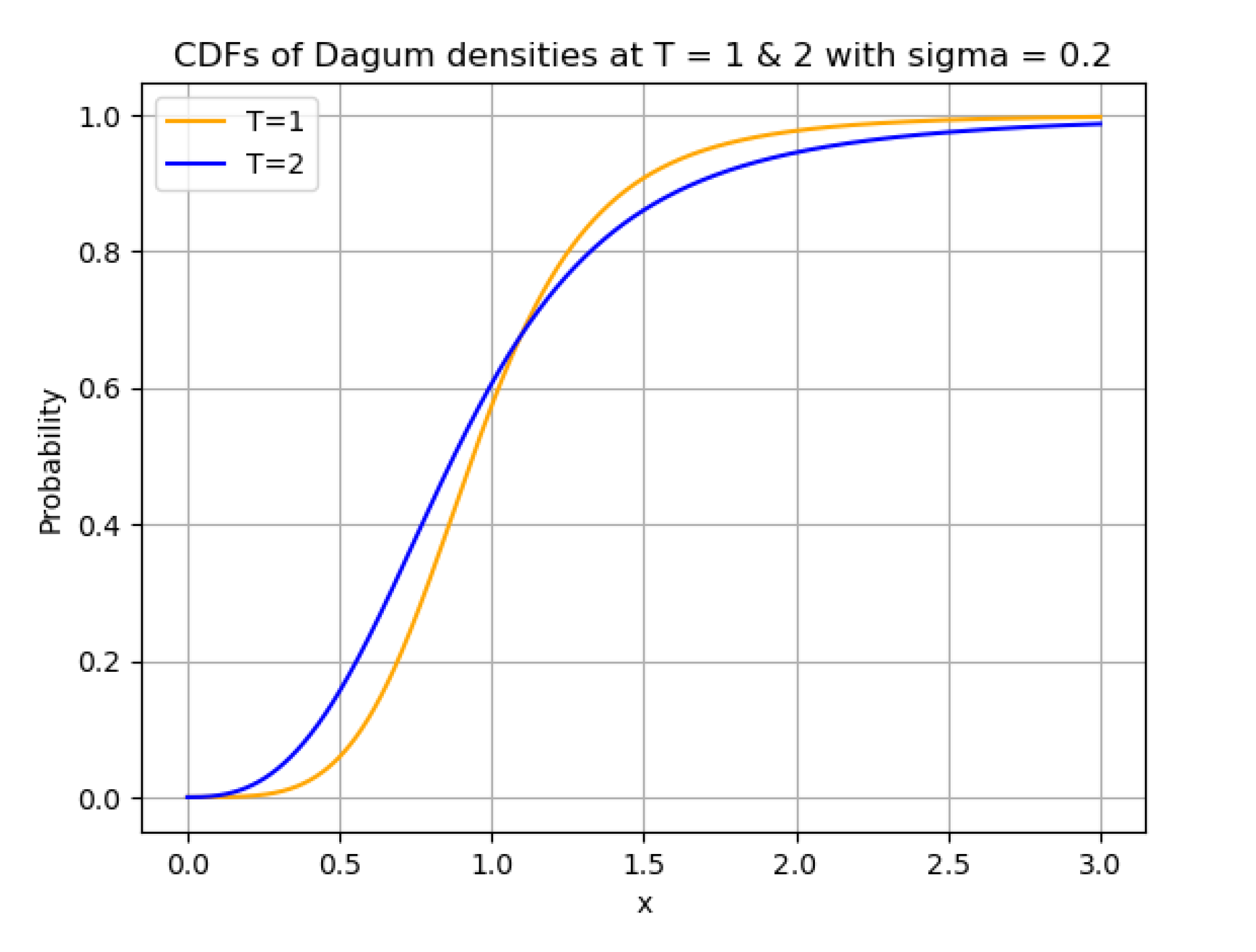
Although it seems that the characterization of the mixed then condition is quite restrictive by assuming afixed that does not change with different pairs of time-slices, such a situation do occur in several natural instances, such as the log Gaussian mixture with the same mean in Lemma 3.1 of [24], the scalar diffusion in Section 4.1 of [24], and the Dagum density in Section 4.6 of [24].
5.2. Relation with the One-X Property
Here we emphasize that instead of directly proving the existence of convex ordering out of the above reviewed conditions, we notice that they actually imply the stronger ordering, the One-X property between marginal CDF’s. Firstly, considering the unimodality of density ratio, we have the following result.
Proposition 5.
Assume that and satisfy the unimodality of density ratio and that , then and satisfy the One-X property, and thus .
Proof.
From the definition we have , and there exists such that the ratio is increasing in x over and decreasing over , where denotes the PDF’s of respectively for .
Rename with , and set . Then
Since increases on , decreases on and , we have
Since for , we have
and denoting (), we have
In the notation of [3], this exactly means that . By Theorem 2.3.8 of [3], we thus have with sign when equality holds.
Since , if then it holds according to Theorem 3.A.44 of [26]. Moreover, since is mainly considered as some underlying asset, we may assume in practice. Consequently, implies that .
We therefore only need to show that the number of intersections :
- If , there is no intersection between the graphs of and of . Without loss of generality, assuming on , we would arrive at the following contradictionsince .
- If , then the graphs of and intersects at a single point , with signs or . In either cases, since (), it always holds , and thuswhich is impossible.
Therefore, it has to be the case that , according to (3.A.59) (and the proof) of Theorem 3.A.44 in [26], the CDF’s of and only cross once, whence satisfying the One-X property, and thus . □
Next, we assume that there exists a positive number such that the positive PDF of the underlying asset is over and over , then the next proposition states that any two marginal random variables and with satisfy the One-X property.
Proposition 6.
Assume that is differentiable in x. If it is over and over , then for any two given such that , and satisfy the One-X property, and thus .
Proof.
We show that the above conditions lead to the same assumptions of Proposition 5. Let and denote the CDF of the marginal random variable for , respectively. Notice that the marginal densities satisfy for . Since is differentiable in x and is over , by Item (2) of Proposition 2, is decreasing in t which implies that
Notice that this is nothing but the right-hand side of (18) in Section 2.2 of [24], and we can conclude that is convex with respect to . Then by (17) of [24], we could then conclude that is increasing over . With a similar argument, we can also show that is decreasing over . Therefore, satisfies the unimodality of density ratio assumption in Proposition 5, which applies here. □
Remark 4.
According to proposition 2.3 and the examples discussed in Section 4 of [24], we can see that the assumptions in Proposition 6 are fairly natural and may see a wide range for applications.
6. IV Surface Construction and Future Work
From the discussions of previous sections, we can see that the proposed models in [29] and [30] may have difficulties in dealing with more complicated implied volatility construction problems such as the W-shape before earning dates. We need more sophisticated models to fit the IV smiles better, and as discussed in Section 4, a good candidate is the log Gaussian mixtures introduced in [13].
Since our focus is on fitting the implied density function instead of the IV curve per listed maturity, it is well-known that there is no concern about the butterfly arbitrage, which is ruled out by the very existence of the implied density function. We only need to eliminate the calendar arbitrage, which is related to the convex order of the implied densities at different maturities; see Theorem 2.6 of [5] or Theorem 8 of [27].
6.1. Criteria for Log Gaussian Mixtures to the Obey Convex Order
In this subsection, without loss of generality, we will be working with the pure stock process as mentioned in Section 4. Assume that there are two listed maturities , each having an implied density function () which is the marginal density function of the process at . Assuming () have log Gaussian mixture distributions, we would like to guarantee that there is no calendar arbitrage between them, which means under our assumptions.
There are relatively easy criteria when the implied density functions are from some common probability families such as normal, exponential, etc.[3]. However, to the best knowledge of the authors, when the density functions are complicated functions such as the log Gaussian mixture distributions, there is no good theoretical criteria to compare their convex order. Here we discuss some feasible ways to compare the convex order between two mixture of lognormal from a computational point of view.
By Lemma 1, we can further assume that the density functions are mixtures of normal distributions instead of lognormal distributions.
where and ; is the PDF of a normal random variable whose mean is and whose standard deviation is .
Then we have
where is the CDF of normal random variable whose mean is and whose standard deviation is , and we define the function
As discussed in proposition 4.1 and section 4.2, it is reasonable to assume that the CDF’s of and has finitely many intersections. Notice that the CDF of is , and we see that has only finitely many solutions: , and
With the help of the following theorem, one can reduce the complexity of calculating :
Theorem 4
(Theorem 1.3, Chapter IV [18]). Let be two random variables whose means are , , whose CDF’s are , , and whose stop-loss transforms are respectively
Suppose that their CDF’s cross times at points , then one has if and only if one of the following is fulfilled:
- the first sign change of the difference occurs from − to +, there is an even number of crossing points , and the following inequalities hold:
- the first sign change of the difference occurs from + to −, there is an odd number of crossing points , and the following inequalities hold:
Notice that , and thus Theorem 4 can help reduce almost half of the calculations of ().
6.2. Convex Ordering and IV Surface Construction
In this part 2, we will discuss some common practical issues encountered in IV surface fitting, and propose several feasible methods to tackle them. Following the same spirit of the series of papers [29] [30], we first discuss implied density interpolation, and then consider synthetic IV generation.
-
IV InterpolationIt is not an uncommon case that for three listed maturities , there are high quality quotes on and while at there are few reasonable bid/ask quote pairs for periods of time. In this case, we can fit implied density functions at and , and we can assume that there is no calendar arbitrage between them. To get an implied density function at , one can do martingale interpolation that guarantees no-arbitrage among the three implied density functions.Ever since the introduction of martingale optimal transport (MOT) [16], martingale interpolation has become an attractive research area. In [16], a straightforward generalization of the McCann’s interpolations from optimal transport (OT) is introduced, and can be viewed as martingale version of McCann’s interpolations (Definition 2.9, [16]). Later, [4], from a probabilistic point of view, proposes a Benamou–Brenier-type formulation of the martingale transport problem for given distributions , in convex order. The unique solution to their problem is a Markov martingale with several remarkable properties: in a specific way, it replicates the movement of a Brownian particle as closely as possible, subject to the conditions and . Similar to McCann’s displacement interpolation, offers a time-consistent interpolation between , as two margins. Recently, [20] suggests a new framework. The authors introduce randomized arcade processes (RAP) which can match any finite sequence of target random variables (in convex order) at fixed times across the entire probability space. This makes RAP a powerful tool for strong stochastic interpolation between target random variables. Then they introduce filtered arcade martingales (FAM) which are martingales constructed using the filtrations generated by RAP. They provide an almost-sure solution to the martingale interpolation problem and reveal an underlying stochastic filtering structure. The paper shows that FAM can be informed by Bayesian updating when the underlying RAP is conditionally-Markov, which adds an additional layer of sophistication to the interpolation process.These martingale interpolation methods are all good candidates for our implied density interpolation purpose. Particularly, the last one which is inspired by the information-based approach [7] helps provide more reasonablely interpolated results. We believe that such frameworks or methods are suitable for implied density function, and thus IV interpolation, especially for the pure stock process in equity or swaption in fixed income. In other words, as long as the underlying asset can be modelled as a martingale process, then the above discussed martingale interpolation methods can be applied for implied density/IV interpolation.The purpose of this interpolated implied density function at is two-folds. On the one hand, it can provide an educated guess when there are few quotes; on the other hand, when there are a few good bid/ask quotes but not enough for a good fitting, one can use the interpolated implied density function as a reference when applying one’s own IV fitting method. For example, one can fit one’s own implied density model and minimize the Kullback–Leibler divergence between the fitted result and the interpolated one to avoid unexpected behaviours when searching for the local minimum of the IV fitting loss function. One can also use the interpolated implied density function to generate enough artificial mid quotes and fit a set of parameters for one’s own model. This set of parameters can be used as a good initial guess to better fit one’s own model with respect to the available (but not enough) market data.Though several financial applications have been proposed, it seems that the current paper is one of the first work considering to apply martingale interpolation to implied density interpolation for maturities with poor liquidity and discussing the proper situation to apply this technique.
-
Synthetic IV generationAlong with the rapid growth of generative AI such as generative adversarial nets (GAN) [15], variational autoencoder (VAE) [21], diffusion model [17] etc, synthetic data generation and its application in financial industry has become an active research area; see, for instance, the pioneer work [2]. The properly generated synthetic financial data gives an extra edge in back-testing and risk management on trading/hedging strategies. Since one of the most important components in equity option market is the IV surface, we consider synthetic IV curve generation on a given listed maturity.Instead of pure non-parametric methods which focus on the direct generation of the IV curve, we propose to apply a more parametric method. For instance, when dealing with pure stock price, for a given listed maturity T, we can assume that the implied density function is of the formwhere n is a fixed large enough integer to generate the required IV smile, represents the probability such that , and is the PDF of a log Gaussian distribution whose mean is and whose standard deviation is . Then instead of learning the distribution of the IV curve itself, one can try to learn the distribution of the set of parameters , using the various generative AI algorithms mentioned above. This approach has the following benefits:
- −
- the problem is reduced to a finite dimensional learning problem which is more feasible;
- −
- with the help of (7), the generated IV curve has no butterfly arbitrage naturally; moreover, due to its parametric form, the resulted IV curve is smoother and stabler;
- −
- due to its parametric form, it is easier to estimate useful quantities such as skewness and kurtosis of the underlying distribution, and compare them with the shape of the IV curve.
Also, notice the fact that mixtures of Gaussian distributions are dense in the set of probability distributions with respect to the weak topology, with a properly chosen n, our assumption will lose minimal information. Moreover, we can apply the above arguments to both bid and ask quotes instead of the sole mid quotes.
Above we discuss and propose several ideas in IV interpolation and synthetic IV generation for back-testing. In a forthcoming paper, we will implement these ideas and study their effects through simulated and real-world data.
References
- L. B. G. Andersen and V. V. Piterbarg. Interest Rate Modeling. Atlantic Financial Press, 2010.
- Hans Buehler, Blanka Horvath, Terry Lyons, Imanol Perez Arribas, and Ben Wood. A data-driven market simulator for small data environments. Preprint arXiv:2006.14498, 2020, arXiv:2006.14498.
- F. Belzunce, C. M. Riquelme and J. Mulero. An Introduction to Stochastic Orders. Elsevier Science, 2015.
- Julio Backhoff-Veraguas, Mathias Beiglböck, Martin Huesmann, Sigrid Källblad. Martingale Benamou–Brenier: a probabilistic perspective. Preprint arXiv:1708.04869, 2017, arXiv:1708.04869.
- M. Beiglböck and N. Juilet. On a problem of optimal transport under marginal martingale constructions. Ann. Probab.441: 42-106, 2016.
- Fischer Black and Myron Scholes. The Pricing of Options and Corporate Liabilities. Journal of Political Economy, 81(3): 637-654, 1973.
- D. Brody, L. P. Hughston and A. Macrina. Financial Informatics: An Information-based Approach to Asset Pricing. G - Reference, Information and Interdisciplinary Subjects Series. World Scientific, 2021.
- Hans Buehler. Volatility and dividends-volatility modelling with cash dividends and simple credit risk. Available at SSRN, 2010.
- Emanuel Derman and Iraj Kani. Riding on a smile. Risk, 7(2): 32–39,1994.
- Bruno, Dupire; et al. Pricing with a smile. Risk, 7(1) 18–20,1994.
- Xiaojing Fan, Chunliang Tao, and Jianyu Zhao. Advanced stock price prediction with xlstm-based models: Improving long-term forecasting. Preprints, August 2024.
- Jim Gatheral. A parsimonious arbitrage-free implied volatility parameterization with application to the valuation of volatility derivatives. Presentation at Global Derivatives & Risk Management, Madrid, page 0, 2004.
- Paul Glasserman and Dab Pirjol. W-shaped implied volatility curves and the Gaussian mixture model. Quantitative Finance, 23(4): 557-577, 2023.
- Ian Goodfellow, Yoshua Bengio, and Aaron Courville. Deep learning, MIT press, 2016.
- Ian Goodfellow, Jean Pouget-Abadie, Mehdi Mirza, Bing Xu, David Warde-Farley, Sherjil Ozair, Aaron Courville and Yoshua Bengio. Generative adversarial nets. Advances in neural information processing systems, 27, 2014.
- P. Henry-Labordère. Model-free Hedging: A Martingale Optimal Transport Viewpoint. Chapman & Hall/CRC financial mathematics series. CRC Press, 2017.
- Jonathan Ho, Ajay Jain and Pieter Abbeel. Denoising diffusion probabilistic models. Advances in neural information processing systems, 33: 6840-6851, 2020.
- Werner Hürlimann. Extremal moment methods and stochastic orders. Boletin de la Associacion Matematica Venezolana, 15(2): 153-301, 2008.
- R. Kaas, M. J. Goovaerts, and A. E. van Heerwaarden, A.E. Ordering of Actuarial Risks. Caire education series. CAIRE, 1994.
- Georges Kassis and Andera Macrina. Arcade Processes for Informed Martingale Interpolation and Transport. Preprint arXiv:2301.05936, 2013, arXiv:2301.05936.
- Diederik, P. Kingma and Max Welling. Auto-encoding variational bayes. Preprint arXiv:1312.6114, 2013, arXiv:1312.6114.
- Alfred Müller. Orderings of risks: A comparative study via stop-loss transforms. Insurance: Mathematics and Economics, 17(3): 215-222, 1996.
- J. B. Ohlin. On a class of measures of dispersion with application to optimal reinsurance. ASTIN Bullentin, 5: 249-266, 1969.
- Glasserman, Paul and Pirjol, Dan. Total positivity and relative convexity of option prices. Peter Carr Gedenkschrift: Research Advances in Mathematical Finance 393-443, 2024.
- Glasserman, Paul and Pirjol, Dan. When Are Option Prices TP2? . Available at SSRN 488 7499, 2024. [Google Scholar]
- M. Shaked and J. G. Shanthikumar. Stochastic Orders. Springer Series in Statistics. Springer New York, 2007.
- V. Strassen. The existence of probability measures with given marginals. Ann. Math. Statist. 36: 423-439 1965.
- Milena Vuletic and Rama Cont. Volgan: a generative model for arbitrage-free implied volatility surfaces. Available at SSRN, 2023.
- Valer Zetocha. The Longitude: managing implied volatility of illiquid assets. Available at SSRN, 2022.
- Valer Zetocha. Volatility Transformers: an optimal transport-inspired approach to arbitrage-free shaping of implied volatility surfaces. Available at SSRN, 2023.
- Siqiao Zhao. PolyModel: Portfolio Construction and Financial Network Analysis. PhD thesis, Stony Brook University, 2023.
| 1 | The authors are thankful for the communications with Prof. Dan Pirjol who pointed out these interesting proposition and example. |
| 2 | Most of this part is based on or inspired by the last part of the second author’s PhD thesis [31], and all the contents are for pure academic research purpose only. |
Figure 1.
Comparing the CDF’s of the individual components
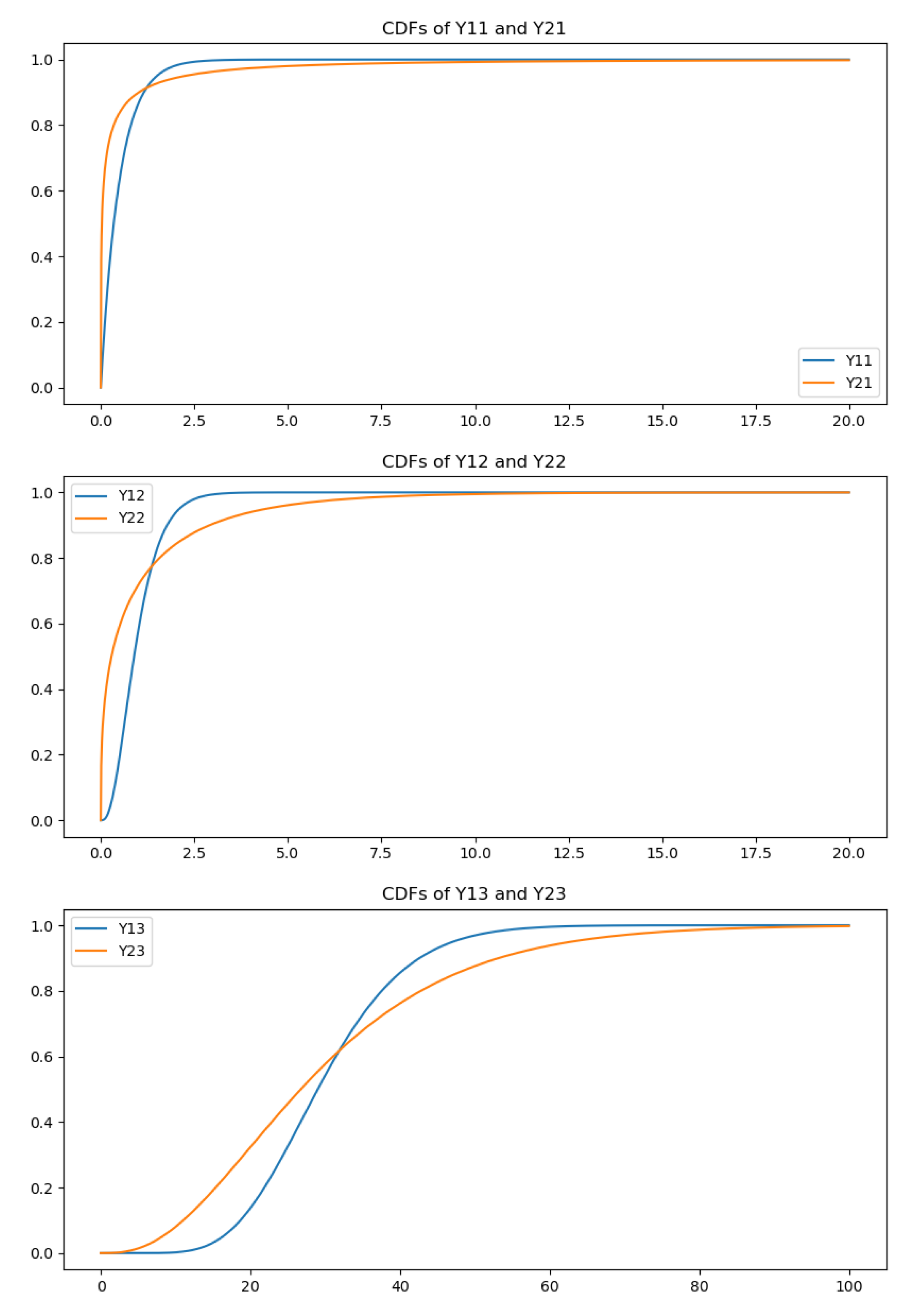
Figure 2.
Comparing the CDF’s of and
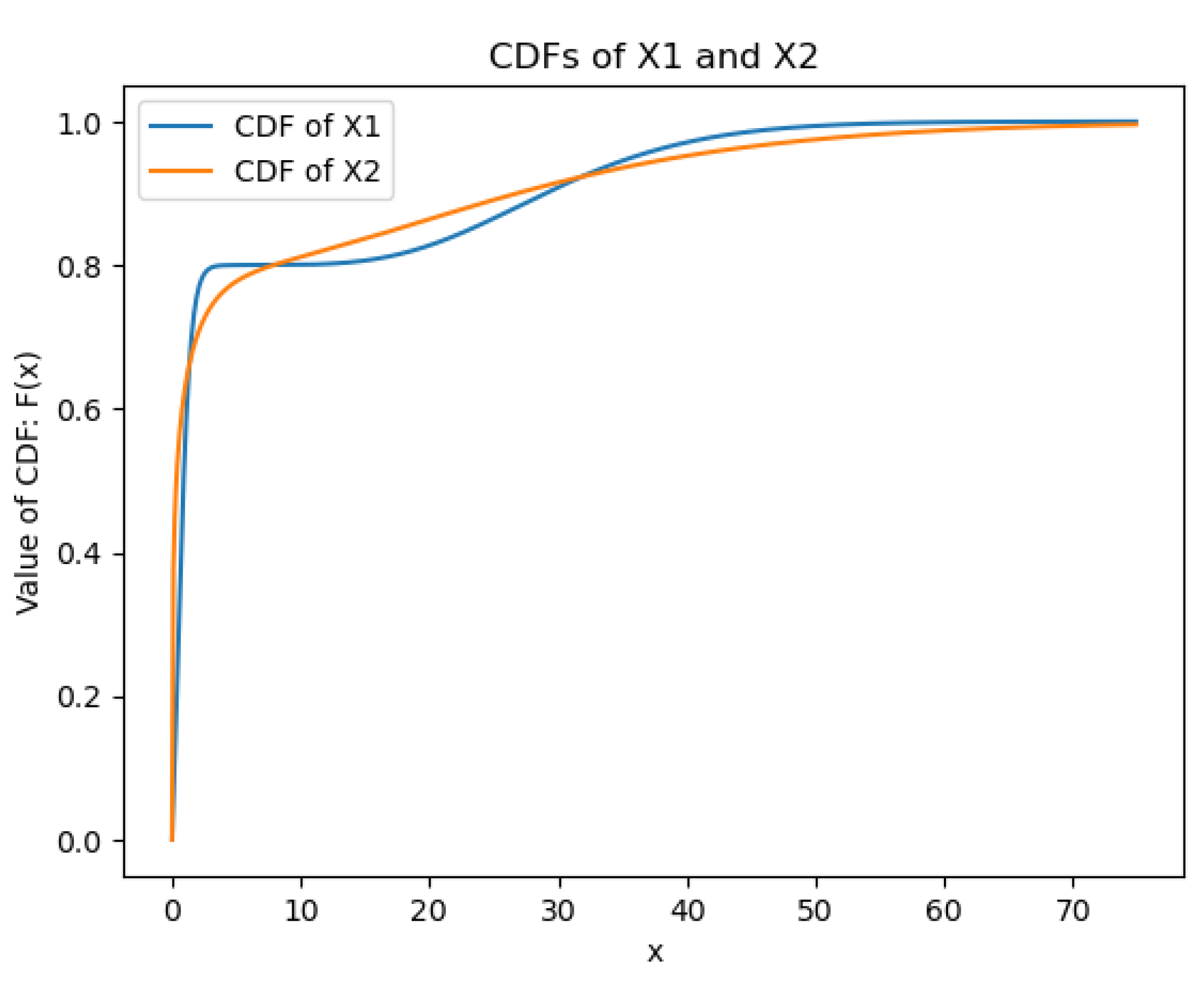
Figure 3.
Comparing the CDF’s of two Dagum densities at T = 1 and 2
Disclaimer/Publisher’s Note: The statements, opinions and data contained in all publications are solely those of the individual author(s) and contributor(s) and not of MDPI and/or the editor(s). MDPI and/or the editor(s) disclaim responsibility for any injury to people or property resulting from any ideas, methods, instructions or products referred to in the content. |
© 2025 by the authors. Licensee MDPI, Basel, Switzerland. This article is an open access article distributed under the terms and conditions of the Creative Commons Attribution (CC BY) license (http://creativecommons.org/licenses/by/4.0/).
Copyright: This open access article is published under a Creative Commons CC BY 4.0 license, which permit the free download, distribution, and reuse, provided that the author and preprint are cited in any reuse.


