
Submitted:
27 August 2024
Posted:
20 September 2024
Read the latest preprint version here
Abstract
Valles Marineris (VM), the most prominent example of a Martian Valley Network, has been extensively studied for over 50 years, yet no detailed examination of the principal azimuths of the system exists. To address this, two methods are presented to precisely calculate the principal azimuths, a Bezier Spline analysis, and a GIS technique. The medial axis of the main canyon of VM was determined analytically from cubic polynomial splines fitted to 93 coordinate points along both north and south edges of the canyon. These splines were optimized, and medial axis points were calculated through numerical techniques that ensured orthogonality between the tangents of each spline and their connecting normal lines. 1,000 Medial Axis points were extracted, and various regression models constructed, including fitting to sinusoidal and cubic polynomial curves, achieving accuracies with R² values of 0.98 and 0.99, respectively. Principal azimuths were obtained using the sinusoidal equation with the slope of the tangent at any point x simply determined by the derivative of the curve’s equation. This analytic approach was cross-validated by a GIS method (using QGIS software), where a vector medial axis was obtained which produced principal azimuths that agreed with values from the analytic study with a correlation coefficient of 1.00, and a p value of 6.43e-65. The findings suggest that a deterministic process plays a significant role in the structural geometry of VM, highlighting its potential importance in the canyon’s formation.
Keywords:
valles marineris
; cubic polynomial splines
; multidimensional optimization
; medial axis
; valley network
; mars
; principal azimuths
; GIS
Bezier Splines
1.1. Introduction
There is conjecture regarding the influence of water in shaping Valles Marineris (VM), the most prominent example of a Martian Valley Network, and interpreted as good evidence of prolonged surface water on Mars (Klokočník et al. 2023, Hynek et al. 2010, Hansjoerg et al. 2018), although the dominant hypothesis attributes the formation of VM to tectonic or erosional forces, subsidence, trough collapse, or a combination (Brustel et al. 2017, Fueten et al. 2017, Andrews-Hanna 2012).
However, despite extensive investigations over 50 years, a conspicuous gap in the literature remains concerning the principal azimuths of the VM system, which are crucial for understanding the directional forces that have shaped the region. An extensive literature search indicates that previous research has focused primarily on determining azimuths between individual features within the VM system, usually within localized canyon areas, and has not addressed the determination of principal azimuths.
This study aims to fill this gap by using a Medial Axis Bezier Spline analysis, a method commonly employed in geomorphological modeling for delineating central trajectories, and cross-validating this approach with a more conventional, algorithmic geographic information system (GIS) technique to determine the principal azimuths of the main canyon. These two analysis methods are rigorously compared to provide statistical evidence confirming the accuracy and reliability of the derived medial axis and azimuthal orientations.
1.2. Main Canyon Definition & CRS
The VM canyon system has distinct morphological complexity because multiple subsidiary canyons, which are ancillary to the main canyon, run parallel or subparallel to it and contribute significantly to the overall topology of the system. In this study, the term ‘main canyon’ is defined as the most pronounced geomorphological feature, trending west to east from Noctis Labyrinth in the west from c15,900 km longitude to Eos Chaos in the east at c18,700 km (see Figure 2).
While the main canyon’s medial axis, as discussed in this paper, is not the midline of the collective features for the entire VM system, establishing the axial symmetry of the main canyon necessarily preserves congruent symmetry in any parallel or subparallel subsidiary canyon.
Reference images were obtained from the THEMIS daytime IR mosaic (100 m/pixel) and JMARS, with an analytical GIS primarily via ArcMapTM. Equidistant Cylindrical Projection was used to preserve accurate distances along meridians via a CRS base: ESRI:103885 (Mars Equidistant 2000 Sphere). Accurate ellipsoid parameters were added with custom code: semimajor axis: 3396.2, semiminor axis: 3376.2
Figure 1.
Shaded area represents the main canyon of the VM. The North and South Canyon edges are labeled and marked by white lines. Melas Chasma is at the midpoint of the main canyon. The approximate starting point of the main canyon is at 15,900 km in the west, terminating at approximately 18,700 km in the east.
Figure 1.
Shaded area represents the main canyon of the VM. The North and South Canyon edges are labeled and marked by white lines. Melas Chasma is at the midpoint of the main canyon. The approximate starting point of the main canyon is at 15,900 km in the west, terminating at approximately 18,700 km in the east.
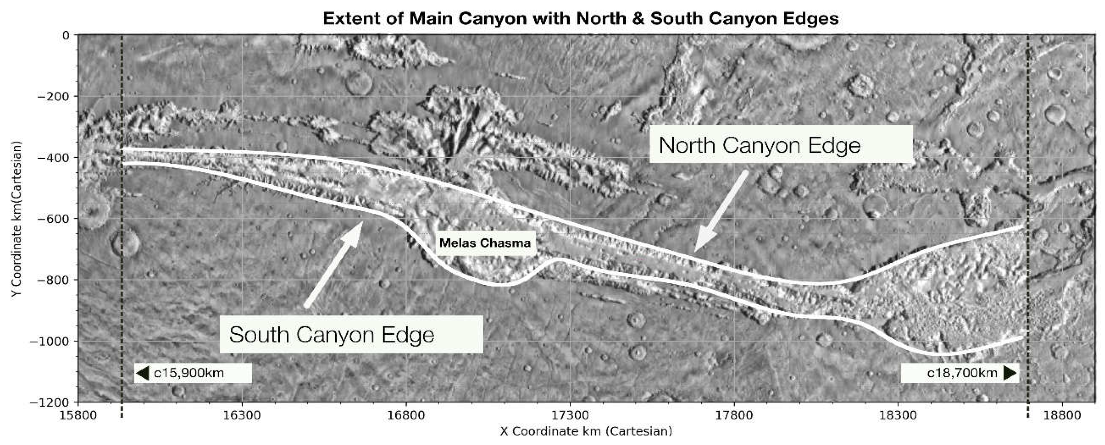
Figure 2.
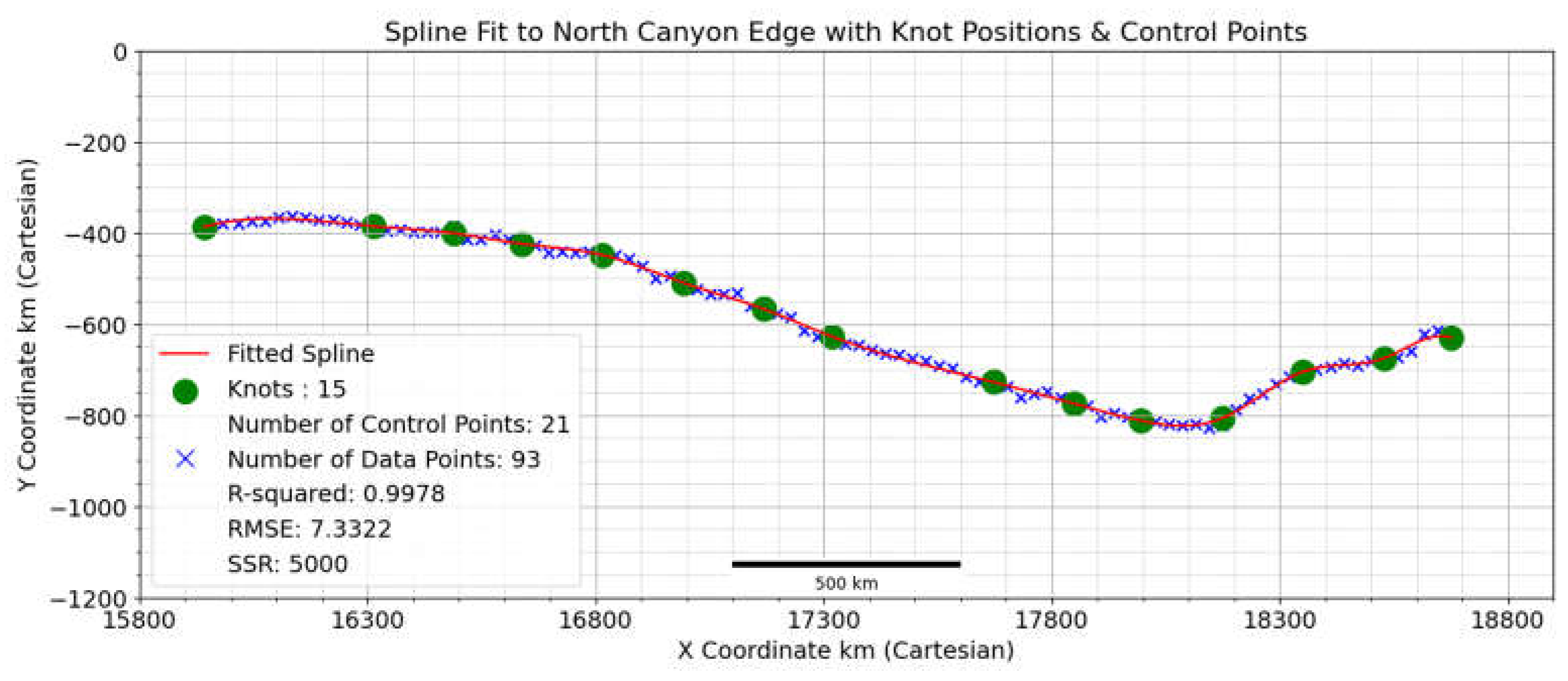
Spline fitted to the North Canyon edge showing 93 coordinate positions and no Knot positions. The smoothing factor used was 5,000, resulting in an SSR of 5,000.
Figure 2.
Spline fitted to the North Canyon edge showing 93 coordinate positions and no Knot positions. The smoothing factor used was 5,000, resulting in an SSR of 5,000.
1.3. Defining Edge Splines
Various methods exist to determine the medial axis of an object, such as Voronoi skeletons, distance transform methods and thinning algorithms such as wave propagation via grassfire algorithms. In this study, a Bezier curve approximation technique was used where univariate spline curves (Dierckx 1981, 1993) were fitted to the North and South Canyon edges of VMs via the UnivariateSpline function from Python’s SciPy library (10).
A total of 93 coordinate points were identified on both North and South Canyon edges, with all points evenly spaced and with longitudinal distances preserved within the Cartesian kilometer-based CRS (ESRI:103885).
The edge splines of the main canyon were constructed with parametric cubic spline continuous functions, ensuring first and second derivative continuity and avoiding sharp changes in the curve’s slope or curvature, which are common in lower-degree splines.
Denoting the splines for the North and South edges as N(t) and S(t), where t is the parameter along the spline or arc length, the spline functions for each Canyon edge in a 2D plane can be written as:

 where:
- Bi,3 (t) and Bj,3 (t) are the cubic B-spline basis functions and are defined over a knot vector that is locally supported
- n and m are the numbers of control points for the North and South edge splines, respectively, determined through the spline fitting process.
- The interval [a, b] represents the domain of the parameter t.
- P1i and P2j are the control points for the North and South edge splines and define the initial shape and direction of the spline, which is then adjusted via the optimization process (see below). While control points do not generally lie on the curve, they act as weights in the combination of basis functions that define the curve.
1.4. Spline Optimization
Univariate spline interpolation involves a piecewise-defined cubic polynomial function that fits a set of data points in a single variable, with knots segmenting the dataset and individual polynomial functions fitted within each segment. The placement of knots and the overall smoothness of the curve in the UnivariateSpline algorithm are regulated by a key parameter: the smoothing factor (s).
When s is unspecified, UnivariateSpline defaults to place knots at every data point, effectively interpolating the data. However, specifying a value for s balances the spline’s smoothness with its adherence to the data by a least-squares optimization process, where the spline coefficients are calculated to minimize the sum of squared residuals between the fitted spline and the data points, subject to the smoothness constraint imposed by s.
Given a set of data points (xi, yi), where i = 1,2,…,N, and a spline function S(x), the goal is to find the spline that minimizes the following objective function:

where:
- The sum of the squared residuals, representing the fit of the spline S(x) to the data points (xi, yi), (lower values indicate a better fit), is added to the integral of the square of the second derivative of the spline, which acts as a measure of the spline’s smoothness. A smoother curve will have a lower value of this integral.
- λ represents the smoothing factor s in UnivariateSpline and is a parameter that balances the two objectives: smoothness of the spline and proximity to the data points.
This optimization problem is solved in UnivariateSpline via numerical methods, as curve fitting problems typically lack closed-form solutions.
With the user-defined s value constraint, the algorithm iteratively adjusts the knots’ positions and the coefficients of the spline to minimize J, capturing the essential trends of the coordinate data while mitigating overfitting.
1.5. Canyon Edge Spline Analysis
The sum of the squared residuals (SSR) shown in the legend of Figure 3 and Figure 4 above, although conceptually distinct, has an important relationship with the smoothing factor s in the UnivariateSpline algorithm, which explains the high SSR value shown.
The smoothing factor serves as an upper bound for the SSR, guiding the algorithm to adjust the spline’s smoothness such that the SSR approaches but does not exceed s. Consequently, the final SSR of a spline often equals the value set for s. Canyon edges, which span >3,000 km, exhibit significant variability due to landslide extensions, erosion and subsidiary canyon intrusion, leading to potentially large residuals, cumulatively resulting in a higher SSR.
A higher smoothing factor is therefore required for the Canyon edge data, enabling the spline to adequately curve to the coordinate data’s underlying trends and allowing for this higher SSR without being excessively constrained by variability.
SSR is a measure of the total deviation of the response values from the fit to the response values, and while a lower SSR may indicate a better fit, it is not a guide to how good the fit is relative to the spread and variability of the data, whereas the R2 value, the coefficient of determination, indicates how well the independent variable explains the variability of the dependent variable by calculating the ratio of SSR to SST (total sum of squares) – R2=1−SSR/SST1.
Both edge splines, which are based on a smoothing factor of 5,000 (SSR 5,000), returned R2 values close to 1, implying that a significant proportion of the total variation in the data is captured and explained by the spline models with minimal deviation from the actual data points. The RMSE (root mean square error) for the charts shown was 7.33, which, in the context of the Canyon edge data measured in kilometers, represents 7.33 km—a mean error equivalent of <0.24%, which is low when contrasted against the vast overall length of the Canyon edges (>3,000 km). To assess how different values of the smoothing factor affect the fit, numbers of knots and control points, several iterations were carried out for each Canyon edge, as shown in Table 1 and Table 2 below:
1.6. Medial Axis Extraction
The medial axis spline is a path equidistant from two edge splines at any point along its length. If the medial axis spline is denoted by M(t), a point M(ti)=(xm(t), ym(t)) on this spline should satisfy the following condition where the distance from any point on the medial axis spline to the nearest point on each edge spline is equal:

Finding midpoints between two splines by simply averaging the distance on a vertical bisector so that Midy =(Northy + Southy)/2, in the context of VM, is not an optimal method for finding the medial points. The VM system trends ≈20° from northwest to southeast, curving in multiple ways; therefore, line segments joining the Canyon edge splines require orthogonality to fully capture the curvature and direction of the splines.
The goal is to find an equal number of points along each of the Canyon edge splines where lines joining pairs of points are perpendicular (normal) to both splines at their respective points of tangency and then find the midpoints M(ti) of these lines. This multidimensional optimization problem has a 2D parameter space that is required to optimize two variables (tnorth) and (tsouth), which are parameters along North and South splines at intersection points with a line segment between both splines (11). The optimization sequence can be written as:
- Smoothing: Apply s = 5000 to both North and South splines.
- Point Pair Identification: Generate a sequence of point pairs {N(ti, S(ti)} for i=1,2,…,n along the entire length of the North and South splines.
- Slope threshold: Calculate the slope at each point on the southern spline as the first derivative of the spline at each point, denoted as Slope_S(ti). Define a threshold value for the slope as slope_threshold
- Conditional processing: For each point pair {N(ti, S(ti)}, check the slope at S(ti):
-
If:Slope_S(ti)< slope_threshold, proceed with subsequent steps (5--10).
-
Else:Skip to the next point pair {N(ti, S(ti)} and proceed with subsequent steps (5 to 10)
- 2.
- Vector: Define L as the vector connecting a point on the North spline at (tnorth) to a corresponding point on the South spline at (tsouth) expressed as L= S(tsouth)−N(tnorth).
- 3.
- Tangent Vectors: Calculate the tangent vectors at tnorth and tsouth as TN (tnorth) and TS (tsouth), respectively.
- 4.
- The perpendicularity function f (tnorth, tsouth) is:f(tnorth, tsouth) = [L · TN(tnorth)]2 + L · TN(tsouth)]2
This function quantifies the squared sum of the dot products of the vector L with the vectors at TN (tnorth) and TS (tsouth).
- 5.
- Multidimensional Optimization: adjust tnorth and tsouth to minimize f (tnorth, tsouth) to zero and therefore the perpendicularity of L with both TN (tnorth) and TS (tsouth).
- 6.
- Midpoint Calculation: Use the perpendicular bisector to calculate the midpoint M(ti) of L, which represents the optimized medial axis point for each ti
- 7.
- Iteration: Repeat the process for 1,000 points to compile the set {M(ti)}.
(This sequence forms the basis of the logic to produce Python code, which, in this study, was written to determine the Medial Axis with the SciPy-optimizefunction from Python’s SciPy library (11)).
Normal line equivalence at points (tnorth)and(tsouth) requires the tangents of the curve at each point to be parallel. For the original dataset of the Canyon edge coordinate points, this condition is potentially difficult to meet, as there may be significant direction changes in the Canyon edges.
However, the smoothing factor used in the first step of the above procedure helps to regularize the data by reducing noise and minor fluctuations and facilitates the multidimensional optimization process by making the behavior of the spline (especially its tangents) more consistent and less prone to abrupt changes. Too much variability in the coordinate data might otherwise mislead an optimization algorithm to either prevent convergence or alternatively produce a local solution that is not globally optimal. For consistency in this study, a smoothing factor of 5,000 was used for both the North and South splines.
A specific conditionality function is also integrated into the above sequence (steps 3 & 4) to address the anomaly at the midpoint of the South Spline, where the region of Melas Chasma imposes pronounced southward semicircular extrusions along the Canyon edge and spline representation (see Figure 2). The steeper tangent slopes in this region potentially lead to complexities in the algorithm’s ability to resolve accurately.
To avoid this, the algorithm employs a threshold-based decision process where if the calculated slope at any given point exceeds a predetermined angle – set for this study at ±25 degrees – the algorithm omits processing for that particular point pair, advancing instead to the subsequent pair. Given the localized nature of the Melas Chasma steep tangent slopes, this adjustment impacts only a negligible portion of the overall spline representation.
The determination of each coordinate point M(ti) in the saved array {M(ti)} can be described more formally by optimizing the objective function J1, which enforces equidistance and orthogonality constraints for points on the medial axis spline:

where:
- d1(ti) and d2(ti) are the distances from M(ti) to N(ti) and S(ti), respectively.
- O1(ti) and O2(ti) are measures of the deviation from orthogonality at M(ti) to N(ti) and S(ti), respectively. This is computed as the sum of the squares of the dot product of the vector L with the tangent vectors TN and TS.
- λ1 and λ2 are weighting parameters for the importance of equidistance and orthogonality in the objective function.
- ti represents the parameter values at which the spline and constraints are evaluated.
- N is the number of points along the spline where calculations are made.
The array of medial axis coordinate points {M(ti)} was used to construct a medial axis spline in a 2D plane via the same method as the Canyon edge splines were created via the UnivariateSpline algorithm, formally expressed as:

where:
- M(t) represents the medial axis spline.
- Bk,3(t) are the cubic B-spline basis functions for the medial axis spline.
- Pmk are the control points of the medial axis spline.
- p is the number of control points for the medial axis spline, which is determined through the spline fitting process.
- The interval [c, d] represents the domain of the parameter t for the medial axis spline.
For the medial axis spline optimization:
 where:
- (xi, yi) are the coordinate points that the medial axis spline is intended to fit.
- q is the number of data points.
- The sum of the squared residuals, representing the fit of the medial axis spline to the data points (xi, yi), is added to ∫ [M’′(x)]2dx, the integral of the square of the second derivative of the spline, and acts as a measure of the spline’s smoothness.
- λ is the smoothing parameter that balances the trade-off between the fit to the data points and the smoothness of the spline (represented by the smoothing factor s in UnivariateSpline).
As was the case for constructing the Canyon edge splines, this objective function JM balances the dual goals of fitting the medial axis spline closely to the determined medial axis points while also maintaining a smooth curve controlled by the choice of the smoothing parameter.
1.7. Medial Axis Spline Charts
Figure 5.
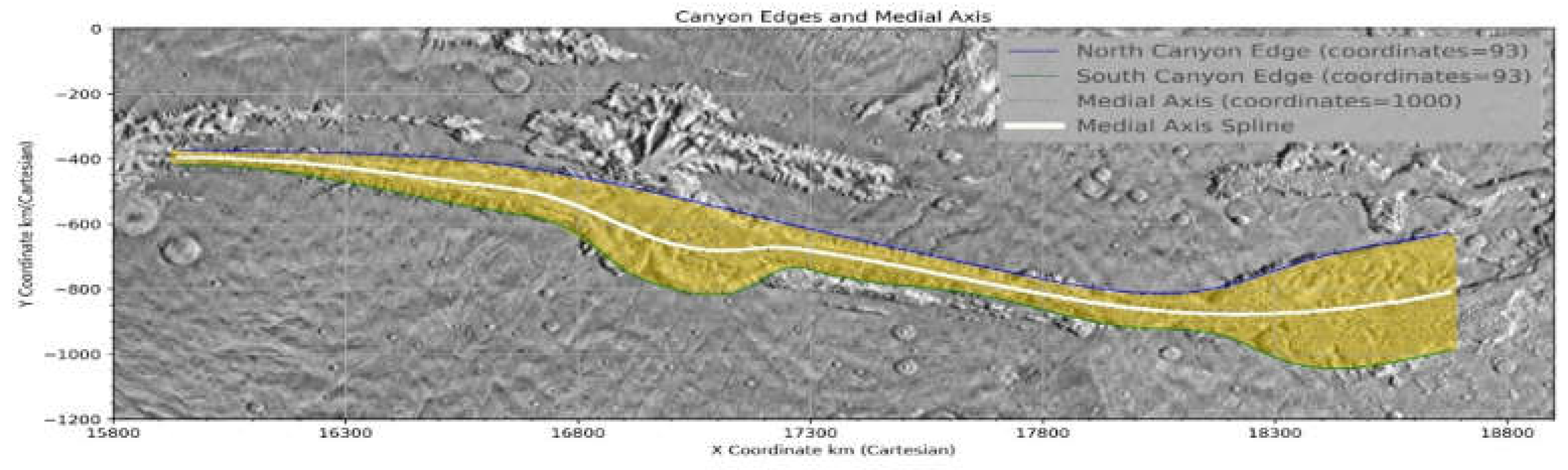
Positions relative to a THEMIS daytime IR mosaic composite image of Valles Marineris of the fitted splines (North, South & Medial). The shaded area represents the extent of the VM Main Canyon.
Figure 5.
Positions relative to a THEMIS daytime IR mosaic composite image of Valles Marineris of the fitted splines (North, South & Medial). The shaded area represents the extent of the VM Main Canyon.
Regression Analysis
2.1. Model: Sinusoidal
Various curve fitting models were considered for fitting to the median axis coordinate data of 1000 points. A visual inspection of the medial axis plot (see Figure 6} suggested a possible sinusoidal fit to the data, and an initial guess for this fit, its determination and comparison to final fit values, is shown in Table 3 below:
To optimize the sinusoidal model parameters, the iterative least-squares Levenberg–Marquardt method was used, implemented via SciPy’s ‘optimize’ and ‘curve_fit’ functions. This method minimizes the residual sum of squares, a common objective function (loss function) in regression analysis. The initial parameter estimates, shown in Table 5, resulted in reliable model convergence, with final values closely matching the initial guess. For comparative analysis, linear, geodesic path, and cubic polynomial models were included, as shown in both Table 4 and Figure 7. The fitted sinusoidal curve was determined as:

2.2. Model: Cubic Polynomial
Cubic polynomial models are widely used in situations where a balance is needed between model complexity and the ability to accurately represent the underlying trends of the data without the risk of overfitting associated with higher degree models. The loss function for n data points can be defined as:

This loss function was minimized by a least squares algorithm implemented in Python by scipy.optimize.curve, and the fitted cubic polynomial was determined for 1000 coordinate points as:

2.3. Model: Linear
In the literature, VM is typically described as exhibiting linear characteristics or even, more casually, as being a linear feature. To critically evaluate this assertion, a linear model was included as a reference or baseline in this analysis. This approach allows for a direct comparison with other models to demonstrate that a more complex model structure than that which is purely linear better represents the underlying data patterns.
2.4. Model: Geodesic
A geodesic model was chosen to evaluate any significant divergence from the geodesic trajectory by the medial axis, which would indicate influences or additional factors beyond simple distance minimization. Substantial deviations from the geodesic require a causal explanation, whether stochastic, deterministic or a combination (e.g., tectonic split in the crust, water/lava erosion, or other causal factors).
The ‘Geod’ object from the ‘pyproj’ library, which is optimized for handling latitude and longitude data for distance and angle calculations on a spherical model (Mars), was used to define the geodesic path. The longitude values were normalized to the 0--360° range in a standard positive east longitudinal system, and paths were optimized to prevent wrapping around the sphere. The start and end coordinates were set at -6.9° latitude, 270° longitude, and -13.8° latitude, 316° longitude, respectively.
Based on Mars’s mean radius of 3396.2 kms, the ‘Geod’ object generated 100 intermediate coordinate points along the calculated great circle route. For quantitative analysis and plotting in linear units, a conversion from latitude and longitude to kilometers was conducted via a ‘numpy’ function applying the Equidistant Cylindrical projection (ESRI:103885). The latitude and longitude were adjusted relative to a central point (defaulted to 0°) and then converted to radians multiplied by the mean radius of Mars to compute the Cartesian coordinates, where xrepresents the horizontal distance and y represents the vertical distance from the central point in a planar projection of Mars. The geodesic path, converted from original latitude/longitude coordinates to Cartesian coordinates, was modeled via a quadratic polynomial to accommodate the expected slight curvature. The best-fit polynomial, determined through least squares fitting, is given by the following equation:

2.5. Model Comparison - 100 Coordinate Points
The plot shown in Chart 7 is not at a sufficient scale to distinguish separate sinusoidal and cubic polynomial fitted curves —there is considerable overlap. However, a clearer way of discriminating between each model can be seen in Table 4, where a dataset of 100 Medial Axis points was examined according to a variety of standard metrics. The Cubic polynomial model’s ability to adapt to more complex patterns, although numerically showing the best performance, does not provide a significant advantage, suggesting that the complexity it adds may not be necessary to capture the primary dynamics of the data, thereby tending to validate the simpler sinusoidal model.
Cubic polynomial models have more coefficients for each degree of the polynomial, allowing a fit that captures more fluctuations in the data than a sinusoidal model, which is characterized by a single frequency, amplitude, and phase. The Akaike information criterion (AIC) and the Bayesian information criterion (BIC) are standard techniques for comparing models with different complexities, with the AIC penalizing complexity by adding twice the number of parameters (2k) and the BIC further multiplying the number of parameters by the logarithm of the data points (log(n) *k). However, in both cases, while complexity is penalized, a good fit is always rewarded, and if the polynomial model’s complexity leads to a better fit, this can suggest improved performance despite a greater number of parameters.
2.6. Kernel Density Estimate for Residuals
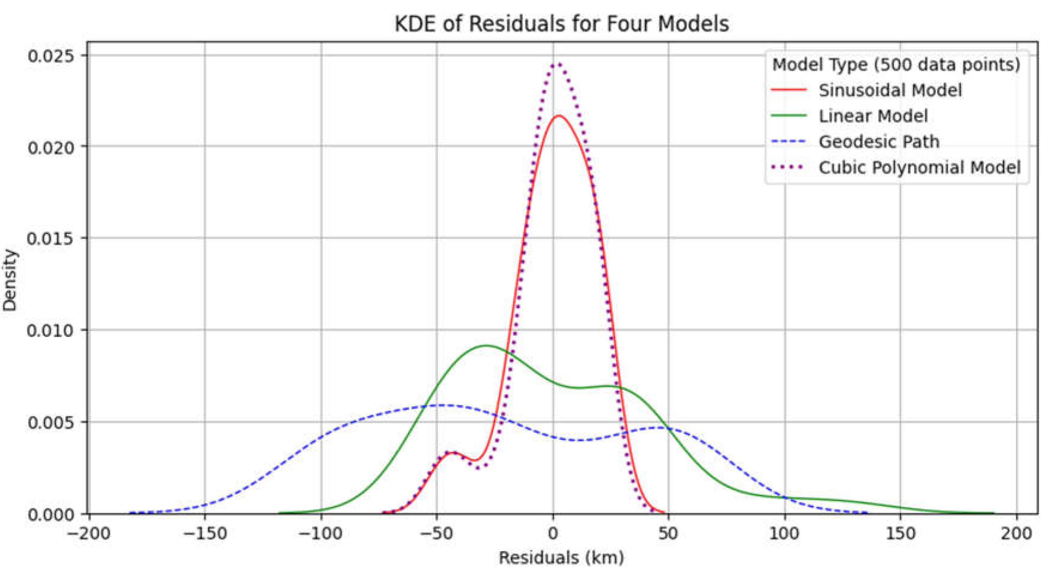
A kernel density estimation plot of all four models also reveals a close match for both sinusoidal and cubic polynomial models, with a unimodal distribution of sharp high central peaks for both indicating a high concentration of residuals near zero and therefore a good fit with minimal error. The other two comparative models, linear and geodesic path, display pronounced bimodal distributions, suggesting that both have two distinct residual groups where the models are underfitting or overfitting and cannot capture the curvature or pattern in the data.
Figure 8.
KDE of the residuals for the four models.
2.7. Data Scaling
To evaluate model robustness and efficiency across a spectrum of data volumes, an AIC analysis was used based on a range from 25 coordinate points to 1,000 points, which were extracted from the original medial spline calculation curve. The linear trend on chart 9 shows that as the dataset size increases, the complexity of the models scales up linearly, indicating no sudden increase in complexity, which might otherwise imply overfitting or poor scalability.
Figure 9.
Data scaling for 25–1,000 coordinates compared with the AIC value.
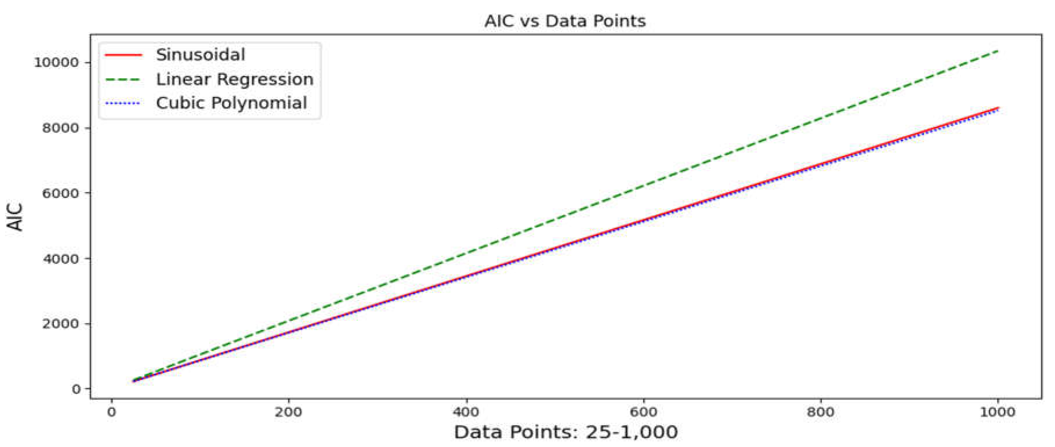
The cubic polynomial model consistently maintains a marginal advantage over the sinusoidal model, yet both overlap substantially at the scale of the chart. Both significantly outperform the linear model used as a reference.
2.8. Azimuths
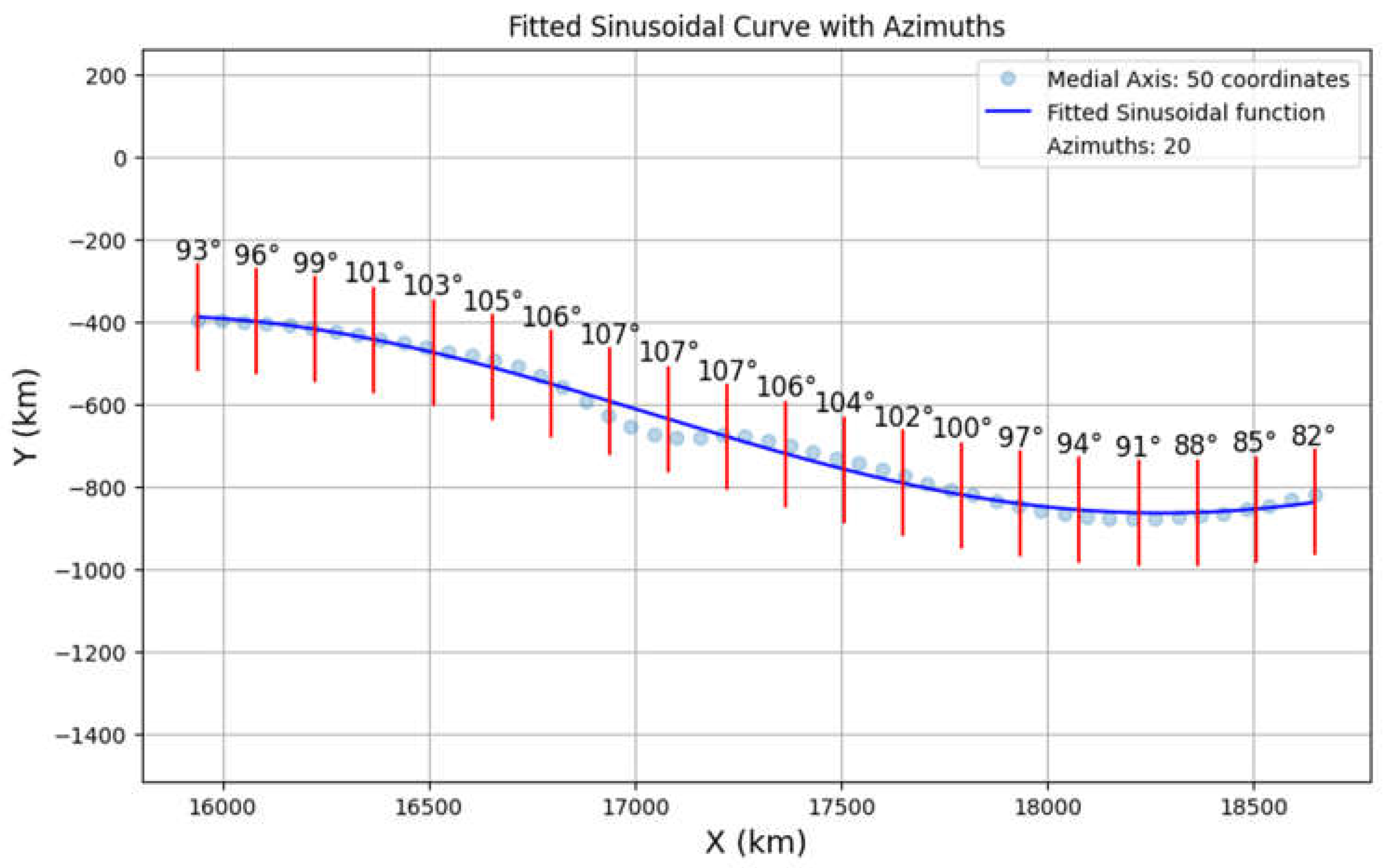
Fitting a sinusoidal (or cubic polynomial) curve to the median axis coordinate data has the significant advantage of providing an efficient and practical method to determine the principal azimuths of the main canyon by easily calculating tangents, with the slope of the tangent at any point x simply determined by the derivative of the curve’s equation. Using this method, potentially unlimited datasets of azimuths can be generated for the curve; however, only 20 azimuths were generated for display clarity on a chart (see Figure 10). A total of 1,000 medial axis coordinates were curve fitted to a sinusoidal function to derive the best fit equation:

Figure 10.
Extraction of 20 azimuth values in a Cartesian CRS.
Using standard differentiation techniques (product rule and chain rule), the derivative of the sinusoidal function, which represents the slope at any point x, is found to be:

Assuming an initial position (x0, y0), the calculated slope of the tangent is converted to an angle via the arctangent function, which yields an angle θ in radians from the positive x-axis:

To convert this Cartesian angle into an azimuth (north-based bearing), the coordinate system is rotated by 90° - θ0, and to ensure that all azimuths are positive and appropriately normalized, the azimuth is adjusted via the modulo operation: azimuth = (azimuth + 360) mod 360. For the iteration of azimuths, the change in azimuth over distance △x uses the derivative:
 with the next azimuth value predicted by:
 and to ensure that θ n+1 is positive:
 where:
- x: Independent variable representing the horizontal coordinate.
- y(x): The sinusoidal function describing the vertical coordinate as a function of x.
- y′(x): The derivative of y(x) represents the slope of the function at any point x.
- θ: The azimuth angle in degrees, measured clockwise from north.
- θ0: The initial azimuth angle at the starting position.
- Δθ: The change in the azimuth angle over a distance Δx
- Δx: A change in the horizontal coordinate x.
3.1. Gis Validation
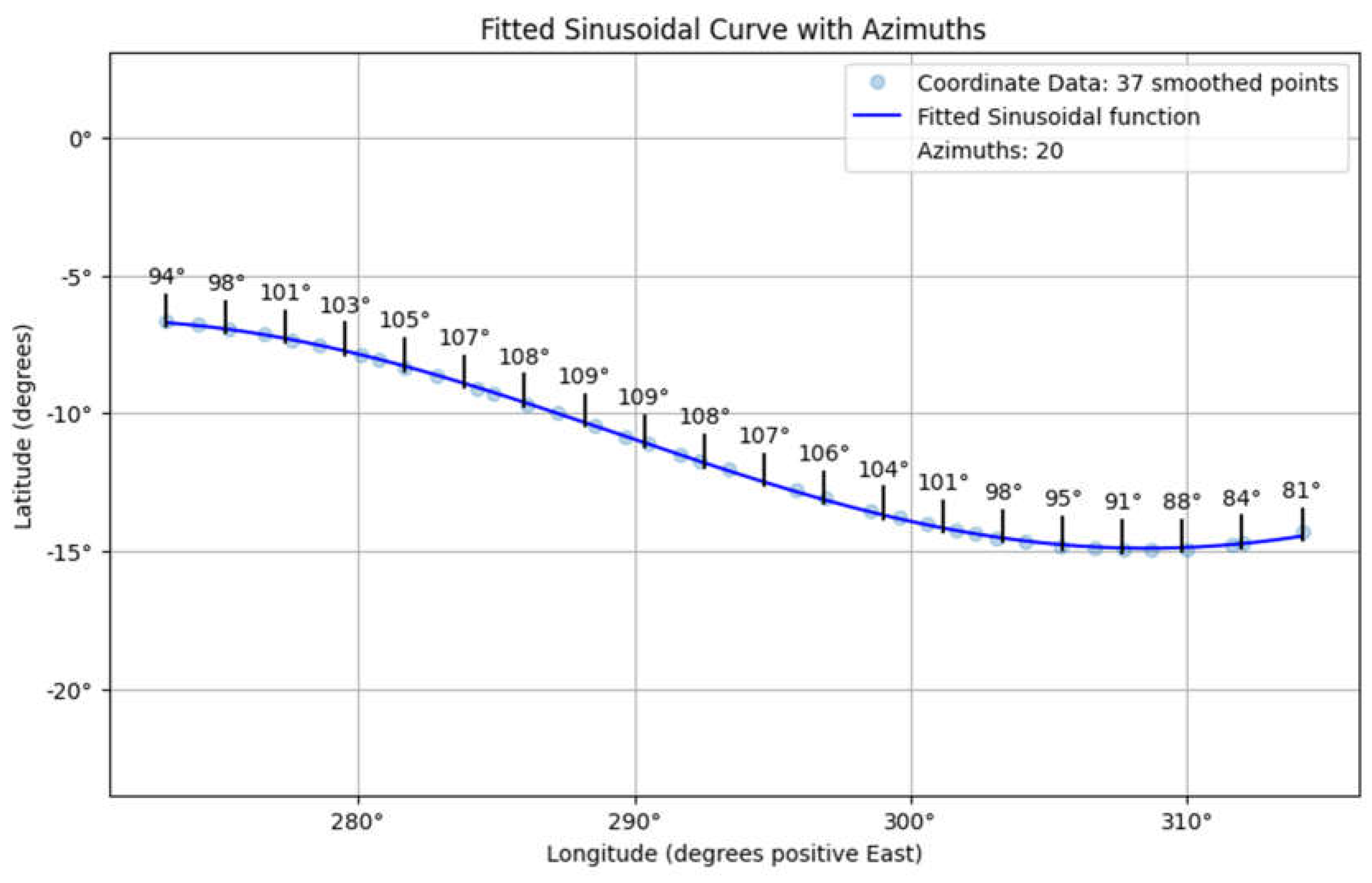
In addition to the above detailed analytic techniques, a computational GIS approach was also undertaken via QGIS software. The aim was to cross-validate the analytic results, particularly the azimuth calculations, with azimuths derived algorithmically and in an alternative CRS geodetic coordinate system. Several tools and plugins were used to automatically detect edges and vectorize. A brief description of the workflow in the QGIS is as follows:
- High-resolution DEM data (JMARS) and Georeference were acquired with CRS ESRI:107971 (Mars 2000 Sphere).
- Geotrace North and South Canyon edges of the main canyon with an edge detection algorithm and appropriate threshold values (canny edge detection)
- Buffer each raster Canyon edge, merge raster layers to vectors, extract vertices, and then process with the Voronoi polygon tool.
- From the vectorized Voronoi skeleton extract the medial axis line
- Segment medial axis vector via a field calculator and derive azimuths for each segment
Figure 11.
Extraction of 20 azimuth values in a Geodetic CRS. Medial axis spline smoothed with an SSR of 5,000.
Figure 11.
Extraction of 20 azimuth values in a Geodetic CRS. Medial axis spline smoothed with an SSR of 5,000.
3.2. Gis/Analytic Comparison
Two sets of azimuths, one from the analytic approach (Cartesian) and one from the GIS methodology (Geodetic), were compared to assess the accuracy and correlation of both methods. 50 azimuths were extracted for each set (see
Table 5).
The azimuths derived independently from the geodetic and Cartesian CRS exhibit a high degree of similarity; however, a slight difference in the mean azimuths was observed (Geodetic: 100.25 degrees, Cartesian: 99.07 degrees). This variation can be attributed to several factors inherent to the different methods employed. Aside from potential CRS projection transformation discrepancies (which can introduce minor errors due to the approximations used in the conversion processes), the principal way discrepancies are likely to have occurred is with the collection of data for each set.
The geodetic azimuths were calculated algorithmically via the GIS program QGIS, whereas the Cartesian azimuths were determined analytically via Bezier splines. Slight discrepancies in the edge detection of canyons and spline derivation from selected coordinate points on canyon edges affect the final azimuth calculations. However, the significant correlation between the two sets of azimuths (correlation coefficient = 1.00, p value = 6.43e-65), despite the methodological differences in obtaining them, indicates strong agreement between the two approaches.
Although the geometric and Cartesian azimuths differ slightly in terms of their exact values, they still follow the same general sinusoidal trend, which is reflected in the high correlation coefficient and demonstrates that the two datasets have a very strong linear relationship, i.e., effective cross-validation. The small difference in means, while statistically significant (paired t test: t statistic = 9.59, p value = 7.94e-13), indicates that even minor differences can be detected with high precision due to the paired nature of the data and the large sample size.
4. Discussion
This study derived the medial axis for the main canyon of the VM via both an analytic approach with Bezier splines and an algorithmic approach with GIS software (QGIS). The results were compared statistically to assess the correlation between the two methods by comparing the azimuths produced by both methods. The statistical analysis revealed a correlation coefficient for both sets of azimuths of 1.00 and a p value of 6.43e-65. This strong correlation validates the accuracy and reliability of both approaches in mapping the medial axis of the VM.
Establishing a primary azimuthal framework for the VM system provides a critical reference or baseline for subsequent azimuth calculations within individual canyons. This framework enhances the accuracy of localized analyses, enabling detailed comparative studies, and supports hierarchical and cross-canyon studies, enabling a multiscale approach.
In the regression analysis, four models were compared: sinusoidal, cubic polynomial, linear, and geodesic. The sinusoidal and cubic polynomial models provided the best fit, demonstrating significant alignment with the derived medial axis at distances greater than 3,500 km. The fit of the sinusoidal and cubic polynomial models over such a large distance is unexpected and suggests that underlying mechanisms influence the formation of the main canyon and its medial axis in a predictable manner.
The challenge lies in understanding which geological processes, such as planetary tectonics or erosion, might create patterns that align so accurately with these mathematical models. An accurate fitted curve model, particularly one that fits well over a large distance, implies a deterministic causation process, as such models typically represent regular, periodic, and predictable phenomena rather than stochastic, unpredictable phenomena. A potential focus for further research is to examine the principal azimuths of the main canyon for their applicability to all features of the VM system by quantifying the exact degree of congruent symmetry or parallelism in all subsidiary canyons or features.
5. Limitations
The selection of coordinate data on the Canyon edges to construct Bezier splines has inherent subjectivity; however, the choice of evenly spaced x-axis coordinates (longitudes) was precisely aimed at minimizing any subjective bias.
Selection effects are also inevitably involved in the choice of where precisely the main canyon of VM originates and ends (see
Figure 2). VM trends west to east, and the first identifiable main canyon edges can be seen in the west, as they emerge from the heavily fractured area of the Noctis Labyrinth at approximately 15,900 km on the x-axis in a Cartesian CRS or 265° east of a positive east reporting system in a Geodetic CRS.
The termination of the main canyon edges is less clear in the east, where large outflow channels from VM have created a poorly defined chaotic terrain at Eos Chasma and Capri Chasma, leading to Aurorae Chaos. This study takes the last well-defined main canyon edge to be at approximately 18,700 km or 320° east, after which the canyon edges become highly irregular. This easternmost point can be seen as the boundary between the main canyon and the beginning of the outflow networks that eventually lead to the northern expanse of Chryse Planitia.
6. Conclusions
This research presents two methodologically robust approaches to calculating the medial axis of the main canyon of Valles Marineris. A Bezier approximation spline technique coupled with multidimensional optimization was compared with an algorithmic GIS approach. Both methods are highly reproducible and yield accurate values for the medial axis coordinates. In addition, both methods are able to determine the principal azimuths of the main canyon of the VM and statistically show a high degree of correlation, therefore effectively cross validating each approach. The fact that a sinusoidal model is an accurate fit to the medial axis is an unexpected result and suggests that deterministic processes were primarily involved in the formation of Valles Marineris.
The data that support the findings of this study are available from the corresponding author, D James, upon request: treleasemill@hotmail.com
References
- Klokočník J, Kletetschka G, Kostelecký J, Bezděk A, 2023. 2023; Gravity aspects for Mars, Icarus, Volume 406, 2023, 115729, ISSN 0019-1035. [CrossRef]
- Hynek, B. M. , Beach, M., Hoke M. R. 2010. Updated global map of Martian valley networks and implications for climate and hydrologic processes. Journal of Geophysical Research: Planets, 115(E9). [CrossRef]
- Hansjoerg, J. Seybold et al. 2018. Branching geometry of valley networks on Mars and Earth and its implications for early Martian climate. Sci. Adv.4, eaar6692. [CrossRef]
- Brustel, C. , Flahaut, J. , Hauber, E., Fueten, F., Quantin, C., Stesky, R. Davies, G. R., 2017. Valles Marineris tectonic and volcanic history inferred from dikes in eastern Coprates Chasma, Journal of Geophysical Research: Planets, 10.1002/2016 JE00 5231, 122, 6, (1353–1371). [Google Scholar]
- Fueten, F. , Novakovic, N., Stesky, R., Flahaut, J., Hauber, E., 2017. The Evolution of Juventae Chasma, Valles Marineris, Mars: Progressive Collapse and Sedimentation. Journal of Geophysical Research. Planets, 122 (11), pp.2223-2249. 〈hal-02130274〉. [CrossRef]
- Andrews-Hanna, J. C. 2012. The formation of Valles Marineris: 1. Tectonic architecture and the relative roles of extension and subsidence. Journal of Geophysical Research: Planets, 117(E3). [CrossRef]
- Dierckx, P. ,1981. An improved algorithm for curve fitting with spline functions, report tw54, Dept. Computer Science, K.U. Leuven.
- Dierckx, P. , 1993. Curve and surface fitting with splines, Monographs on Numerical Analysis, Oxford University Press, 1993.
- scipy.interpolate.UnivariateSpline. SciPy v1.11.4 Manual https://docs.scipy.org/doc/scipy/reference/generated/scipy.interpolate.UnivariateSpline.
- Optimization and root finding. SciPy v1.11.4 Manual https://docs.scipy.org/doc/scipy/reference/optimize.html.
Figure 3.
Spline fitted to the South Canyon edge showing 93 coordinate positions and knot positions. The smoothing factor used was 5,000, resulting in an SSR of 5,000. More knots and control points were used than the North Canyon edge spline, as the South Canyon edge has more variability.
Figure 3.
Spline fitted to the South Canyon edge showing 93 coordinate positions and knot positions. The smoothing factor used was 5,000, resulting in an SSR of 5,000. More knots and control points were used than the North Canyon edge spline, as the South Canyon edge has more variability.
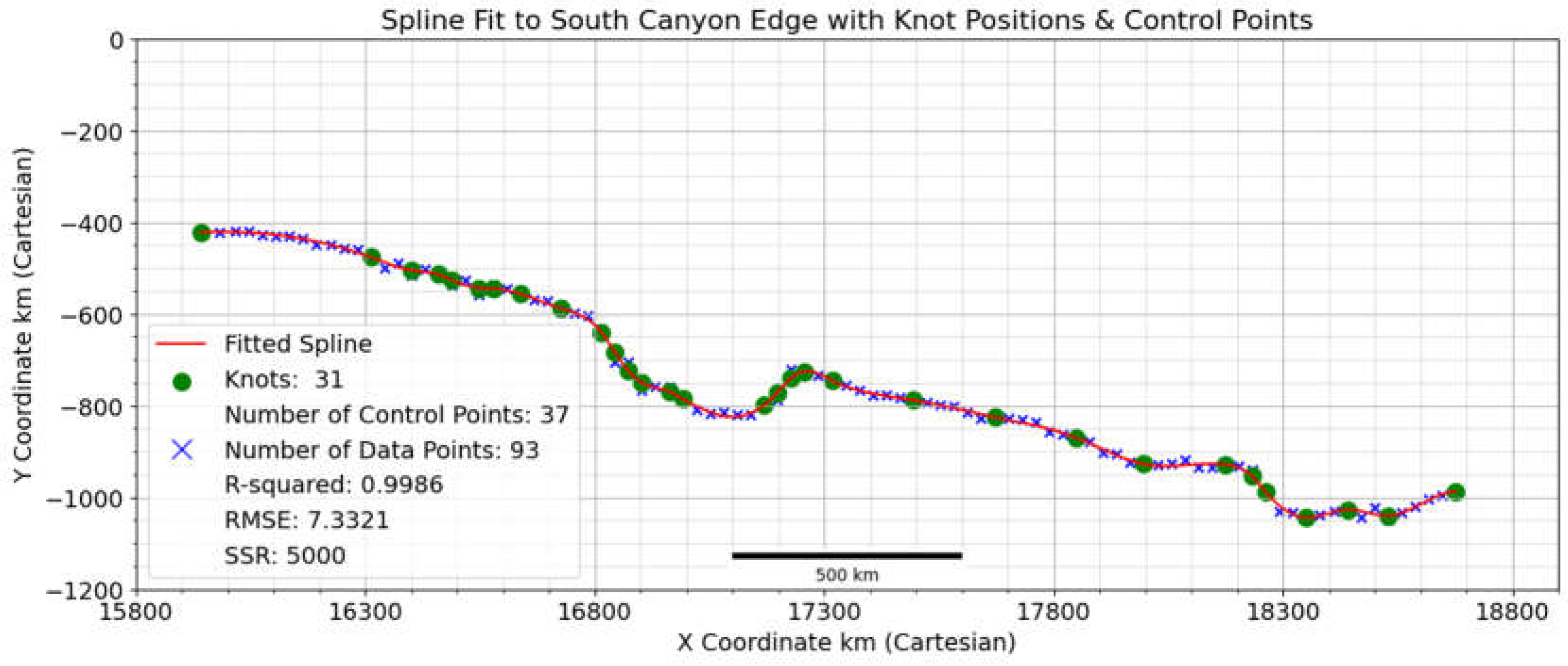
Figure 4.
Medial axis spline fitted to 1,000 median axis points. The smoothing factor used was 5,000, resulting in 12 knots and an SSR of 5,000.
Figure 4.
Medial axis spline fitted to 1,000 median axis points. The smoothing factor used was 5,000, resulting in 12 knots and an SSR of 5,000.
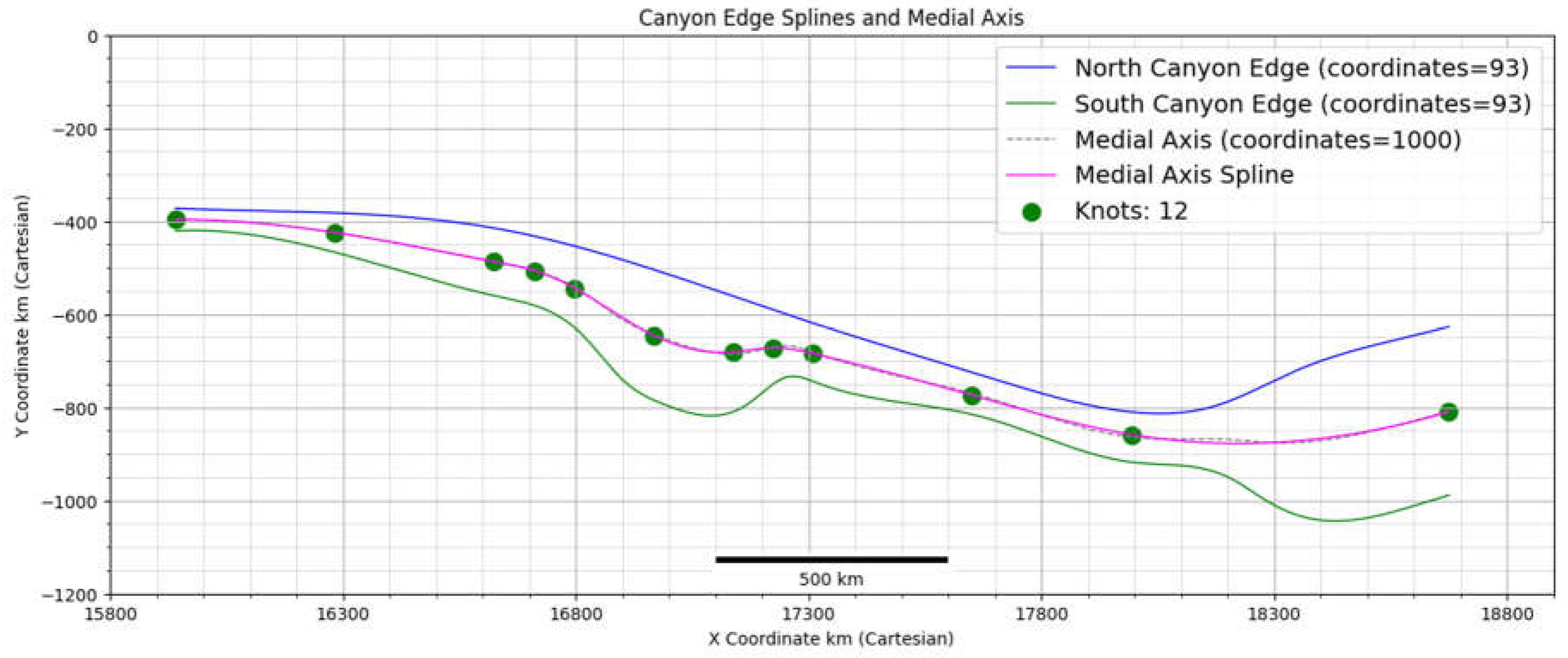
Figure 6.
Chart showing the medial axis spline based on 1,000 medial axis coordinates, without showing Canyon edge splines, for evaluation of potential medial axis symmetries.
Figure 6.
Chart showing the medial axis spline based on 1,000 medial axis coordinates, without showing Canyon edge splines, for evaluation of potential medial axis symmetries.
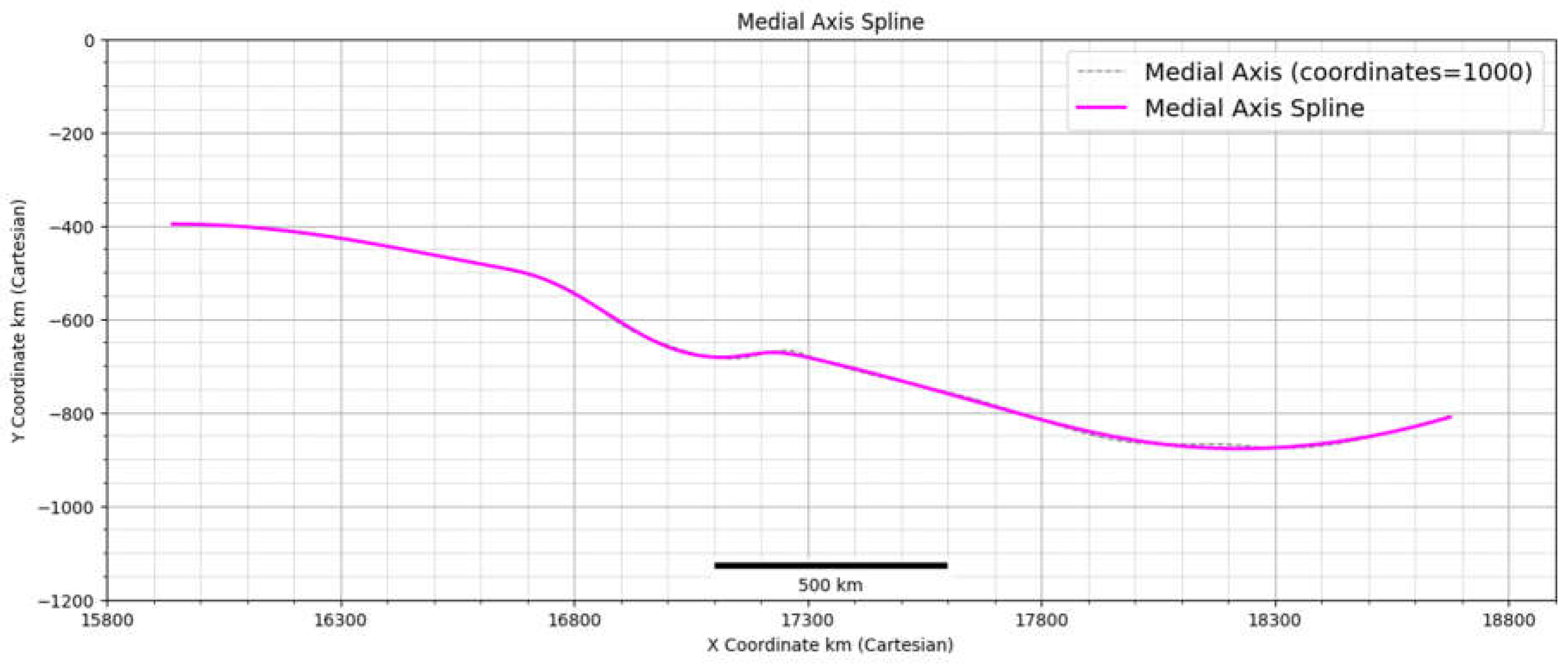
Figure 7.
Chart showing 4 Models fitted to medial axis coordinates (1,000).
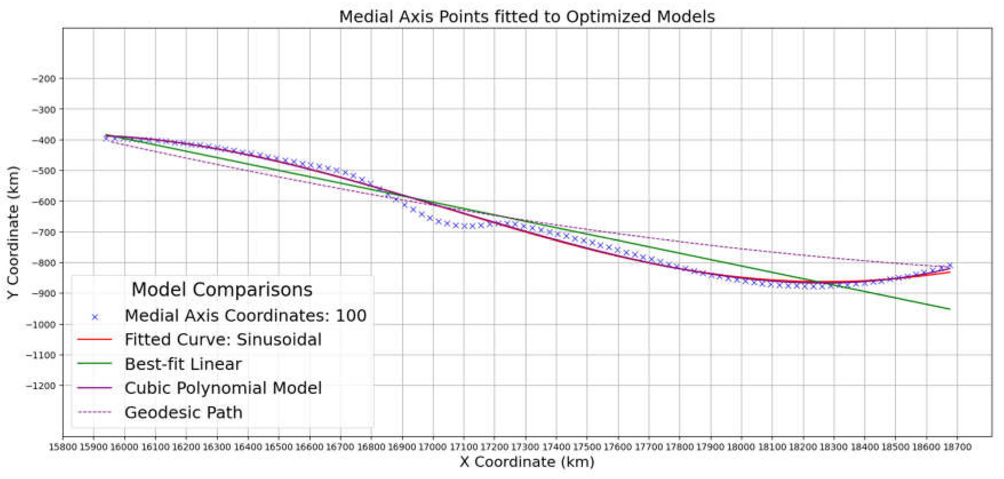

Table 1.
North Canyon Edge.
| North Canyon Edge – Coordinate Points = 93 | ||||
|---|---|---|---|---|
| SSR/smoothing factor | Knots | Control Points | R2 | RMSE |
| 10 | 84 | 89 | 1.0000 | 0.328 |
| 100 | 71 | 78 | 1.0000 | 1.036 |
| 1000 | 40 | 49 | 0.9996 | 3.277 |
| 5000 | 15 | 21 | 0.9978 | 7.332 |
| 10,000 | 8 | 14 | 0.9956 | 10.369 |
Table 2.
South Canyon Edge.
| South Canyon Edge – Coordinate Points = 93 | ||||
|---|---|---|---|---|
| SSR/smoothing factor | Knots | Control Points | R2 | RMSE |
| 10 | 85 | 91 | 1.0000 | 0.3279 |
| 100 | 72 | 79 | 1.0000 | 1.037 |
| 1000 | 47 | 55 | 0.9997 | 3.277 |
| 5000 | 31 | 37 | 0.9986 | 7.332 |
| 10,000 | 15 | 21 | 0.9972 | 10.368 |
1 In UnivariateSpline documentation, the SSR is only required to be ≤s, so for some splines, it can theoretically be less. For all splines detailed in this paper it was equal.
Table 3.
Methodology for Initial Guess (Sinusoidal).
| Initial Guess | Methodology for Initial Guess | Final Fit Values | % Change | |
|---|---|---|---|---|
| Parameter | ||||
| Amplitude (A) | -236 | A ≈ (max(y) - min(y))/2 | -239.01 | -1.27% |
| Angular Frequency (ω) | -0.0018 | ω ≈ 2π * (Cycles/Range of x) | -0.00128 | 28.90% |
| Phase Shift (φ) | 261.02 | Align first peak with model | 251.1 | -3.80% |
| Vertical Shift (B) | -631.57 | B ≈ mean(y) | -624.05 | 1.20% |
Table 4.
Comparison of regression metrics.
| Log-Likelihood | AIC | BIC | SD of Residuals | R² | Adjusted R² | RMSE | |
|---|---|---|---|---|---|---|---|
| Model | |||||||
| Cubic Polynomial Model | -425.196 | 858.392 | 868.812 | 17.082 | 0.99 | 0.99 | 16.996 |
| Sinusoidal Model | -429.416 | 866.832 | 877.253 | 17.818 | 0.989 | 0.989 | 17.729 |
| Linear Regression Model | -519.145 | 1042.29 | 1047.5 | 43.707 | 0.935 | 0.935 | 43.488 |
| Geodesic Path | -552.37 | 1108.74 | 1113.95 | 35.24 | 0.876 | 0.873 | 60.319 |
Table 5.
Mean summary and correlation metrics.
| Mean Summary | |||
|---|---|---|---|
| Metric | Geodetic Azimuths | Cartesian Azimuths | Comparison |
| Mean (degrees) | 100.25° | 99.07° | Geodetic Mean slightly higher |
| Standard Deviation | 7.95° | 7.16° | Similar variability |
| (degrees) | |||
| Correlation Metrics | |||
| Metric | Value | Interpretation | |
| Correlation Coefficient (r) | 1 | Perfect Linear relationship | |
| p value (Correlation) | 6.45e-65 | Highly significant correlation | |
| Paired t test (t-statistic) | 9.59 | Significant difference in means | |
| Paired t test (p value) | 7.94e-13 | Highly significant difference | |
Disclaimer/Publisher’s Note: The statements, opinions and data contained in all publications are solely those of the individual author(s) and contributor(s) and not of MDPI and/or the editor(s). MDPI and/or the editor(s) disclaim responsibility for any injury to people or property resulting from any ideas, methods, instructions or products referred to in the content. |
© 2024 by the author. Licensee MDPI, Basel, Switzerland. This article is an open access article distributed under the terms and conditions of the Creative Commons Attribution (CC BY) license (https://creativecommons.org/licenses/by/4.0/).
Copyright: This open access article is published under a Creative Commons CC BY 4.0 license, which permit the free download, distribution, and reuse, provided that the author and preprint are cited in any reuse.


