
Submitted:
18 September 2024
Posted:
18 September 2024
You are already at the latest version
Abstract
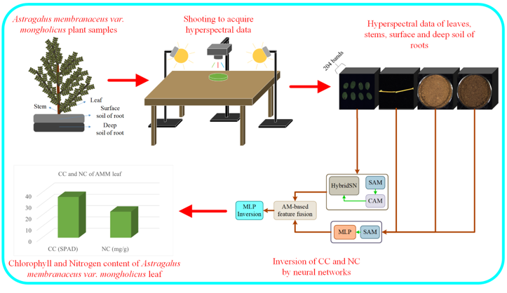
In the context of smart agriculture, accurately estimating plant leaf chemical parameters is crucial for optimizing crop management and improving agricultural yield. Hyperspectral imaging, with its ability to capture detailed spectral information across various wavelengths, has emerged as a powerful tool in this regard. However, the complex and high-dimensional nature of hyperspectral data poses significant challenges in extracting meaningful features for precise estimation. To address this challenge, this study proposes an end-to-end estimation network for multiple chemical parameters of Astragalus leaves based on attention mechanism (AM) and multivariate hyperspectral features (AM-MHENet). We leveraging HybridSN and multilayer perception (MLP) to extract prominent features from the hyperspectral data of Astragalus membranaceus var. mongholicus (AMM) leaves and stems, as well as the surface and deep soil surrounding AMM roots. This methodology allows us to capture the most significant characteristics present in these hyperspectral data with high precision. The AM is subsequently used to assign weights and integrate the hyperspectral features extracted from different parts of the AMM. The MLP is then employed to simultaneously estimate the chlorophyll content (CC) and nitrogen content (NC) of AMM leaves. Compared with estimation networks that utilize only hyperspectral data from AMM leaves as input, our proposed end-to-end AM-MHENet demonstrates superior estimation performance. Specifically, AM-MHENet achieves an R2 of 0.983 with an RMSE of 0.73 for the estimation of CC in AMM leaves. For NC estimation, AM-MHENet achieves an R2 value of 0.977 with an RMSE of 0.27. These results underscore AM-MHENet’s effectiveness in significantly enhancing the accuracy of both CC and NC estimation in AMM leaves. Moreover, these findings indirectly suggest a strong correlation between the development of AMM leaves and stems, as well as the surface and deep soil surrounding the roots of AMM, and directly highlight the ability of AM to effectively focus on the relevant spectral features within the hyperspectral data. This findings from this study could offer valuable insights into the simultaneous estimation of multiple chemical parameters in plants, thereby making a contribution to the existing body of research in this field.
Keywords:
Astragalus membranaceus var. mongholicus
; Chemical parameters
; Hyperspectral estimation
; Attention mechanism
; Deep network
1. Introduction
Astragalus membranaceus var. mongholicus (AMM) is a traditional bulk medicinal herb in China [1], that is cultivated predominantly in regions such as Gansu, Shanxi, and Inner Mongolia [2]. It is a perennial herb species of the Astragalus genus within the legume family, renowned for its antitumor and blood sugar-lowering properties, and has significant economic and medicinal value [3,4]. In recent years, with increasing attention to health, the demand for Chinese (Mongolian) medicinal herbs has increased, leading to an expansion in the cultivation area of AMM [5,6]. However, the growth of AMM is influenced by factors such as fertilizers, pesticides, and pests. Failure to identify and address these issues promptly can adversely affect the yield and quality of AMM [7,8]. Moreover, there is currently limited research on the rapid monitoring of AMM growth. Therefore, it is crucial to establish a rapid monitoring model for the growth conditions of AMM.
Plant leaves are the primary site of photosynthesis [9]. Chlorophyll, as a photosynthetic pigment in higher plants [10], may directly reflect the strength of photosynthesis and health of the plant [11,12,13,14]. It is an important physiological indicator for evaluating plant growth and is closely related to crop yield and quality [15,16,17]. Nitrogen is an essential element for plant growth and quality [18]. It provides important support for plant photosynthesis, protein synthesis, carbohydrate synthesis, and carbon-nitrogen metabolism, greatly affecting plant growth, yield, and quality [19,20,21]. The timely determination of plant chlorophyll content (CC) and nitrogen content (NC), followed by the application of an appropriate amount of nitrogen fertilizer at the right time, is extremely important for achieving high yields with less nitrogen fertilizer [22]. Therefore, the rapid and precise monitoring of CC and NC in plant leaves is key to accurately assessing crop growth and health status.
Traditional methods for estimating leaf CC and NC are typically destructive, and involve laborious, slow, and narrowly scoped detection processes, which present challenges for large-scale monitoring [23,24,25]. Additionally, these methods generate toxic chemicals that can negatively impact the environment [26]. Hyperspectral imaging technology, an effective integration of spectral analysis and image processing techniques, facilitates precise, rapid, and nondestructive identification of both the internal and external characteristics of the subject under study [27]. This technology has found extensive applications in agricultural monitoring [28,29]. Eshkabilov et al. developed five classification and regression models using hyperspectral technology to model lettuce growth. The results demonstrated that the hyperspectral-based models achieved high accuracy in classifying lettuce and estimating nutrient concentrations [30]. Yuan et al. first applied the Savitzky-Golay algorithm to smooth the raw spectra, followed by several preprocessing algorithms. Various feature selection methods were then employed to identify characteristic spectral bands, and multiple regression models were used to estimate the SPAD values of cotton leaves. The results showed that spectral preprocessing improved the correlation between the selected bands and SPAD values. The model based on CARS-selected bands demonstrated higher estimation accuracy, and the multifactor model outperformed the single-factor model in terms of estimation accuracy [31].
However, current studies lack a large-scale end-to-end hyperspectral inversion model that simultaneously uses leaf, stem, and soil data as inputs to estimate multiple chemical parameters of plant leaves. To address this gap, this study employs hyperspectral imaging technology to collect hyperspectral data of AMM leaves, stems, the surface and deep soil surrounding AMM roots. The processes of hyperspectral feature extraction and leaf chemical parameter estimation are integrated into a end-to-end deep learning network.
Considering the distinct hyperspectral characteristics of leaves, stems, and soil, a multi-branch feature extraction network module was designed, incorporating enhancements from the spatial attention mechanism (SAM) and channel attention mechanism (CAM) [32] to improve feature extraction. Additionally, a feature fusion network module improved by an attention mechanism (AM) [33] was developed to integrate these extracted hyperspectral features, which were then used to estimate the CC and NC of AMM leaves simultaneously. The proposed end-to-end estimation network, based on the AM and multivariate hyperspectral features (AM-MHENet), fully leverages the hyperspectral data of AMM leaves, stems, and the soil surrounding AMM roots.
2. Materials and Methods
2.1. Data Collection
2.1.1. Sample Collection
The AMM samples for this study were collected in mid-October 2023 from the Guyang AMM research demonstration base (,), a dry herb planting region in China. Figure 1 shows the geographical location of the AMM harvesting area. The AMM research demonstration base is located in Guyang County, in the western section of Daqing Mountain on the Inner Mongolia Plateau. This region features a typical ’plateau basin’ terrain with excellent heat accumulation, providing highly favorable conditions for the growth of AMM.
To assess the spatial variability of soil properties and the growth performance of AMM under different soil and environmental conditions, we employed a grid distribution method to collect AMM plant samples and soil surrounding AMM roots. Figure 2 shows a diagram of the samples. The collected plants and soil samples were sealed, labeled, and the geographical coordinates of the collection sites were recorded before transportation to the laboratory.
2.1.2. Hyperspectral Data Acquisition
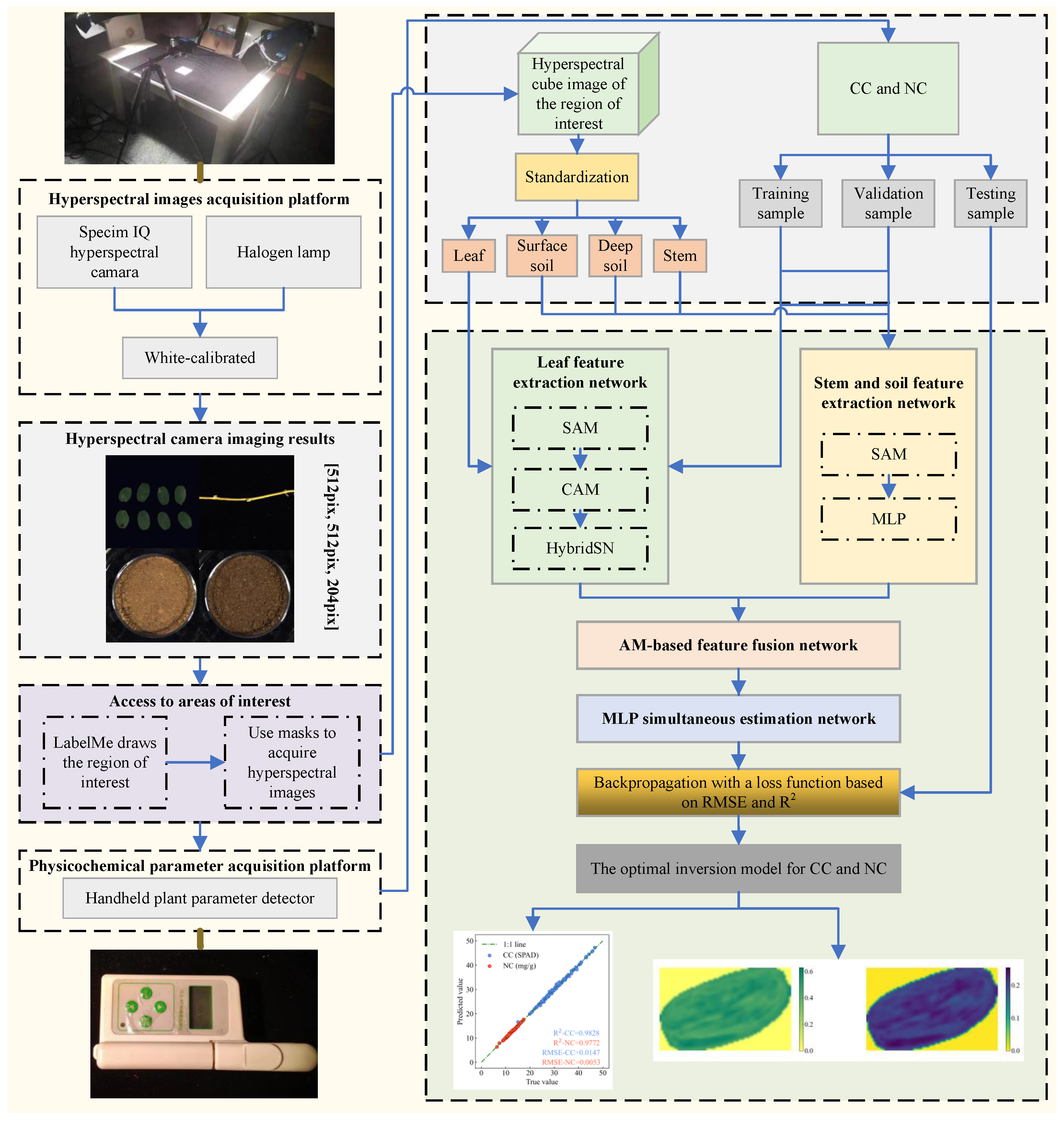
The hyperspectral data of AMM leaves, stems, and the surface and deep layers surrounding AMM roots were captured via a new handheld Specim IQ hyperspectral camera. Detailed parameters and settings of the hyperspectral camera are provided in Appendix A.1.
To mitigate the influence of outdoor sunlight angles and obstructions from objects such as clouds on illumination intensity, shooting was conducted in a dark room to minimize external light interference. Two halogen lamps provided focused lighting. Once the angle of the halogen lamps was set, it remained fixed throughout the data collection to minimize errors due to lighting variations. Figure 3 shows the scene of hyperspectral data acquisition.
During the imaging process, a standard whiteboard was initially photographed, and subsequently, the whiteboard correction function integrated into the hyperspectral camera was employed to mitigate the effects of uneven light intensity. Figure 4 shows the false color data of the hyperspectral data of the harvested AMM leaves, stems, and surface and deep soil surrounding AMM roots.
2.1.3. Preprocessing of Hyperspectral Data
Hyperspectral data contain both valuable information about the detected samples and irrelevant information such as the background. Therefore, extracting the region of interest from these data is essential. In this study, regions of interest were delineated via ’LabelMe’, followed by multiplication of the obtained masks with hyperspectral data to extract hyperspectral data within the regions of interest. Figure 5 shows a diagram of the region of interest. By extracting the region of interest, the scope of attention can be narrowed, which reduces the computational load of the data feature extraction and estimation processes, thereby increasing the estimation efficiency.
Figure 6 shows the spectral curves corresponding to the regions of interest extracted from the hyperspectral data of AMM leaves, stems, and the surface and deep soil surrounding AMM roots. This shows that the overall trends of the spectral curves of the AMM leaves, stems, and soil surrounding AMM roots are different, with significant differences in reflected light intensity at different wavelengths.
To expedite the model training process, prevent issues such as gradient explosion or vanishing, and improve the model’s generalization ability and numerical stability, normalizing hyperspectral data is essential. In this study, we employ the z-score standardization method for normalization purposes. The formula of the z-score is shown in Equation (1):
where x represents the spectral value, is the spectral mean, is the spectral variance, and is the normalized spectral value.
2.1.4. CC, NC Measurement
The CC and NC of AMM leaves were measured via a handheld plant parameter detector. Besides, during the process of capturing measurement errors, six measurements were taken separately on each leaf, and the average value was calculated and used as the parameter indicator. The average value was used as the parameter indicator. Moreover, during the process of capturing the hyperspectral data of the leaves, measurements of the CC and NC of AMM leaves were conducted. A total of 1431 datasets were collected in this study. Figure 7 shows the histograms of the CC and NC distributions of the leaf samples.
2.1.5. Data Augmentation and Dataset Segmentation
To solve the problem of insufficient data for training via deep learning, the number of datasets needs to be expanded via data augmentation methods. Since the original hyperspectral data contain spatial information, we employed traditional image dataset augmentation techniques, such as rotation and mirroring, to expand the dataset. The size of the dataset after data augmentation is 11,448.
Eight percent of the 11448 AMM leaf samples along with their corresponding stem, surface, and deep soil samples, totaling 9152 samples, were allocated to the training set. Ten percent of the samples, amounting to 1144 samples, were assigned to the validation set, and the remaining 10%, totaling 1152 samples, were designated the test set.
2.2. Overall Structure of AM-MHENet
Figure 8 shows the diagram of AM-MHENet. The model inputs consisted of hyperspectral data from AMM leaves, stems, and the surface and deep soil surrounding AMM roots. The model outputs are the CC and NC in the leaves of the AMM. After features from hyperspectral data of AMM leaves, stems, and the surface and deep soil surrounding AMM roots are extracted via a HybridSN [34] feature extraction network module enhanced by the SAM and CAM, as well as MLP feature extraction network modules [35] improved by the SAM, the separately extracted features are integrated via an AM. Finally, an MLP simultaneous estimation network module is employed to achieve simultaneous estimation results of CC and NC in AMM leaves.
2.3. AM-Improved Feature Extraction Network Module
2.3.1. HybridSN-Based Leaf Feature Extraction Network Module
This study uses an improved HybridSN network module to extract features from leaf hyperspectral data. Given that the primary objective of this study is to estimate the CC and NC of AMM leaves, the classification module of HybridSN has been omitted. Instead, enhancements have focused on refining the feature extraction module of HybridSN to extract the characteristics of AMM leaves.
Given the significant redundancy in hyperspectral data, our approach employs SAM to enhance spatial information sensitive to CC and NC, aiming to extract more discerning spatial features. The hyperspectral data features enhanced by the SAM are subsequently refined via CAM to amplify spectral information that is particularly sensitive to CC and NC. Finally, the hyperspectral features processed by the CAM are input into the HybridSN feature extraction module for further feature extraction, resulting in an improved HybridSN feature extraction module. Figure 9 illustrates the structure of the improved HybridSN feature extraction module.
Compared with the original HybridSN feature extraction module, the improved version incorporates the SAM and CAM to improve the extraction of spatial and spectral information from AMM leaves. Initially, the SAM processes the input features to amplify spatial characteristics crucial for the estimation results. The CAM subsequently enhances spectral bands that are particularly relevant to estimation outcomes Finally, the HybridSN feature extraction module further refines spatial-spectral joint features and spatial characteristics. The network structure and specific parameters of the improved HybridSN feature extraction module are provided in Appendix B.1.
2.3.2. MLP-Based Stem and Soil Feature Extraction Network Module
In this study, improved MLP network module are employed to extract features from the hyperspectral data of stems and soil. Traditional MLP networks result in a loss of spatial information from the hyperspectral data of AMM stems and the surface and deep soil surrounding AMM roots, retaining only spectral information. To fully leverage the spatial information in hyperspectral data without increasing model complexity, the hyperspectral data of stems and soil are initially processed via SAM to emphasize spatial features. The hyperspectral data enhanced by the SAM are then input into the MLP network module for further feature extraction, which improves the performance of the network module. Figure 10 shows the structural diagram of the improved MLP network module.
Compared with the original MLP network, the enhanced version incorporates SAM, enhancing the ability to extract spatial information from the hyperspectral data of AMM stems and surface and deep soil surrounding AMM roots. The hyperspectral data features of the AMM stems and surface and deep soil surrounding AMM roots are initially processed through SAM, emphasizing spatial characteristics crucial for estimation results. These features subsequently undergo further extraction by the MLP network module. The network structure and specific parameters of the improved MLP feature extraction module are provided in Appendix B.2.
2.4. Estimation Algorithm for CC and NC in AMM Based on Multivariate Hyperspectral Feature Fusion
Integrating feature information from hyperspectral data of AMM leaves, stems, and surface and deep soil surrounding AMM roots can increase the accuracy and reliability of estimation, enabling more precise estimation of CC and NC in AMM leaves. Figure 11 shows the process flow of the estimation algorithm based on multivariate hyperspectral feature fusion for CC and NC in AMM leaves.
The input hyperspectral data of AMM leaves, stems, and surface and deep soil surrounding AMM roots are processed through dedicated leaf and stem-soil feature extraction network modules, respectively. This results in distinct features for the leaves, stems, and soil. An AM is subsequently used to integrate the extracted features. Finally, a simultaneous estimation network module is employed to simultaneously estimate the CC and NC of the AMM leaves.
2.4.1. AM-Based Multivariate Hyperspectral Feature Fusion Algorithm
By employing an AM-based network module, different weights are assigned to the feature information from the hyperspectral data of AMM leaves, stems, and surface and deep soil surrounding AMM roots. This facilitates the fusion of multivariate input features, fully leveraging the hyperspectral data from the leaves, stems, and surface and deep soil surrounding AMM roots to simultaneously estimate the CC and NC of the leaves. Figure 12 shows the multivariate hyperspectral feature fusion network module structure based on the AM.
The structure of the multivariate hyperspectral feature fusion network module based on the AM resembles that of the CAM structure, which is primarily composed of nonlinear layers. The key distinction lies in the input feature dimensions: the CAM processes three-dimensional input features, whereas this feature fusion network module handles two-dimensional input features. Furthermore, after pooling, the CAM compresses its input features via nonlinear transformations and subsequently restores them to their original length. In contrast, this feature fusion network module initially expands its input features with nonlinear transformations after pooling and then restores them to their original dimensions. The structure and specific parameters of the multivariate hyperspectral feature fusion network module based on the AM are provided in Appendix B.3.
2.4.2. Simultaneous Estimation Algorithm Based on Integrated Features for CC and NC
After the feature information from the hyperspectral data of AMM leaves, stems, and surface and deep soil surrounding AMM roots is integrated, an MLP network module is used to simultaneously estimate the CC and NC of the leaves. Figure 13 shows the structural diagram of the MLP simultaneous estimation network module.
This network module primarily comprises linear components. Initially, it transforms two-dimensional integrated features into one-dimensional features. Subsequently, it performs nonlinear mapping via two dense modules. Finally, it employs a linear module to estimate the CC and NC of AMM leaves. The structure and specific parameters of the MLP simultaneous estimation network module are provided in Appendix B.4.
2.5. MSE-R2 Loss Function
Hyperspectral estimation models commonly use and as evaluation metrics [36,37,38]. The formula for is shown in Equation (2):
where is the predicted value of the estimation model; is the real label; and n is the number of samples. The closer the value is to 0, the better the model; the larger the value is, the worse the model.
The formula for is shown in Equation (3):
where is the average value of the actual labels. The value of typically ranges from 0 to 1. The closer the value is to 1, the better the model. Conversely, the smaller the value is, the worse the model.
The training process of deep learning is primarily conducted through the backpropagation algorithm, which calculates the error between the network’s predicted values and the true values. This error signal is then propagated backward to update the network parameters, optimizing the network’s performance. In this process, the choice of loss function is also crucial.
For regression models, such as hyperspectral estimation, the is commonly used as the loss function [39]. Hyperspectral estimation typically employs the and as evaluation metrics. The formula of the relationship between and is shown in Equation (4):
To directly optimize both and during the training process of deep learning, and to ensure that the predicted values are as close as possible to the true values, making the loss function approach zero, this study has designed the MSE-R2 loss. The formula of MSE-R2 loss is shown in Equation (5):
where L is the MSE-R2 loss; is the predicted value of the estimation model; is the real label; n is the number of samples; and is the average value of the actual labels.
2.6. Technical Roadmap
In this study, 1431 samples of AMM leaves, along with their corresponding stems, surface and deep soil surrounding AMM roots, were selected as research objects. The hyperspectral data of these samples as well as the CC and NC data in the leaf samples were obtained. The hyperspectral data were first white balanced, followed by extraction of the original spectral data from the regions of interest. The hyperspectral data were subsequently standardized, and the dataset was subsequently partitioned into training, validation, and test sets. The improved HybridSN and MLP, which are enhanced by AM, were employed to extract features from hyperspectral data. Subsequently, an AM-based feature fusion algorithm integrated these features, and an MLP simultaneous estimation algorithm was applied to estimate CC and NC in AMM leaves. The model was trained via backpropagation with a loss function designed based on and for optimization. Finally, the trained model was applied to estimate the CC and NC in the test set of AMM leaves. Detailed technical roadmap can be found in Appendix C.
3. Results
3.1. Experimental Environment and Parameter Settings
AM-MHENet was trained on a Windows Server 2022 Datacenter system. The hardware configurations of the system are provided in Appendix A.2. For a comprehensive comparison between the proposed end-to-end AM-MHENet and other models, hyperparameters were optimized via the ’Adam’ optimizer. The initial learning rate was set to 0.001, with a batch size of 32 and a total of 300 epochs.
The application of the cosine annealing algorithm to dynamically adjust the learning rate can significantly enhance model convergence, thereby improving estimation accuracy. The formula for the cosine annealing learning rate is shown in Equation (6):
where is the current learning rate; is the set minimum learning rate; is the set maximum learning rate; is the current cycle; and is the set maximum training cycle.
3.2. Training Results
In the test set, AM-MHENet’s estimation of AMM leaf CC achieved an of 0.983 and an of 0.73. For NC, the estimation achieved an of 0.977 and an of 0.27. Figure 14 shows the scatter plot of the AM-MHENet estimation results for CC and NC in the partial AMM leaf samples from the test set. The scatter points closely align with the 1:1 line, suggesting high accuracy in estimating CC and NC through the AM-MHENet.
Figure 15 shows the comparison bar chart of the predicted values versus the true values for CC and NC in AMM leaves within the partial test set. The results indicate that the model’s estimation error for CC can be controlled within 1, while the estimation error for NC is kept within 0.4.
Figure 16 shows the heatmap of the absolute values of the average CAM weights for the leaves in the test set. This indicates that the absolute values of most band weights fall within the range of [0.2, 0.8], whereas the bands that significantly impact the estimation of CC and NC are located primarily at approximately 550, 700, and 920 nm. This suggests that the CAM effectively utilizes the spectral information from hyperspectral data.
Figure 17 shows a 3D scatter plot of the AM-MHENet estimation results in the partial test set. In the plot, the blue surface represents the plane formed by extending a line fitted with the CC value x and NC value y in the sample dimension.
The proximity of all the points to the blue plane suggests a discernible linear relationship between CC and NC. The linear equation fitted for CC and NC is presented in Equation (7):
As shown in Figure 18, different colors (yellow, green, and blue) and color depths represent the CC and NC of AMM leaves. Owing to the small size of AMM leaves (5–10 mm in length and 3–5 mm in width), the differences in CC and NC across different parts of a single leaf are minimal.
Figure 19 shows the predicted and measured values of CC and NC in partial AMM leaves from the test set, with standard deviations represented as error bars. An analysis of the mean and standard deviation of each pixel in the estimation data reveals that most of the predicted values closely match the measured values, demonstrating a strong correlation. This finding indicates that using hyperspectral imaging technology to construct CC and NC distribution maps for AMM leaves is effective. This method enables rapid and accurate acquisition of CC and NC at a small-area scale, providing a theoretical basis for future plant growth monitoring.
3.3. Comparative Experiment
This study designs multiple sets of experiments for comparative analysis to verify the superiority and reliability of the AM-MHENet. To validate the effectiveness of integrating the feature extraction process with the parameter estimation process within the end-to-end network, traditional feature extraction algorithms such as autoencoder (AE) [40], principal component analysis (PCA) [41], and the genetic algorithm (GA) [42] are employed. Finally, the features extracted via these methods are input into an MLP simultaneous estimation network module for estimation.
Figure 20 shows a scatter plot of the CC and NC estimation results for AMM leaves in the partial test set via different feature extraction methods. The findings indicate that the estimation results for CC and NC from the end-to-end network, which integrates both feature extraction and parameter estimation processes into a single model (as shown in Figure 14), are closer to the 1:1 line compared with models that separate these processes. This suggests that integrating these processes enhances the extraction of crucial feature information from the original hyperspectral data, thereby improving the accuracy of estimation results aligned with measured values.
To validate the effectiveness of the feature extraction network module enhanced by AM, ablation experiments were conducted. Three control groups were established—one without SAM and CAM, one without SAM only, and one without CAM only—for training and estimation. Figure 21 presents the results of the AM ablation experiment on the test set. The findings indicate that, compared with the estimation model utilizing feature extraction network modules not enhanced by the CAM or SAM, the estimation results of AM-MHENet (as shown in Figure 14) are closer to the 1:1 line. This underscores that the SAM and CAM effectively leverage spatial and spectral information from hyperspectral data.
Figure 22 shows a scatter plot of CC and NC estimation results for AMM leaves in the partial test set under different feature fusion methods. The results demonstrate that the estimation results obtained via a multi-input feature fusion network module based on AM (as shown in Figure 14) are closer to the 1:1 line than methods that use only ’add’ or ’concatenate’. This underscores the ability of the AM-based multi-input feature fusion network module to evaluate the influence of various input features on the estimation task. It effectively allocates weights to different input features, thereby leveraging them comprehensively to enhance the model’s estimation accuracy.
To validate the efficacy of simultaneous estimation for CC and NC, an ablation experiment was conducted. The dual-output structure of the AM-MHENet was modified to a single-output structure, and separate estimation models were trained with CC and NC as individual outputs to estimate each parameter separately.
Figure 23 shows the scatter plot results of separate estimation results for CC and NC in the partial test set. The findings indicate that simultaneous estimation results for CC and NC (as shown in Figure 14) are closer to the 1:1 line than separate estimations are. This experiment indirectly confirms the correlation between CC and NC. The study suggests that, owing to the mutual influence of CC and NC fitting during the AM-MHENet training process, the ability to avoid local optima is enhanced, thereby improving the estimation accuracy. Moreover, this approach can increase the efficiency of the model in simultaneously estimating CC and NC in AMM leaves.
To validate the efficacy of integrating multivariate hyperspectral characteristics from AMM leaves, stems, and the surface and deep soil surrounding AMM roots, ablation experiments were conducted. The estimation models were designed using only AMM leaves as input, both AMM leaves and stems, and both AMM leaves and soil surrounding AMM roots, and these models were then compared against AM-MHENet.
Figure 24 shows the results of ablation experiments with various input combinations in the partial test set. The findings indicate that the AM-MHENet estimation results (as shown in Figure 14) align more closely with the 1:1 line than do those of the models that use only leaves as inputs or other input combinations. This comparative experiment indirectly demonstrated the influence of stems and the surface and deep soil surrounding AMM roots on the development of AMM leaves, thereby impacting their CC and NC. This finding illustrates that AM-MHENet effectively extracts meaningful features from the hyperspectral data of AMM stems and the surface and deep soil surrounding AMM roots in combination with the hyperspectral data of AMM leaves to accurately estimate their CC and NC.
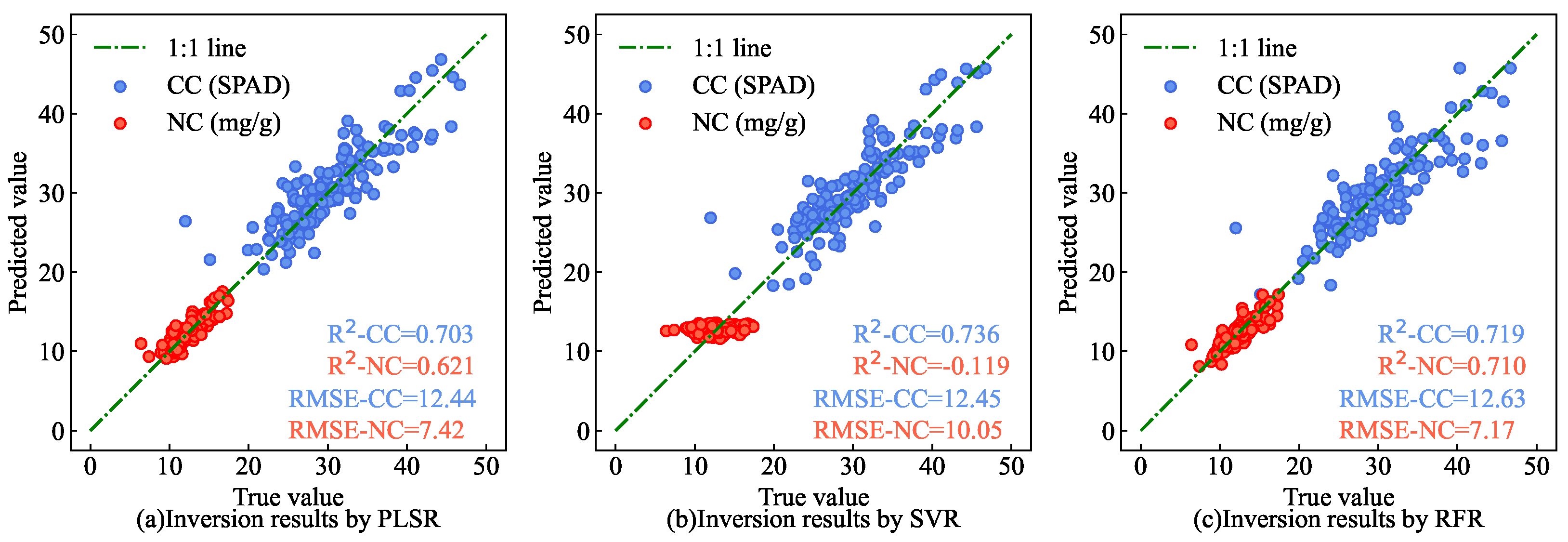
The current mainstream models for leaf CC and NC estimation based on hyperspectral data include support vector regression (SVR) [43], random forest regression (RFR) [44], and partial least squares regression (PLSR) [45]. Figure 25 shows the scatter plots of the CC and NC results for AMM leaves under different estimation models in the partial test set. The results show that the estimation results of AM-MHENet for the test set data (as shown in Figure 14) are closer to the 1:1 line than those of the SVR, RFR, and PLSR methods are. This shows that, compared with traditional hyperspectral estimation models, AM-MHENet not only simultaneously estimates the CC and NC of AMM leaves but also achieves higher estimation efficiency and accuracy.
The experimental results show that, compared to other models, the end-to-end deep learning network—enhanced with AM and integrating multivariate hyperspectral features—yields the best results for simultaneously estimating CC and NC in AMM leaves.
4. Discussion
With the increasing demand for Chinese (Mongolia) medicinal herbs such as AMM, establishing a rapid monitoring model for the growth conditions of AMM by estimating the CC and NC of its leaves is crucial. The AM-MHENet model proposed in this study effectively addresses the limitations of traditional methods for monitoring leaf chemical parameters. In contrast to conventional approaches, this model integrates hyperspectral data from AMM leaves, stems, and soil, allowing for the simultaneous estimation of CC and NC in the leaves. Specifically, the AM-MHENet model achieved an of 0.983 and an of 0.73 for CC estimation, and an of 0.977 and an of 0.27 for NC estimation. These results demonstrate the superior accuracy and reliability of the AM-MHENet model.
Traditional hyperspectral-based algorithms for estimating leaf chemical parameters typically separate the processes of feature extraction and chemical parameter estimation [46,47,48]. Although this method has been successful, its performance is limited by domain-specific, hand-engineered features and processing inefficiencies, which may alter the original spectral patterns and reduce its overall effectiveness [49]. In contrast, the AM-MHENet model proposed in this study integrates hyperspectral feature extraction and leaf chemical parameter evaluation within a end-to-end deep learning network. This integrated approach enhances the extraction of hyperspectral features pertinent to leaf chemical parameters, thereby improving the model’s accuracy in parameter assessment.
The high spatial and spectral resolution of hyperspectral data enables a comprehensive analysis of stem development and soil nutrient content [50,51,52,53,54,55]. However, existing hyperspectral-based models for estimating leaf chemical parameters typically use only leaf hyperspectral images as input [56,57,58], often neglecting the impact of stems and soil on plant leaf development. The AM-MHENet model proposed in this study addresses this gap by integrating hyperspectral data from leaves, stems, and soil. This integration enables the model to not only process leaf hyperspectral data but also consider the effects of stems and soil, significantly enhancing the accuracy of the estimation.
The high accuracy of the AM-MHENet model is primarily attributed to its end-to-end design, which simplifies the process by integrating feature extraction and estimation into a unified framework. This design enables joint training and direct output, thereby improving both efficiency and accuracy [59]. Additionally, the CC and NC in plant leaves are influenced not only by the leaves themselves but also by the plant’s stems and surrounding soil [60,61]. The model’s multi-branch network structure allows it to simultaneously process and integrate data from these various sources, thereby fully utilizing hyperspectral information from leaves, stems and soil. This integrated consideration significantly improves the accuracy of CC and NC estimation, resulting in superior performance of the model in practical applications.
Although the AM-MHENet model demonstrates strong performance in this study, it has certain limitations. For example, the model’s deep learning architecture involves numerous parameters, requiring a substantial amount of data for adequate parameter fitting. Additionally, the need to simultaneously collect leaf, stem, and soil samples adds complexity to the data acquisition process, which may further increase the challenges associated with the model’s practical application.
Future research could expand the application scope of the AM-MHENet model by assessing additional chemical parameters, such as phosphorus and potassium, which are critical to plant development. Additionally, exploring the model’s performance across various crops and environmental conditions would help to validate its generalizability and adaptability. Further studies could also consider integrating the model with other types of sensor data to enhance prediction accuracy and reliability.
The AM-MHENet model proposed in this study demonstrates significant practical potential. It can simultaneously estimate multiple chemical parameters, making it well-suited for monitoring plant health and nutritional status in agricultural management. By providing precise estimation of CC and NC, the model can assist agricultural producers in optimizing fertilization strategies, thereby enhancing crop yield and quality. Furthermore, the model’s ability to integrate soil factors increases its flexibility and effectiveness across different soil types.
5. Conclusions
This study addresses the precise estimation of the chemical parameters of plant leaves in smart agriculture by designing an end-to-end AM-MHENet. The primary aim is to achieve accurate estimation of CC and NC in AMM leaves. The main contributions and research conclusions are as follows:
- This study focused on the chemical parameters of 1431 AMM leaf samples from Guyang County, Baotou city, Inner Mongolia Autonomous Region. Using measured hyperspectral data of AMM leaves, stems, and surface and deep soil surrounding AMM roots, as well as the CC and NC of the leaves, we established an estimation model with the leaves, stems, and surface and deep soil surrounding AMM roots as inputs and the CC and NC of the leaves as outputs. A feature extraction network module based on HybridSN and MLP, improved by SAM and CAM, was employed to capture the most significant features in the data. AM was used to integrate multiple hyperspectral features, constructing a simultaneous estimation model. The model was trained via the MSE-R2 loss function. Ultimately, by integrating multivariate hyperspectral features from leaves, stems, and surface and deep soil surrounding AMM roots, we accurately estimated the CC and NC of AMM leaves.
- Compared with traditional hyperspectral feature extraction algorithms, the AM-enhanced feature extraction network module significantly improves the extraction of effective features from hyperspectral data. Additionally, the multi-feature fusion network offers higher accuracy and estimation efficiency than single-input, single-output hyperspectral estimation models do. Moreover, the deep learning-based estimation model provides greater stability than conventional estimation models do. Furthermore, integrating feature extraction and chemical parameter estimation within the end-to-end network is more efficient than traditional models that separate these processes.
Author Contributions
Conceptualization, Z.X.; methodology, Y.Z. and Z.X.; software, Y.Z.; validation, Z.X. and T.B.; formal analysis, Y.Z.; investigation, Z.X.; resources, Z.X. and T.B.; data curation, Y.Z.; writing—original draft preparation, Y.Z.; writing—review and editing, Y.Z., Z.X., T.B. and T.F.; visualization, Y.Z. and Z.X.; supervision, Z.X., T.B. and T.F.; project administration, Z.X. and T.B.; funding acquisition, Z.X. and T.B. All authors have read and agreed to the published version of the manuscript.
Funding
This research was funded by the Inner Mongolia Autonomous Region Science and Technology Program grant number 2021GG0345, the Natural Science Foundation of Inner Mongolia Autonomous Region grant number 2021MS06020, the Inner Mongolia Natural Science Foundation grant number 2024QN04013 and the Green Agriculture and Animal Husbandry Program grant number 2022XYJG00001-14.
Data Availability Statement
The dataset supporting the conclusions of this article is available in the github repository, https://github.com/zyl-mwy/MPAINet/blob/main/README.md. The code supporting the conclusions of this article is available in the github repository, https://github.com/zyl-mwy/MPAINet/tree/main.
Acknowledgments
We acknowledge the support received from the Inner Mongolia Autonomous Region Science and Technology Program (2021GG0345) and the Natural Science Foundation of Inner Mongolia Autonomous Region (2021MS06020). It is also supported by the Inner Mongolia Natural Science Foundation (2024QN04013) and the Green Agriculture and Animal Husbandry Program (2022XYJG00001-14).
Conflicts of Interest
The authors declare no conflicts of interest.
Abbreviations
The following abbreviations are used in this manuscript:
| AM | attention mechanism |
| MLP | multilayer perception |
| AMM | Astragalus membranaceus var. mongholicus |
| CC | chlorophyll content |
| NC | nitrogen content |
| SAM | spatial attention mechanism |
| CAM | channel attention mechanism |
| AE | autoencoder |
| PCA | principal component analysis |
| GA | genetic algorithm |
| SVR | support vector regression |
| RFR | random forest regression |
| PLSR | partial least squares regression |
| AM-MHENet | estimation network for multiple chemical parameters of Astragalus leaves based on attention mechanism |
Appendix A Hardware specifications
Appendix A.1. Specification of the hyperspectral camera
Table A1 lists the specification of the hyperspectral camera. The Specim IQ featured 204 spectral bands ranging from 400 to 1000 nm, covering visible light to near-infrared wavelengths, with a sampling interval of 3 nm. The data obtained from the Specim IQ hyperspectral camera consisted of hyperspectral cube data (.dat format) with high spatial and spectral resolutions.

Table A1.
Characterization of the Specim IQ
| Parameter | Specification |
|---|---|
| Detector specification | CMOS |
| Spectral region | 400-1000 nm |
| Sample interval | 3 nm |
| Channels | 204 |
| Image resolution | 512x512 pix |
| Data output bit depth | 12 bit |
Appendix A.2. Hardware configuration of the system
Table A2 list the hardware configurations of the system.
Table A2.
Hardware configuration of the system
| Hardware Component | Specification |
|---|---|
| Central Processing Unit | AMD Ryzen Threadripper PRO 3945WX |
| Graphics Processing Unit | NVIDIA RTX A4000 |
| Video Random Access Memory | 16 G |
| Random Access Memory | 128 G |
Appendix B Network structure and specific parameters
Appendix B.1. Improved HybridSN feature extraction module
Table A3 lists the network structure and specific parameters of the improved HybridSN feature extraction module.
Table A3.
Network structure and specific parameters of the improved HybridSN feature extraction module
Table A3.
Network structure and specific parameters of the improved HybridSN feature extraction module
| Module | Layer (type) | Output shape | Number of parameters |
|---|---|---|---|
| Input | Input Layer | (-1,1,204,16,16) | 0 |
| SAM 1 | AdapAvgPool1d 2 | (-1,1,16,16) | 0 |
| AdapMaxPool1d 3 | (-1,1,16,16) | 0 | |
| Concatenate | (-1,2,16,16) | 0 | |
| Conv2d 4 | (-1,1,16,16) | 98 | |
| Sigmoid | (-1,1,16,16) | 0 | |
| CAM 5 | AdapAvgPool2d 6 | (-1,204,1,1) | 0 |
| Linear | (-1,12) | 2448 | |
| ReLU 7 | (-1,12) | 0 | |
| Linear | (-1,204) | 2448 | |
| Sigmoid | (-1,204) | 0 | |
| HybridSN | Conv3d 8 | (-1,8,198,14,14) | 5 776 |
| ReLU | (-1,8,198,14,14) | 0 | |
| Conv3d | (-1,16,194,12,12) | 13 856 | |
| ReLU | (-1,16,194,12,12) | 0 | |
| Conv3d | (-1,32,192,10,10) | 3 539 008 | |
| ReLU | (-1,32,192,10,10) | 0 | |
| Conv2d | (-1,64,8,8) | 98 | |
| ReLU | (-1,64,8,8) | 0 |
1 Spatial Attention Mechanism; 2 1-dimensional Adaptive Average Pooling; 3 1-dimensional Adaptive Maximum Pooling; 4 2-dimensional Convolution; 5 Channel Attention Mechanism; 6 2-dimensional Adaptive Average Pooling; 7 Rectified Linear Unit; 8 3-dimensional Convolution.
Appendix B.2. Improved MLP feature extraction module
Table A4 lists the network structure and specific parameters of the improved MLP feature extraction module.
Table A4.
Network structure and specific parameters of the improved MLP feature extraction module
| Module | Layer (type) | Output shape | Number of parameters |
|---|---|---|---|
| Input | Input Layer | (-1,1,204,16,16) | 0 |
| SAM | AdapAvgPool1d | (-1,1,16,16) | 0 |
| AdapMaxPool1d | (-1,1,16,16) | 0 | |
| Concatenate | (-1,2,16,16) | 0 | |
| Conv2d | (-1,1,16,16) | 98 | |
| Sigmoid | (-1,1,16,16) | 0 | |
| MLP | AdapAvgPool2d | (-1,204,1,1) | 0 |
| Linear | (-1,1024) | 209 920 | |
| ReLU | (-1,1024) | 0 | |
| Linear | (-1,2048) | 2 099 200 | |
| ReLU | (-1,2048) | 0 | |
| Linear | (-1,4096) | 8 392 704 | |
| ReLU | (-1,4096) | 0 |
Appendix B.3. Multiple hyperspectral feature fusion network module based on AM
Table A5 lists the network structure and specific parameters of the multivariate hyperspectral feature fusion network module based on the AM.
Table A5.
Structure and specific parameters of the multiple hyperspectral feature fusion network module based on AM
Table A5.
Structure and specific parameters of the multiple hyperspectral feature fusion network module based on AM
| Layer (type) | Output shape | Number of parameters |
|---|---|---|
| Input Layer 1 | (-1,1,204,16,16) | 0 |
| Input Layer 2 | (-1,1,204,16,16) | 0 |
| Input Layer 3 | (-1,1,204,16,16) | 0 |
| Input Layer 4 | (-1,1,204,16,16) | 0 |
| Concatenate | (-1,4,4096) | 0 |
| AdapAvgPool1d | (-1,4,1) | 0 |
| Linear | (-1,16) | 64 |
| ReLU | (-1,16) | 0 |
| Linear | (-1,4) | 64 |
| Sigmoid | (-1,16) | 0 |
Appendix B.4. MLP simultaneous estimation network module
Table A6 shows the structure and specific parameters of the MLP simultaneous estimation network module.
Table A6.
Structure and specific parameters of MLP simultaneous estimation network module
| Layer (type) | Output shape | Number of parameters |
|---|---|---|
| Input Layer | (-1,1,204,16,16) | 0 |
| Flatten | (-1,16384) | 0 |
| Linear | (-1,256) | 4 194 560 |
| ReLU | (-1,256) | 0 |
| Linear | (-1,128) | 32 896 |
| ReLU | (-1,128) | 0 |
| Linear | (-1,2)) | 258 |
Appendix C Roadmap
The technical roadmap is illustrated in Figure A1.
Figure A1.
Technical Roadmap of this study.
References
- Bi, Y.; Bao, H.; Zhang, C.; Yao, R.; Li, M. Quality control of Radix astragali (the root of Astragalus membranaceus var. mongholicus) along its value chains. Frontiers in pharmacology 2020, 11, 562376. [Google Scholar] [CrossRef] [PubMed]
- Sun, H.; Jin, Q.; Wang, Q.; Shao, C.; Zhang, L.; Guan, Y.; Tian, H.; Li, M.; Zhang, Y. Effects of soil quality on effective ingredients of Astragalus mongholicus from the main cultivation regions in China. Ecological Indicators 2020, 114, 106296. [Google Scholar] [CrossRef]
- Zheng, Y.; Ren, W.; Zhang, L.; Zhang, Y.; Liu, D.; Liu, Y. A review of the pharmacological action of Astragalus polysaccharide. Frontiers in Pharmacology 2020, 11, 349. [Google Scholar] [CrossRef]
- Wu, X.; Huang, J.; Wang, J.; Xu, Y.; Yang, X.; Sun, M.; Shi, J. Multi-pharmaceutical activities of chinese herbal polysaccharides in the treatment of pulmonary fibrosis: Concept and future prospects. Frontiers in Pharmacology 2021, 12, 707491. [Google Scholar] [CrossRef] [PubMed]
- Fu, J.Y.; Zhang, X.; Zhao, Y.H.; Chen, D.Z.; Huang, M.H. Global performance of traditional Chinese medicine over three decades. Scientometrics 2012, 90, 945–958. [Google Scholar] [CrossRef]
- Zeyuan, Z.; Guoshuai, L.; Lingfei, W.; Yuan, C.; Xinxin, W.; Yaqiong, B.; Minhui, L. Statistical Data Mining and Analysis of Medicinal Plant Cultivation in Inner Mongolia Autonomous Region. Modern Chinese Medicine 2023, 25, 2274–2283. [Google Scholar]
- Cao, P.; Wang, G.; Wei, X.m.; Chen, S.l.; Han, J.p. How to improve CHMs quality: Enlighten from CHMs ecological cultivation. Chinese Herbal Medicines 2021, 13, 301–312. [Google Scholar] [CrossRef] [PubMed]
- Shahrajabian, M.H.; Kuang, Y.; Cui, H.; Fu, L.; Sun, W. Metabolic changes of active components of important medicinal plants on the basis of traditional Chinese medicine under different environmental stresses. Current Organic Chemistry 2023, 27, 782–806. [Google Scholar] [CrossRef]
- Deans, R.M.; Brodribb, T.J.; Busch, F.A.; Farquhar, G.D. Optimization can provide the fundamental link between leaf photosynthesis, gas exchange and water relations. Nature Plants 2020, 6, 1116–1125. [Google Scholar] [CrossRef] [PubMed]
- Peng, J.; Feng, Y.; Wang, X.; Li, J.; Xu, G.; Phonenasay, S.; Luo, Q.; Han, Z.; Lu, W. Effects of nitrogen application rate on the photosynthetic pigment, leaf fluorescence characteristics, and yield of indica hybrid rice and their interrelations. Scientific Reports 2021, 11, 7485. [Google Scholar] [CrossRef]
- Wijesingha, J.; Dayananda, S.; Wachendorf, M.; Astor, T. Comparison of spaceborne and uav-borne remote sensing spectral data for estimating monsoon crop vegetation parameters. Sensors 2021, 21, 2886. [Google Scholar] [CrossRef]
- Cao, Y.; Xu, H.; Song, J.; Yang, Y.; Hu, X.; Wiyao, K.T.; Zhai, Z. Applying spectral fractal dimension index to predict the SPAD value of rice leaves under bacterial blight disease stress. Plant Methods 2022, 18, 67. [Google Scholar] [CrossRef] [PubMed]
- Zhou, Z.; Struik, P.C.; Gu, J.; van der Putten, P.E.; Wang, Z.; Yin, X.; Yang, J. Enhancing leaf photosynthesis from altered chlorophyll content requires optimal partitioning of nitrogen. Crop and Environment 2023, 2, 24–36. [Google Scholar] [CrossRef]
- Tang, C.j.; Luo, M.Z.; Zhang, S.; Jia, G.Q.; Sha, T.; Jia, Y.C.; Hui, Z.; Diao, X.M. Variations in chlorophyll content, stomatal conductance, and photosynthesis in Setaria EMS mutants. Journal of Integrative Agriculture 2023, 22, 1618–1630. [Google Scholar] [CrossRef]
- Yue, J.; Feng, H.; Tian, Q.; Zhou, C. A robust spectral angle index for remotely assessing soybean canopy chlorophyll content in different growing stages. Plant Methods 2020, 16, 104. [Google Scholar] [CrossRef] [PubMed]
- Zhang, H.; Ge, Y.; Xie, X.; Atefi, A.; Wijewardane, N.K.; Thapa, S. High throughput analysis of leaf chlorophyll content in sorghum using RGB, hyperspectral, and fluorescence imaging and sensor fusion. Plant Methods 2022, 18, 60. [Google Scholar] [CrossRef]
- Sudu, B.; Rong, G.; Guga, S.; Li, K.; Zhi, F.; Guo, Y.; Zhang, J.; Bao, Y. Retrieving SPAD values of summer maize using UAV hyperspectral data based on multiple machine learning algorithm. Remote Sensing 2022, 14, 5407. [Google Scholar] [CrossRef]
- Luo, L.; Zhang, Y.; Xu, G. How does nitrogen shape plant architecture? Journal of experimental botany 2020, 71, 4415–4427. [Google Scholar] [CrossRef] [PubMed]
- Hucklesby, D.; Brown, C.; Howell, S.; Hageman, R. Late spring applications of nitrogen for efficient utilization and enhanced production of grain and grain protein of wheat 1. Agronomy Journal 1971, 63, 274–276. [Google Scholar] [CrossRef]
- Fu, Y.; Yang, G.; Pu, R.; Li, Z.; Li, H.; Xu, X.; Song, X.; Yang, X.; Zhao, C. An overview of crop nitrogen status assessment using hyperspectral remote sensing: Current status and perspectives. European Journal of Agronomy 2021, 124, 126241. [Google Scholar] [CrossRef]
- Zhang, X.; Liang, T.; Gao, J.; Zhang, D.; Liu, J.; Feng, Q.; Wu, C.; Wang, Z. Mapping the forage nitrogen, phosphorus, and potassium contents of alpine grasslands by integrating Sentinel-2 and Tiangong-2 data. Plant Methods 2023, 19, 48. [Google Scholar] [CrossRef]
- Li, X.; Li, L.; Liu, X. Collaborative inversion heavy metal stress in rice by using two-dimensional spectral feature space based on HJ-1 A HSI and radarsat-2 SAR remote sensing data. International Journal of Applied Earth Observation and Geoinformation 2019, 78, 39–52. [Google Scholar] [CrossRef]
- Markwell, J.; Osterman, J.C.; Mitchell, J.L. Calibration of the Minolta SPAD-502 leaf chlorophyll meter. Photosynthesis research 1995, 46, 467–472. [Google Scholar] [CrossRef] [PubMed]
- Putra, B.T.W. New low-cost portable sensing system integrated with on-the-go fertilizer application system for plantation crops. Measurement 2020, 155, 107562. [Google Scholar] [CrossRef]
- Yu, H.; Ding, Y.; Xu, H.; Wu, X.; Dou, X. Influence of light intensity distribution characteristics of light source on measurement results of canopy reflectance spectrometers. Plant Methods 2021, 17, 1–12. [Google Scholar] [CrossRef] [PubMed]
- Galvez-Sola, L.; García-Sánchez, F.; Pérez-Pérez, J.G.; Gimeno, V.; Navarro, J.M.; Moral, R.; Martínez-Nicolás, J.J.; Nieves, M. Rapid estimation of nutritional elements on citrus leaves by near infrared reflectance spectroscopy. Frontiers in plant science 2015, 6, 571. [Google Scholar] [CrossRef] [PubMed]
- Lu, Y.; Saeys, W.; Kim, M.; Peng, Y.; Lu, R. Hyperspectral imaging technology for quality and safety evaluation of horticultural products: A review and celebration of the past 20-year progress. Postharvest Biology and Technology 2020, 170, 111318. [Google Scholar] [CrossRef]
- Pascucci, S.; Pignatti, S.; Casa, R.; Darvishzadeh, R.; Huang, W. Special issue “hyperspectral remote sensing of agriculture and vegetation”, 2020.
- Xiang, S.; Jin, Z.; Li, J.; Yu, F.; Xu, T. RPIOSL: construction of the radiation transfer model for rice leaves. Plant Methods 2024, 20, 1. [Google Scholar] [CrossRef] [PubMed]
- Eshkabilov, S.; Simko, I. Assessing Contents of Sugars, Vitamins, and Nutrients in Baby Leaf Lettuce from Hyperspectral Data with Machine Learning Models. Agriculture 2024, 14, 834. [Google Scholar] [CrossRef]
- Yuan, X.; Zhang, X.; Zhang, N.; Ma, R.; He, D.; Bao, H.; Sun, W. Hyperspectral Estimation of SPAD Value of Cotton Leaves under Verticillium Wilt Stress Based on GWO–ELM. Agriculture 2023, 13, 1779. [Google Scholar] [CrossRef]
- Li, R.; Zheng, S.; Duan, C.; Yang, Y.; Wang, X. Classification of hyperspectral image based on double-branch dual-attention mechanism network. Remote Sensing 2020, 12, 582. [Google Scholar] [CrossRef]
- Xue, Z.; Yu, X.; Liu, B.; Tan, X.; Wei, X. HResNetAM: Hierarchical residual network with attention mechanism for hyperspectral image classification. IEEE Journal of Selected Topics in Applied Earth Observations and Remote Sensing 2021, 14, 3566–3580. [Google Scholar] [CrossRef]
- Roy, S.K.; Krishna, G.; Dubey, S.R.; Chaudhuri, B.B. HybridSN: Exploring 3-D–2-D CNN feature hierarchy for hyperspectral image classification. IEEE Geoscience and Remote Sensing Letters 2019, 17, 277–281. [Google Scholar] [CrossRef]
- Annala, L.; Äyrämö, S.; Pölönen, I. Comparison of machine learning methods in stochastic skin optical model inversion. Applied Sciences 2020, 10, 7097. [Google Scholar] [CrossRef]
- Champagne, C.M.; Staenz, K.; Bannari, A.; McNairn, H.; Deguise, J.C. Validation of a hyperspectral curve-fitting model for the estimation of plant water content of agricultural canopies. Remote Sensing of Environment 2003, 87, 148–160. [Google Scholar] [CrossRef]
- Yebra, M.; Van Dijk, A.; Leuning, R.; Huete, A.; Guerschman, J.P. Evaluation of optical remote sensing to estimate actual evapotranspiration and canopy conductance. Remote Sensing of Environment 2013, 129, 250–261. [Google Scholar] [CrossRef]
- Alexander, D.L.; Tropsha, A.; Winkler, D.A. Beware of R 2: simple, unambiguous assessment of the prediction accuracy of QSAR and QSPR models. Journal of chemical information and modeling 2015, 55, 1316–1322. [Google Scholar] [CrossRef] [PubMed]
- Chen, X.; Yu, R.; Ullah, S.; Wu, D.; Li, Z.; Li, Q.; Qi, H.; Liu, J.; Liu, M.; Zhang, Y. A novel loss function of deep learning in wind speed forecasting. Energy 2022, 238, 121808. [Google Scholar] [CrossRef]
- Jaiswal, G.; Rani, R.; Mangotra, H.; Sharma, A. Integration of hyperspectral imaging and autoencoders: Benefits, applications, hyperparameter tunning and challenges. Computer Science Review 2023, 50, 100584. [Google Scholar] [CrossRef]
- Mu, C.; Zeng, Q.; Liu, Y.; Qu, Y. A two-branch network combined with robust principal component analysis for hyperspectral image classification. IEEE Geoscience and Remote Sensing Letters 2020, 18, 2147–2151. [Google Scholar] [CrossRef]
- Esmaeili, M.; Abbasi-Moghadam, D.; Sharifi, A.; Tariq, A.; Li, Q. Hyperspectral image band selection based on CNN embedded GA (CNNeGA). IEEE Journal of Selected Topics in Applied Earth Observations and Remote Sensing 2023, 16, 1927–1950. [Google Scholar] [CrossRef]
- Ma, J.; Cheng, J.; Wang, J.; Pan, R.; He, F.; Yan, L.; Xiao, J. Rapid detection of total nitrogen content in soil based on hyperspectral technology. Information Processing in Agriculture 2022, 9, 566–574. [Google Scholar] [CrossRef]
- An, G.; Xing, M.; He, B.; Liao, C.; Huang, X.; Shang, J.; Kang, H. Using machine learning for estimating rice chlorophyll content from in situ hyperspectral data. Remote Sensing 2020, 12, 3104. [Google Scholar] [CrossRef]
- Shen, L.; Gao, M.; Yan, J.; Li, Z.L.; Leng, P.; Yang, Q.; Duan, S.B. Hyperspectral estimation of soil organic matter content using different spectral preprocessing techniques and PLSR method. Remote Sensing 2020, 12, 1206. [Google Scholar] [CrossRef]
- Zhang, J.; Zhang, W.; Xiong, S.; Song, Z.; Tian, W.; Shi, L.; Ma, X. Comparison of new hyperspectral index and machine learning models for prediction of winter wheat leaf water content. Plant Methods 2021, 17, 1–14. [Google Scholar] [CrossRef]
- Zhang, J.; Cheng, T.; Guo, W.; Xu, X.; Qiao, H.; Xie, Y.; Ma, X. Leaf area index estimation model for UAV image hyperspectral data based on wavelength variable selection and machine learning methods. Plant Methods 2021, 17, 49. [Google Scholar] [CrossRef]
- Fei, S.; Li, L.; Han, Z.; Chen, Z.; Xiao, Y. Combining novel feature selection strategy and hyperspectral vegetation indices to predict crop yield. Plant Methods 2022, 18, 119. [Google Scholar] [CrossRef]
- Rehman, T.U.; Ma, D.; Wang, L.; Zhang, L.; Jin, J. Predictive spectral analysis using an end-to-end deep model from hyperspectral images for high-throughput plant phenotyping. Computers and Electronics in Agriculture 2020, 177, 105713. [Google Scholar] [CrossRef]
- Yong, L.Z.; Khairunniza-Bejo, S.; Jahari, M.; Muharam, F.M. Automatic disease detection of basal stem rot using deep learning and hyperspectral imaging. Agriculture 2022, 13, 69. [Google Scholar] [CrossRef]
- Li, C.; Wang, X.; Chen, L.; Zhao, X.; Li, Y.; Chen, M.; Liu, H.; Zhai, C. Grading and Detection Method of Asparagus Stem Blight Based on Hyperspectral Imaging of Asparagus Crowns. Agriculture 2023, 13, 1673. [Google Scholar] [CrossRef]
- Kim, M.J.; Lee, J.E.; Back, I.; Lim, K.J.; Mo, C. Estimation of total nitrogen content in topsoil based on machine and deep learning using hyperspectral imaging. Agriculture 2023, 13, 1975. [Google Scholar] [CrossRef]
- Ye, Z.; Tan, X.; Dai, M.; Chen, X.; Zhong, Y.; Zhang, Y.; Ruan, Y.; Kong, D. A hyperspectral deep learning attention model for predicting lettuce chlorophyll content. Plant Methods 2024, 20, 22. [Google Scholar] [CrossRef]
- Tejasree, G.; Agilandeeswari, L. An extensive review of hyperspectral image classification and prediction: techniques and challenges. Multimedia Tools and Applications 2024, 1–98. [Google Scholar] [CrossRef]
- Jiao, X.; Liu, H.; Wang, W.; Zhu, J.; Wang, H. Estimation of Surface Soil Nutrient Content in Mountainous Citrus Orchards Based on Hyperspectral Data. Agriculture 2024, 14, 873. [Google Scholar] [CrossRef]
- Sonobe, R.; Yamashita, H.; Mihara, H.; Morita, A.; Ikka, T. Estimation of leaf chlorophyll a, b and carotenoid contents and their ratios using hyperspectral reflectance. Remote Sensing 2020, 12, 3265. [Google Scholar] [CrossRef]
- Wen, S.; Shi, N.; Lu, J.; Gao, Q.; Hu, W.; Cao, Z.; Lu, J.; Yang, H.; Gao, Z. Continuous wavelet transform and back propagation neural network for condition monitoring chlorophyll fluorescence parameters Fv/Fm of rice leaves. Agriculture 2022, 12, 1197. [Google Scholar] [CrossRef]
- Acosta, M.; Rodríguez-Carretero, I.; Blasco, J.; de Paz, J.M.; Quiñones, A. Non-destructive appraisal of macro-and micronutrients in persimmon leaves using Vis/NIR hyperspectral imaging. Agriculture 2023, 13, 916. [Google Scholar] [CrossRef]
- Wang, D.; Wang, X.; Lv, S. An overview of end-to-end automatic speech recognition. Symmetry 2019, 11, 1018. [Google Scholar] [CrossRef]
- Xiang, S.; Liu, Y.; Fang, F.; Wu, N.; Sun, S. Stem architectural effect on leaf size, leaf number, and leaf mass fraction in plant twigs of woody species. International Journal of Plant Sciences 2009, 170, 999–1008. [Google Scholar] [CrossRef]
- Ahmad, N.; Hussain, S.; Ali, M.A.; Minhas, A.; Waheed, W.; Danish, S.; Fahad, S.; Ghafoor, U.; Baig, K.S.; Sultan, H.; et al. Correlation of soil characteristics and citrus leaf nutrients contents in current scenario of Layyah District. Horticulturae 2022, 8, 61. [Google Scholar] [CrossRef]
Figure 1.
Geographical location of the AMM research demonstration base.
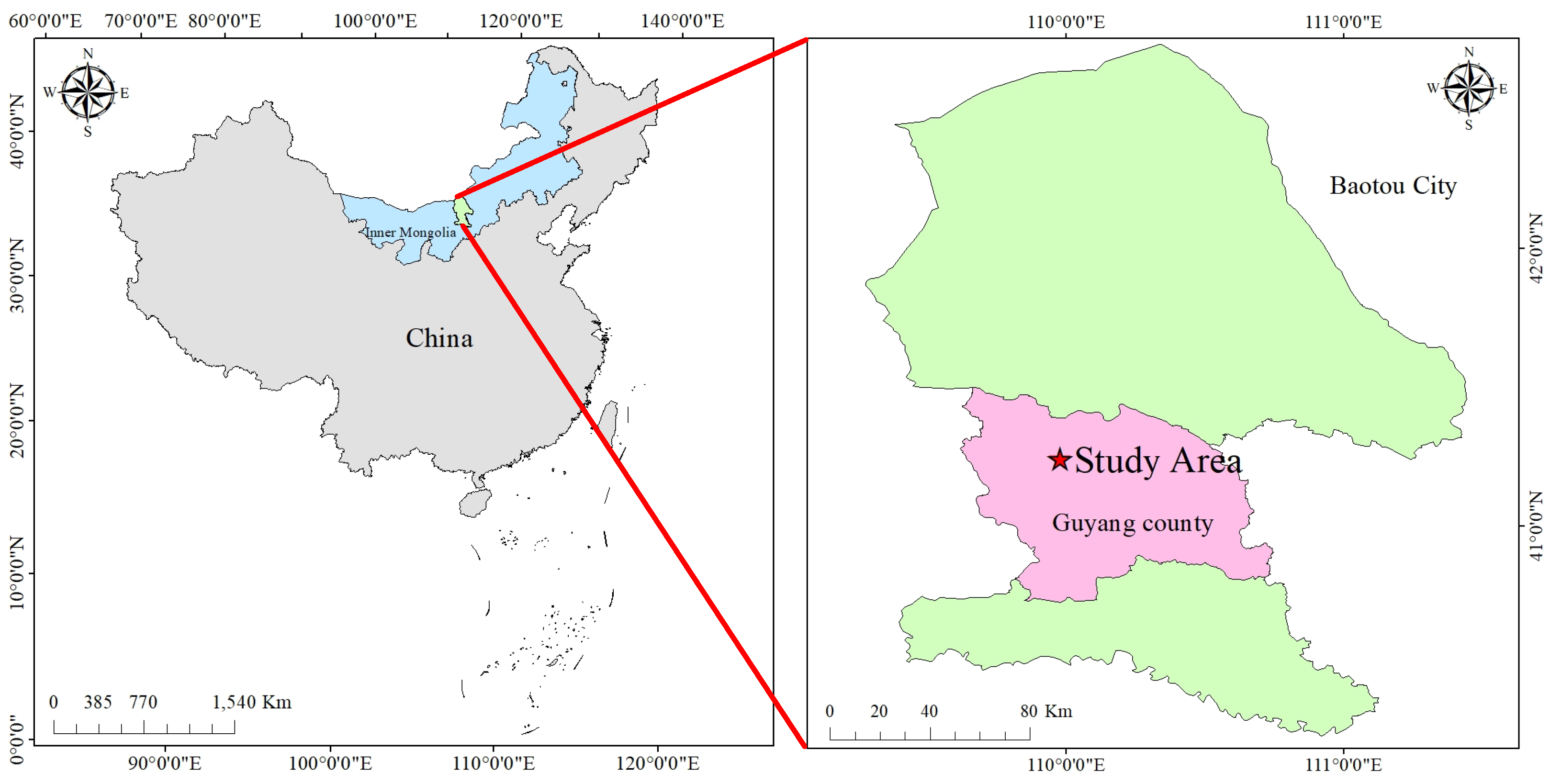
Figure 2.
Diagram of AMM samples and soil samples surrounding AMM roots.
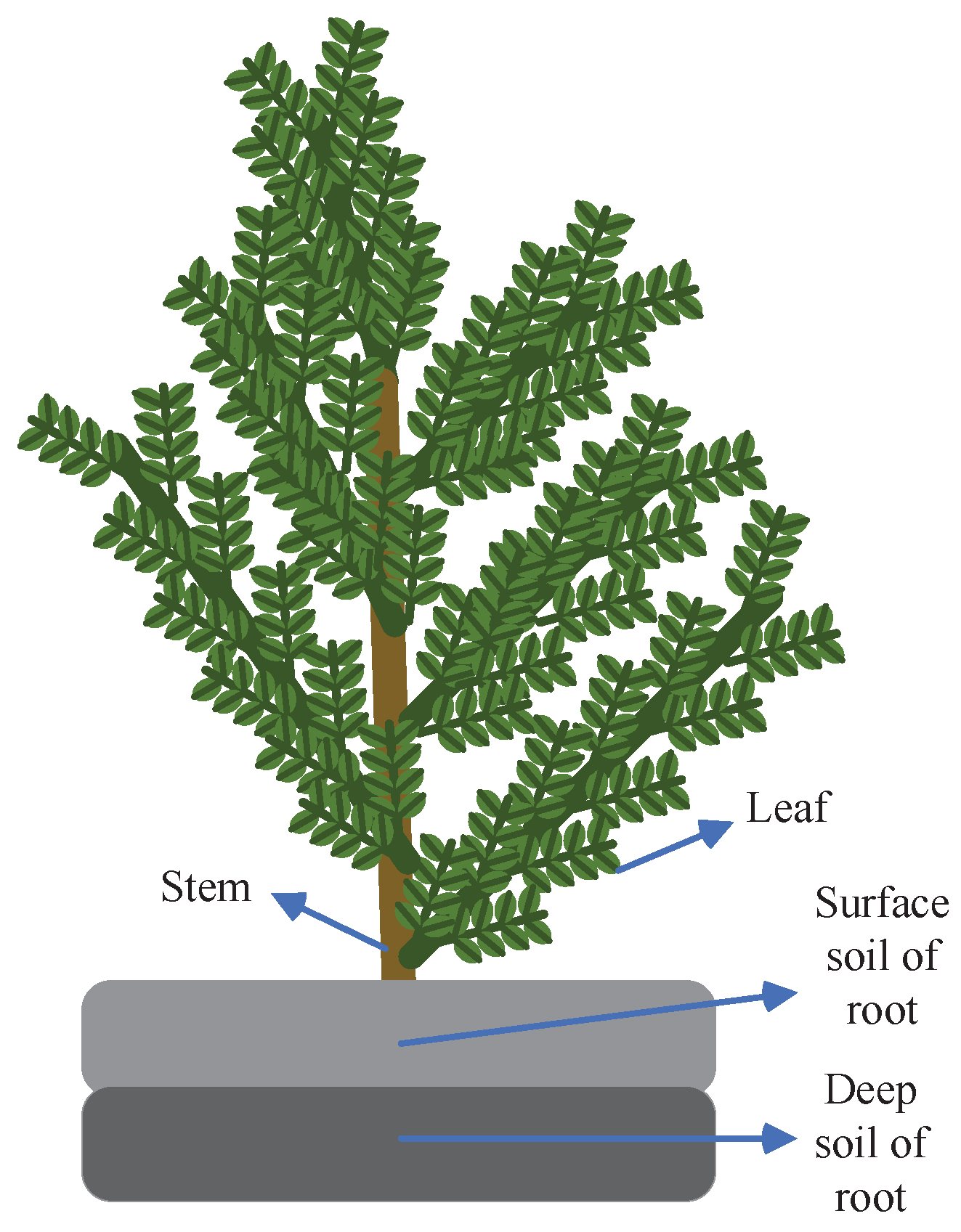
Figure 3.
Scene map of hyperspectral data capture.
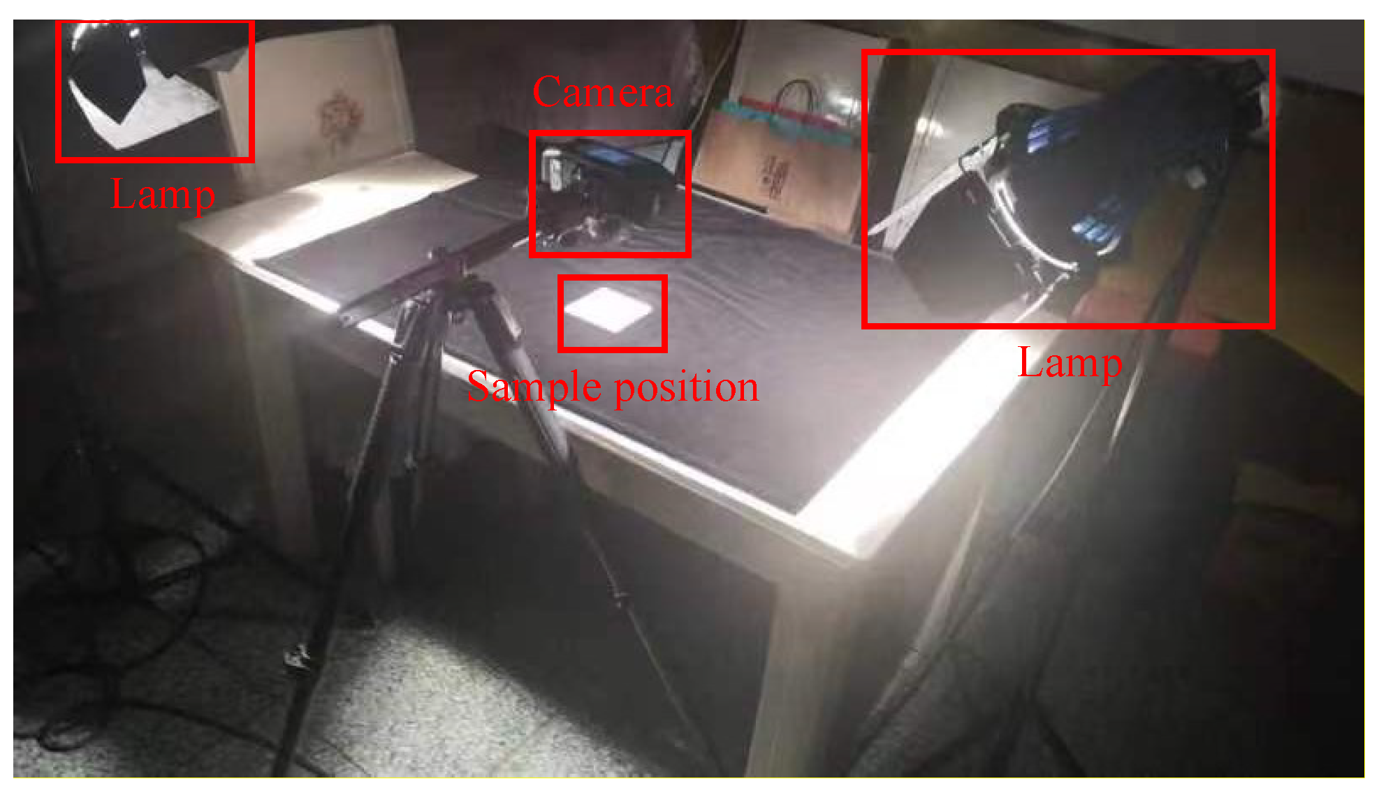
Figure 4.
False color data of hyperspectral data of leaves, stems, surface and deep soil surrounding the roots of AMM.
Figure 4.
False color data of hyperspectral data of leaves, stems, surface and deep soil surrounding the roots of AMM.
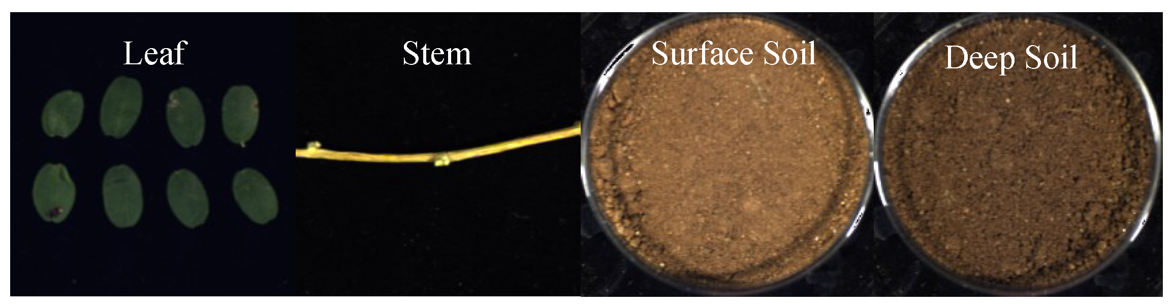
Figure 5.
Diagram of the region of interest.
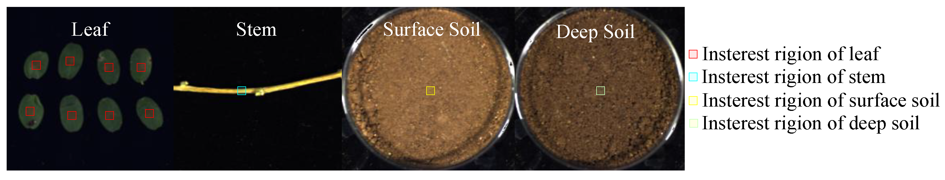
Figure 6.
Spectral curves of the regions of interest.
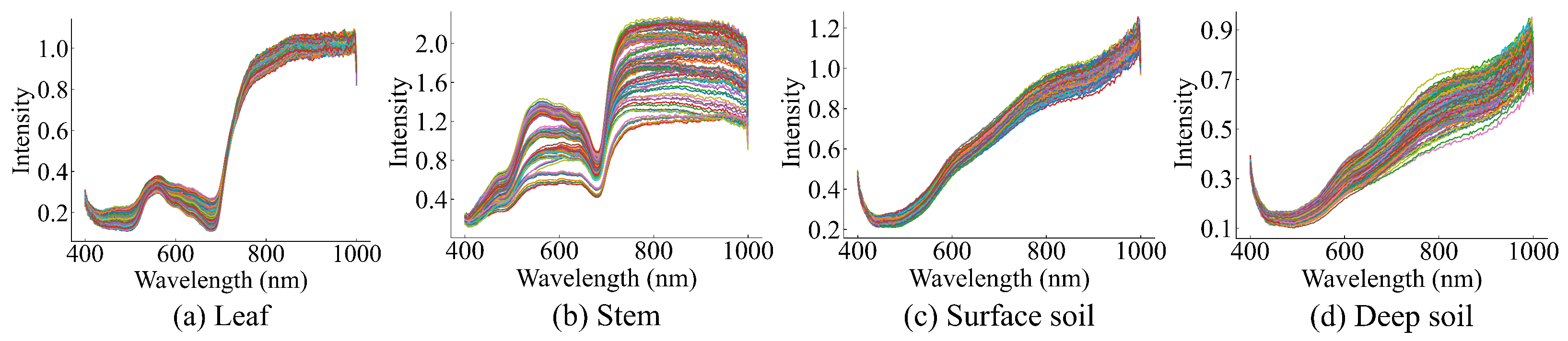
Figure 7.
Histograms of the CC and NC distributions of the leaf samples. (a) Histogram of the CC distribution of the leaf samples. (b) Histogram of the NC distribution of the leaf samples.
Figure 7.
Histograms of the CC and NC distributions of the leaf samples. (a) Histogram of the CC distribution of the leaf samples. (b) Histogram of the NC distribution of the leaf samples.

Figure 8.
Diagram of AM-MHENet.

Figure 9.
Diagram of the improved HybridSN feature extraction module.
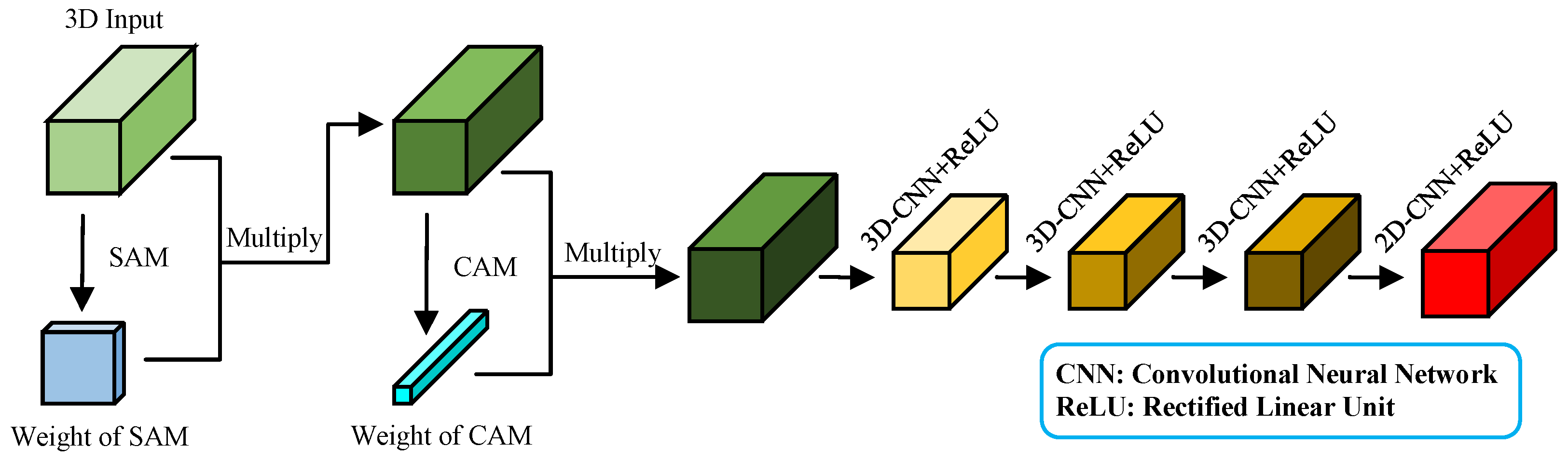
Figure 10.
Diagram of the improved MLP.
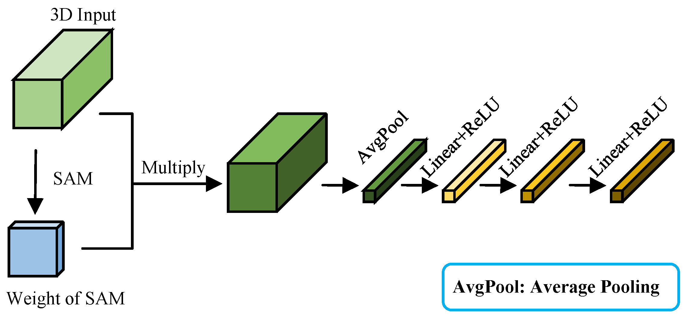
Figure 11.
Flowchart of the hyperspectral estimation algorithm for AMM CC and NC based on multiple hyperspectral feature fusion.
Figure 11.
Flowchart of the hyperspectral estimation algorithm for AMM CC and NC based on multiple hyperspectral feature fusion.
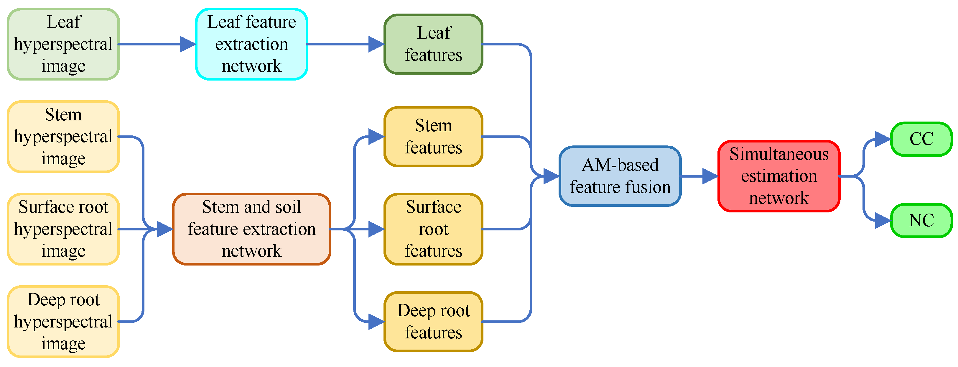
Figure 12.
Diagram of the multivariate hyperspectral feature fusion network module based on AM.
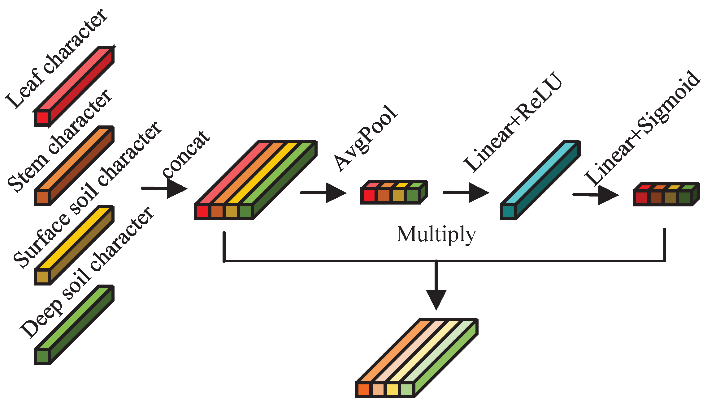
Figure 13.
Diagram of the MLP simultaneous estimation network module.
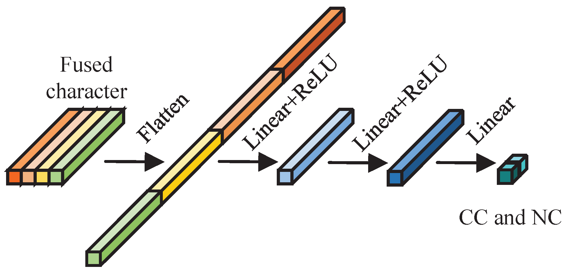
Figure 14.
Scatterplot of the AM-MHENet estimation results.
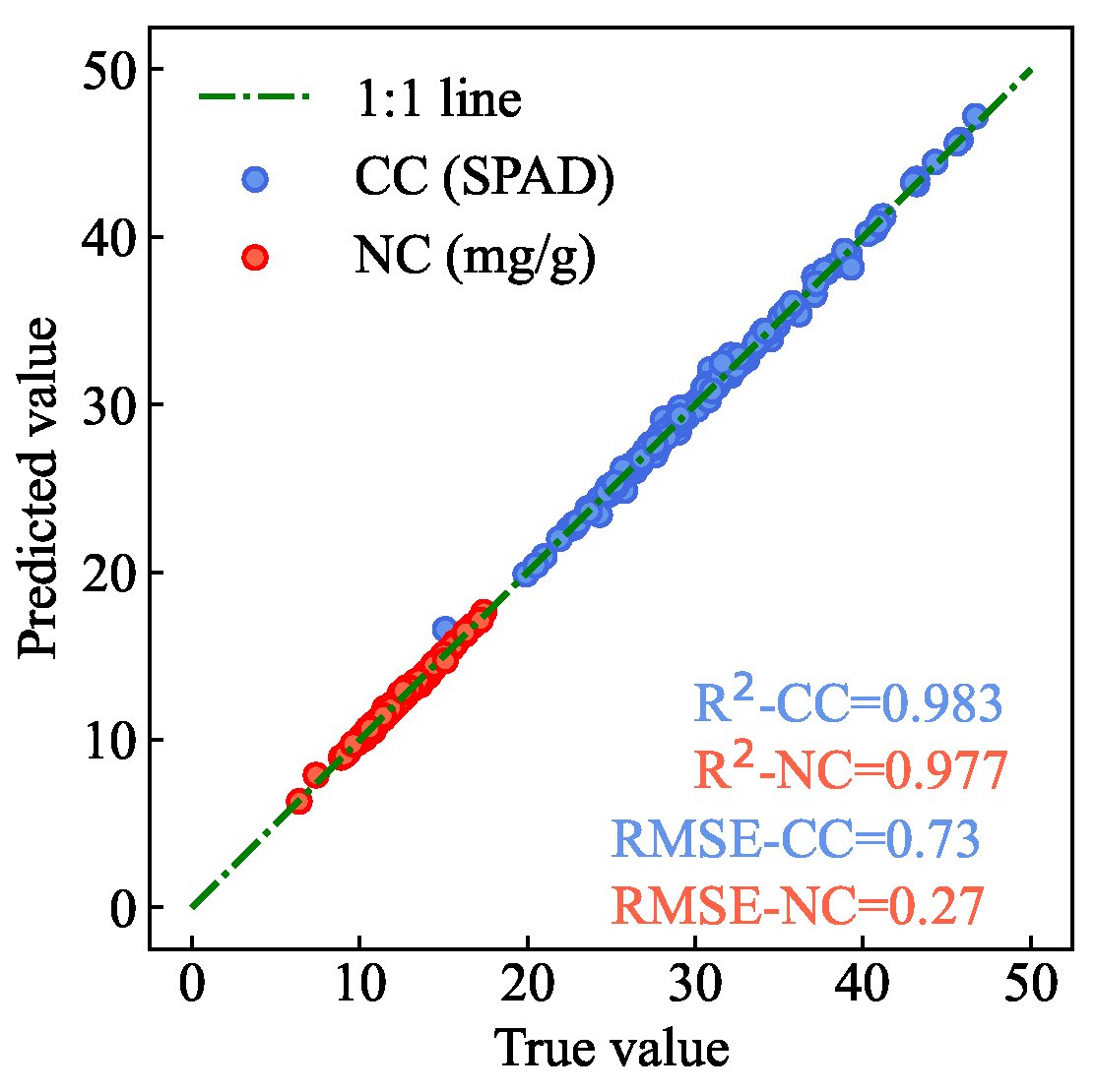
Figure 15.
Histogram comparing the predicted and true CC and NC of AMM leaves.
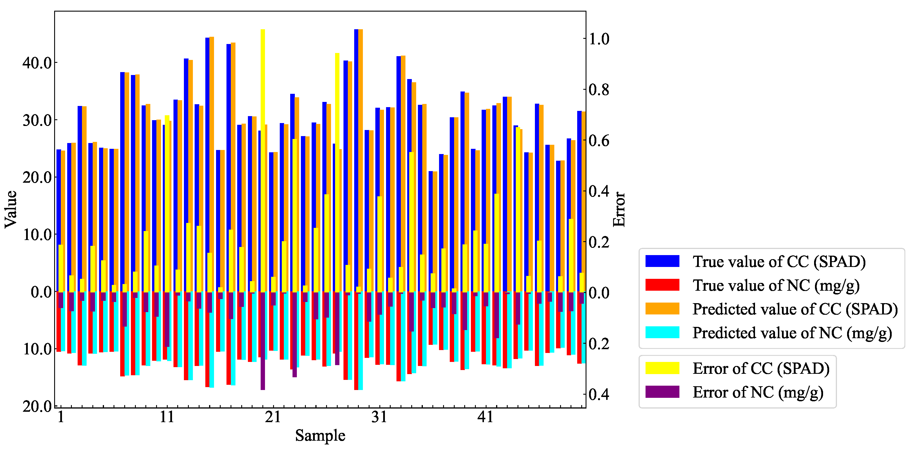
Figure 16.
Heatmap of CAM weight absolute values.
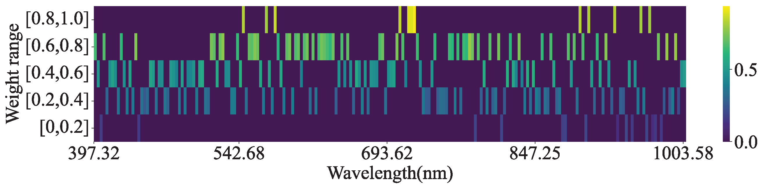
Figure 17.
3D scatter plot of the AM-MHENet estimation results.
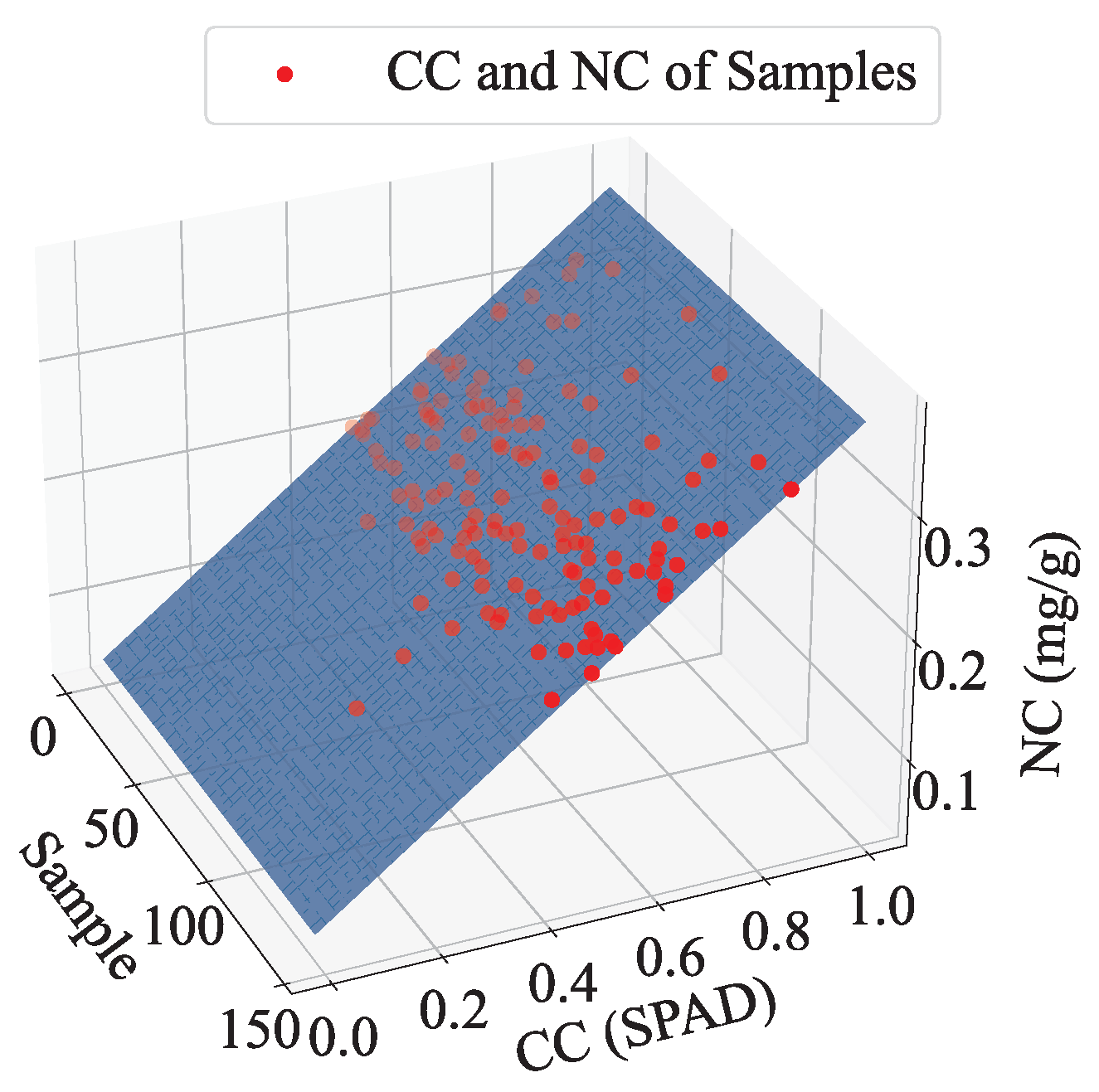
Figure 18.
Distribution map of CC and NC in the partial leaf samples from the test set.
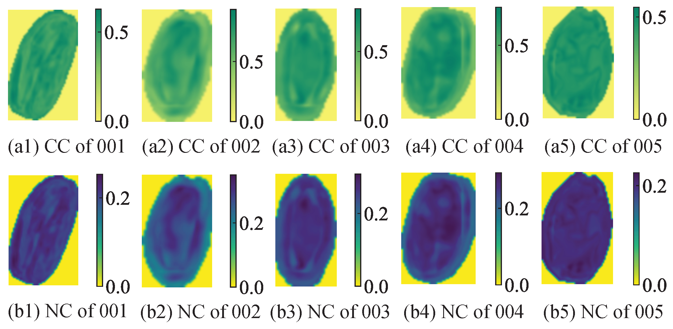
Figure 19.
Predicted and measured values of CC and NC with standard deviations represented as error bars.
Figure 19.
Predicted and measured values of CC and NC with standard deviations represented as error bars.
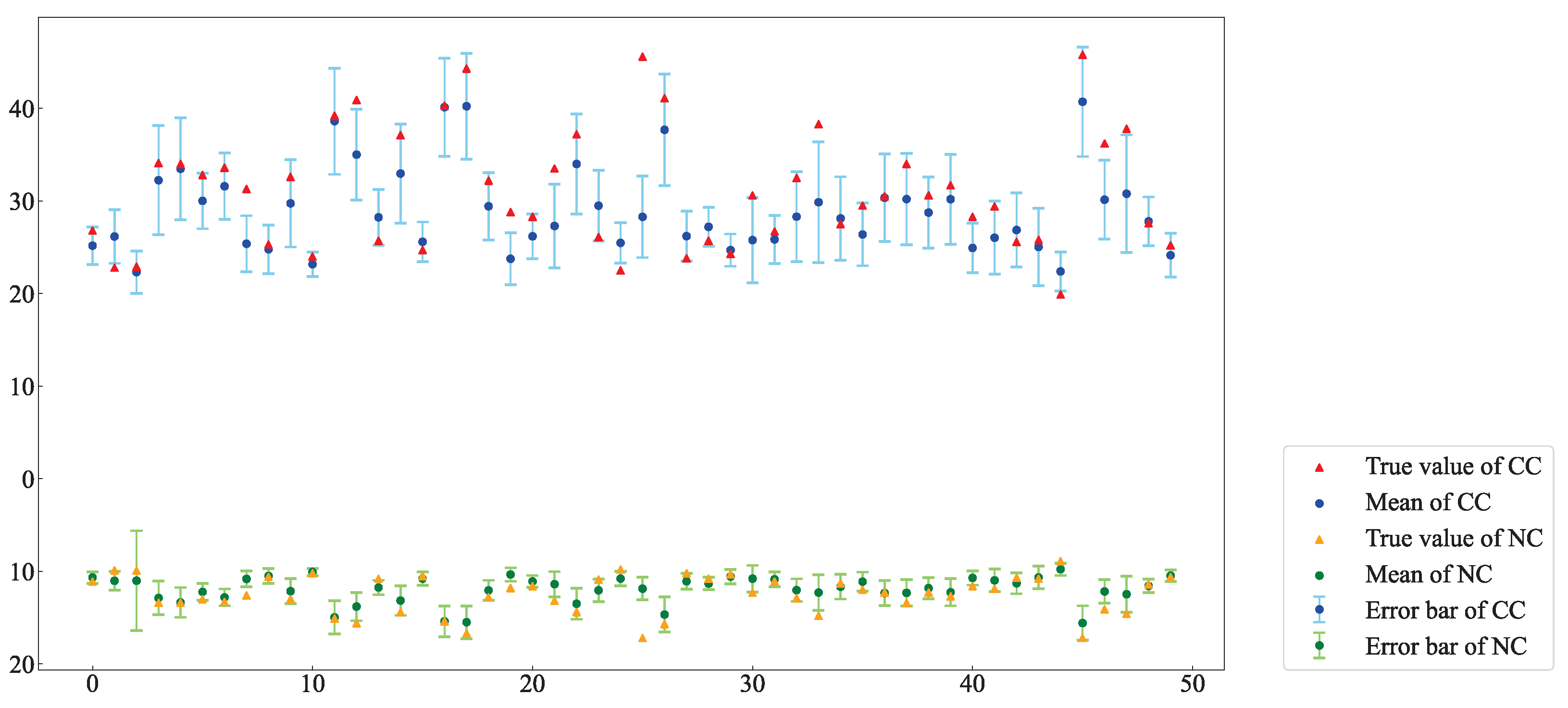
Figure 20.
Comparison of CC and NC estimation results under different feature extraction methods. (a) Inversion results of CC and NC of AMM leaves by the model based on AE for feature extraction. (b) Inversion results of CC and NC of AMM leaves by the model based on PCA for feature extraction. (c) Inversion results of CC and NC of AMM leaves by the model based on GA for feature extraction.
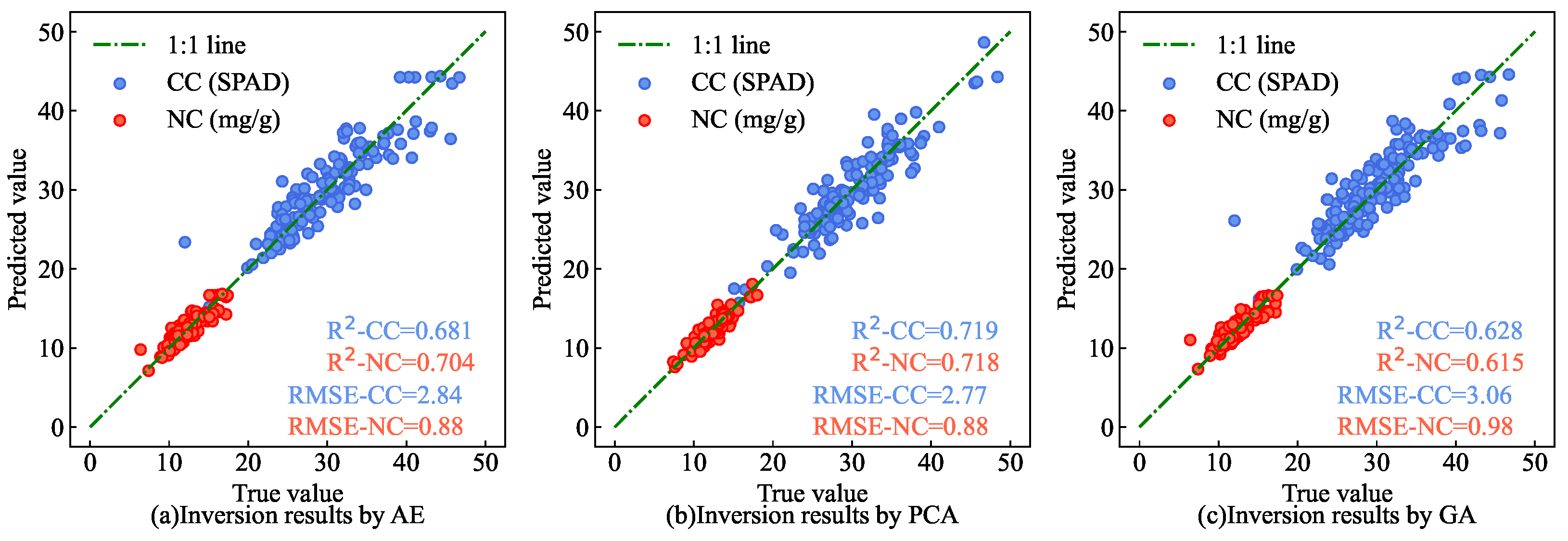
Figure 21.
Comparison of the CC and NC estimation results under the AM ablation experiment. (a) Inversion results of CC and NC of AMM leaves by feature extraction with the feature extraction network module removing AM. (b) Inversion results of CC and NC of AMM leaves by feature extraction with the feature extraction network module removing CAM. (c) Inversion results of CC and NC of AMM leaves by feature extraction with the feature extraction network module removing SAM.
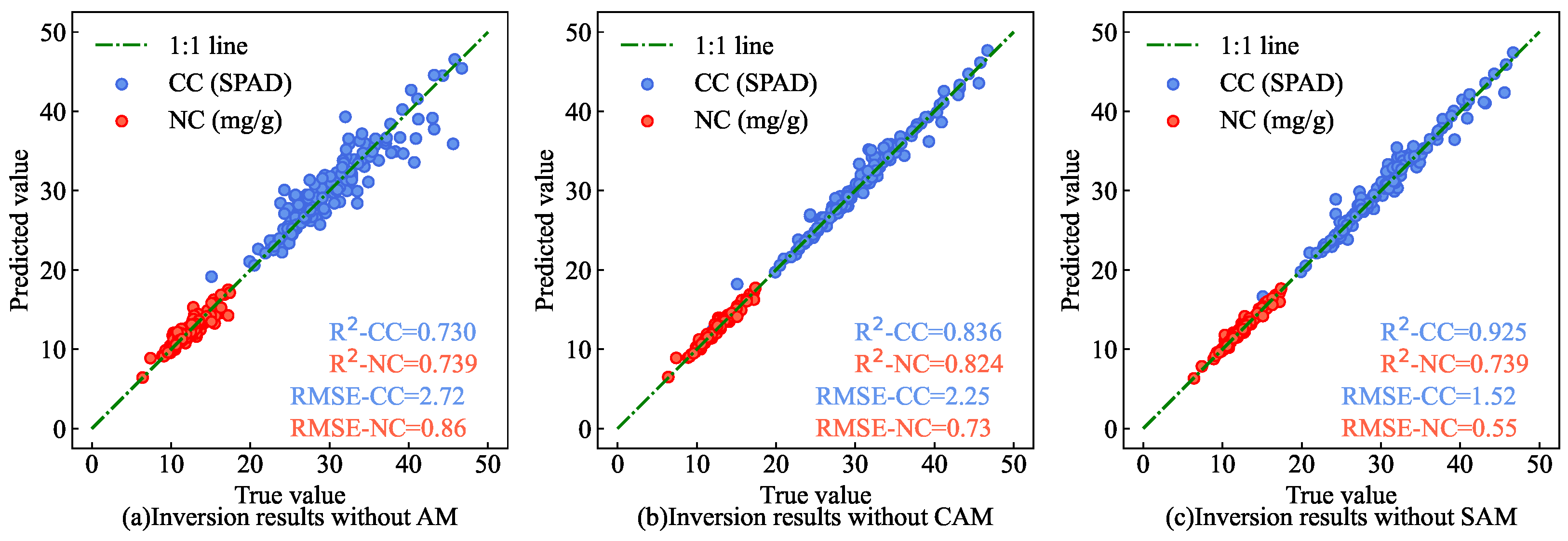
Figure 22.
Comparison of the CC and NC estimation results under different feature fusion methods. (a) Inversion results of CC and NC of AMM leaves by feature fusion network module with feature fusion by ’add’ approach. (b) Inversion results of CC and NC of AMM leaves by feature fusion network module with feature fusion by ’concat’ approach.
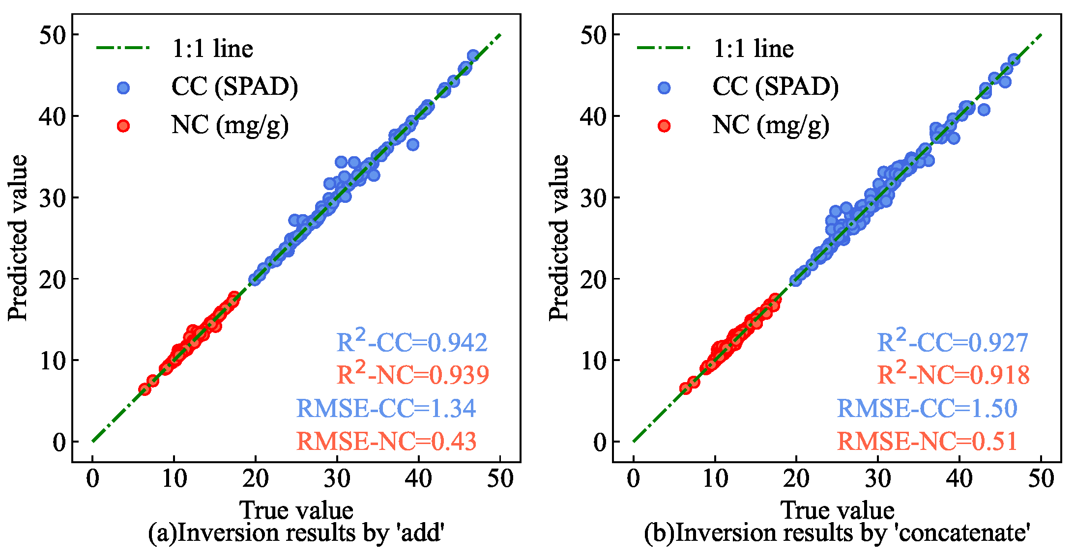
Figure 23.
Single-output estimation results.(a) Inversion results of CC of AMM leaves by the inversion network using CC as model outputs. (b) Inversion results of NC of AMM leaves by the inversion network using NC as model outputs.
Figure 23.
Single-output estimation results.(a) Inversion results of CC of AMM leaves by the inversion network using CC as model outputs. (b) Inversion results of NC of AMM leaves by the inversion network using NC as model outputs.
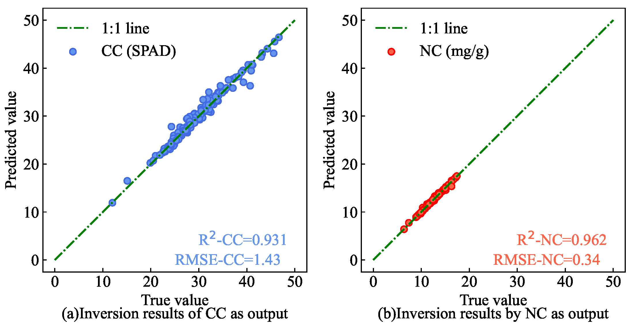
Figure 24.
Comparison of the CC and NC estimation results under the ablation experiment with different input combinations. (a) Inversion results of CC and NC of AMM leaves by the inversion network using only AMM leaf as model inputs. (b) Inversion results of CC and NC of AMM leaves by the inversion network using only AMM leaf and soil as model inputs. (c) Inversion results of CC and NC of AMM leaves by the inversion network using only AMM leaf and stem as model inputs.

Figure 25.
Comparison of the CC and NC estimation results under different estimation models. (a) Inversion results of CC and NC of AMM leaves Inversion results of CC and NC of AMM leaves by PLSR inversion model. (b) Inversion results of CC and NC of AMM leaves Inversion results of CC and NC of AMM leaves by SVR inversion model. (c) Inversion results of CC and NC of AMM leaves Inversion results of CC and NC of AMM leaves by RFR inversion model.
Disclaimer/Publisher’s Note: The statements, opinions and data contained in all publications are solely those of the individual author(s) and contributor(s) and not of MDPI and/or the editor(s). MDPI and/or the editor(s) disclaim responsibility for any injury to people or property resulting from any ideas, methods, instructions or products referred to in the content. |
© 2024 by the authors. Licensee MDPI, Basel, Switzerland. This article is an open access article distributed under the terms and conditions of the Creative Commons Attribution (CC BY) license (http://creativecommons.org/licenses/by/4.0/).
Copyright: This open access article is published under a Creative Commons CC BY 4.0 license, which permit the free download, distribution, and reuse, provided that the author and preprint are cited in any reuse.


