
Submitted:
12 September 2024
Posted:
13 September 2024
You are already at the latest version
Abstract
High mountain rainforests are vital in the global energy and carbon cycle. Understanding the exchange of energy and carbon plays an important role to reflect responses to climate change. In this study, an eddy-covariance (EC) measurement system installed in the high Andean Mountains of South Ecuador was used. As EC measurements are affected by heterogeneous topography and vegetation height, the main objective was to estimate the effect of the sloped terrain and the forest on the turbulent energy and carbon fluxes considering the energy balance closure (EBC) and the heat storage. The results showed that the performance of the EBC was generally good and estimated to be 79.5%. This could be improved when the heat storage effect was considered. Based on the variability of the residuals in the diel modifications in the imbalances were highlighted. Particularly, during daytime residuals were largest (56.9 W/m² on average) with a clear overestimation. At nighttime mean imbalances were rather weak (6.5 W/m²) and mostly positive, while strongest underestimations developed in the transition period to morning hours (down to -100 W/m²). With respect to the Monin-Obukhov stability parameter ((z-d)/L) and the friction velocity (u*) it was revealed that largest overestimations evolved in weak unstable and very stable conditions associated with large u* values. In contrast, underestimation was related to very unstable conditions. The estimated carbon fluxes were independently modelled with a non-linear regression using a light-response relationship and reached a good performance (R²=0.52). All fluxes were additionally examined in the annual course to estimate whether both, energy and carbon fluxes, resembled the microclimatological conditions of the study site. This unique study demonstrated that EC measurements provide valuable insights into land surface -atmosphere interactions and contribute to our understanding of energy and carbon exchanges. Moreover, the flux data provide an important basis to validate coupled atmosphere ecosystem models.
Keywords:
energy balance closure
; heat storage
; carbon fluxes
; eddy covariance
; Andes Mountains
1. Introduction
Tropical forests play a vital role in the global carbon cycle and serve as substantial carbon sinks [1,2,3]. Through their dynamic exchanges of energy, water, and carbon, they shape climate patterns not only regionally but also on a global scale [1,2,3,4]. However, ongoing climate change significantly impacts these land surface-atmosphere exchange processes. Rising temperatures increase the evaporative demand, which feeds back to photosynthetic activities, as indicated by net ecosystem exchange (NEE) [5,6]. Previous research by [1,7,8] has focused on the carbon annual budgets of tropical rainforests. While these studies provide valuable insights into carbon fluxes, they did not specifically address the complexities introduced by heterogeneous terrain. Their findings emphasize the need for dedicated studies that consider the influence of topography on ecosystem carbon dynamics. The tropical mountain rain forest in the Andes Mountains of southern Ecuador represents a unique and biodiverse ecosystem that has received comparatively little attention regarding exchange processes at the ecosystem – atmosphere interface, although they are critical for the global carbon storage [9]. As described by previous studies the area is highly endangered by deforestation [10,11] as well as climate change [12] which impact the exchange of energy, water and carbon. Thus, knowledge on land surface- atmosphere interactions encompassing NEE and the surface energy balance (SEB) play an important role to understand modifications due to global changes.
A commonly used and worldwide accepted approach to directly observe atmospheric carbon and water fluxes is the eddy covariance (EC) measurement technique [13,14]. EC is based on the high-frequency (10-20Hz) measurements of the vertical wind speed and CO2 / H2O concentrations above plant canopies (turbulent eddy flux) coupled to measurements of CO2 storage below the measurement point using slow response infrared gas analyzers [14]. Applying this technique requires extensive quality checks to ensure the accuracy of the measurements across different surfaces [15]. At the same time, certain conditions such as homogeneous and flat surfaces facilitates the estimation and quantification of the fluxes [13,16]. In order to guarantee the quality of the data, quality assessment and control is mandatory especially in non-ideal environments such as the mountainous landscape of the Andes. One of the primary challenges associated with EC measurements in complex terrains is the occurrence of stable atmospheric conditions, particularly at night during nocturnal boundary layer (NBL) development. The atmosphere can evolve a thermally stable stratification, which strongly affects turbulent exchanges and a modified turbulent kinetic energy (TKE) [17,18]. This may lead to an accumulation of CO2 near the surface causing an underestimation of nighttime ecosystem respiration as a result of a reduced or intermittent TKE [13,14]. In contrast, a decoupling between the NBL and the air masses aloft can induce an overestimation of particle quantities due to a break-up of the NBL. The result is an energy imbalance reported by various studies [19,20,21]. Further, in tropical rainforests, the often-dense canopy structure significantly limits the amount of solar radiation that reaches the forest surface. Consequences of the reduction in ground-level radiation can be a modified SEB reflected in the energy balance closure (EBC), which is a critical validation step for EC measurements. As shown by [22,23] an EBC in an acceptable range is also relevant in the interpretation of the atmospheric H2O and CO2 fluxes. However, uncertainties in association to EBC frequently occurs. [20,23] showed that in complex areas residuals can reach up to 35%. Additionally, the footprint area of the fluxes can become more variable, due to the heterogeneous surface characteristics inducing upslope and downslope flows in the diurnal cycle, which is frequently evolving [24], especially in our study site, [13,14]. Further, forest ecosystems can impose a storage effect between the level of flux measurements above canopy and the surface due to the understory. [25,26] investigated the heat storage effect in a mid-latitude forest ecosystems and its effect on the EBC. They found a total heat storage varying between -35 and +45 W/m². This heat storage can create biases in land surface modelling. [27] showed that biases in sensible and latent fluxes are related to the lack of heat storage in vegetation biomass using the Community Land Model version 5. [28] also reported on the improvement of the modelling results under the consideration of the heat storage effect of forest ecosystems. Thus, estimation of uncertainties in EC measurements is crucial and needs a careful consideration as they are also relevant for coupled atmosphere ecosystem modelling.
However, several studies over the past decade have also successfully utilized EC measurements in complex terrain or non-ideal condition [23,29,30]. For the European alpine region [31] have employed these techniques to manage turbulent advection and account for sloping terrain effects. While these corrections and approaches can help to reduce uncertainties in the measurements, the studies also highlight that achieving accurate and closed energy balance in complex terrain remains a significant challenge for the EC method. [3,32,33,34] amongst others have specifically tackled the challenges posed by complex terrain in tropical ecosystems. [32,34] observed dependence of u* on the daytime EBC and demonstrated that the EBC was highly related on the thermodynamic stability of the lower atmosphere. In dry tropical forests, [31] have successfully used EC measurements In which based on the TKE the authors used dimensionless turbulence filters and corrected radiation measurements to address these challenges.
In order to get a better understanding of the energy and carbon exchange in tropical mountain rainforest ecosystems and the response to recent and future climate changes reflected in coupled atmosphere ecosystem modelling observations are highly needed. Therefore, the main objective of this study is the analyses of the influence of the terrain complexity and vegetation height on the turbulent exchange of momentum, energy and carbon using EC measurements above a tropical forest canopy. The aims are to (i) analyze the wind field to assess the advection and turbulent activities, (ii) examine the EBC to estimate the quality of the EC measurements, quantify the imbalance of the heat fluxes and the storage effect of the forest vegetation and (iii) explore on the quality of the carbon fluxes by analyzing NEE in the diurnal and annual cycle. The accuracy of the measured energy and carbon fluxes is highly important for a subsequent partitioning of NEE
2. Data and Methods
2.1. Study Site
The study site is nestled within the tropical montane forest of the Reserva Biológica San Francisco (RBSF), situated on a north-facing slope within the Cordillera Real of the Andes in South Ecuador, the forest type has been described as evergreen lower montane forest [35]. From a permanent one-ha forest plot directly adjacent to the eddy-covariance station we have the following information on forest structure and tree species composition: The species-rich forest contains 1030 stems (with dbh >= 10 cm) of 88 different tree species per hectare. Trees reach maximum heights of 20 m and diameters of 75 cm. Most common tree species are Alzatea verticillata (Alzateaceae, 121 stems), Hieronyma fendleri (Phyllanthaceae, 104), Graffenrieda emarginata (Melastomataceae, 73), and the most common tree families are Lauraceae (227 stems), Melastomataceae (125), and Alzateaceae (121). Aboveground tree biomass was estimated to be 175.8 Mg ha-1 using the formula of [36]. The climate is dominated by the persistent easterly trade winds [37]. Throughout the study period from 2020 to 2022, the mean annual temperature was recorded at 15.4°C, with an average annual precipitation of 1854 mm.
2.2. Instrumentation
The eddy flux tower is located at 3.9737°S / 79.0751°W at an altitude of 1984 asl (Figure 1). It is equipped with an open-path infrared gas analyzer and 3-D sonic anemometer (IRGASON, Campbell Sci.) to measure H2O / CO2 fluxes at a frequency of 10Hz. The EC system is installed in a height level of 23m, which is approximately 1.5 times the mean canopy height. Additional meteorological sensors are installed over the canopy to measure the radiation components short-wave incoming (SWin), short-wave outgoing (SWout), long-wave incoming (LWin) and long-wave outgoing (LWout) using a net radiometer (NR01, Hukseflux), besides photosynthetic active radiation (PAR) (SKP215, Skye Instruments) air temperature (Ta) and relative humidity (RH, VAISALA HMP115). Precipitation is measured using a tipping bucket rain gauge. To obtain soil conditions a TDR soil water sensor (CS655, Campbell Scientific) in a depth of 20cm is installed, which measures soil moisture content (SWC) as well as soil temperature (Ts). A self-calibrating heat flux plate (HFP01-SC, Hukseflux) is used to measure the soil heat flux (G). All variables were sampled and averaged to half-hourly intervals using the CR6 data logger (Campbell Scientific). To estimate the temperature and humidity profile below the canopy Hobologgers (MX2301A) were installed at 1m, 7m, 12.5m, and 16m. The time period considered for the study is January 2020 to December 2022. The PAR sensor is available for the time period March – December 2022 and Ta / RH profiles from October – December 2022.
2.3. EC Raw Data Processing
The 10Hz raw data are processed using EddyPro version 7.0.9 (https://www.licor.com/env/products/eddy_covariance/eddypro). In order to reduce uncertainties in the data and guarantee data quality various techniques have been us. Half-hourly averaged values of the biometeorological variables which are measured with a lower time resolution (30 min) than EC were used as an additional input for the EddyPro Software package to get better estimates of the fluxes. These variables are measured with a lower time resolution than EC. The full output of EddyPro contains time-synchronized fluxes. Random uncertainties arising out of the flux-sampling error are computed following [38]. Other techniques such as despiking [39] and block averaged detrending have been applied to the data as well. Low-pass corrections [40] are applied to compensate for the loss of fluxes towards the low and high-frequency ranges of the cross-spectrum, respectively. Such losses can arise out of inefficient filtering and/or time averaging [41]. In addition, coordinate rotation was performed using the planar-fit method with wind sector divided into 30° [42]. The footprint of the EC tower was calculated according to [43].
2.4. Processing the Half Hourly Data
The initial processing of the half-hourly interval data produced by EddyPro was subjected to rigorous quality control procedures to ensure the accuracy and reliability of the dataset. The following steps outline the methodology used for data filtering and cleaning. The primary step in the data quality control process involved spike detection using the Median Absolute Deviation (MAD) method [15]. This robust statistical technique identifies outliers by calculating the median of the absolute deviations from the dataset's median, providing a measure resistant to extreme values. Subsequent to spike detection, a filtering criterion based on the mean ± 2 standard deviations (SD) was employed [15]. To further improve the quality of our data, we carefully considered the impact of precipitation events, which significantly influence the fluxes at our study site. Specifically, we discarded data collected during precipitation events, as well as data from periods immediately preceding and following these events. By examining the time series plots and other graphical representations, we ensured that any remaining outliers or irregular patterns were addressed. Following the visual inspection, any data points identified as erroneous or inconsistent were manually removed from the dataset [19].
2.4.1. Energy Flux Data
We carefully separated the data based on nighttime, transition times and daytime periods. We tested the impact of turbulences on energy fluxes by applying u* filtering as suggested by [32]. The authors applied this filter for nighttime data where values above a threshold of u* > 0.4 were discarded. This process removed the unrealistic high positive energy flux values, which occur due to large eddies evolving in down-valley winds. For the daytime period when strong mixing lead to high turbulent periods of 0.5 > u*> 1, negative or close to zero values were discarded observed during peak noon period usually considered with high turbulence, except the values impacted due to precipitation event. Similarly, during transition periods where u* is fluctuating between stable and unstable conditions, such ambiguous data periods were mostly discarded. Implementing these measures, we aimed to refine our dataset and improve the reliability of the EBC analysis.
2.4.2. NEE Data Filtering
Standard procedure was applied, including u* filtering to exclude low-frequency data obtained during stable conditions. The u* threshold was determined using the moving point technique [44], with a u* threshold of 0.23 m/s. Nighttime negative values of NEE was also discarded. Additionally, we discarded data where the Monin-Obukhov stability parameter ((z-d)/L) exceeded 0.2. The theory suggests a dimensionless parameter which characterizes unstable condition ((z-d)/L) < 0), stable conditions ((z-d)/L) >0) and neutral conditions ((z-d)/L) =0) [45,46], where z is measurement height and d is displacement height.
2.5.3. Correction for Global Radiation:
Since the NR01 is installed over a sloped surface above canopy and thus, not mounted perpendicular corrections must be applied to shortwave incoming radiation (SWin) as the measurements are dependent on the slope and aspect of the surface [31,41]. The model and methodologies presented by [47,48] were thus used to correct the measurements at the sloping site. The procedure requires calculations of the solar zenith angle (θz) and the angle between the horizontal to the inclined surface and the direction of the sun (ψ2; all angles are expressed in radians). We calculated the corrections using an additional EC system in the study site installed over a plane surface[49] . Using measurements of SWin radiation at the reference site, the incoming solar radiation for an inclined plane (SWψ) can be calculated by applying the following equation, as described by [48]:
where, kt values were calculated using the ratio of SW and estimates of the extra-terrestrial radiation and A values were calculated using SWin and SWout measurements from the net radiometers, the solar zenith angle (θz) and the angle between the horizontal to the inclined surface and the direction of the sun using NOAA's Solar Calculator based on astronomical algorithms [50].
2.6. Heat and Moisture Changes in Canopy Air
At 4 different height levels above ground, i.e. level 1 = 1m, level 2 = 7m, level 3 = 12.5m, and level 4 = 19m, we installed low-budget temperature / relative humidity sensors to estimate the vertical heat and moisture development in the diurnal cycle. The changes along the profile in the understory air are to test the storage effect of the forest ecosystem, which contributes to the overall estimation of the quality of the fluxes. The data were normalized based on the measurements above canopy obtained from the EC system. This ensures a consistent comparison of heat and moisture variations within the canopy air. The normalized values defined as:
With Ta and RH as temperature and relative humidity, ref as the reference value, i as the value at the respective height level (1, 6, 12.5, 19m).
To quantify the heat and moisture storage integrated between 0m agl. and canopy height (zc = 25m), we used the theoretical definition also described in [26]. It is defined as:
with SH and SLE as storage (S) of sensible heat (H) and latent heat (LE), ρa and ρv as air density for dry and wet air, cp the specific heat capacity, L latent heat of vaporization, t is time and zi are the respective height levels (1, 6, 12.5, 19 and 25m). Written as finite differences and summarized over the time increment Дt = 30 minutes result in:
3. Results
3.1. Wind Field
Mountainous regions are highly dominated by slope winds developed in the diurnal cycle and affecting the planetary boundary layer (PBL). Because of the location of the EC system, we start our analyses by looking particularly at this mechanism and its impact on the turbulent fluxes. Figure 2 shows the wind field (speed and direction), u* and the Monin-Obukhov stability parameter ((z-d)/L).
Generally, a clear diurnal cycle can be observed for each variable illustrated, which points to the occurrence of changing wind fields in the diel. Wind direction is rapidly changing especially in the transition between daytime and nighttime hours. While from 9:00 – 17:00 the northeastern direction (35 – 65 degree) dominates representing up-valley flows, it is changed to a southeastern direction (155 – 175 degree) from 18:00 – 7:00 indicating down-valley flows. The slope valley winds tend to be stronger during late morning and afternoon hours as the irradiance creates the stronger gradients. This is reflected in the wind speed and u* as well. They feature the highest (lowest) values from 9:00 - 17:00 (7:00 - 8:00) associated with the strongest (weakest) variability. During daytime wind speed ranges from 4 - 6 m/s while during night time it declines down to 2.5 m/s. The maximum wind speed of 9 m/s is observed at 12:00 with a corresponding strong u* of 2.10 m/s creating strong turbulent mixing. The situation is changed during nighttime, when calm conditions predominate and mixing is weakened as indicated by u* varying between 0.1 - 0.75 m/s. Further, the variability of both, wind speed and u*, is distinctly reduced during nighttime hours.
The Monin-Obukhov stability parameter ((z-d)/L), confirms the variations in the turbulence activities from the surface to the canopy in the diurnal cycle. The lower atmosphere is mostly turbulent during the late morning period (08:00- 09:00) as indicated by the strongest negative values ranging from -0.2 to 0.2. This is the hour of day, when wind direction is changing and speed is increasing, resulting in the development of the PBL neutral and unstable conditions (values ≤ 0) during daytime. The atmospheric stratification is modified to stable conditions (values > 0) at nighttime with mostly positive values. Fluctuations towards negative values can also be observed due to down valley winds which induces turbulent kinetic energy (TKE) within the NBL [17,18].
3.2. Vertical Heat and Moisture Effects
As well known, forest ecosystems evolve a storage effect due to differences in the vertical energy transportation within the understory and at the canopy [51,52]. Storage effects within the canopy related to air temperature and relative humidity involves the retention and exchange of heat and moisture within the canopy and surface layers, which feedback to the ecosystem's energy balance. In terms of the rate of CO2 fluxes, it is determined by the difference in the instantaneous profiles of concentrations at the beginning and end of the 30-minute EC averaging period, divided by the averaging period itself [51,53]. During nighttime, when the atmosphere is stable stratified and turbulence is weak, the storage effect becomes important as it may exceed the CO2 fluxes. For this, as mentioned above we installed 4 low-budget sensors at different height levels within the canopy to estimate a storage capacity concerning air temperature and relative humidity profiles.
Figure 3 illustrates the storage capacity for heat and moisture calculated based on equation 2. Normalized values > 1 (< 1) indicate higher (lower) values than above the canopy at EC measurement level (zc), while 1 represents equal values. This means, unstable, stable and neutral stratifications, respectively, can be derived. Generally, the strongest temperature deviations are developed during daytime while the nighttime hours oscillate around 1 Figure 3 (a). With exception of level 1 warmer Ta occur during daytime, particularly for level 3 and 4. Here, higher values than above the canopy between 15% (1.15) and 25% (1.25) are, rapidly develop in the morning hours and remain over the day. The lowest level (1 m agl) in contrast shows below-reference values down to 10% (0.9), which indicates cooling effects near the ground. Height level 2 fluctuates around 1 throughout the day with highest values in the afternoon (13:00 – 16:00) and lowest values around early evening (17:00 – 18:00). RH, illustrates the opposite behavior with highest deviations from reference in 1m (> 60%) around noon Figure 3 (b), which represents an accumulation of moisture near ground. Level 3 and 4 on the other hand are close to 1 and below the reference, which points to drier conditions than above the canopy.
3.3. Energy Balance Closure
One of the greatest challenges of EC measurements, particularly in sloped and heterogeneous terrain, is the EBC as described by various authors [24,34,54]. However, it offers a possibility to validate EC measurements by the sum of LE and H against the difference between net radiation (Rn) and ground heat flux (G) through linear regression analysis [14,55]. It is defined as
Rn
= LE + H + G + ε
with ε as residual flux representing the imbalance.
Figure 4a shows the EBC with an explained variance of R² = 0.795, which characterizes a good closure and is in the range of uncertainty in complex terrain [22]. In order to explore on the behavior of the energy fluxes Figure 4 (b) shows the mean diurnal cycle of H and LE, in which also, Rn and the corrected net radiation (Rn*) are examined. As expected, the energy fluxes resemble a strong diurnal cycle with a peak around noon and a decline at night. LE is the strongest contributor to the energy exchange at our site with a mean maximum of 400 W/m², while H reaches 200 W/m². Interestingly, G reveals a lag in its peak phase for both, daytime and nighttime hours.
To reduce uncertainties in the EBC we corrected Rn as described by [23,30,31]. Comparisons between Rn and Rn* illustrate that the corrections applied clearly affect the magnitude of the radiation budget (Figure 4b). While Rn reaches a maximum of 450 W/m² during daytime Rn* exhibited a reduced magnitude (320 W/m²). For nighttime this behavior is changed and Rn features a stronger radiation loss than Rn*. The most significant modifications are occurring in the morning hours as well as during daytime. Although both Rn and Rn* peaked at noon, the latter resembled a more smoothed pattern. Despite these adjustments, the overall improvement in EBC was only marginal as indicated by R² = 0.795 (Rn) in comparison to R² = 0.794 (Rn*). Since the magnitude of Rn* was consistently lower than LE, as well as that the accuracy of the EBC has not been improved significantly, the uncorrected values are used in the ongoing analyses.
Considering the storage effect on heat (SH) and moisture (SLE) exchange the EBC and diurnal cycle of LE and H are additionally included for the time period October 2022 – December 2022 (Figure 4c, d). When the storage is added an improvement of the EBC from R²=0.786 to 0.789 and a root mean square error (RMSE) from 121.37 to 120.37 is achieved (Table 2). Although the effect is only marginal, especially the diurnal cycle reveals important insight into systematic patterns.
Table 3 summarizes the mean and integrated storage effect related to the mean diurnal cycle as well as to daytime, nighttime and transition hours as defined in (Table 1). In total on a daily basis SH and SLE accounts for 4.4 and -5.6 W/m², respectively. When we take a look at the hours of day, it can be observed that H generates an overestimation of heat (SH) of more than 10 W/m², especially from 8:00 - 10:00, with a subsequent decline from noon down to 5.5 W/m², when mixing is strongest. For LE an underestimation occurs as indicated by the negative values of SLE. It reaches its lowest values from 10:00 – 14:00 with around -12 W/m². As an integral value SH and SLE account for 105.2 and -133.7 W/m², respectively, 55% and 40% of which is generated in the transition hours.
3.4. Energy Balance Closure as a Function of Time
As the diurnal cycle of the storage capacity (Figure 3 and Figure 4) revealed variations in heat and moisture on daytime (11:00 - 14:00), nighttime (20:00 – 6:00) and transition (7:00 – 10:00, 15:00 – 19:00) hours, we additionally established the EBC for these time periods. Table 4 summarizes the linear regression coefficients as well as the R² and RMSE.
The results confirm a clear decrease in EBC during the day (R² = 0.545), while in the transition the explained variance increased to R² = 0.666. This is also reflected in the RMSE with 107.29 against 133.32 for daytime and 108.36 for the transition hours.
With respect to ε of the EBC differences between daytime and nighttime imbalances can be observed for both, the entire time period and the sub-period related to the storage effect (Figure 5, Table 3). Basically, during nighttime on average imbalances are close to zero. As the morning hours approach associated with global radiation (Rg) an underestimation of approximately 50 W/m² on average occurs. This is rapidly modified to an overestimation in the late morning hours of around 140 W/m² and peaks prior to the energy flux maxima before declining in the afternoon. Thus, variations in the EBC develop in the diurnal cycle. This is also true for the shorter time period. Comparing ε and ε’ it can be observed that the addition of the storage effect in H and LE (SH and SLE) reduces the imbalances. However, divided into the three time periods, it can be noted that daytime hours contribute the most to the imbalances, which accounts for 64% of the total amount (356.2 W/m²).
3.5. Energy Balance Closure and Its Relation to Thermodynamic Conditions
In order to shed light into the relation of imbalances to thermodynamic conditions and turbulence activities Figure 6 displays (z-d)/L and u* against ε. Since both, the residuals without and with the addition of the storage effect is comparable, the former ε is used in the ongoing analyses. The data are binned into 20 classes. As a result of averaging over each bin, but to highlight the varying signals, the y axis differs between u* and (z-d)/L.
Based on the stability parameter a clear relationship between an underestimation of the energy balance and unstable conditions can be observed as ε reaches values down to -75 W/m². In contrast, weak unstable to neutral conditions are associated with the strongest overestimation up to 75 W/m². During stable stratifications ε is close to zero, but increases towards a strong stable stratified PBL with an additional higher variability. With respect to u* weak values between 0.1 and 0.5 m/s feature small imbalances, while they increase with stronger u* values resulting in large overestimations. Reaching a u* value of more than 1.8 m/s ε decreased sharply down to 50 W/m².
Separated into the three time periods of the day (Table 1) and also visible in Figure 5, variations in the amount of imbalances can be recognized. Figure 7 illustrates that daytime imbalances vary between strongest overestimations (100 W/m²) during weak unstable to neutral conditions (-1 < (z-d)/L < 0.5) and strongest underestimations (-100 W/m²) during weak stable conditions ((z-d)/L > 1). Nighttime in contrast generates a rather small overestimation (5-50 W/m²) of the EBC independent on the stability, while the transition time reveals a clear relationship between the thermodynamic stability and ε. Imbalances as a function of u* reflects a similar behavior pointing to the turbulence activity. During daytime, when strongest mixing occurs (u* > 0.5 m/s), overestimations are largest (up to 250 W/m²), while nighttime hour represent calm conditions with the smallest ε values varying slightly between positive and negative imbalances (-30 – 20 W/m²). In the transition time, when mixing is modified imbalances change from under – to overestimation around -50 – 50 W/m².
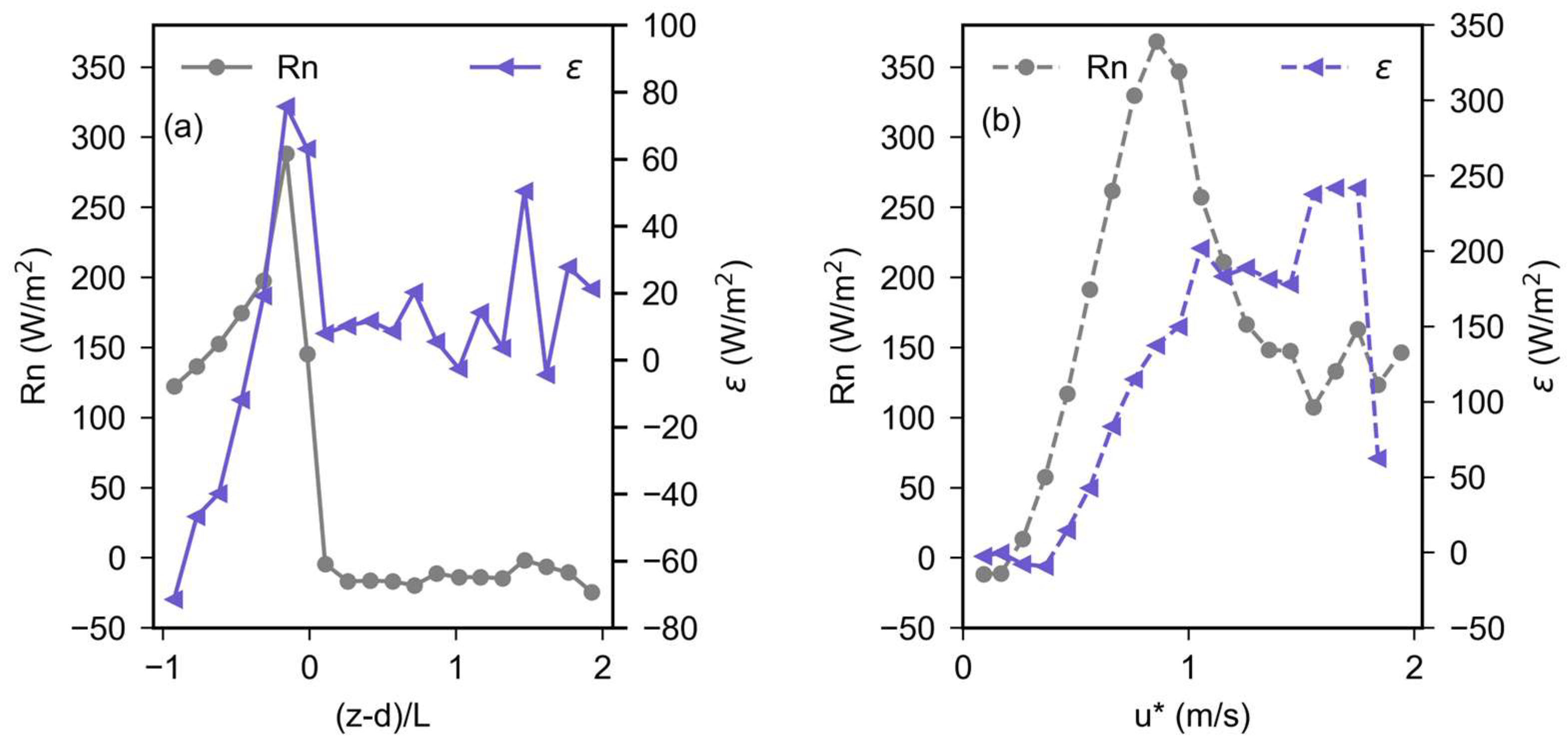
Considering the relationship between ε and Rn as a function of (z-d)/L and u*, it can be observed that strongest overestimations of the energy balance is associated with higher irradiance. This is particularly true for the stability parameter, which reveals the peak phases for weak unstable to neutral conditions. According to u* Rn peaks with 350 W/m² between 0.5 and 1.0 m/s. Interestingly, the strongest imbalances (250 W/m²) occur during lower irradiance of around 100 W/m² representing again the transition hours of the day.
Figure 8.
Binned means of residuals (ε, W/m2) and net radiation (Rn, W/m2) as a function of (a) Monin-Obukhov stability parameter (z-d)/L and (b) friction velocity (u*, m/s).
Figure 8.
Binned means of residuals (ε, W/m2) and net radiation (Rn, W/m2) as a function of (a) Monin-Obukhov stability parameter (z-d)/L and (b) friction velocity (u*, m/s).
3.6. Diurnal Cycles of CO2 Fluxes
Our next step is to examine NEE estimated based on the CO2 flux measurements by the EC system. Because the data encounter similar challenges regarding the data quality as the energy fluxes, careful inspection is required as well. Thus, we explicitly analyze unfiltered NEE and filtered NEE (NEE*) to identify the impact of local wind systems and precipitation events on the carbon fluxes. The diurnal patterns of NEE and NEE* highlight the dynamic nature of CO₂ exchange within the ecosystem. Understanding these patterns is crucial for assessing the carbon balance and the role of the ecosystem.
Figure 9 shows the typical diurnal cycle of NEE and NEE* with positive values during the morning period indicating CO2 respiration and negative values during daytime indicating the absorption of CO2 by the canopy. The maximum absorption of CO₂ is observed between 11:00 and 12:00, with values ranging from NEE = -20 to -22 μmol/m²hour. This peak indicates the highest photosynthetic activity within the canopy during this period. A noticeable shift in NEE during the upwind period is observed between 7:00 and 8:00. During this period, maximum turbulence is seen as indicated in Figure 2d, with NEE shifting from 0.4 to -5 μmol/m²hour. This turbulence likely enhances the mixing and thus, the transport of CO₂ within the canopy. A change in NEE from negative (-3.21 μmol/m²hour) to positive (5 μmol/m²hour) is observed during the downwind period between 17:00 and 18:00 and represents a transition from CO₂ uptake to release as the photosynthetic activity decreases and respiration becomes dominant.
With respect to the correction, difference can be detected in the magnitude of NEE. After filtering NEE reaches lower values of -1.76 μmol/m²hour for the daytime peak and -23 μmol/m²hour for the nighttime hours. The magnitude changes from NEE = -1.4 µmol/m²day to NEE* = -4.28 µmol/m²day, which was also reported by [2]. During the stable conditions underestimation of NEE occur. Discarding this data necessarily minimizes the impact on NEE due to stable conditions [29]. Implementing u* filtering helps to remove periods of insufficient turbulence, thereby reducing the potential bias in nocturnal flux measurements. This leads to a more accurate assessment of ecosystem respiration during nighttime. This filtering is particularly important for avoiding biases in nocturnal flux measurements and improving the overall quality and reliability of the data used in carbon budget analyses [15,44]. We found that the filtered data are better correlated (0.48 for NEE, 0.52 for NEE*) to light availability in terms of Rg and photosynthetic photon flux density (PPFD).
3.7. Light-Response and Carbon Exchange Model
To independently model NEE and explore on the ability to estimate carbon fluxes in such a challenging environment Figure 10 illustrates the non-linear fit of daily NEE as a function of Rg and PPFD, respectively from 8:00 – 16:00 to ensure for a full irradiance. The latter is only available for the time period March – December 2022. The non-linear fits for both, Rg and PPFD resemble typical saturation curves with the strongest CO2 uptake (NEE = -18 µmol/m²day) around 400 W/m² and 80 mmol/m²day, which represents the maximum uptake by the ecosystem under optimal light conditions. Since both models show a R² value of 0.52, a good performance of the carbon exchange model exists. Thus, the variance of NEE can be estimated with independent meteorological quantities, which points to a sufficient quality of the CO2 fluxes.
3.8. Annual Cycle of Microclimatological Conditions, Carbon and Energy Fluxes
Finally, the annual course of the meteorological quantities such as Ta and RH with energy (LE and H) and carbon (NEE) fluxes were analyzed in Figure 11 to examine whether the fluxes resemble the microclimatological conditions. The study site is characterized by a wet period from April till June and drier conditions during September till December [56]. This is clearly reflected in the fluxes as well.
On the annual cycle Ta varies between 12 and 20°C, whereas RH features value between 51 and 99%. Maximum distinction occurs in January for Ta (13.5 - 18°C) and for RH in October (65 - 85%). Months with drier conditions (August - October) have a higher range of Rg (260 - 310 W/m2), while during wet periods (220 - 260 W/m2) occur, most likely due to clouds. The energy (H, LE) and CO2 (NEE) fluxes reflects these micrometeorological conditions. The highest variability can be observed in July and August, where LE reaches up to 165 W/m² and H up to 43 W/m². In contrast, the lowest variability occurs in November (LE) and December (H) with a range of (142 – 137 W/m²) and (53 - 39 W/m²) respectively. The same is true for NEE with the largest range in July (-28.5 – 26.5 μmol/m²day) and the smallest December (-18 – 7.04 μmol/m²day).
4. Discussion
In this study we used energy and carbon fluxes obtained by an EC measurement system above a forest canopy in complex terrain of the tropical Andes Mountains in South Ecuador. The main focus was to investigate of the impact of the terrain as well as the vegetation height on the turbulent exchange of momentum, energy and carbon fluxes essential to quantify uncertainties in the energy balance and the heat storage effect. In such complex areas flux measurements are affected by thermally-driven wind fields in the diurnal cycle. Additionally, the EBC and its residuals were analyzed and reflected in the diurnal cycle with respect to the heat storage generated by the forest ecosystem to quantify the quality of the measurements in this challenging environment.
As expected, the study site influenced by the local wind systems which develop in the diurnal cycle (Figure 2). This means, during daytime hours an upslope flow can be observed, while in the nighttime hours it is reversed to a downslope flow due to net radiation loss. Consequences are varying wind speeds as well as turbulence activities. The latter was confirmed by the Monin-Obukhov stability parameter ((z-d)/L). Here, it was revealed that during nighttime stable stratified atmospheric conditions dominated (values > 0), while during daytime it alternates between neutral (values = 0) and unstable stratified conditions (values < 0). However, especially the transition from nighttime to daytime showed the strongest variability with values down to -0.7. During that time of the day air masses in the downslope flow change their direction to upslope, which creates turbulent activities and a destabilization of the PBL. Advection occurred in the nighttime hours, where downslope flows led to alterations between stable and neutral conditions as indicated by u* reaching up to 1.5 m/s and (z-d)/L fluctuating from 0 to > 0.5, which was also mentioned by [57].
The storage effect was estimated on the basis of heat and moisture profiles within the canopy as well as SH and SLE (Figure 3 and 4). The normalized Ta / RH values in the diurnal cycle revealed strongest deviations from the reference level (zc) at the highest levels in the understory (level 3 and 4) during morning hours (7:00 – 10:00). That means, during transition to daytime and incoming radiation an accumulation of heat and moisture develops, which is not mixed downward. At the same time, strongest turbulence activities above canopy were revealed, which evolves an upward mixing into the atmosphere. The lowest level on the other hand was below zc pointing to an exchange with the soil and stable stratified conditions. From 11:00, when mixing is fully developed as indicated by the maximum of u*, wind speed and (z-d)/L differences between Tanorm and RHnorm are reduced for level 3 and 4, but level 1 showed only weak changes. However, differences between the lower and upper levels highlight the influence of the sloped terrain as well as the vegetation height on the stratification of the air mass column and the storage capacity.
The unstable stratification and energy storage generated high EBC residuals as illustrated in Figure 4 and 5. EBC in total showed a good performance at the study site (R² = 0.795) also described by [20] for tropical rainforest ecosystems in complex terrain. For instance, [31] studied a dry forest ecosystem with complex terrain and found EBC values that varied with seasonality, showing an R² ranging between 0.77 and 0.9. [58] reported an EBC of 87% at a site with less complex terrain but evergreen forest, which is higher than the average for those sites. Similarly, for a tropical evergreen forest in China [59] reached an EBC of 75%. These comparisons suggest that our site's EBC is within the expected range for ecosystems with similar characteristics.
Moreover, our EBC could marginally be improved for a shorter time period considering the heat storage effect of the forest which is in agreement to [60]. The authors additionally calculated the storage effect of the biomass for individual sites, which improved the EBC more significantly. In our case, we only could consider the storage effect related to H and LE. In the diurnal cycle it could be demonstrated that SH imposed a positive effect, i.e. accumulation of heat especially in the morning transition period, while SLE featured an opposite pattern with a time lag towards late morning hours. Again, the storage effect predominately evolved during the transition time (40 – 55%) as already observed using the normalized Ta / RH values.
The performance of the EBC also followed the diurnal cycle. While ε was largest during daytime hours (overestimation) when strong unstable conditions lead to strong mixing, the nighttime hours were associated with stable conditions and weak turbulence generating less imbalances (Figure 5). The transition in the morning hours was characterized by an underestimation down to -80 W/m2 on average, when weak unstable conditions evolved. This was also shown by [26], who pointed to stronger imbalances especially during daytime and transition, rather than nighttime hours [34].
Reasons for the varying imbalances were demonstrated using (z-d)/L and u* (Figure 6 and Figure 7). Generally, a shift from underestimation to overestimation was observed in association with the atmospheric stratification. Very unstable condition ((z-d)/L < -1.0) were related to an energy deficit, while weak unstable and very stable conditions ((z-d)/L > 1.5) led to overestimations. The relationship between ε and u* highlighted that imbalances increase with turbulence activities. Divided into the three time periods, it can be noted that the largest imbalances (under- and overestimation) evolved during the day. With the fully developed PBL on daytime an overestimation up to 100 W/m² on average occurred as the conditions are unstable and turbulence activities are strongest (u* > 0.5 m/s). This is explained by more low frequency turbulences (i.e. larger eddies) due to the occurrence of organized convection and the development of a deeper PBL [63]. Nighttime hours showed a weak overestimation across the stratifications. Typically, underestimations occur due to the development of the NBL and stable conditions. At our site, we could observe that fluctuations in u* values and (z-d)/L appear, which induced mixing contrary to the expected calm conditions [61]. Further, the micrometeorological conditions differ within and above the canopy . This may lead to diabatic flows controlled by changes in air density and the slope [51], which localizes the source area for the storage flux. Thus, influence of down-valley winds affecting the stability conditions particularly at nighttime exists. Interestingly, the transition time oscillated from underestimation during very unstable to overestimation during stable conditions. The latter occurred due to advection above and within the forest canopy air space which was also observed by [23]. However, nighttime hours contributed the least to the EBC imbalance as u* and wind speeds declined, while daytime with high turbulence activities of u* up to 1.5 m/s and high wind speed generated a clear overestimation.
Another reason for the imbalance is the underestimation of G, which peaked during late afternoon (14:00-15:00) as shown in Figure 4. This delay most likely developed due to the dense canopy of the tropical rain forest, which limits the absorption of SWin of the soil. The thermal wave propagation in the soil is delayed as depth increases, meaning that temperature fluctuations at the surface take longer to affect deeper soil layers. Ground heat flux decreases with depth due to the insulating properties of the humus-rich layer. This effect is more pronounced under forested areas compared to grasslands [62].
The relationship of Rn and ε as a function of (z-d)/L and u* showed that highest net radiation gains the strongest overestimation as the atmosphere is weakly stable to neutral stratified (Figure 8). With a net radiation loss, imbalances weaken under stable conditions. With respect to turbulence activities strongest overestimations developed with increasing u* during the transition hours as indicated by the decreasing Rn values.
As biases in the energy fluxes result in biases in the carbon fluxes NEE was examined in the diurnal cycle and modelled with independent variables (Figure 9 and Figure 10). The mean diurnal pattern in NEE revealed a clear underestimation compared to [1,2]. This was likely due to underestimations during stable conditions. However, after filtering the fluxes the magnitude in carbon uptake was similar to [29]. Modelling NEE revealed a good performance with R² = 0.52 for both, Rg and PPFD, which underpins the quality of the carbon fluxes.
Finally, microclimatological conditions and the energy and carbon fluxes were examined in the annual cycle to test the ability to map typical signals related to atmospheric conditions (Figure 11). Here as well, H, LE and NEE reflected the dry and wet months. For drier month H achieved higher values associated with higher Rg indicating a reduced cloud coverage, while LE decreased. During these months, NEE showed a higher productivity as well, also attributed to an increased Rg, which fosters the photosynthetic activity [8,63].
5. Conclusion
Base on two years of EC measurements in the high Andean rainforest the impact of the terrain and the vegetation height on the energy and carbon fluxes using EBC and heat storage effect was examined. The results showed that the fluxes were impacted of the diurnal mountain-slope flows and the microclimatological conditions within the canopy. However, the EBC performance was good and in the range of previously reported measurements. The heat storage effect using SH and SLE improved the EBC, although it was marginal. Based on the diurnal variations of the imbalances using ε, it could be stressed that during nighttime hours the lack of EBC was least. In fact, strongest deviations occurred during daytime and transition to morning hours, but with varying influences. While the daytime hours generated strong overestimations becasuse of very unstable conditions and increasing u*, the transition was rather characterized by both, an overestimation during stable conditions and an underestimation during unstable conditions. The latter particularly during the transition to nighttime. Thus, diurnal variations in both, EBC and the heat storage should be considered, which is also relevant in coupled atmosphere ecosystem modelling, when using EC measurements for comparison. NEE was modelled using a light-responds non-linear regression, which confirmed the quality of the flux measurements in this challenging environment. Our next steps will be the partitioning of NEE in order to quantify the carbon sink function of the tropical mountain rainforest. This is also highly important as a basis for validations of ecological models.
Author Contributions
Conceptualization, data evaluation and visualization, writing the original draft C.M. and K.T.; methodology M.S.; funding acquisition, J.B. and K.T. All authors have read, commented and revised the manuscript and agreed to the published version of the manuscript.”
Funding
This research was kindly funded by the German Research Foundation DFG in the scope of the DFG research unit FOR2730 “RESPECT” in the subproject A1 (BE1780/51-2, TR1201/3-2).
Data Availability Statement
Data are available on request (katja.trachte@b-tu.de).
Acknowledgments
The authors would like to thank the Ministerio del Ambiente, Agua y Transición Ecológica (MAATE) and the Instituto Nacional de Biodiversidad de Ecuador (INABIO) for granting research permits and the foundation “Nature and Culture International” (NCI) for providing research facilities.
Conflicts of Interest
The authors declare no conflicts of interest.
References
- Malhi, Y.; Nobre, A.D.; Grace, J.; Kruijt, B.; Pereira, M.G.P.; Culf, A.; Scott, S. Carbon Dioxide Transfer over a Central Amazonian Rain Forest. J. Geophys. Res. 1998, 103, 31593–31612. [Google Scholar] [CrossRef]
- Kosugi, Y.; Takanashi, S.; Ohkubo, S.; Matsuo, N.; Tani, M.; Mitani, T.; Tsutsumi, D.; Nik, A.R. CO2 Exchange of a Tropical Rainforest at Pasoh in Peninsular Malaysia. Agricultural and Forest Meteorology 2008, 148, 439–452. [Google Scholar] [CrossRef]
- Tóta, J.; Roy Fitzjarrald, D.; Da Silva Dias, M.A.F. Amazon Rainforest Exchange of Carbon and Subcanopy Air Flow: Manaus LBA Site—A Complex Terrain Condition. The Scientific World Journal 2012, 2012, 1–19. [Google Scholar] [CrossRef]
- Tóta, J.; Fitzjarrald, D.R.; Staebler, R.M.; Sakai, R.K.; Moraes, O.M.M.; Acevedo, O.C.; Wofsy, S.C.; Manzi, A.O. Amazon Rain Forest Subcanopy Flow and the Carbon Budget: Santarém LBA-ECO Site. J. Geophys. Res. 2008, 113, 2007JG000597. [Google Scholar] [CrossRef]
- Botía, S.; Komiya, S.; Marshall, J.; Koch, T.; Gałkowski, M.; Lavric, J.; Gomes-Alves, E.; Walter, D.; Fisch, G.; Pinho, D.M.; et al. The CO 2 Record at the Amazon Tall Tower Observatory: A New Opportunity to Study Processes on Seasonal and Inter-annual Scales. Global Change Biology 2022, 28, 588–611. [Google Scholar] [CrossRef] [PubMed]
- Hutyra, L.R.; Munger, J.W.; Saleska, S.R.; Gottlieb, E.; Daube, B.C.; Dunn, A.L.; Amaral, D.F.; De Camargo, P.B.; Wofsy, S.C. Seasonal Controls on the Exchange of Carbon and Water in an Amazonian Rain Forest. J. Geophys. Res. 2007, 112, 2006JG000365. [Google Scholar] [CrossRef]
- Tan, Z.; Zhang, Y.; Yu, G.; Sha, L.; Tang, J.; Deng, X.; Song, Q. Carbon Balance of a Primary Tropical Seasonal Rain Forest. J. Geophys. Res. 2010, 115, 2009JD012913. [Google Scholar] [CrossRef]
- Miller, S.D.; Goulden, M.L.; Menton, M.C.; Da Rocha, H.R.; De Freitas, H.C.; Figueira, A.M.E.S.; Dias De Sousa, C.A. BIOMETRIC AND MICROMETEOROLOGICAL MEASUREMENTS OF TROPICAL FOREST CARBON BALANCE. Ecological Applications 2004, 14, 114–126. [Google Scholar] [CrossRef]
- Duque, A.; Peña, M.A.; Cuesta, F.; González-Caro, S.; Kennedy, P.; Phillips, O.L.; Calderón-Loor, M.; Blundo, C.; Carilla, J.; Cayola, L.; et al. Mature Andean Forests as Globally Important Carbon Sinks and Future Carbon Refuges. Nat Commun 2021, 12, 2138. [Google Scholar] [CrossRef]
- González-Jaramillo, V.; Fries, A.; Rollenbeck, R.; Paladines, J.; Oñate-Valdivieso, F.; Bendix, J. Assessment of Deforestation during the Last Decades in Ecuador Using NOAA-AVHRR Satellite Data. Erdkunde 2016, 217–235. [Google Scholar] [CrossRef]
- Curatola Fernández, G.; Obermeier, W.; Gerique, A.; López Sandoval, M.; Lehnert, L.; Thies, B.; Bendix, J. Land Cover Change in the Andes of Southern Ecuador—Patterns and Drivers. Remote Sensing 2015, 7, 2509–2542. [Google Scholar] [CrossRef]
- Wright, S.J. Tropical Forests in a Changing Environment. Trends in Ecology & Evolution 2005, 20, 553–560. [Google Scholar] [CrossRef]
- Baldocchi, D.D. Assessing the Eddy Covariance Technique for Evaluating Carbon Dioxide Exchange Rates of Ecosystems: Past, Present and Future. Global Change Biology 2003, 9, 479–492. [Google Scholar] [CrossRef]
- Eddy Covariance: A Practical Guide to Measurement and Data Analysis; Aubinet, M., Vesala, T., Papale, D., Eds.; Springer Netherlands: Dordrecht, 2012; ISBN 978-94-007-2350-4. [Google Scholar] [CrossRef]
- Papale, D.; Reichstein, M.; Aubinet, M.; Canfora, E.; Bernhofer, C.; Kutsch, W.; Longdoz, B.; Rambal, S.; Valentini, R.; Vesala, T.; et al. Towards a Standardized Processing of Net Ecosystem Exchange Measured with Eddy Covariance Technique: Algorithms and Uncertainty Estimation. Biogeosciences 2006, 3, 571–583. [Google Scholar] [CrossRef]
- Foken, T.; Gockede, M.; Mauder, M.; Mahrt, L.; Amiro, B.; Munger, W. POST-FIELD DATA QUALITY CONTROL. HANDBOOK OF MICROMETEOROLOGY. [CrossRef]
- Trachte, K.; Bendix, J. Katabatic Flows and Their Relation to the Formation of Convective Clouds—Idealized Case Studies. Journal of Applied Meteorology and Climatology 2012, 51, 1531–1546. [Google Scholar] [CrossRef]
- Trachte, K.; Nauss, T.; Bendix, J. The Impact of Different Terrain Configurations on the Formation and Dynamics of Katabatic Flows: Idealised Case Studies. Boundary-Layer Meteorol 2010, 134, 307–325. [Google Scholar] [CrossRef]
- Foken, T.; Leuning, R.; Oncley, S.R.; Mauder, M.; Aubinet, M. Corrections and Data Quality Control. In Eddy Covariance; Aubinet, M., Vesala, T., Papale, D., Eds.; Springer Netherlands: Dordrecht, 2012; pp. 85–131. ISBN 978-94-007-2350-4. [Google Scholar] [CrossRef]
- Mauder, M.; Foken, T.; Cuxart, J. Surface-Energy-Balance Closure over Land: A Review. Boundary-Layer Meteorol 2020, 177, 395–426. [Google Scholar] [CrossRef]
- Kanda, M.; Inagaki, A.; Letzel, M.O.; Raasch, S.; Watanabe, T. LES Study of the Energy Imbalance Problem with Eddy Covariance Fluxes. Boundary-Layer Meteorology 2004, 110, 381–404. [Google Scholar] [CrossRef]
- Cuxart, J.; Wrenger, B.; Martínez-Villagrasa, D.; Reuder, J.; Jonassen, M.O.; Jiménez, M.A.; Lothon, M.; Lohou, F.; Hartogensis, O.; Dünnermann, J.; et al. Estimation of the Advection Effects Induced by Surface Heterogeneities in the Surface Energy Budget. Atmos. Chem. Phys. 2016, 16, 9489–9504. [Google Scholar] [CrossRef]
- McGloin, R.; Šigut, L.; Havránková, K.; Dušek, J.; Pavelka, M.; Sedlák, P. Energy Balance Closure at a Variety of Ecosystems in Central Europe with Contrasting Topographies. Agricultural and Forest Meteorology 2018, 248, 418–431. [Google Scholar] [CrossRef]
- Gao, Z.; Liu, H.; Katul, G.G.; Foken, T. Non-Closure of the Surface Energy Balance Explained by Phase Difference between Vertical Velocity and Scalars of Large Atmospheric Eddies. Environ. Res. Lett. 2017, 12, 034025. [Google Scholar] [CrossRef]
- Moderow, U.; Aubinet, M.; Feigenwinter, C.; Kolle, O.; Lindroth, A.; Mölder, M.; Montagnani, L.; Rebmann, C.; Bernhofer, C. Available Energy and Energy Balance Closure at Four Coniferous Forest Sites across Europe. Theor Appl Climatol 2009, 98, 397–412. [Google Scholar] [CrossRef]
- Lindroth, A.; Mölder, M.; Lagergren, F. Heat Storage in Forest Biomass Improves Energy Balance Closure. Biogeosciences 2010, 7, 301–313. [Google Scholar] [CrossRef]
- Swenson, S.C.; Burns, S.P.; Lawrence, D.M. The Impact of Biomass Heat Storage on the Canopy Energy Balance and Atmospheric Stability in the Community Land Model. J Adv Model Earth Syst 2019, 11, 83–98. [Google Scholar] [CrossRef]
- Meier, R.; Davin, E.L.; Swenson, S.C.; Lawrence, D.M.; Schwaab, J. Biomass Heat Storage Dampens Diurnal Temperature Variations in Forests. Environ. Res. Lett. 2019, 14, 084026. [Google Scholar] [CrossRef]
- Hammerle, A.; Haslwanter, A.; Schmitt, M.; Bahn, M.; Tappeiner, U.; Cernusca, A.; Wohlfahrt, G. Eddy Covariance Measurements of Carbon Dioxide, Latent and Sensible Energy Fluxes above a Meadow on a Mountain Slope. Boundary-Layer Meteorol 2007, 122, 397–416. [Google Scholar] [CrossRef] [PubMed]
- Hiller, R.; Zeeman, M.J.; Eugster, W. Eddy-Covariance Flux Measurements in the Complex Terrain of an Alpine Valley in Switzerland. Boundary-Layer Meteorol 2008, 127, 449–467. [Google Scholar] [CrossRef]
- Del Castillo, E.G.; Paw U, K.T.; Sánchez-Azofeifa, A. Turbulence Scales for Eddy Covariance Quality Control over a Tropical Dry Forest in Complex Terrain. Agricultural and Forest Meteorology 2018, 249, 390–406. [Google Scholar] [CrossRef]
- Turnipseed, A.A.; Anderson, D.E.; Burns, S.; Blanken, P.D.; Monson, R.K. Airflows and Turbulent Flux Measurements in Mountainous Terrain. Agricultural and Forest Meteorology 2004, 125, 187–205. [Google Scholar] [CrossRef]
- Callañaupa Gutierrez, S.; Segura Cajachagua, H.; Saavedra Huanca, M.; Flores Rojas, J.; Silva Vidal, Y.; Cuxart, J. Seasonal Variability of Daily Evapotranspiration and Energy Fluxes in the Central Andes of Peru Using Eddy Covariance Techniques and Empirical Methods. Atmospheric Research 2021, 261, 105760. [Google Scholar] [CrossRef]
- Turnipseed, A.A.; Blanken, P.D.; Anderson, D.E.; Monson, R.K. Energy Budget above a High-Elevation Subalpine Forest in Complex Topography. Agricultural and Forest Meteorology 2002, 110, 177–201. [Google Scholar] [CrossRef]
- Homeier, J., Werner, F.A., Gradstein, S.R., Breckle, S.W. andRichter, M. 2008. Potential vegetation and floristic composi -tion of Andean forests in south Ecuador, with a focus on theRBSF. In: Beck, E. et al. (eds), Gradients in a tropical mountainecosystem of Ecuador, vol. 221. Springer, pp. 87–100.
- Chave, J.; Réjou-Méchain, M.; Búrquez, A.; Chidumayo, E.; Colgan, M.S.; Delitti, W.B.C.; Duque, A.; Eid, T.; Fearnside, P.M.; Goodman, R.C.; et al. Improved Allometric Models to Estimate the Aboveground Biomass of Tropical Trees. Global Change Biology 2014, 20, 3177–3190. [Google Scholar] [CrossRef] [PubMed]
- Trachte, K. Atmospheric Moisture Pathways to the Highlands of the Tropical Andes: Analyzing the Effects of Spectral Nudging on Different Driving Fields for Regional Climate Modeling. Atmosphere 2018, 9, 456. [Google Scholar] [CrossRef]
- Finkelstein, P.L.; Sims, P.F. Sampling Error in Eddy Correlation Flux Measurements. J. Geophys. Res. 2001, 106, 3503–3509. [Google Scholar] [CrossRef]
- Mauder, M.; Cuntz, M.; Drüe, C.; Graf, A.; Rebmann, C.; Schmid, H.P.; Schmidt, M.; Steinbrecher, R. A Strategy for Quality and Uncertainty Assessment of Long-Term Eddy-Covariance Measurements. Agricultural and Forest Meteorology 2013, 169, 122–135. [Google Scholar] [CrossRef]
- Moncrieff, J.B.; Massheder, J.M.; De Bruin, H.; Elbers, J.; Friborg, T.; Heusinkveld, B.; Kabat, P.; Scott, S.; Soegaard, H.; Verhoef, A. A System to Measure Surface Fluxes of Momentum, Sensible Heat, Water Vapour and Carbon Dioxide. Journal of Hydrology 1997, 188–189, 589–611. [Google Scholar] [CrossRef]
- Eddy Covariance Method: For Scientific, Regulatory, and Commercial Applications; Updated and Expanded 2022 Edition; LI-COR Biosciences: Lincoln, Nebraska, 2022; ISBN 978-0-578-97714-0.
- Wilczak, J.M.; Oncley, S.P.; Stage, S.A. Sonic Anemometer Tilt Correction Algorithms. Boundary-Layer Meteorology 2001, 99, 127–150. [Google Scholar] [CrossRef]
- Kljun, N.; Calanca, P.; Rotach, M.W.; Schmid, H.P. A Simple Parameterisation for Flux Footprint Predictions. Boundary-Layer Meteorology 2004, 112, 503–523. [Google Scholar] [CrossRef]
- Barr, A.G.; Richardson, A.D.; Hollinger, D.Y.; Papale, D.; Arain, M.A.; Black, T.A.; Bohrer, G.; Dragoni, D.; Fischer, M.L.; Gu, L.; et al. Use of Change-Point Detection for Friction–Velocity Threshold Evaluation in Eddy-Covariance Studies. Agricultural and Forest Meteorology 2013, 171–172, 31–45. [Google Scholar] [CrossRef]
- Monin, A.S.; Obukhov, A.M. Basic Laws of Turbulent Mixing in the Surface Layer of the Atmosphere.
- Liu, H.; Peters, G.; Foken, T. New Equations For Sonic Temperature Variance And Buoyancy Heat Flux With An Omnidirectional Sonic Anemometer. Boundary-Layer Meteorology 2001, 100, 459–468. [Google Scholar] [CrossRef]
- Leuning, R.; Van Gorsel, E.; Massman, W.J.; Isaac, P.R. Reflections on the Surface Energy Imbalance Problem. Agricultural and Forest Meteorology 2012, 156, 65–74. [Google Scholar] [CrossRef]
- Olmo, F.J.; Vida, J.; Foyo, I.; Castro-Diez, Y.; Alados-Arboledas, L. Prediction of Global Irradiance on Inclined Surfaces from Horizontal Global Irradiance. Energy 1999, 24, 689–704. [Google Scholar] [CrossRef]
- Bendix, J.; Aguire, N.; Beck, E.; Bräuning, A.; Brandl, R.; Breuer, L.; Böhning-Gaese, K.; De Paula, M.D.; Hickler, T.; Homeier, J.; et al. A Research Framework for Projecting Ecosystem Change in Highly Diverse Tropical Mountain Ecosystems. Oecologia 2021, 195, 589–600. [Google Scholar] [CrossRef] [PubMed]
- Meeus, J.A., 1998. Astronomical Algorithms, 2nd. ed. Willmann-Bell Inc., Richmond, VA.
- Nicolini, G.; Aubinet, M.; Feigenwinter, C.; Heinesch, B.; Lindroth, A.; Mamadou, O.; Moderow, U.; Mölder, M.; Montagnani, L.; Rebmann, C.; et al. Impact of CO 2 Storage Flux Sampling Uncertainty on Net Ecosystem Exchange Measured by Eddy Covariance. Agricultural and Forest Meteorology 2018, 248, 228–239. [Google Scholar] [CrossRef]
- Finnigan, J. The Storage Term in Eddy Flux Calculations. Agricultural and Forest Meteorology 2006, 136, 108–113. [Google Scholar] [CrossRef]
- Sakai, R.K.; Fitzjarrald, D.R.; Moore, K.E. Importance of Low-Frequency Contributions to Eddy Fluxes Observed over Rough Surfaces. J. Appl. Meteor. 2001, 40, 2178–2192. [Google Scholar] [CrossRef]
- Stoy, P.C.; Mauder, M.; Foken, T.; Marcolla, B.; Boegh, E.; Ibrom, A.; Arain, M.A.; Arneth, A.; Aurela, M.; Bernhofer, C.; et al. A Data-Driven Analysis of Energy Balance Closure across FLUXNET Research Sites: The Role of Landscape Scale Heterogeneity. Agricultural and Forest Meteorology 2013, 171–172, 137–152. [Google Scholar] [CrossRef]
- Twine, T.E.; Kustas, W.P.; Norman, J.M.; Cook, D.R.; Houser, P.R.; Meyers, T.P.; Prueger, J.H.; Starks, P.J.; Wesely, M.L. Correcting Eddy-Covariance Flux Underestimates over a Grassland. Agricultural and Forest Meteorology 2000, 103, 279–300. [Google Scholar] [CrossRef]
- Raffelsbauer, V.; Pucha-Cofrep, F.; Strobl, S.; Knüsting, J.; Schorsch, M.; Trachte, K.; Scheibe, R.; Bräuning, A.; Windhorst, D.; Bendix, J.; et al. Trees with Anisohydric Behavior as Main Drivers of Nocturnal Evapotranspiration in a Tropical Mountain Rainforest. PLoS ONE 2023, 18, e0282397. [Google Scholar] [CrossRef]
- Matthews, B.; Mayer, M.; Katzensteiner, K.; Godbold, D.L.; Schume, H. Turbulent Energy and Carbon Dioxide Exchange along an Early-successional Windthrow Chronosequence in the European Alps. Agricultural and Forest Meteorology 2017, 232, 576–594. [Google Scholar] [CrossRef]
- Tan, Z.-H.; Zhang, Y.-P.; Schaefer, D.; Yu, G.-R.; Liang, N.; Song, Q.-H. An Old-Growth Subtropical Asian Evergreen Forest as a Large Carbon Sink. Atmospheric Environment 2011, 45, 1548–1554. [Google Scholar] [CrossRef]
- Sullivan, M.J.P.; Talbot, J.; Lewis, S.L.; Phillips, O.L.; Qie, L.; Begne, S.K.; Chave, J.; Cuni-Sanchez, A.; Hubau, W.; Lopez-Gonzalez, G.; et al. Diversity and Carbon Storage across the Tropical Forest Biome. Sci Rep 2017, 7, 39102. [Google Scholar] [CrossRef] [PubMed]
- Franssen, H.J.H.; Stöckli, R.; Lehner, I.; Rotenberg, E.; Seneviratne, S.I. Energy Balance Closure of Eddy-Covariance Data: A Multisite Analysis for European FLUXNET Stations. Agricultural and Forest Meteorology 2010, 150, 1553–1567. [Google Scholar] [CrossRef]
- Loescher, H.W.; Law, B.E.; Mahrt, L.; Hollinger, D.Y.; Campbell, J.; Wofsy, S.C. Uncertainties in, and Interpretation of, Carbon Flux Estimates Using the Eddy Covariance Technique. J. Geophys. Res. 2006, 111, 2005JD006932. [Google Scholar] [CrossRef]
- Bendix, J.; Rafiqpoor, D.M. Studies on the Thermal Conditions of Soils at the Upper Tree Line in the Páramo of Papallacta (Eastern Cordillera of Ecuador). erdkunde 2001, 55, 257–276. [Google Scholar] [CrossRef]
- Saleska, S.R.; Miller, S.D.; Matross, D.M.; Goulden, M.L.; Wofsy, S.C.; Da Rocha, H.R.; De Camargo, P.B.; Crill, P.; Daube, B.C.; De Freitas, H.C.; et al. Carbon in Amazon Forests: Unexpected Seasonal Fluxes and Disturbance-Induced Losses. Science 2003, 302, 1554–1557. [Google Scholar] [CrossRef]
Figure 1.
Study area and geographical location of the eddy covariance station. (a) Map of Ecuador, (b) location of the study site including drone image domain (c) Wind rose (m/s) for daytime and nighttime hours. (d) drone image of the site.
Figure 1.
Study area and geographical location of the eddy covariance station. (a) Map of Ecuador, (b) location of the study site including drone image domain (c) Wind rose (m/s) for daytime and nighttime hours. (d) drone image of the site.
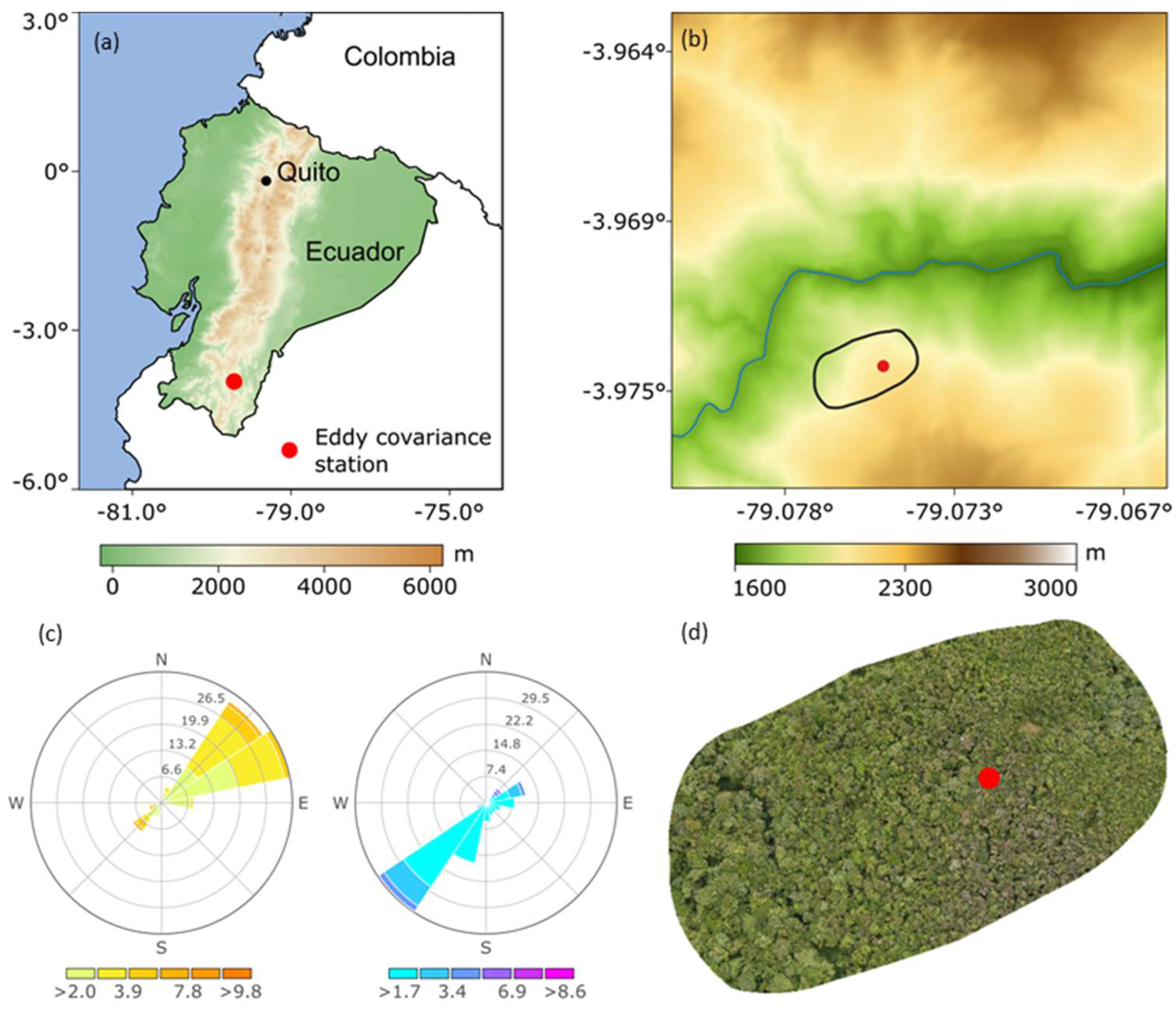
Figure 2.
Mean diurnal course of meteorological variables from January 2020 to December 2022: (a) wind speed (m/s, boxplot, blue), (b) friction velocity (u* m/s, orange), (c) wind direction (degree, blue), and (d) Monin-Obukhov stability parameter ((z-d)/L), blue).
Figure 2.
Mean diurnal course of meteorological variables from January 2020 to December 2022: (a) wind speed (m/s, boxplot, blue), (b) friction velocity (u* m/s, orange), (c) wind direction (degree, blue), and (d) Monin-Obukhov stability parameter ((z-d)/L), blue).
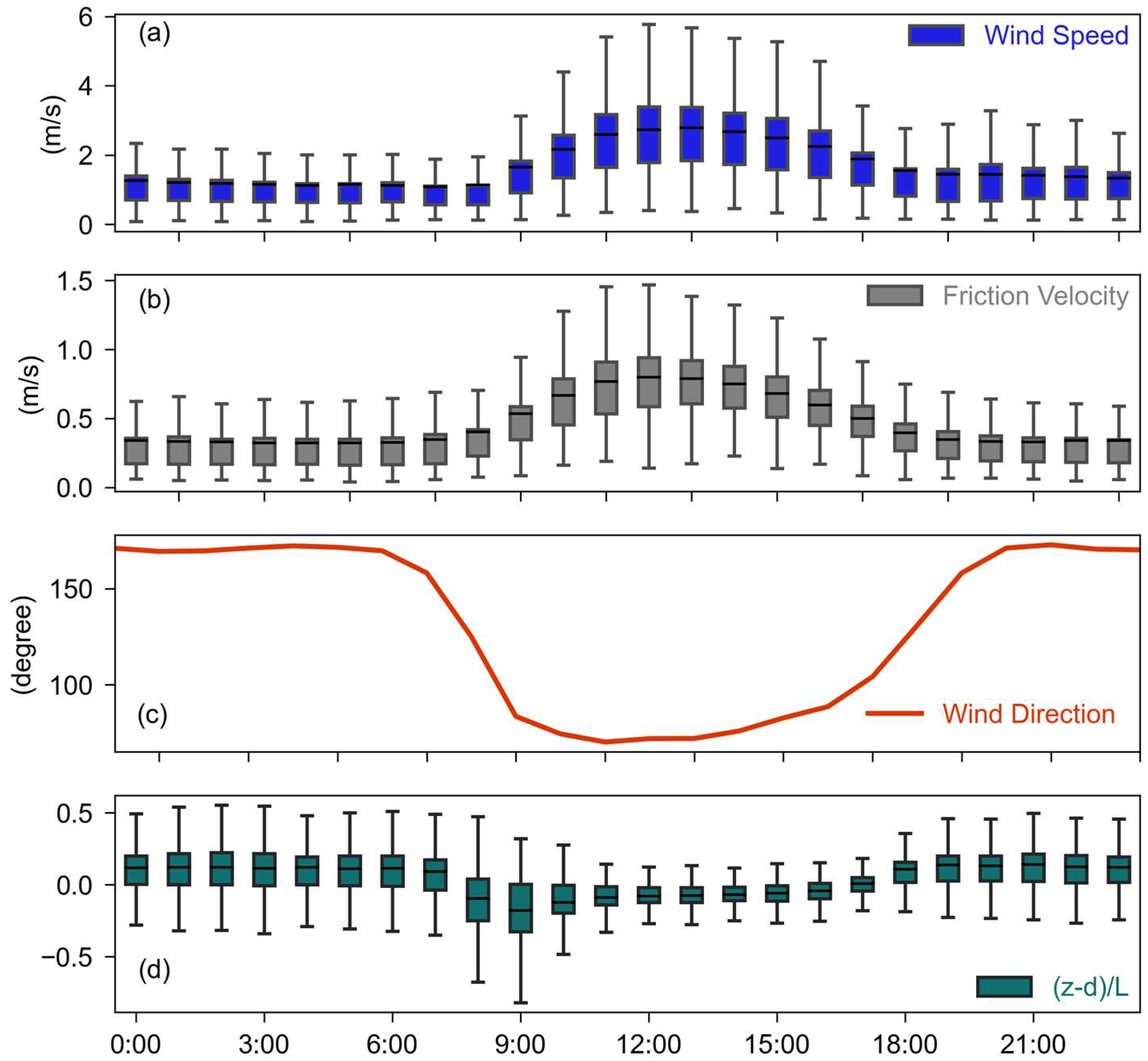
Figure 3.
Diurnal course of storage capacity indicated by (a) normalized air temperature (Tanorm) and (b) normalized relative humidity (RHnorm) at the height levels 1 = 1m, 2 = 6m, 3 = 12.5m and 4 = 19m.
Figure 3.
Diurnal course of storage capacity indicated by (a) normalized air temperature (Tanorm) and (b) normalized relative humidity (RHnorm) at the height levels 1 = 1m, 2 = 6m, 3 = 12.5m and 4 = 19m.
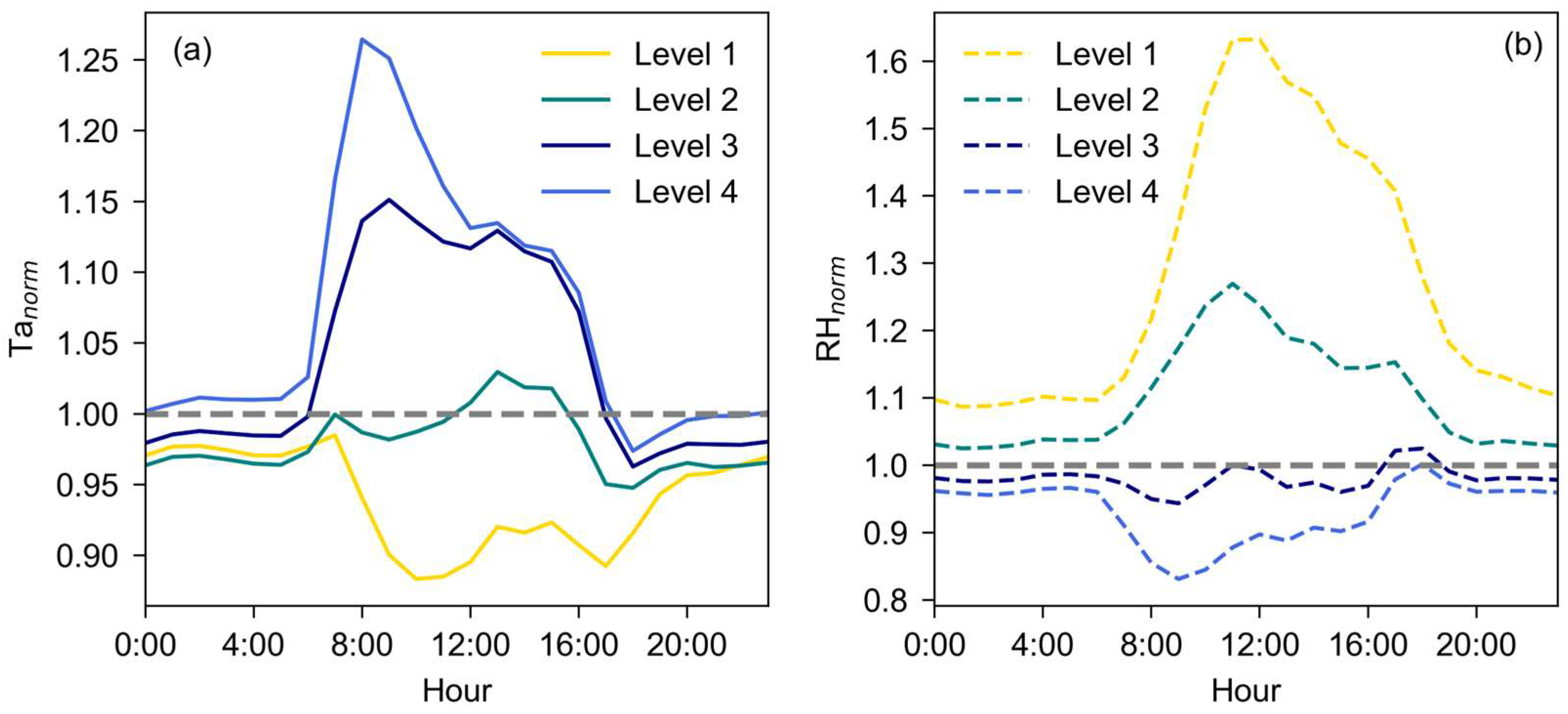
Figure 4.
(a) Linear fit of the sum of sensible heat (H, W/m²) and latent heat (LE, W/m²) against net radiation (Rn, W/m²) minus ground heat flux (G, W/m²), (b) diurnal cycle of LE (dark blue, W/m²), H (orange, W/m²), G (red, W/m²), corrected net radiation (Rn*, solid blue line, W/m²), and un-corrected net radiation (Rn, dashed blue line, W/m²) for the time period January 2020 – December 2022; (c) as (a), without the addition of the storage effect and with storage effect, (d) diurnal cycle of turbulent energy fluxes without storage (LE and H, W/m²) and with addition of storage ( SLE and SH,W/m²) for the time period October – December 2022.
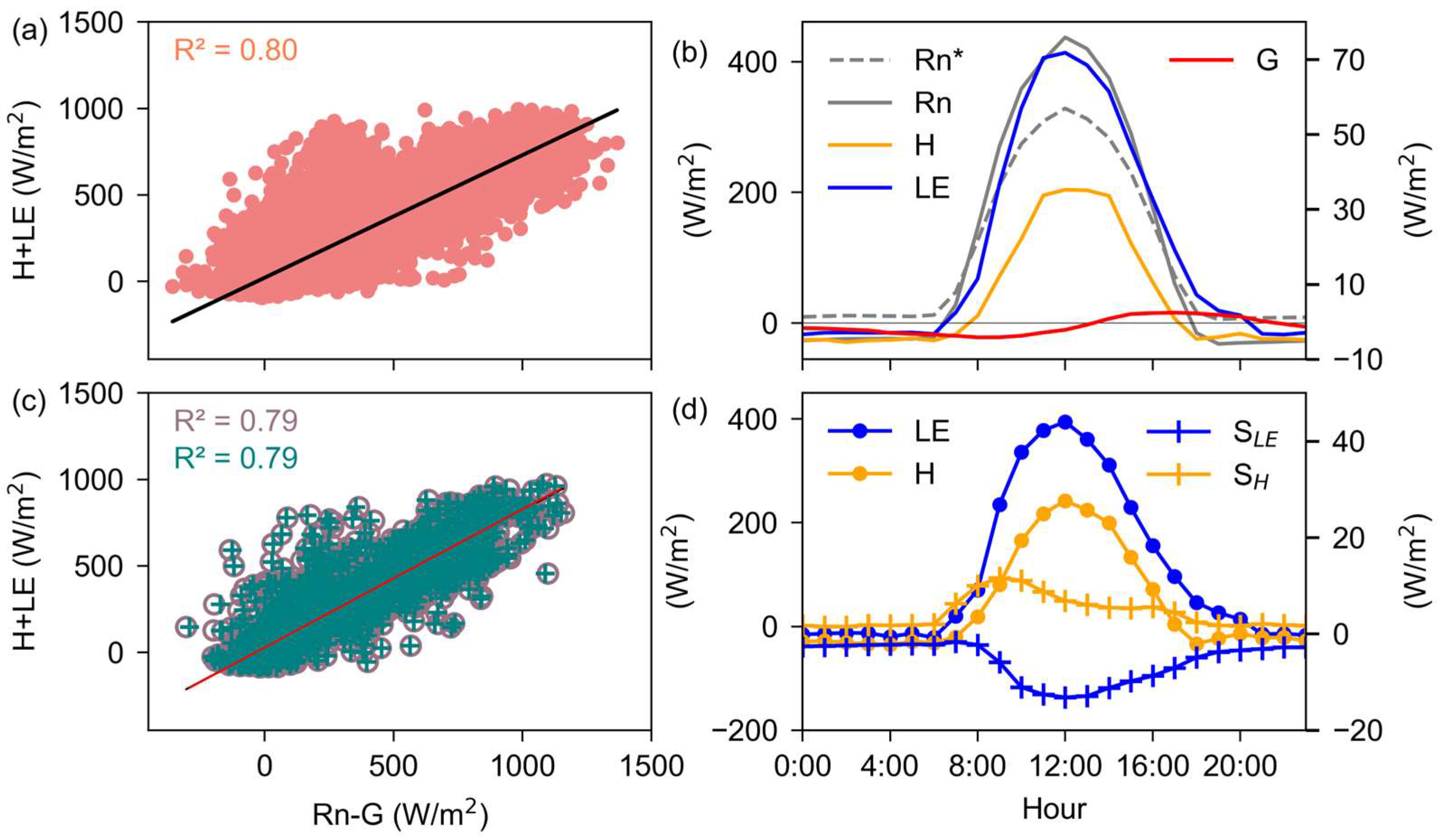
Figure 5.
Boxplots representing the diurnal course of (a) the residuals (ε, W/m², purple) for the time period January 2020 – December 2022, (b) the residuals without storage values (ε, W/m², red) and with addition of storage (ε’, W/m², cyan) for the time period October – December 2022.
Figure 5.
Boxplots representing the diurnal course of (a) the residuals (ε, W/m², purple) for the time period January 2020 – December 2022, (b) the residuals without storage values (ε, W/m², red) and with addition of storage (ε’, W/m², cyan) for the time period October – December 2022.
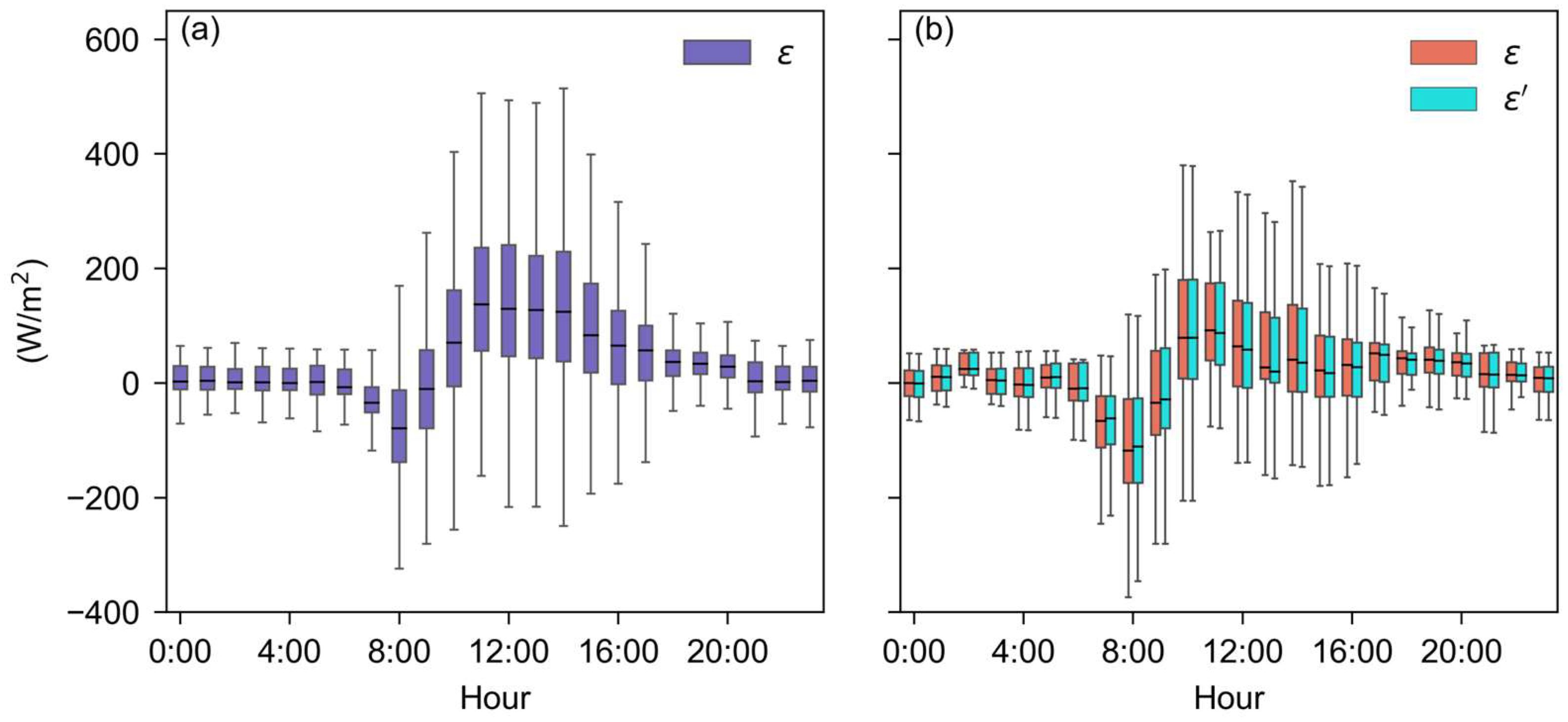
Figure 6.
Binned means of residuals (ε, W/m2) as a function of (a) Monin-Obukhov stability parameter (z-d)/L and (b) friction velocity (u*, m/s). Axis is subjected to differ for subplots.
Figure 6.
Binned means of residuals (ε, W/m2) as a function of (a) Monin-Obukhov stability parameter (z-d)/L and (b) friction velocity (u*, m/s). Axis is subjected to differ for subplots.
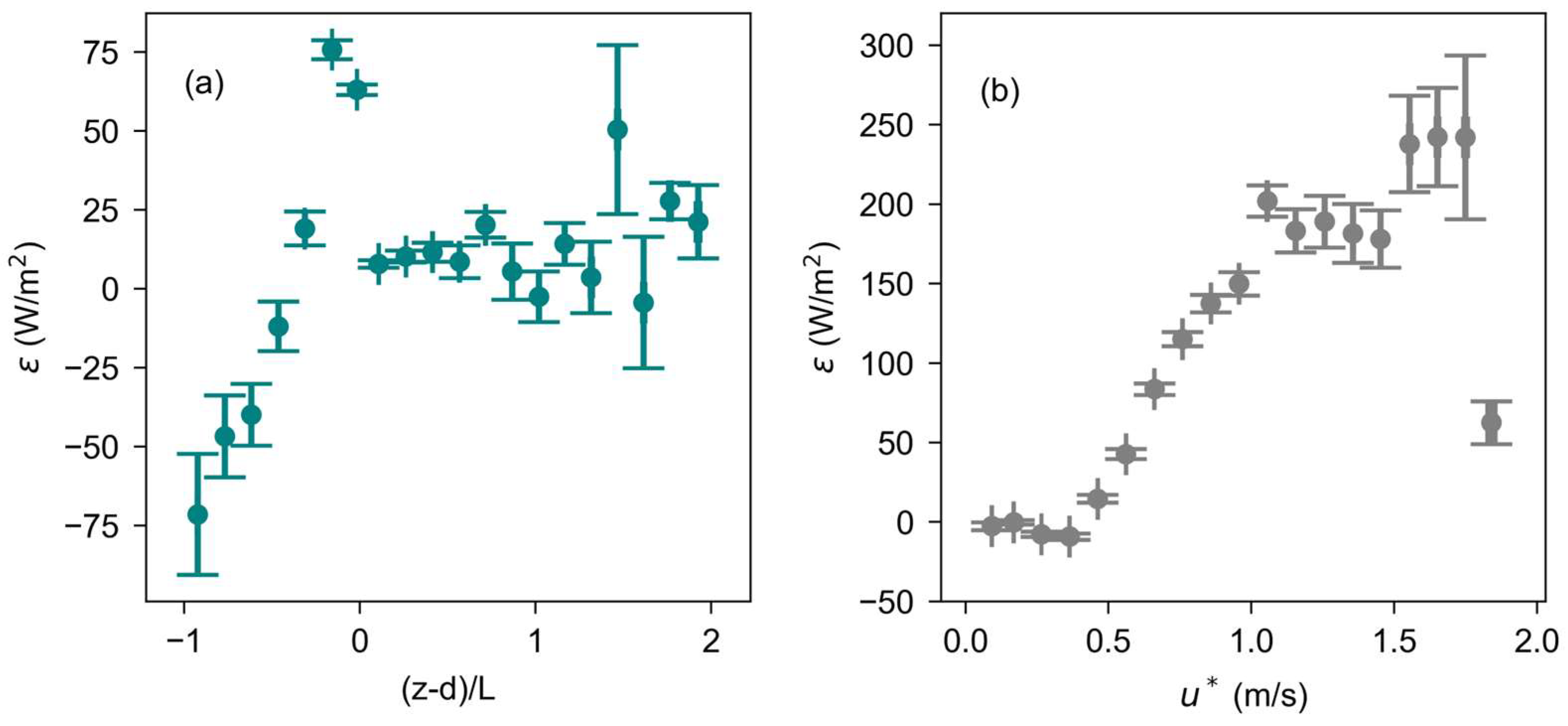
Figure 7.
Relationship of residuals (ε, W/m²) with (a) stability parameter ((z-d)/L, solid), (b) friction velocity (u*, dashed) at Daytime (orange line), Transition (green line), and Nighttime (blue line) as defined in Table 1.
Figure 7.
Relationship of residuals (ε, W/m²) with (a) stability parameter ((z-d)/L, solid), (b) friction velocity (u*, dashed) at Daytime (orange line), Transition (green line), and Nighttime (blue line) as defined in Table 1.
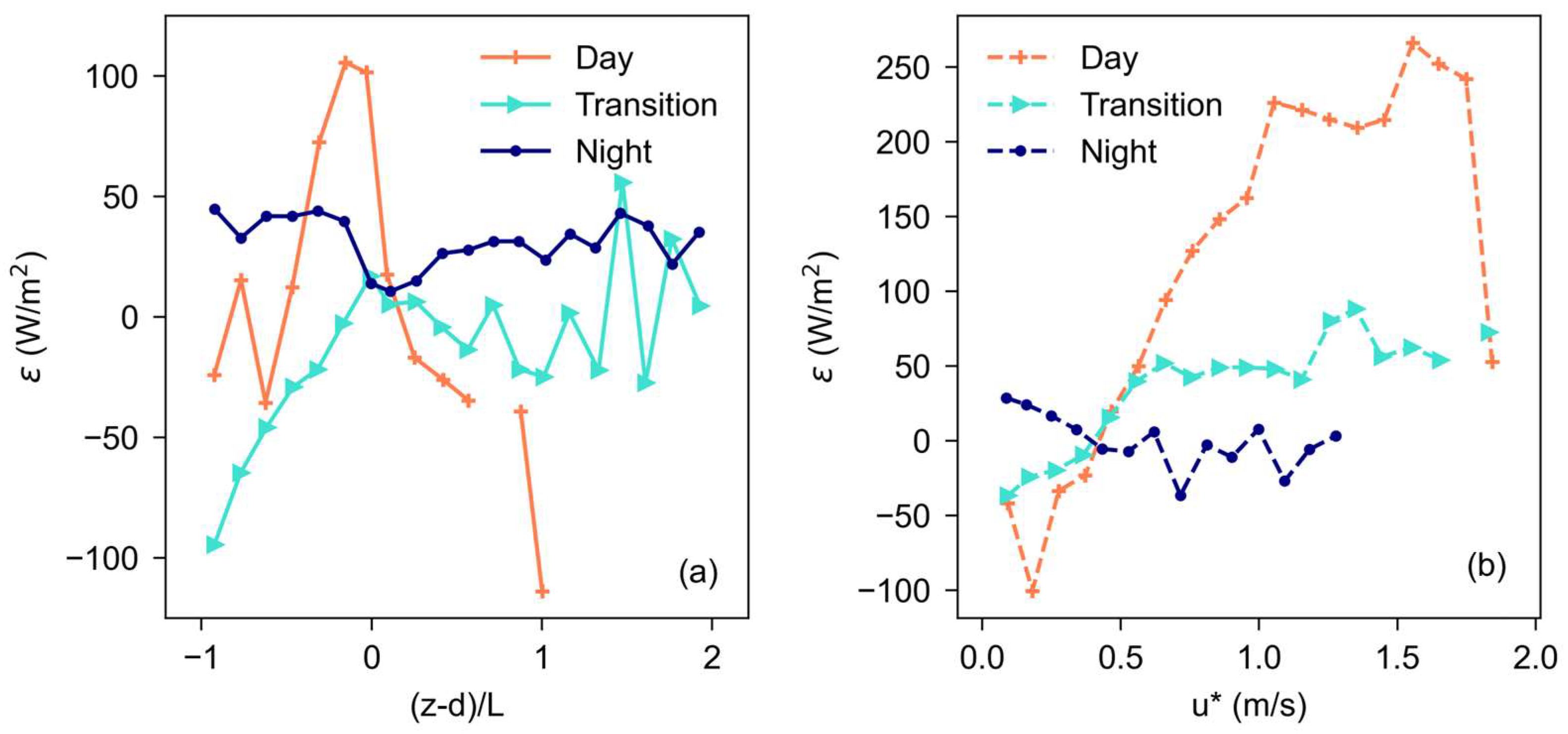
Figure 9.
Daily cycle of unfiltered net ecosystem exchange (NEE, solid line, μmol/m²hour) and filtered NEE* (dashed line, μmol/m²hour) for the entire time period.
Figure 9.
Daily cycle of unfiltered net ecosystem exchange (NEE, solid line, μmol/m²hour) and filtered NEE* (dashed line, μmol/m²hour) for the entire time period.
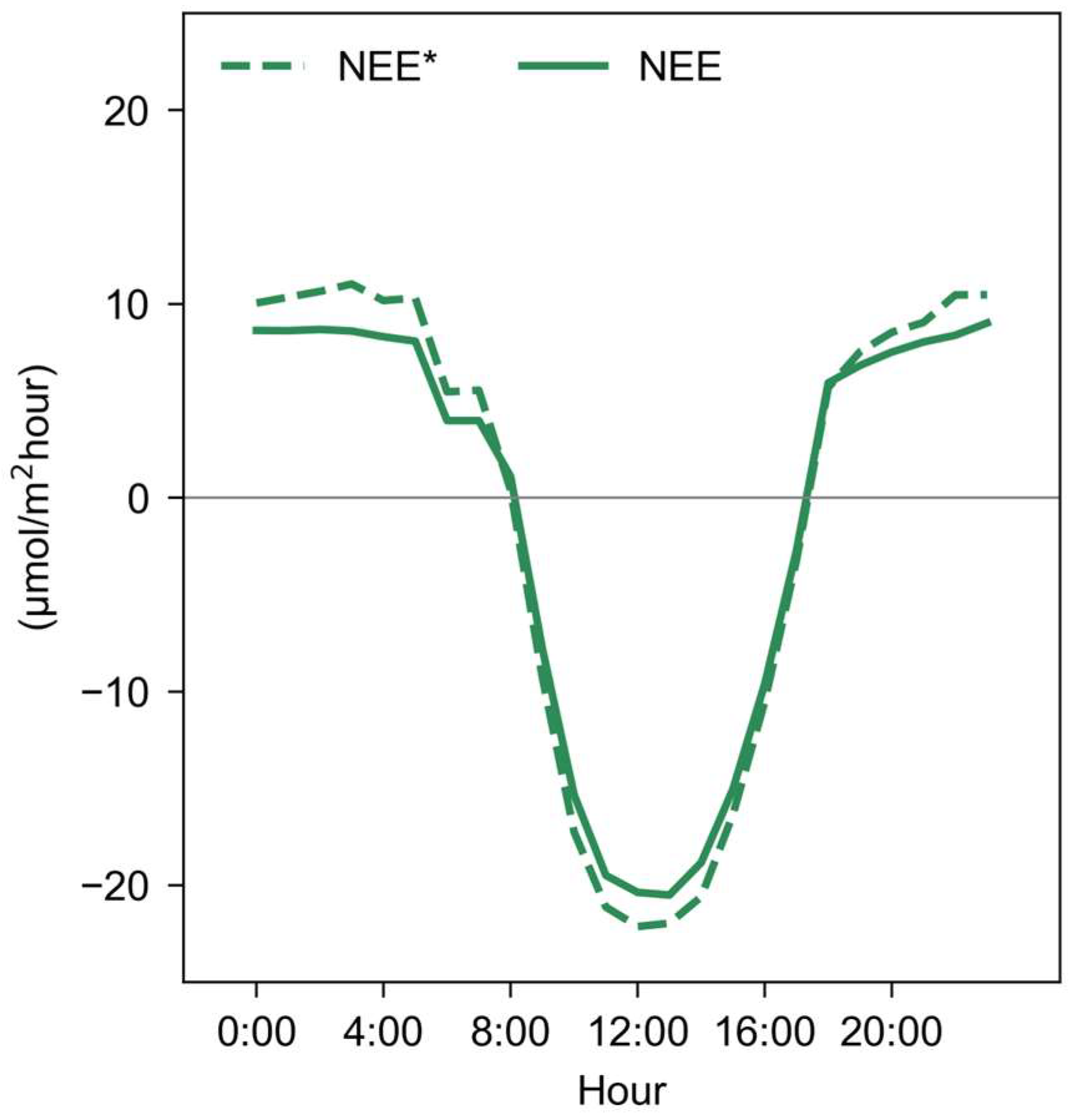
Figure 10.
Relationship between net ecosystem exchange (NEE) and (a) global radiation (Rg, W/m²) and (b) photosynthetic photon flux density (PPFD, mol/m²day). Daily means are used for analysis for specific time period between (8:00 – 16:00). Rg data span the entire period (January 2020 - December 2022), while PPFD data is limited to the period March 2022 - December 2022.
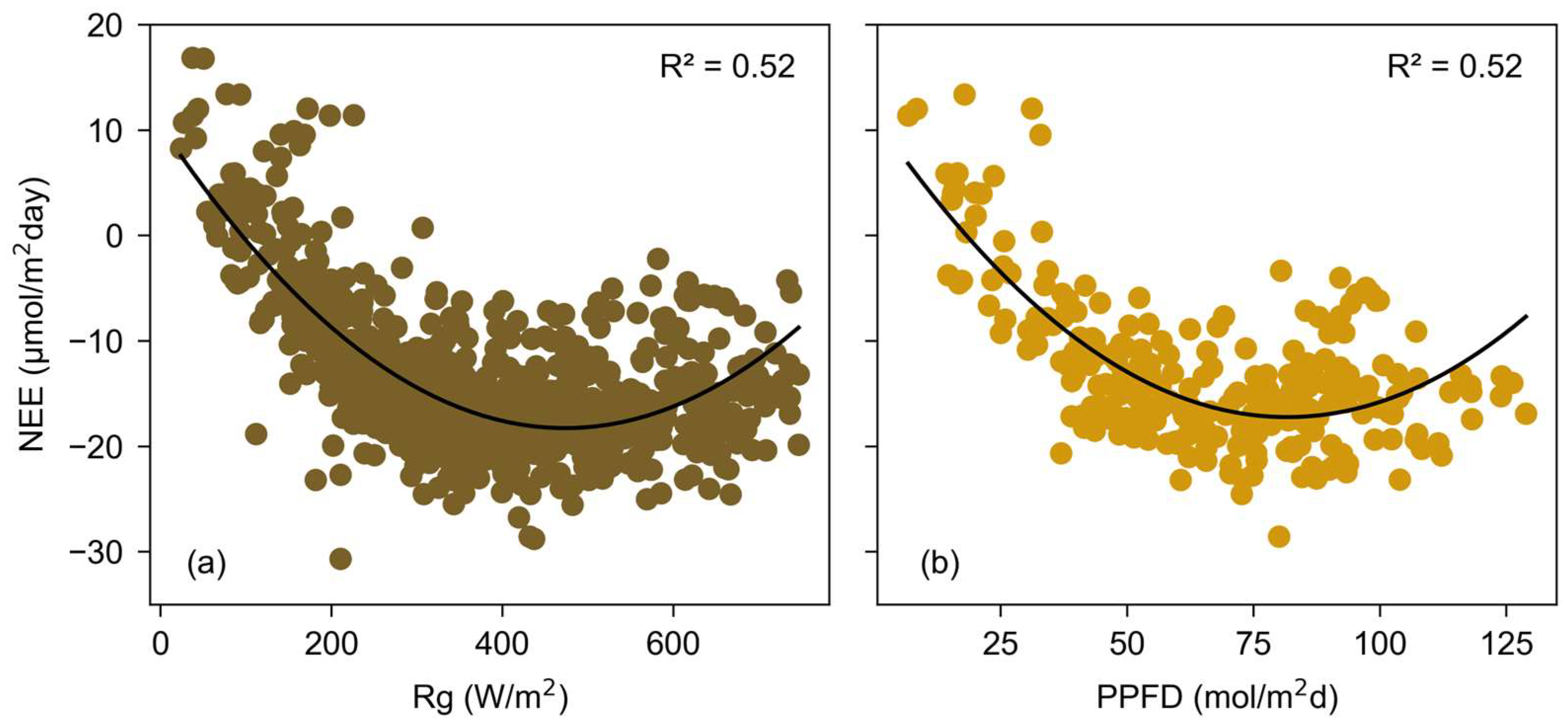
Figure 11.
Box plots representing the annual course of daily values for (a) air temperature (Ta, °C), (b) relative humidity (RH, %), (c) global radiation (Rg, W/m2), (d) sensible heat flux (H, W/m²), (e) latent heat flux (LE, W/m²), and (f) net ecosystem exchange (NEE, μmol/m²day).
Figure 11.
Box plots representing the annual course of daily values for (a) air temperature (Ta, °C), (b) relative humidity (RH, %), (c) global radiation (Rg, W/m2), (d) sensible heat flux (H, W/m²), (e) latent heat flux (LE, W/m²), and (f) net ecosystem exchange (NEE, μmol/m²day).
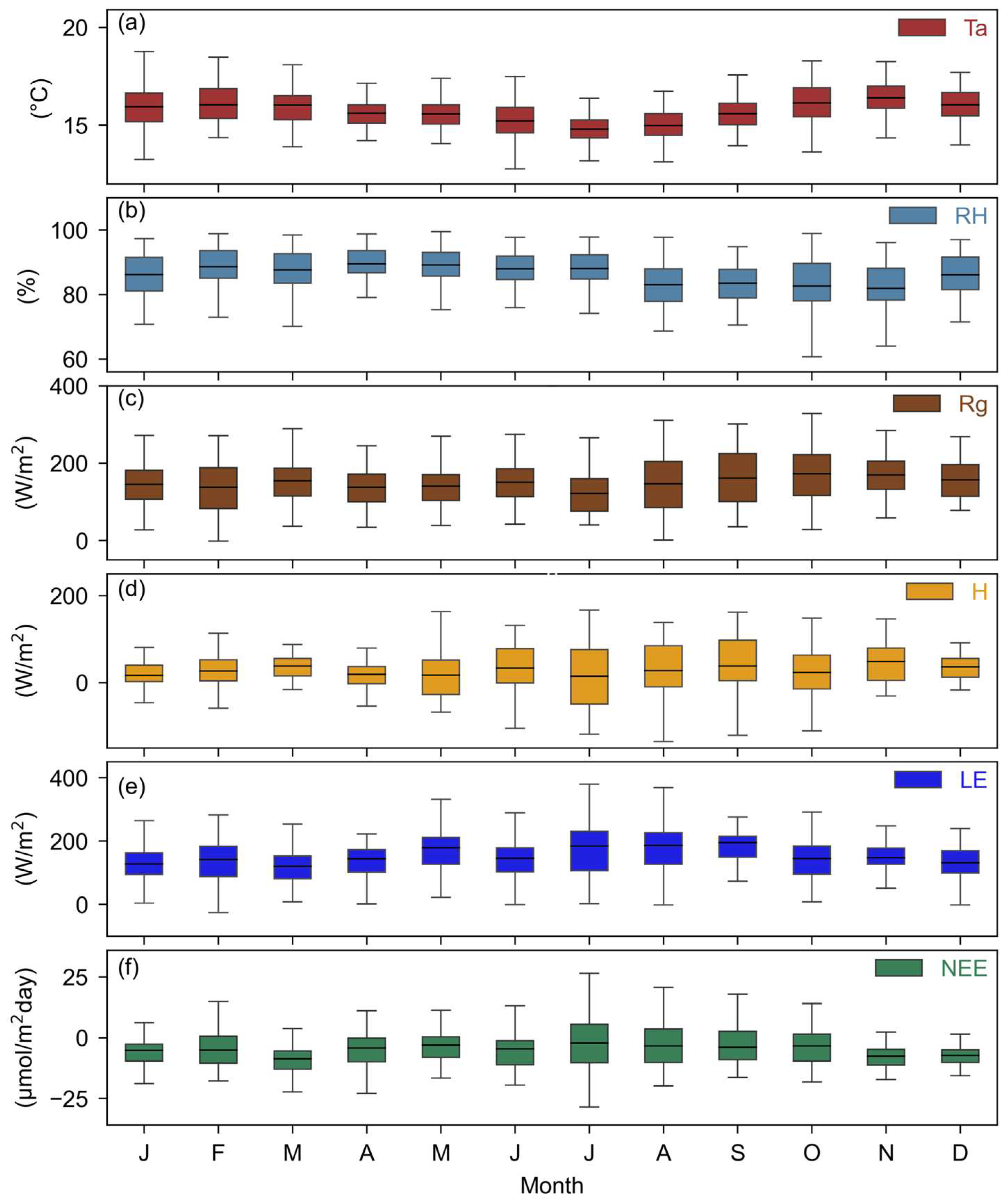

Table 1.
Remaining data availability in percentage after filtering. The data was divided as Day (11:00-14:00), Night (20:00–6:00) and Transition (07:00-10:00) and (15:00-19:00).
Table 1.
Remaining data availability in percentage after filtering. The data was divided as Day (11:00-14:00), Night (20:00–6:00) and Transition (07:00-10:00) and (15:00-19:00).
| Filtering | Time | NEE | H | LE |
|---|---|---|---|---|
| Precipitation | Day | 75% | 73% | 73% |
| Transition | 82% | 73% | 84% | |
| Night | 95% | 85% | 87% | |
| u* | Day | 67% | 60% | 60% |
| Transition | 48% | 58% | 58% | |
| Night | 34% | 21% | 21% |
Table 2.
Linear fits, explained variance (R²) and root mean square error (RMSE) of the sum of sensible heat (H, W/m²) and latent heat (LE, W/m²) as a function of available energy (Rn – G, W/m²) for H and LE without storage and with the addition of storage for the time period October 2022 – December 2022.
| Intercept | Slope | R² | RMSE | |
|---|---|---|---|---|
| Without storage | 27.71 | 0.79 | 0.786 | 121.37 |
| With addition of storage | 27.20 | 0.80 | 0.789 | 120.37 |
Table 3.
Mean and sum of the storage effect generated by the sensible heat flux (SH, W/m²), latent heat flux (SLE, W/m²) and EBC residual (ε, W/m²) calculated over the diel (all), daytime, nighttime and transition hours as defined in Table 1 for the time period October 2022 – December 2022.
Table 3.
Mean and sum of the storage effect generated by the sensible heat flux (SH, W/m²), latent heat flux (SLE, W/m²) and EBC residual (ε, W/m²) calculated over the diel (all), daytime, nighttime and transition hours as defined in Table 1 for the time period October 2022 – December 2022.
| SH (W/m²) | SLE (W/m²) | ε (W/m²) | ||||
| Mean | Sum | Mean | Sum | Mean | Sum | |
| All | 4.4 | 105.2 | -5.6 | -133.7 | 14.8 | 356.2 |
| Day | 6.8 | 27.1 | -12.5 | -49.9 | 56.9 | 227.8 |
| Night | 1.8 | 19.5 | -2.6 | -28.5 | 6.5 | 71.9 |
| Transition | 6.5 | 58.5 | -6.1 | -55.1 | 6.3 | 56.5 |
Table 4.
Linear fits, explained variance (R²) and root mean square error (RMSE) of the sum of sensible heat (H, W/m²) and latent heat (LE, W/m²) as a function of available energy (Rn – G, W/m²) for Day (11:00-14:00), Night (20:00–6:00) and Transition (07:00-10:00) and (15:00-19:00).
Table 4.
Linear fits, explained variance (R²) and root mean square error (RMSE) of the sum of sensible heat (H, W/m²) and latent heat (LE, W/m²) as a function of available energy (Rn – G, W/m²) for Day (11:00-14:00), Night (20:00–6:00) and Transition (07:00-10:00) and (15:00-19:00).
| Time period | Intercept | Slope | R² | RMSE |
|---|---|---|---|---|
| All data | 20.59 | 0.79 | 0.795 | 107.29 |
| Day | 135.8 | 0.56 | 0.545 | 133.32 |
| Night | -31.19 | -0.005 | -- | 22.17 |
| Transition | 33.39 | 0.67 | 0.666 | 108.36 |
Disclaimer/Publisher’s Note: The statements, opinions and data contained in all publications are solely those of the individual author(s) and contributor(s) and not of MDPI and/or the editor(s). MDPI and/or the editor(s) disclaim responsibility for any injury to people or property resulting from any ideas, methods, instructions or products referred to in the content. |
© 2024 by the authors. Licensee MDPI, Basel, Switzerland. This article is an open access article distributed under the terms and conditions of the Creative Commons Attribution (CC BY) license (https://creativecommons.org/licenses/by/4.0/).
Copyright: This open access article is published under a Creative Commons CC BY 4.0 license, which permit the free download, distribution, and reuse, provided that the author and preprint are cited in any reuse.


