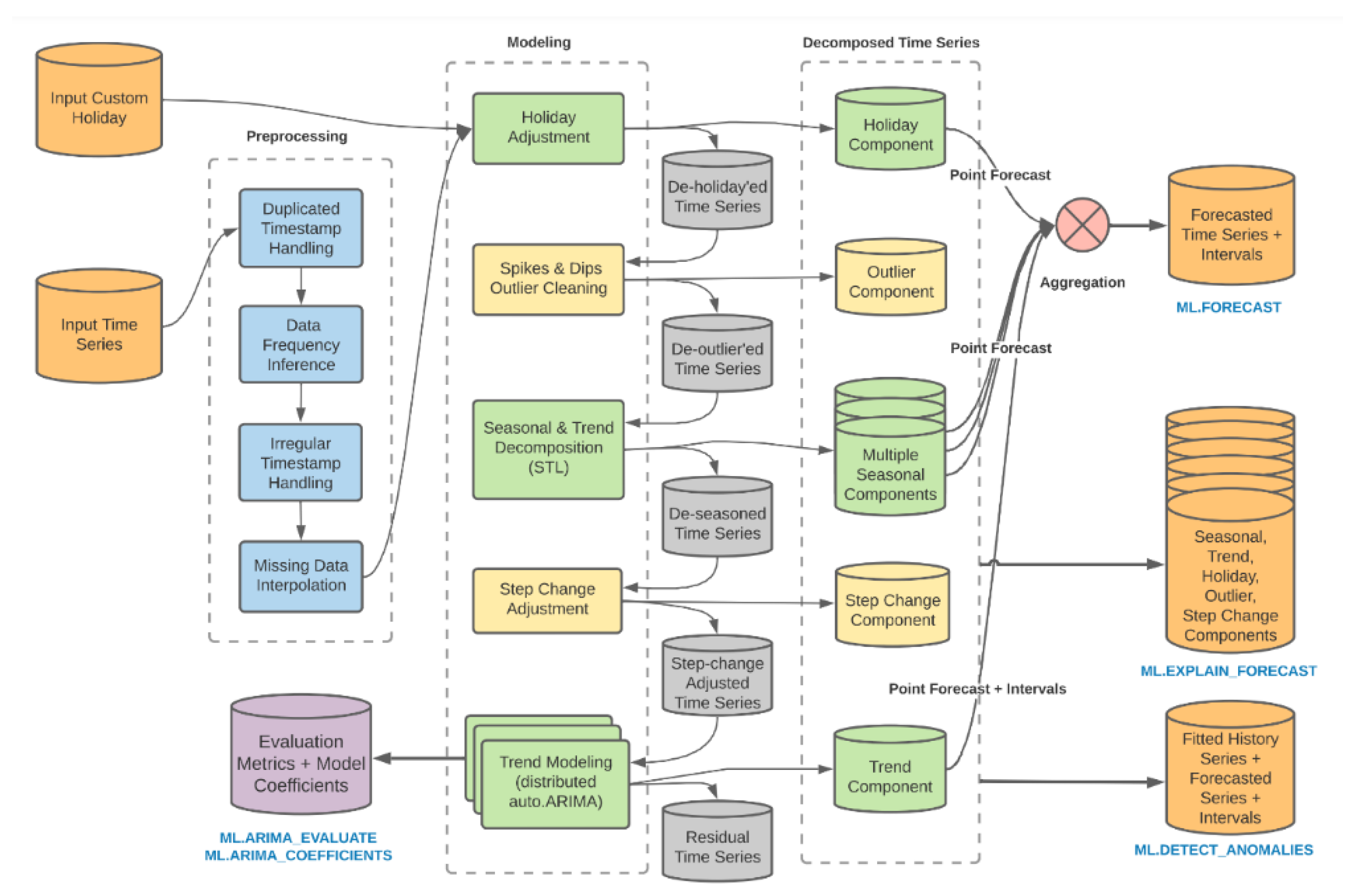
4. Results
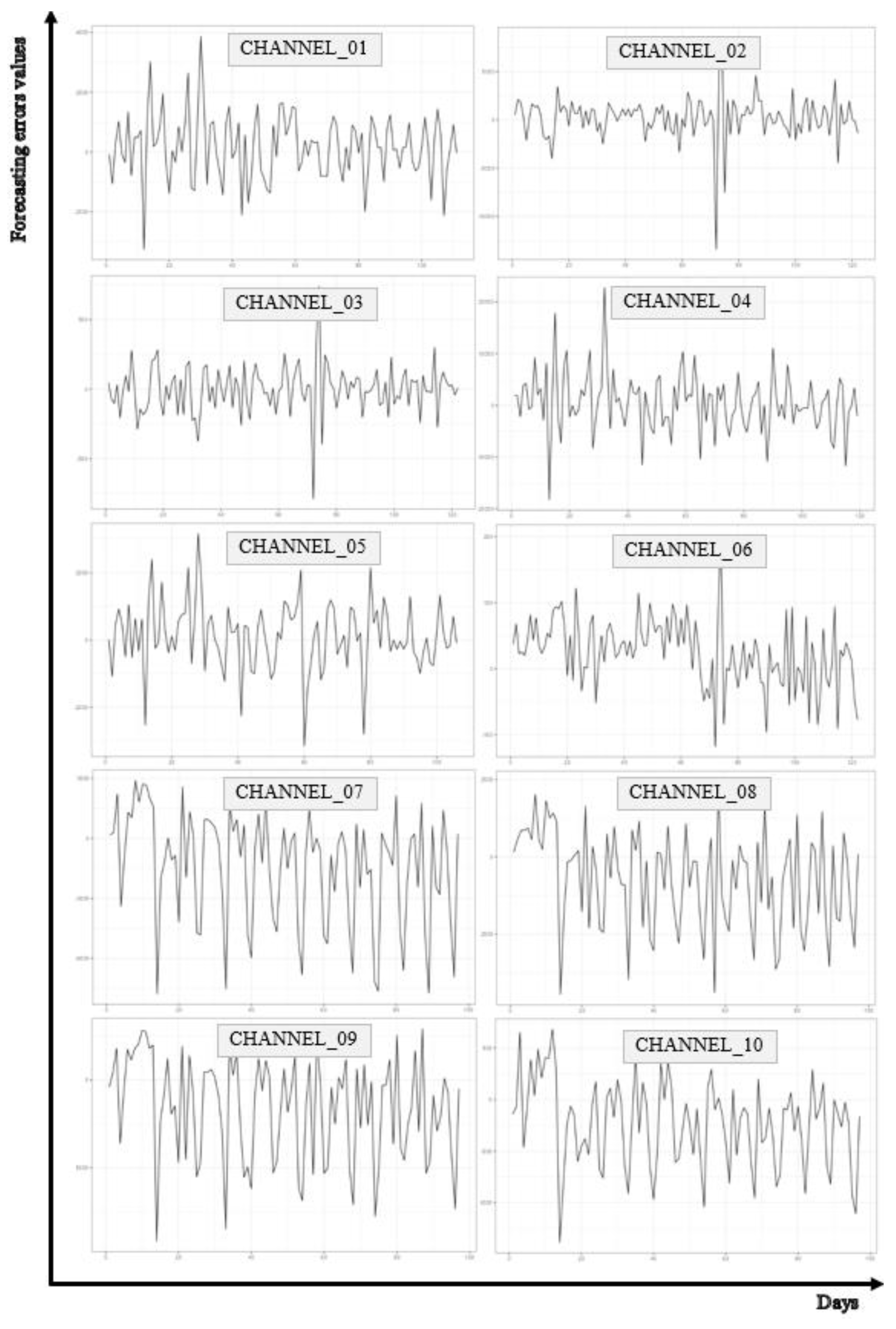
In the first step of the analysis, a visual assessment of the forecast error series was conducted. The visual analysis of time series forecast errors involves plotting these errors on a timeline. Such plots can reveal existing patterns, such as cyclicality, seasonality, or trends, which might not be evident in the analysis of the forecasted values alone. For example, if regular fluctuations are observed in the forecast error series over specific time periods, it may indicate that the forecasting model struggles to predict certain seasonal patterns. The progression of the analyzed time series is presented in
Figure 4.
The visual analysis of time series forecast errors is a crucial phase in examining forecasting models. By thoroughly understanding the patterns and properties of error series, researchers and analysts can identify significant relationships and aspects that merit further, more detailed investigation. This approach enables a deeper understanding of the dynamics of forecast errors and potential issues within the models. Following the visual analysis, it becomes possible to conduct more advanced statistical analyses. Calculating basic distribution parameters of forecast errors, such as the mean, standard deviation, or skewness, can provide insights into the characteristics and asymmetry of the errors. Furthermore, STL decomposition (Seasonal and Trend decomposition using Loess) allows for the extraction of trend, seasonality, and remainder components, which can help identify the primary sources of errors in forecasts. Statistical hypothesis testing also plays a critical role in the analysis. Determining p-values for tests under the null hypothesis of no trend or seasonality helps establish whether statistically significant deviations from these assumptions exist. The basic numerical characteristics of the analyzed forecast error time series are presented in
Table 4..
The time series analysis of forecast errors for different channels revealed diverse patterns and characteristics of errors in these channels. Some channels tend to overestimate, while others tend to underestimate forecasted values. Differences in standard deviation, coefficient of variation, skewness, and kurtosis indicate the diversity of error variability. For each channel, analyzing these parameters can provide valuable insights for further optimization and improvement of forecasting models. For Channel_01, the mean error is 176, and the median is 172, which suggests that most errors are below the mean value. However, the skewness coefficient indicates weak asymmetry in the error distribution. Nevertheless, the large standard deviation (1095) and high coefficient of variation (CV = 6.212) indicate significant error variability. For Channel_02, the mean error is 245, and the median is 507, which suggests that the models tend to underestimate predicted values. High values of standard deviation (2268) and kurtosis (11.280) indicate significant variability in the error distribution. In the case of Channel_03, the mean error is close to zero, but the low median (15.5) and large standard deviation (174) suggest that the errors have diverse characteristics. Skewness is close to zero, while kurtosis (4.387) indicates a higher concentration of values than in a normal distribution (kurtosis = 0). For Channel_04, the mean error is 574, and the median is 297, which indicates underestimation of predicted values. High values of standard deviation (5665) and kurtosis (2.270) indicate significant error variability and some degree of dispersion of the analyzed values. The distribution is positively skewed. The mean error in Channel_05 is 126, and the median is 149, which suggests slight underestimation of values. High values of standard deviation (1017) and coefficient of variation (CV = 8.040) indicate significant variability. The error distribution is negatively skewed. For Channel_06, the mean error is 25, and the median is 29.5, which suggests slight underestimation of values. Low standard deviation (52) and kurtosis (0.567) indicate relatively low variability and closeness to normality in the distribution. The error distribution is negatively skewed. The mean error for Channel_07 is negative (-1387), and the median is also negative (-687), which indicates a tendency to overestimate predicted values. High values of standard deviation (2822) and kurtosis (-0.487) indicate significant error variability and platykurtosis of the distribution. The distribution is negatively skewed. Channel_08 is characterized by a mean error of -706 and a median of -175, which suggests overestimation of predicted values. High values of standard deviation (1602) and kurtosis (-0.774) indicate some variability in errors and platykurtosis of the distribution. The distribution is negatively skewed. In the case of Channel_09, the mean error is negative (-1583), and the median is also negative (-732), which suggests overestimation of predicted values. High values of standard deviation (2969) and kurtosis (-0.726) indicate significant error variability and platykurtosis of the distribution. The distribution is negatively skewed. For Channel_10, the mean error is -228, and the median is -147, which suggests overestimation of predicted values. High values of standard deviation (420) and kurtosis (-0.354) indicate variability in errors. The distribution is negatively skewed. In general, the coefficient of variation (CV = Std.Dev / Mean) indicates high variability in the distributions of the analyzed errors.
In the next step of the analysis, the randomness of forecast errors was examined. The results are presented in
Table 5..
The analysis of the randomness of forecast errors indicates that each of the analyzed series can be considered random (in the sense of one of the applied tests and with alpha = 0.05). However, low p-value values for Channel_02, Channel_07, Channel_09, and Channel_10 in some tests may suggest the presence of certain patterns in the error progression. The stationarity analysis of the considered error series using the ADF (Augmented Dickey–Fuller test) indicates that the series can be considered stationary (p-value <= 0.01 for each series). The results of the autocorrelation analysis of the examined series are not uniform and may indicate the presence of autocorrelation. Detailed values of coefficients and critical significance levels (p-values) for the first seven lags are presented in
Table 6. The analysis utilized ACF coefficients and the Ljung-Box test.
Preliminary analyses indicate that patterns may be present in each of the considered series. In each case, autocorrelation can be observed for the first seven lags. The summary of the analysis results for the examined forecast error time series is presented in
Table 7,
Table 8 and
Table 9.
In
Table 7, the individual columns present the following information:
- “Trend_stl” – Value calculated using formula (3), indicating the strength of the trend component in STL decomposition (the closer the value is to 1, the more significant the trend component in the error).
- “Season_stl” – Value calculated using formula (4), indicating the strength of the seasonal component in STL decomposition (similarly, the closer the value is to 1, the more significant the seasonal component in the error series).
- “MAE_error” – The MAE error value (1) for a given product.
- “MAPE_error” – The MAPE error value (2) for a given product.
- “Remainder_MAE_stl” – The “non-systematic” error, understood as the MAE value of the error series calculated for the remainder component in STL decomposition (the mean of the absolute values of the remainder component of the error series), indicating the MAE error excluding systematic components of the error series.
- “Iloraz_stl” – The relative “non-systematic” error, calculated as the ratio of “Remainder_MAE_stl” to “MAE_error”, indicating what portion of the total MAE error is represented by the MAE calculated solely for the remainder component of STL decomposition.
The data in the table is arranged in non-decreasing order of the value of measure (4), which determines the strength of the seasonal component in the error series. In STL decomposition, a frequency of 7 was adopted for each analyzed series, as the operator works 7 days a week, and the data pertains to daily volumes. The results presented in
Table 7 do not reveal direct, strong, and unambiguous relationships between the listed quantities. Only the following correlations (Pearson's, alpha = 0.05) can be considered significant:
1. Between the strength of the trend component (Trend_stl) and the strength of the seasonal component (Season_stl), r = 0.59 (t = 2.426, p = 0.034). The more significant the trend component, the more significant the seasonal component.
2. Between the strength of the trend component (Trend_stl) and the relative “non-systematic” error (Iloraz_stl), r = -0.69 (t = -3.163, p = 0.009). The more significant the trend component in errors, the smaller the error associated with excluding this component.
3. Between the strength of the seasonal component (Season_stl) and the relative “non-systematic” error (Iloraz_stl), r = -0.70 (t = -3.251, p = 0.007). The more significant the seasonal component, the smaller the “non-systematic” error.
4. Between the “non-systematic” error (Remainder_MAE_stl) and the MAE error (MAE_error), r = 0.88 (t = 6.185, p < 0.001). The greater the absolute error, the greater the absolute “non-systematic” error. This relationship can generally be considered obvious.
Regarding the first point, it should be noted that in the analyzed series, the maximum value of indicator (3) is 0.158, generally indicating a weak trend component in the analyzed error series. Only in two cases is the strength of the trend component greater than the strength of the seasonal component (Channel_02, Channel_09). In the considered problem, the seasonal component of the error series is of greater importance. Particular emphasis should be placed on the numerical aspects of the method for extracting systematic components using STL. The identified trend is generally non-linear, and changes to decomposition parameters can control trend variability. At the same time, this is closely related to the seasonal component, with practically no influence on the remainder component. From this perspective, systematic components should be considered together. For predefined decomposition parameters, correlations between systematic components naturally occur. Therefore, the correlations presented in points two and three should be treated as natural. Despite the generally weak trend component, the results of trend detection using Student's t-test, Mann–Kendall test, and WAVK test (Lyubchich V. et al. 2023) indicate significant trends in most of the analyzed series. Detailed results are presented in
Table 8.
The results presented in
Table 8 indicate the presence of a trend in forecast errors for channel_02, channel_07, channel_08, and channel_09. However, based on visual assessment of the phenomenon over time, a distinct trend cannot be confirmed. To examine the presence of a significant seasonal component in the analyzed time series, the following tests were used: combined.kwr - Ollech and Webel's combined seasonality test (Ollech, D.; Webel, K.; 2020), test QS (qs.p), Friedman Rank test (fried.p), Kruskal-Wallis test (kw.p), F-Test on seasonal dummies (seasdum.p), Welch seasonality test (welch.p).
The results of the conducted tests indicate a clear presence of seasonality in the error series for channel_10, channel_07, and channel_08. For channel_09, low p-value values also suggest the possibility of significant seasonality. These results are consistent with those obtained in the analysis of the strength of the seasonal component (4).
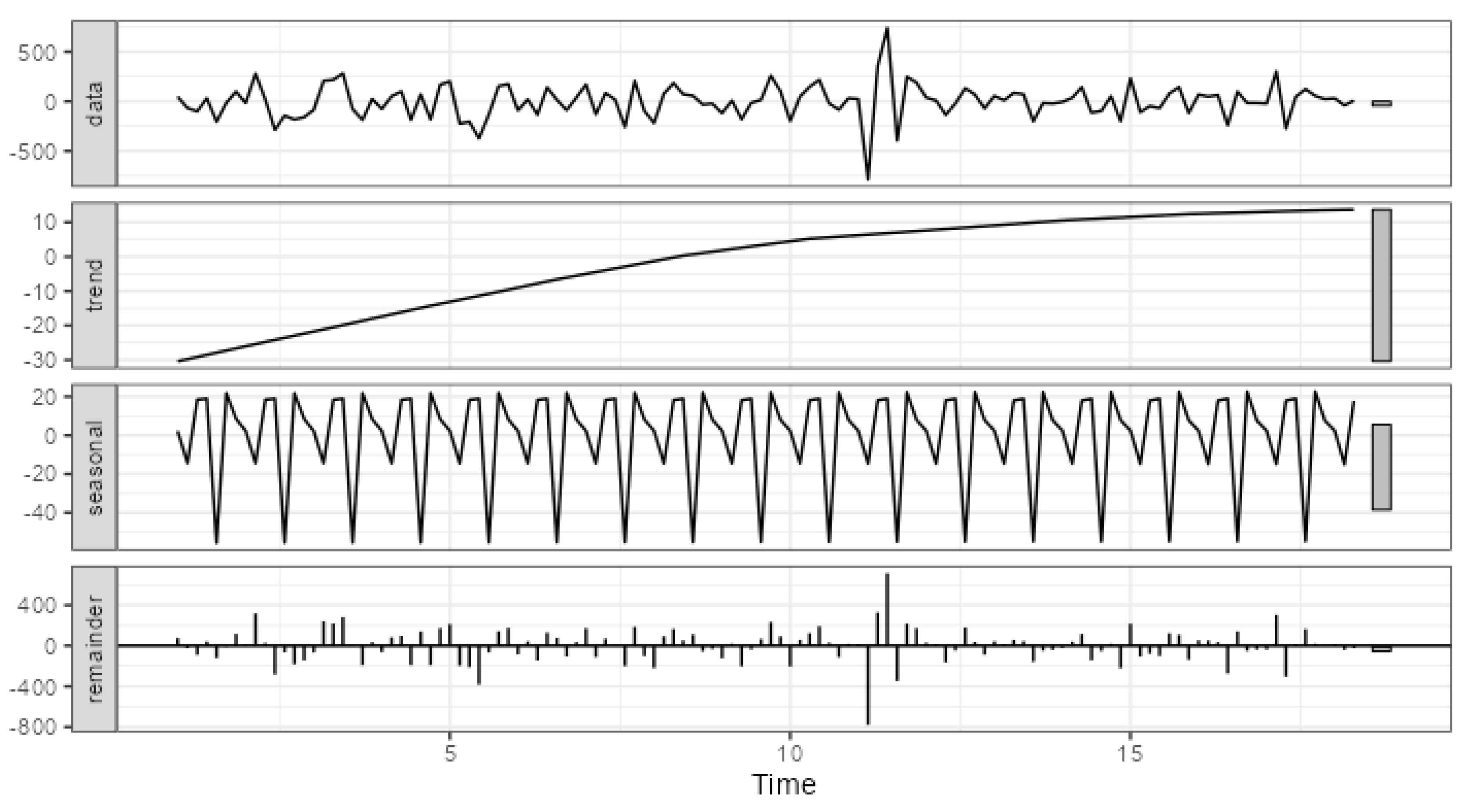
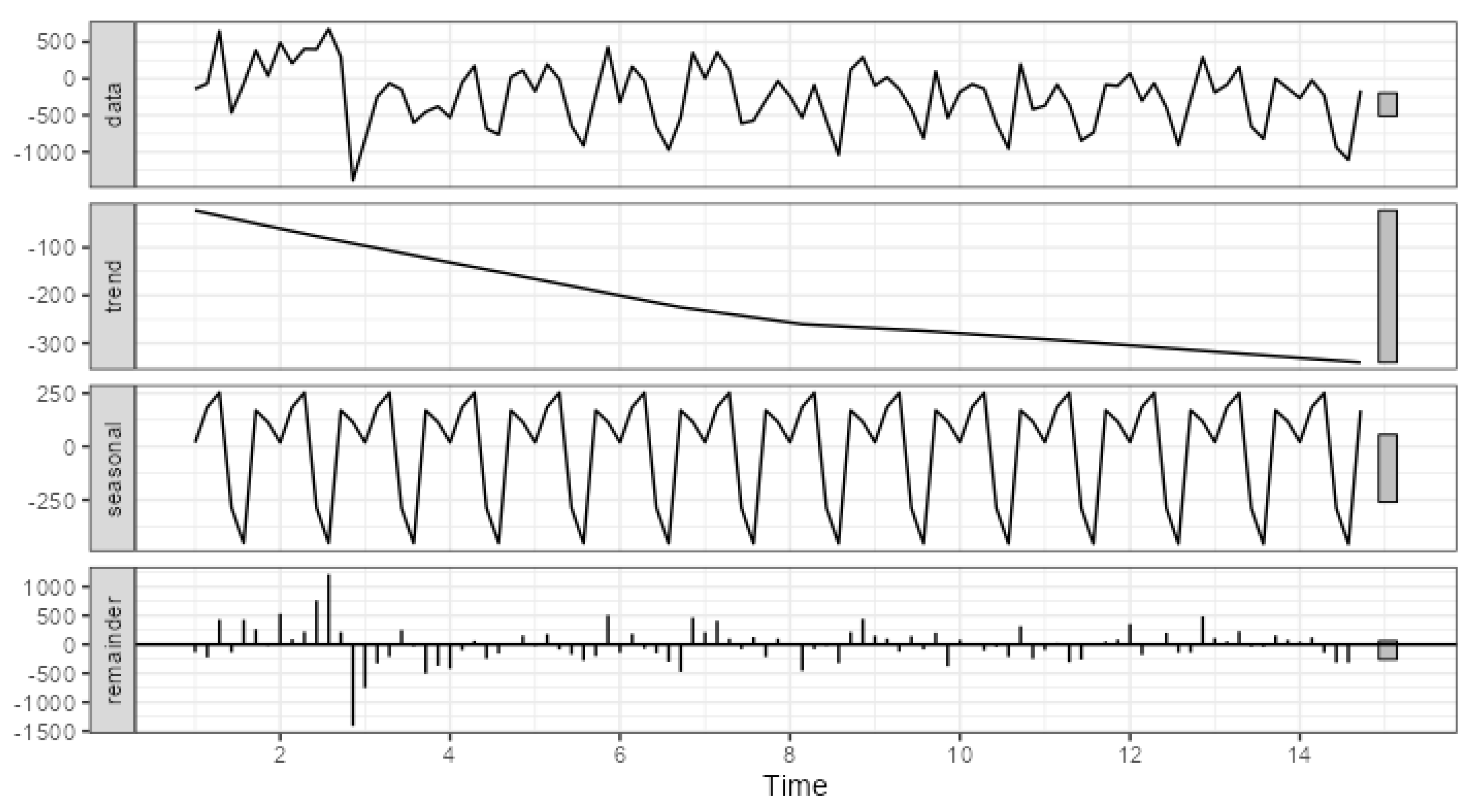
Figure 5 and
Figure 6 present visualizations of the conducted decompositions for two extreme examples.
Figure 5 shows the decomposition of errors for channel_03, which has the smallest proportion of systematic components in the total error.
Figure 6, on the other hand, presents the decomposition of errors for channel_10, which has the largest proportion of systematic components.
The primary difference in the strength of systematic components can be attributed to the scale of errors. In the case of channel_03, the trend component ranges from approximately -30 to 10, the seasonal component from approximately -56 to 23, while the range of total error variation is from -786 to 740. For channel_10, the trend component ranges from approximately -340 to -23, the seasonal component from approximately -457 to 253, and the range of total error variation is from -1388 to 681. Thus, the visualization of error decomposition can also be used to assess the strength and significance of systematic error components. It should be noted that the range of changes in individual components can serve as a key indicator in this context.
In summary, the obtained results highlight that significant systematic components in error series were identified in all examined channels of the household equipment manufacturer—significant seasonality in all channels and the absence of a significant trend only in channel 10. Regarding the distribution channels for pharmaceutical products, a significant systematic component (trend) was identified only in channel 2.