2. Theoretical Background
2.1. Demand Forecasting by Logistics Operators
One of the most common strategies for determining future demand levels is the use of forecasting methods. Forecasts are critical inputs for decision-making in procurement, production, delivery, and inventory management (Alam and El Saddik, 2017). They enable efficient production and raw material planning, preventing shortages that could lead to delivery delays and increased production costs. Accurate forecasting also facilitates cost optimization by determining the optimal quantities of raw materials and delivery schedules, thus reducing storage costs and avoiding excess inventory. Abolghasemi et al. (2020) agree with this view, emphasizing areas such as demand planning, inventory replenishment, production planning, and inventory control as key domains where forecasts support managerial decision-making. A well-constructed forecasting system ensures the smooth flow of goods across production stages, warehouses, and sales points, enabling timely and cost-efficient distribution. Additionally, forecasts support modern logistics concepts like mass customization (Guo et al., 2019). They also help adapt to changing market conditions, such as shifts in demand, raw material prices, or regulatory changes, ensuring organizations can respond swiftly to market dynamics.
Demand forecasting should support aggregation over short-, medium-, and long-term horizons (Kim et al., 2019). The ability to easily aggregate forecasts across time horizons, geographies, and product lines allows for customization based on individual client requirements. The foundation of an effective forecasting system is a well-defined strategy that includes the selection of appropriate forecasting methods and information flow processes. Popular algorithms for demand forecasting in logistics flows include ARIMA-based models (Abolghasemi et al., 2020), machine learning (Chen and Lu, 2021), and neural networks (Kim et al., 2019). However, due to the frequent unavailability of high-quality input data or challenges in automating forecasting processes, many forecasts are still created or adjusted based on human judgment. As noted by Perera et al. (2019), the human factor plays a critical role in forecast reliability. The most influential factors affecting forecast quality include product history, promotional schedules (Ma et al., 2016), as well as distribution network coordination and relationships within the network. Forecasting is increasingly being associated with logistics operators, who are often tasked with forecasting the financial feasibility of certain initiatives (Wang et al., 2018) or operational activities such as cross-docking forecasts (Grzelak et al., 2019). However, these approaches tend to focus on specific operational aspects rather than broader network-wide applicability.
The growing complexity of distribution networks, particularly with the rise of omnichannel systems (Briel, 2018), provides further impetus for developing forecasting systems at the logistics operator level. In this context, operators assume the role of coordinators for logistics processes (Kramarz and Kmiecik, 2022). Centralization of forecasting within distribution networks is one concept that expands the functions of logistics operators. Centralization can be considered in terms of transportation, operations, or decision-making processes (Simoes et al., 2018). It is often linked to trust and the ability to track flows (Beikverdi and Song, 2015; Lu and Hu, 2018). In this article, centralization is examined from the perspective of implementing processes that allow a single network node to assume decision-making functions and the collection and analysis of information. Key drivers for centralization include the diverse nature of activities within organizational units, the lack of designated entities responsible for coordinating demand management with other processes, and the vertical structure of organizations that exacerbates independent decision-making on demand management across entities (Szozda and Świerczek, 2016). The centralization concept posits that a logistics operator, equipped with the necessary attributes, can assume centralized forecasting functions in a distribution network. This reduces the burden on manufacturers to create demand forecasts and amplifies the benefits of producer specialization. The implementation of centralized forecasting by logistics operators has been conceptually explored (Kmiecik, 2021a), and implementation guidelines have been developed for designing and adopting forecasting models within logistics outsourcing companies (Kmiecik, 2021b). Currently, a forecasting tool designed by the author is being piloted by an international logistics operator.
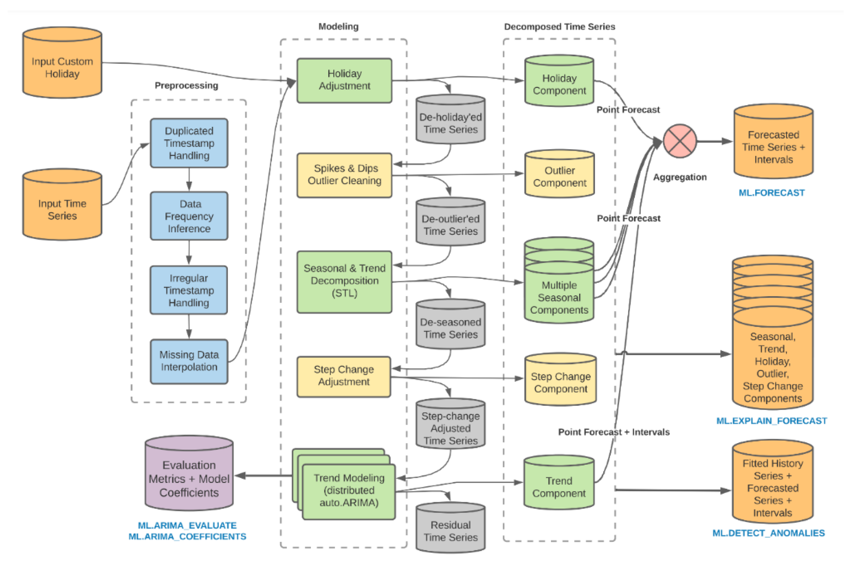
The potential benefits of such solutions can significantly impact the entire distribution network. In appropriate conditions, logistics operators could forecast demand as part of a broader demand management system. This would create a foundation for actions such as sales planning, inventory allocation, and production scheduling across the network. Operators could leverage their expertise in flow management to coordinate these activities. Furthermore, demand forecasts play an essential role in operational planning, such as resource allocation in warehouse management (Kmiecik and Wolny, 2022). Whether forecasts are used to coordinate network-wide flows or support the operator's operations, they must demonstrate a high level of accuracy. Accurate demand forecasts are vital for effective supply chain and production management, enabling precise planning, cost optimization, improved service quality, and enhanced customer satisfaction. Accurate forecasting helps avoid shortages, reduces storage costs, minimizes excess inventory, and ensures business continuity. One way to improve forecast accuracy is by analyzing the errors generated by the current forecasting system, which in this case is based on ARIMA_PLUS models offered by Google Cloud AI. Methodological elements of the forecasting tool are presented in
Figure 1.
It is worth emphasizing that the forecasting system should be treated as a black box. While it is possible to control certain parameters or modules of the tool, the precise identification and definition of the models used to generate forecasts remain inaccessible. The tool’s utility lies in its proper calibration. From this perspective, analyzing the generated errors takes on particular significance.
2.2. Analysis of Forecasting Errors
The analysis of forecasting errors is a critical tool in the field of forecasting, enabling the evaluation of the effectiveness of adopted models in predicting future events. This process involves comparing the actual observed values of a studied phenomenon with the predicted values generated by the forecasting model. By identifying discrepancies between predictions and reality, researchers can gain a deeper understanding of how the model performs under various scenarios. The primary goal of forecasting error analysis is to estimate the accuracy of forecasts. To achieve this, various error evaluation metrics are employed to determine how closely the forecasting model represents actual observations. Commonly used metrics for synthesizing forecast accuracy include averaged error measures such as Mean Absolute Error (MAE), Mean Absolute Percentage Error (MAPE), Mean Squared Error (MSE), Mean Absolute Scaled Error (MASE), and Median Absolute Error (MdAE), among others.
The logistics operator under study employs both relative and absolute error measures to assess forecast accuracy. In this context, two primary metrics utilized by the operator are:
- MAE (Mean Absolute Error): This metric provides a straightforward measure of average forecast error magnitude without considering directionality, making it a reliable indicator of overall accuracy.
- MAPE (Mean Absolute Percentage Error): This metric expresses forecast errors as a percentage, offering a relative measure of accuracy that allows for comparisons across different scales.
By employing these metrics, the study evaluates the performance of the forecasting system and identifies areas for potential improvement, especially in the context of optimizing the tool's calibration..
where n – numer of errors,
– non-zero observed value,
– predicted value.
Forecast error metrics play a crucial role in evaluating the quality of forecasts. They characterize the overall level of errors produced by a forecasting model, regardless of the forecast horizon, making them independent of how far into the future the predictions extend. These synthetic forecast error metrics provide a foundation for comparing different forecasting models and assessing their effectiveness. They reveal the average deviation between predicted and actual values, offering a general perspective on forecast efficiency in a given context. For example:
- MAE indicates the average magnitude of deviation between predicted and actual values, regardless of direction.
- MAPE expresses this deviation as a percentage of the actual value, making it particularly useful for evaluating the significance of forecast errors relative to the phenomenon being studied.
Comparing synthetic forecast error metrics can also yield additional insights into the asymmetry of error distributions. However, to conduct a more in-depth evaluation of forecast quality, examining the complete distribution of errors is essential. Synthetic metrics alone may mask various aspects of errors, such as outliers, skewness, or other irregularities. Therefore, an analysis of the error distribution becomes indispensable.
A deeper analysis of forecast errors involves studying the time series of errors. This approach focuses on properties inherent in the time series itself, seeking patterns that may enable decomposition into systematic components such as seasonality or trends. Such an analysis ultimately aims to evaluate the forecasting model and identify potential areas for correction or refinement.
3. Methods
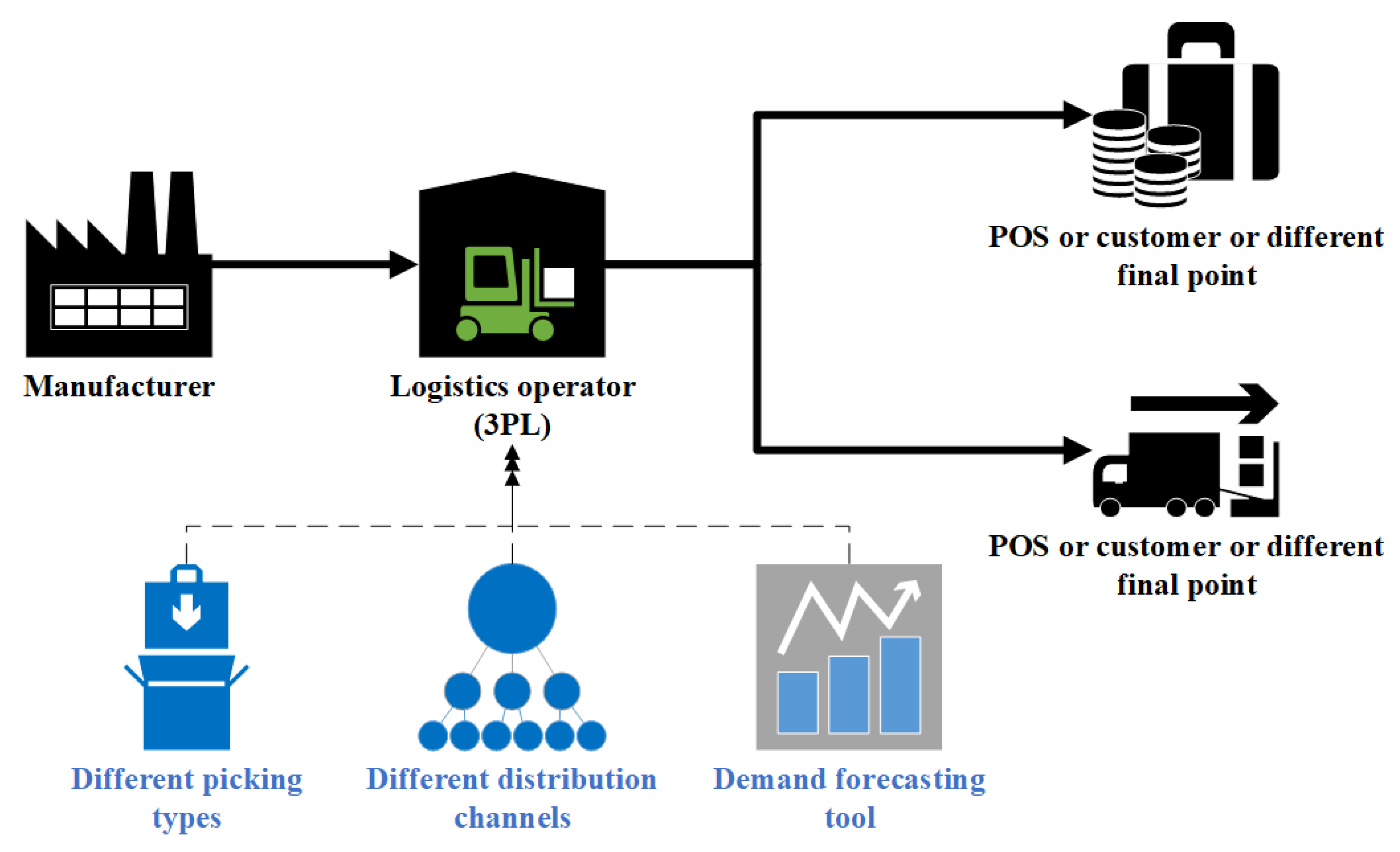
This study employs a case study approach focusing on two distribution networks where a logistics operator provides logistics services to a manufacturing enterprise (
Figure 2).
This is a logistics company specializing in providing services related to the distribution and warehousing of goods for various enterprises. The company offers a wide range of logistics services, such as transportation, warehousing, supply chain management, freight forwarding services, and inventory management. This operator continuously invests in modern technologies and trains its employees to meet market demands and enhance its competitiveness. It operates internationally, mainly in Europe, but also beyond.
As part of its operations, the operator uses a forecasting tool powered by data from the WMS (Warehouse Management System). To improve its warehousing operations, the operator decided to use the tool primarily to forecast aggregate dispatches (for all SKUs—Stock Keeping Units) for different picking methods and sales channels. Different picking methods imply variability in the engagement of warehouse resources in the process of fulfilling customer orders. The forecasting tool used by the operator is powered by WMS data and utilizes, among other things, a modified autoARIMA mechanism (
Figure 1), based on the ARIMA (Autoregressive Integrated Moving Average) model. The ARIMA model is a time series forecasting method commonly used in statistical analysis to understand data patterns over time and predict future values based on these patterns.
The forecasting tool used by the operator leverages a commercial version of the modified algorithm (
www.cloud.google.com), which enhances the capabilities of the traditional ARIMA model. It is designed to handle time series exhibiting complex patterns and includes features such as automatic detection of seasonal periods, automatic outlier detection, and the ability to manage missing values in the data. This model overcomes some of the limitations of the traditional ARIMA model by introducing additional functionalities (
Table 1).
The discussed model is used in the operations of the logistics operator and has been collecting data for approximately half a year, gathering historical data on forecasted and actual values. Forecasts in this context were created with a 30-day horizon, with daily data updates in daily granularity. The forecasted values were aligned with managerial requirements identified during the business needs analysis of the operator and were based on forecasting aggregate dispatch volumes for SKUs, for which handling during dispatch followed a similar method (forecasts for different picking methods). The research focused on analyzing two distribution networks where the logistics operator operates and serves manufacturers. In both cases, the forecasting tool operates under the previously described assumptions and is oriented toward forecasting aggregate dispatch volumes for SKUs for different picking methods.
The first case (Manufacturer 1) involves a distribution network where the manufacturer specializes in pharmaceutical production, and the operator logistically handles two main distribution channels: distribution to hospitals and distribution to pharmaceutical wholesalers. In both cases, forecasts covered three types of picking: unit picking, carton picking, and shrink-wrapped bundle picking. In the second distribution network, the logistics operator serves a manufacturer of household appliances (Manufacturer 2), for whom forecasts are created for two main distribution channels: e-commerce and brick-and-mortar stores, divided into four main picking methods (unit picking from a mezzanine, unit picking from shelves, carton picking for e-commerce, and carton picking for stores). The general characteristics of the data for each manufacturer are presented in
Table 2.
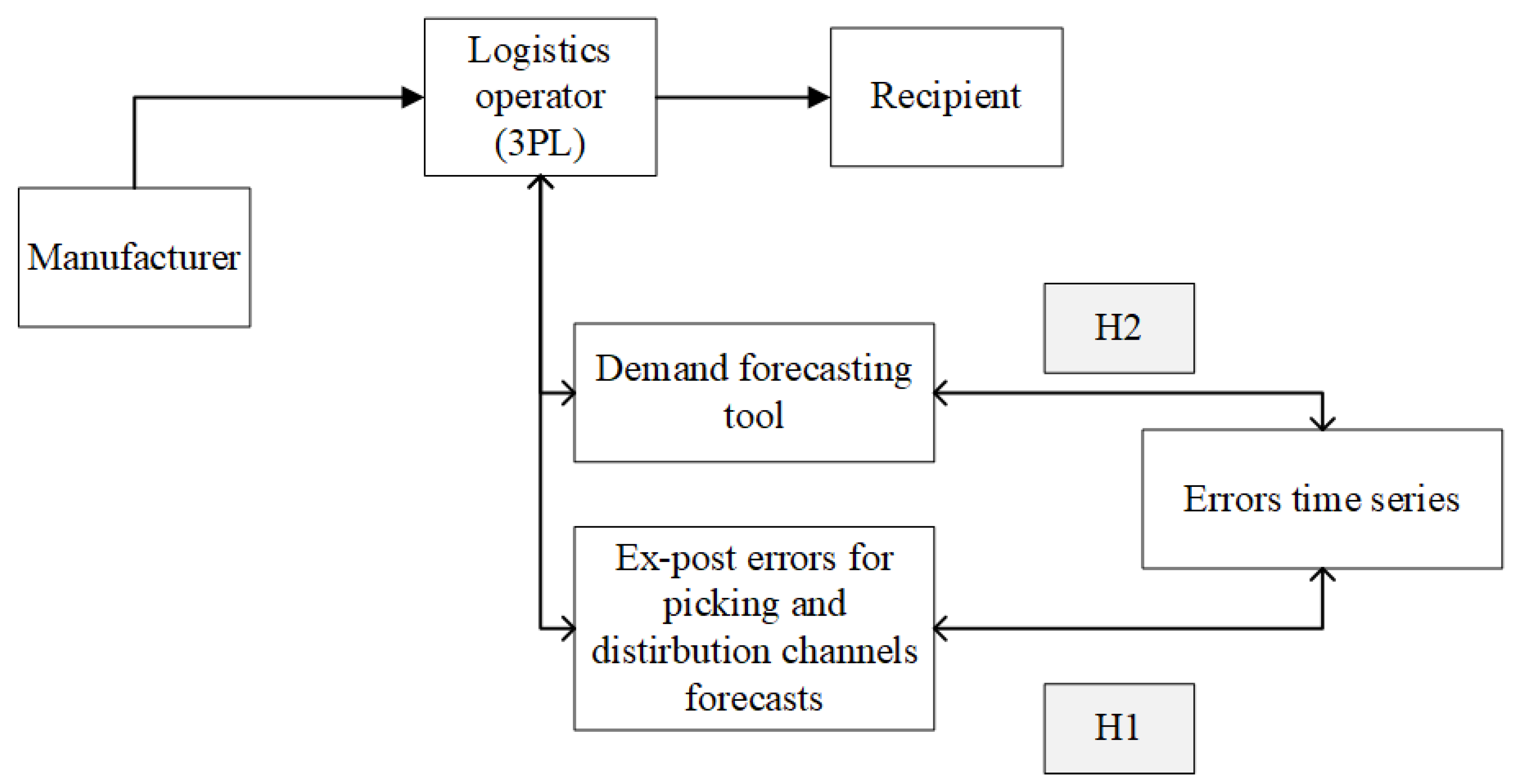
Different picking methods define varying resource consumption levels for warehouse operations related to the dispatch of SKUs in specific contexts. Accurate forecasts, therefore, improve aspects related to warehouse resource planning. The article analyzes the forecast error series collected by the forecasting tool implemented by the logistics operator. Two research hypotheses were verified in the article (
Figure 3).
The formulated hypotheses are as follows:
H1. In the forecast errors for different picking systems, certain patterns can be identified, allowing for their decomposition in terms of seasonality and trends.
H2. Analyzing the forecast error series can improve the performance of the current forecasting tool regarding the accuracy of the forecasts it generates.
The first hypothesis concerns an attempt to detect patterns, such as seasonality or deterministic components, in the forecast error series for different picking methods. Verifying this hypothesis will address whether patterns in forecast errors can be identified within the forecasting tool's operation. The second hypothesis aims to verify whether the conducted analysis can influence the tool's functionality and improve the accuracy of the forecasts it generates.
The R environment (R Core Team, 2022), specifically the "forecast" package (Hyndman et al., 2023), was used for analyzing the error series. A significance level of 0.05 was adopted for statistical inference. The "randtests" package (Caeiro F.; Mateus A.; 2022) was employed to examine the randomness of the error series. The "funtimes" package (Lyubchich V.; Gel Y.; Vishwakarma S.; 2023) was used to test hypotheses regarding the presence of trends. The "seastest" package (Ollech D.; 2021) was applied to analyze seasonality. Additionally, the procedure proposed in Wolny (2023) was used to verify hypothesis H1. Systematic components, such as seasonality and trend, were identified using STL decomposition (Cleveland et al., 1990). The strength of seasonality and trend in errors was assessed using the following metrics (Wang et al., 2006):
where
Tt is the smoothed trend component,
St is the seasonal component and
Rt is a remainder component.
Equation (3) defines the strength of the trend component, while equation (4) specifies the seasonal component. The main functionalities of the R package used for error analysis are presented in
Table 3. Detailed assumptions regarding the applied functions are outlined in the column "Functions Used." For other parameters not explicitly listed, the default values for the respective functions were used.
4. Results
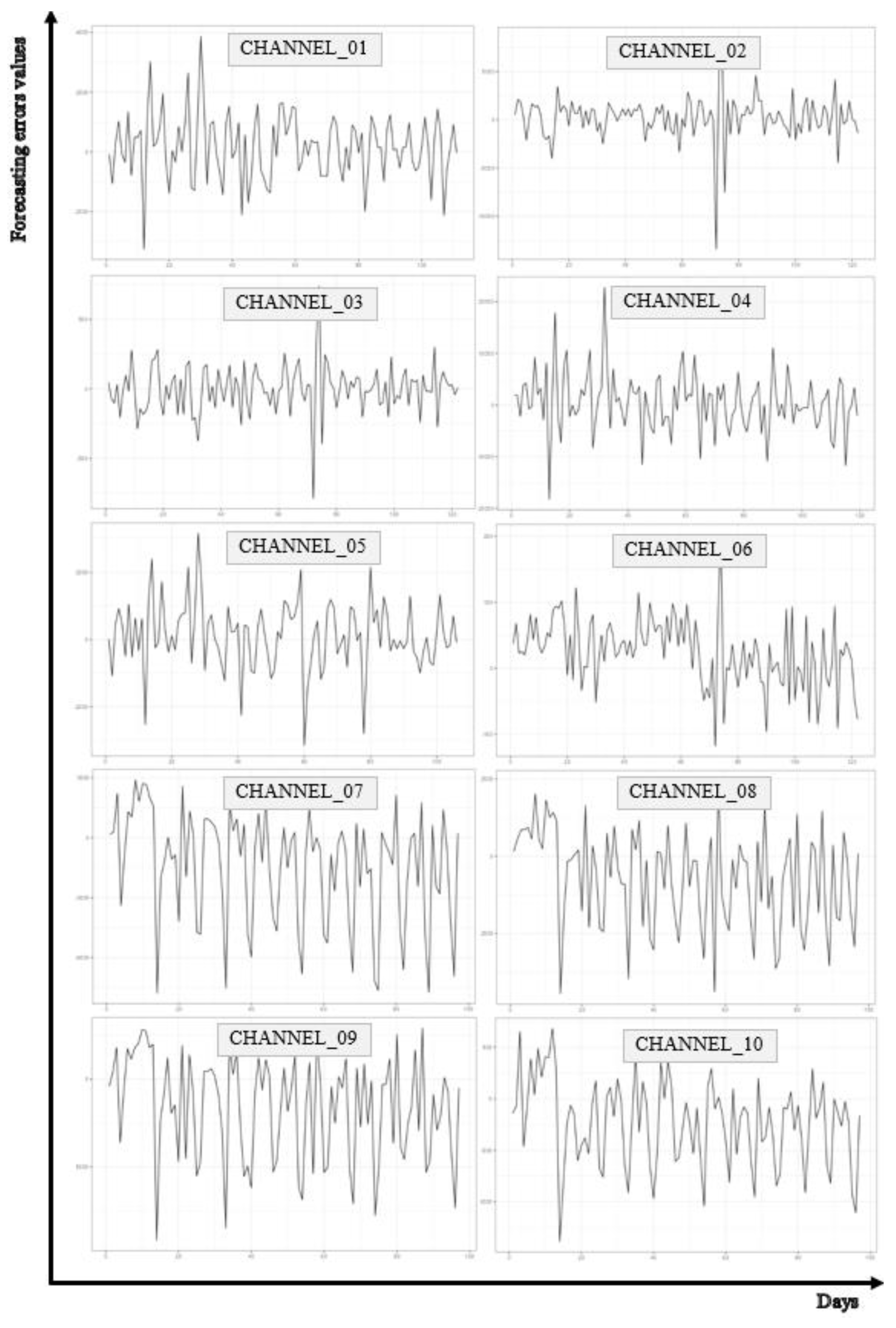
In the first step of the analysis, a visual assessment of the forecast error series was conducted. The visual analysis of time series forecast errors involves plotting these errors on a timeline. Such plots can reveal existing patterns, such as cyclicality, seasonality, or trends, which might not be evident in the analysis of the forecasted values alone. For example, if regular fluctuations are observed in the forecast error series over specific time periods, it may indicate that the forecasting model struggles to predict certain seasonal patterns. The progression of the analyzed time series is presented in
Figure 4.
The visual analysis of time series forecast errors is a crucial phase in examining forecasting models. By thoroughly understanding the patterns and properties of error series, researchers and analysts can identify significant relationships and aspects that merit further, more detailed investigation. This approach enables a deeper understanding of the dynamics of forecast errors and potential issues within the models. Following the visual analysis, it becomes possible to conduct more advanced statistical analyses. Calculating basic distribution parameters of forecast errors, such as the mean, standard deviation, or skewness, can provide insights into the characteristics and asymmetry of the errors. Furthermore, STL decomposition (Seasonal and Trend decomposition using Loess) allows for the extraction of trend, seasonality, and remainder components, which can help identify the primary sources of errors in forecasts. Statistical hypothesis testing also plays a critical role in the analysis. Determining p-values for tests under the null hypothesis of no trend or seasonality helps establish whether statistically significant deviations from these assumptions exist. The basic numerical characteristics of the analyzed forecast error time series are presented in
Table 4..
The time series analysis of forecast errors for different channels revealed diverse patterns and characteristics of errors in these channels. Some channels tend to overestimate, while others tend to underestimate forecasted values. Differences in standard deviation, coefficient of variation, skewness, and kurtosis indicate the diversity of error variability. For each channel, analyzing these parameters can provide valuable insights for further optimization and improvement of forecasting models. For Channel_01, the mean error is 176, and the median is 172, which suggests that most errors are below the mean value. However, the skewness coefficient indicates weak asymmetry in the error distribution. Nevertheless, the large standard deviation (1095) and high coefficient of variation (CV = 6.212) indicate significant error variability. For Channel_02, the mean error is 245, and the median is 507, which suggests that the models tend to underestimate predicted values. High values of standard deviation (2268) and kurtosis (11.280) indicate significant variability in the error distribution. In the case of Channel_03, the mean error is close to zero, but the low median (15.5) and large standard deviation (174) suggest that the errors have diverse characteristics. Skewness is close to zero, while kurtosis (4.387) indicates a higher concentration of values than in a normal distribution (kurtosis = 0). For Channel_04, the mean error is 574, and the median is 297, which indicates underestimation of predicted values. High values of standard deviation (5665) and kurtosis (2.270) indicate significant error variability and some degree of dispersion of the analyzed values. The distribution is positively skewed. The mean error in Channel_05 is 126, and the median is 149, which suggests slight underestimation of values. High values of standard deviation (1017) and coefficient of variation (CV = 8.040) indicate significant variability. The error distribution is negatively skewed. For Channel_06, the mean error is 25, and the median is 29.5, which suggests slight underestimation of values. Low standard deviation (52) and kurtosis (0.567) indicate relatively low variability and closeness to normality in the distribution. The error distribution is negatively skewed. The mean error for Channel_07 is negative (-1387), and the median is also negative (-687), which indicates a tendency to overestimate predicted values. High values of standard deviation (2822) and kurtosis (-0.487) indicate significant error variability and platykurtosis of the distribution. The distribution is negatively skewed. Channel_08 is characterized by a mean error of -706 and a median of -175, which suggests overestimation of predicted values. High values of standard deviation (1602) and kurtosis (-0.774) indicate some variability in errors and platykurtosis of the distribution. The distribution is negatively skewed. In the case of Channel_09, the mean error is negative (-1583), and the median is also negative (-732), which suggests overestimation of predicted values. High values of standard deviation (2969) and kurtosis (-0.726) indicate significant error variability and platykurtosis of the distribution. The distribution is negatively skewed. For Channel_10, the mean error is -228, and the median is -147, which suggests overestimation of predicted values. High values of standard deviation (420) and kurtosis (-0.354) indicate variability in errors. The distribution is negatively skewed. In general, the coefficient of variation (CV = Std.Dev / Mean) indicates high variability in the distributions of the analyzed errors.
In the next step of the analysis, the randomness of forecast errors was examined. The results are presented in
Table 5..
The analysis of the randomness of forecast errors indicates that each of the analyzed series can be considered random (in the sense of one of the applied tests and with alpha = 0.05). However, low p-value values for Channel_02, Channel_07, Channel_09, and Channel_10 in some tests may suggest the presence of certain patterns in the error progression. The stationarity analysis of the considered error series using the ADF (Augmented Dickey–Fuller test) indicates that the series can be considered stationary (p-value <= 0.01 for each series). The results of the autocorrelation analysis of the examined series are not uniform and may indicate the presence of autocorrelation. Detailed values of coefficients and critical significance levels (p-values) for the first seven lags are presented in
Table 6. The analysis utilized ACF coefficients and the Ljung-Box test.
Preliminary analyses indicate that patterns may be present in each of the considered series. In each case, autocorrelation can be observed for the first seven lags. The summary of the analysis results for the examined forecast error time series is presented in
Table 7,
Table 8 and
Table 9.
In
Table 7, the individual columns present the following information:
- “Trend_stl” – Value calculated using formula (3), indicating the strength of the trend component in STL decomposition (the closer the value is to 1, the more significant the trend component in the error).
- “Season_stl” – Value calculated using formula (4), indicating the strength of the seasonal component in STL decomposition (similarly, the closer the value is to 1, the more significant the seasonal component in the error series).
- “MAE_error” – The MAE error value (1) for a given product.
- “MAPE_error” – The MAPE error value (2) for a given product.
- “Remainder_MAE_stl” – The “non-systematic” error, understood as the MAE value of the error series calculated for the remainder component in STL decomposition (the mean of the absolute values of the remainder component of the error series), indicating the MAE error excluding systematic components of the error series.
- “Iloraz_stl” – The relative “non-systematic” error, calculated as the ratio of “Remainder_MAE_stl” to “MAE_error”, indicating what portion of the total MAE error is represented by the MAE calculated solely for the remainder component of STL decomposition.
The data in the table is arranged in non-decreasing order of the value of measure (4), which determines the strength of the seasonal component in the error series. In STL decomposition, a frequency of 7 was adopted for each analyzed series, as the operator works 7 days a week, and the data pertains to daily volumes. The results presented in
Table 7 do not reveal direct, strong, and unambiguous relationships between the listed quantities. Only the following correlations (Pearson's, alpha = 0.05) can be considered significant:
1. Between the strength of the trend component (Trend_stl) and the strength of the seasonal component (Season_stl), r = 0.59 (t = 2.426, p = 0.034). The more significant the trend component, the more significant the seasonal component.
2. Between the strength of the trend component (Trend_stl) and the relative “non-systematic” error (Iloraz_stl), r = -0.69 (t = -3.163, p = 0.009). The more significant the trend component in errors, the smaller the error associated with excluding this component.
3. Between the strength of the seasonal component (Season_stl) and the relative “non-systematic” error (Iloraz_stl), r = -0.70 (t = -3.251, p = 0.007). The more significant the seasonal component, the smaller the “non-systematic” error.
4. Between the “non-systematic” error (Remainder_MAE_stl) and the MAE error (MAE_error), r = 0.88 (t = 6.185, p < 0.001). The greater the absolute error, the greater the absolute “non-systematic” error. This relationship can generally be considered obvious.
Regarding the first point, it should be noted that in the analyzed series, the maximum value of indicator (3) is 0.158, generally indicating a weak trend component in the analyzed error series. Only in two cases is the strength of the trend component greater than the strength of the seasonal component (Channel_02, Channel_09). In the considered problem, the seasonal component of the error series is of greater importance. Particular emphasis should be placed on the numerical aspects of the method for extracting systematic components using STL. The identified trend is generally non-linear, and changes to decomposition parameters can control trend variability. At the same time, this is closely related to the seasonal component, with practically no influence on the remainder component. From this perspective, systematic components should be considered together. For predefined decomposition parameters, correlations between systematic components naturally occur. Therefore, the correlations presented in points two and three should be treated as natural. Despite the generally weak trend component, the results of trend detection using Student's t-test, Mann–Kendall test, and WAVK test (Lyubchich V. et al. 2023) indicate significant trends in most of the analyzed series. Detailed results are presented in
Table 8.
The results presented in
Table 8 indicate the presence of a trend in forecast errors for channel_02, channel_07, channel_08, and channel_09. However, based on visual assessment of the phenomenon over time, a distinct trend cannot be confirmed. To examine the presence of a significant seasonal component in the analyzed time series, the following tests were used: combined.kwr - Ollech and Webel's combined seasonality test (Ollech, D.; Webel, K.; 2020), test QS (qs.p), Friedman Rank test (fried.p), Kruskal-Wallis test (kw.p), F-Test on seasonal dummies (seasdum.p), Welch seasonality test (welch.p).
The results of the conducted tests indicate a clear presence of seasonality in the error series for channel_10, channel_07, and channel_08. For channel_09, low p-value values also suggest the possibility of significant seasonality. These results are consistent with those obtained in the analysis of the strength of the seasonal component (4).
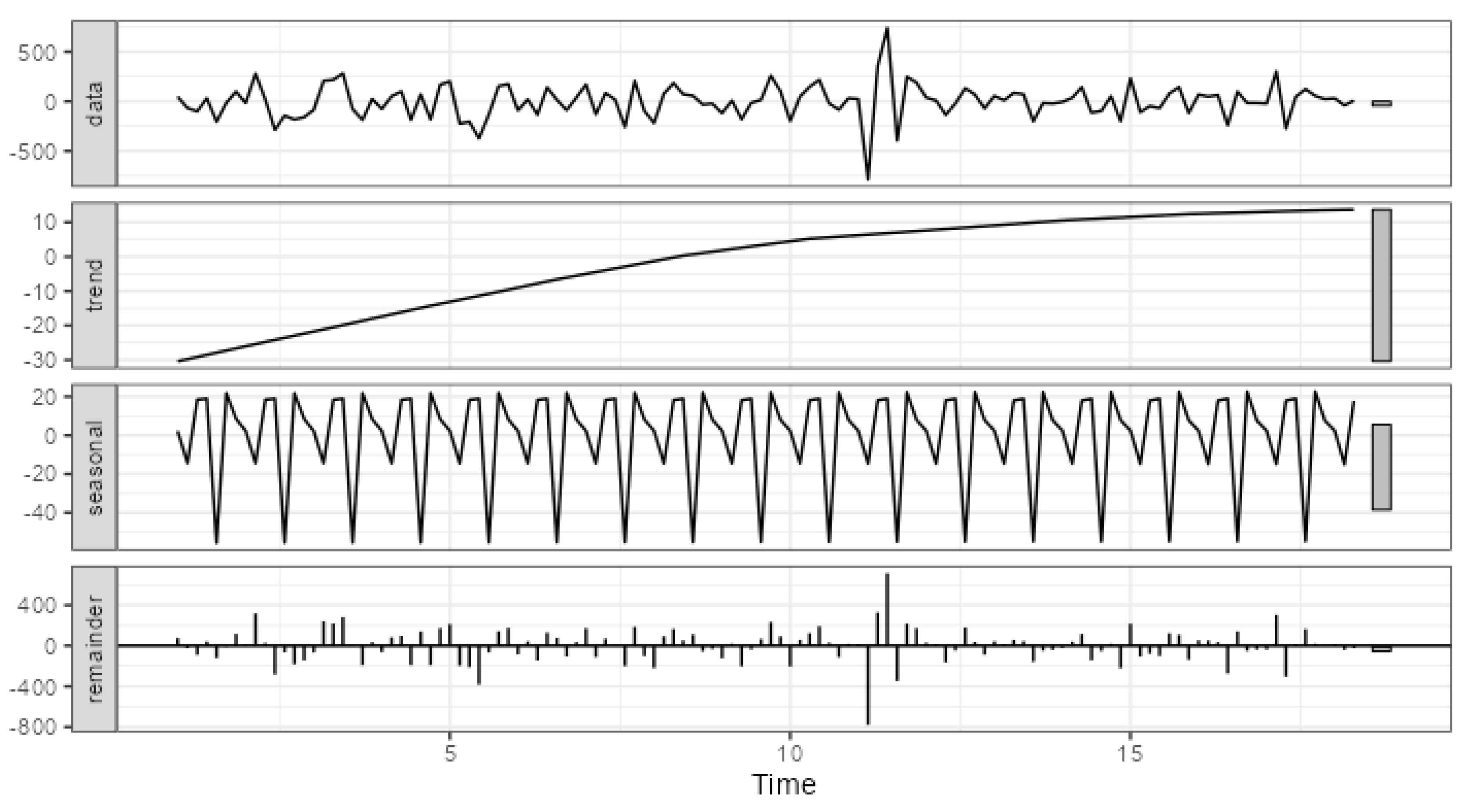
Figure 5 and
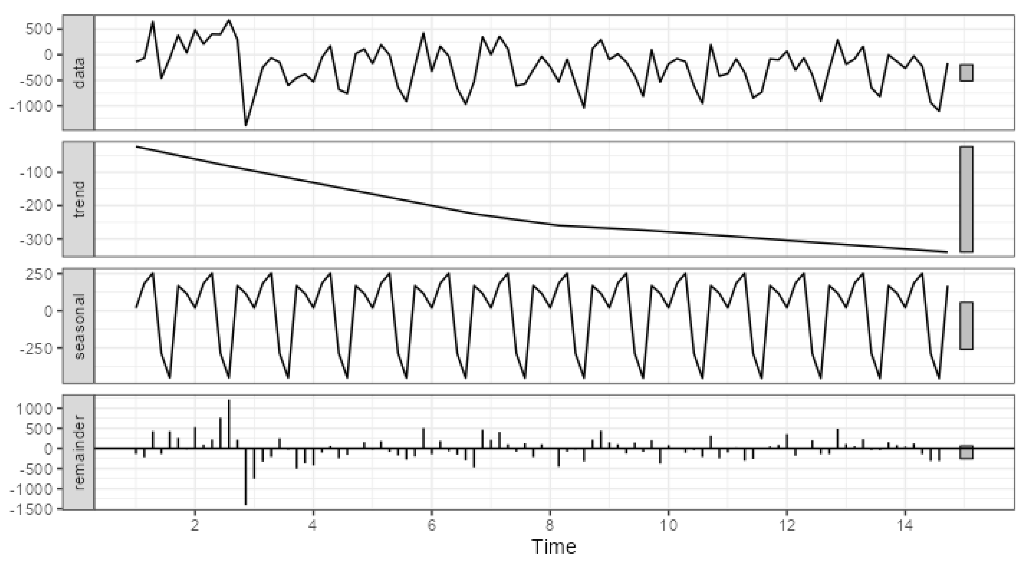
Figure 6 present visualizations of the conducted decompositions for two extreme examples.
Figure 5 shows the decomposition of errors for channel_03, which has the smallest proportion of systematic components in the total error.
Figure 6, on the other hand, presents the decomposition of errors for channel_10, which has the largest proportion of systematic components.
The primary difference in the strength of systematic components can be attributed to the scale of errors. In the case of channel_03, the trend component ranges from approximately -30 to 10, the seasonal component from approximately -56 to 23, while the range of total error variation is from -786 to 740. For channel_10, the trend component ranges from approximately -340 to -23, the seasonal component from approximately -457 to 253, and the range of total error variation is from -1388 to 681. Thus, the visualization of error decomposition can also be used to assess the strength and significance of systematic error components. It should be noted that the range of changes in individual components can serve as a key indicator in this context.
In summary, the obtained results highlight that significant systematic components in error series were identified in all examined channels of the household equipment manufacturer—significant seasonality in all channels and the absence of a significant trend only in channel 10. Regarding the distribution channels for pharmaceutical products, a significant systematic component (trend) was identified only in channel 2.
5. Discussion
5.1. Verification of Research Hypotheses
The article positively verified the first hypothesis (H1: Certain patterns can be identified in the forecast errors for different picking systems, allowing for their decomposition in terms of seasonality and trends). The analysis of forecast errors indicates that various patterns and characteristics of errors exist for individual channels. High values for the mean, standard deviation, coefficient of variation, and skewness suggest variability of errors relative to the mean. For some channels, distinct seasonal components and certain trends can be observed. The correlation values between the trend component and seasonality also suggest certain dependencies between these components. The applied analytical methods indicate consistency in the obtained results. The randomness analysis of errors showed that channels 02, 07, 09, and 10 might exhibit certain systematic patterns. The analysis of the strength of individual components in the decomposed error series also pointed to the significant importance of systematic patterns (trend or seasonality) for channel_09. In decomposition, the seasonal and trend components should be treated together, as STL decomposition largely depends on decomposition parameters (e.g., smoothing windows for trend and seasonality). The decomposition of the error series can form the basis for more in-depth analyses. In cases where significant systematic error components are present, questions arise about the causes of these patterns. Is the forecasting model failing to account for the characteristics of changes in the analyzed phenomenon, or is the systematic nature a result of some qualitative factors? Alternatively, it could prompt the search for and inclusion of an appropriate regressor previously omitted in the forecasting model.
The second hypothesis (H2: Analyzing the error series can improve the performance of the current forecasting tool in terms of forecast accuracy) was not positively verified. However, the authors suggest that there would be a high chance of its verification if detailed insights into the models used for forecasts were available or if the tool's parameters could be calibrated through simulation. The statistical test results for different channels show significant differences between groups of forecast errors in some cases (e.g., Channel_07, Channel_08, Channel_09, and Channel_10). This suggests that the forecasting tool may be more accurate for some channels than others. The presence of these differences points to the potential for improving the forecasting tool for these channels. Furthermore, the analysis of parameters such as standard deviation, coefficient of variation, or skewness helps understand how effectively the tool operates in specific cases. This could encourage a more detailed review and enhancement of the forecasting model for these specific channels. However, this was not empirically verified due to the lack of access to detailed models used for forecasting and the sensitivity of forecasted values to changes in the tool's calibration parameters.
5.2. Impact of Time Series Error Analysis on the Forecasting Tool
The logistics operator uses forecasting tools to generate predictions (Kmiecik, 2021). Time series error analysis provides essential information about the quality of these forecasts. The error values, their variability, and distribution characteristics indicate that the forecasts exhibit varying levels of accuracy and are prone to overestimation or underestimation. The forecasting tool used by the operator often generates forecasts that exceed or underestimate actual values. This suggests a need for further optimization and tuning of forecasting models to reduce forecast errors. Unfortunately, practical business tools often limit deeper analysis or modifications of their functionality. The issue of insufficient knowledge and the inability to modify such tools is frequently discussed in the literature, for example, by Voulgaris (2019) and Rahman et al. (2018). The analysis of forecast errors highlights specific areas where models encounter difficulties. Managers can focus on further refining these models by adjusting parameters, incorporating additional variables, or using more advanced forecasting techniques. Based on the analysis, a strategy for improving forecast quality can be developed. This may include designing more advanced forecasting methods, improving data collection and input management for models, and applying machine learning techniques that can better account for non-linear patterns (Ryo and Rilling, 2017; Ghosh et al., 2019).
5.3. Possibilities for Improving the Logistics Operator's Operations
The analysis of forecast error time series is critical for logistics operations. By understanding error patterns, the operator can adjust actions to better respond to forecast errors and minimize their impact on logistics activities. For example, in the case of forecast underestimations, the operator can plan for larger reserves. This is particularly important when the operator is aware that a specific algorithm does not perform well or when the data is so unpredictable or volatile that accurate forecasting becomes impossible. Understanding the characteristics of forecast errors allows for adjustments in operational strategies. For instance, when forecasting models often overestimate values, flexibility can be introduced in resource planning or storage to handle sudden demand spikes.
The analysis of different channels and error characteristics helps identify areas that are more prone to errors. Managers can implement risk management strategies, such as resource reserves or production flexibility, to minimize the negative impact of incorrect forecasts on operations. The impact of accurate forecasts on risk management by logistics operators has been described in the literature, for example, by Yoon et al. (2016) and Ben-Daya and Akram (2013). However, these authors did not consider the possibilities offered by statistical analysis of errors generated by forecasting tools. The analysis of forecast error time series is not a one-time activity. Managers should continuously monitor error characteristics, adjusting strategies as new data and experiences are gained. This allows the company to adapt its operations to changing conditions.
5.4. Main Limitations and Directions for Future Research
The analysis of forecasting errors is significant but may be limited in understanding the deeper causes of these errors. Logistics operations usually rely on many variables, which can affect forecast quality. Additionally, the lack of information about the forecasting models, calibration parameters, and input data can limit the full understanding of error sources. This lack of knowledge about models is caused by the so-called black-box effect (Rudin, 2019; Papernot et al., 2017). Efforts should therefore be made to improve the integration of the logistics operator with the provider of the forecasting software to gain a deeper understanding of its functionality. Analyzing the causes of overestimation or underestimation of forecasts can help identify specific sources of errors. Research on the impact of different forecasting models or data analysis techniques on forecast quality could lead to improved predictive results. Forecast error analysis can inspire further research on specific channels, product types, or seasonality. Innovative approaches to modeling and forecasting can improve forecast quality and enable companies to plan more precisely.