
Submitted:
04 September 2024
Posted:
10 September 2024
You are already at the latest version
Abstract
Streamflow forecasting is of great importance in water resources management and flood warnings. Machine learning techniques can be utilized to assist with river flow forecasting. By analyzing historical time series data on river flows, weather patterns, and other relevant factors, machine-learning models can learn patterns and relationships to present predictions about future river flows. In this study, an Autoregressive Integrated Moving Average (ARIMA) model is constructed to predict the monthly flows of the Athabasca River at three monitoring stations: Hinton, Athabasca, and Fort MacMurray, in Alberta, Canada. The three monitoring stations upstream, midstream, and downstream were selected to represent the different climatological regimes of the Athabasca River. Time series data were used for the model training to identify patterns and correlations using moving averages, exponential smoothing, and Holt-Winters' method. The model's forecasting was compared against the observed data. The results show that the determination coefficients were 0.99 at all three stations, indicating strong correlations. The root mean square errors (RMSEs) were 26.19 at Hinton, 61.1 at Athabasca, and 15.703 at Fort MacMurray, respectively, and the mean absolute percentage errors (MAPEs) were 0.34%, 0.44%, and 0.14%, respectively. Therefore, the ARIMA model captured the seasonality patterns and trends in the stream flows at all three stations and demonstrated a robust performance for hydrological forecasting. This provides insights and predictions for water resources management and flood warnings.
Keywords:
river flow model
; machine learning
; modeling
; and simulation
1. Introduction
Water is an essential natural resource for social development and biodiversity. However, climate change and a growing population threaten water sustainability and environmental health [1]. Particularly in a cold climate region, climate change leads to changes in river stream flows due to snow melting at its headwater and spring freshet at its downstream sections due to glacial retreat, freeze-thaw cycle, and permafrost, such as the Athabasca River in Alberta [2,4,9]. Hence, predicting stream flows is important for water resources management, flood control, and drought mitigation [3]. Generally, there are two streamflow forecasting models: data-driven models and process-based models [4] [3] [5]. Process-based models are based on physical laws representing deterministic hydrological systems and always produce the same output from a given initial state such as SWAT [6] and the WATFLOOD model [9]. However, the process-based models are highly computational and require extensive input data, such as soil types, vegetation, weather, and landscape [6]. The data-driven models use statistical analysis or Artificial Intelligence (AI) to study the characteristics of the data itself, as well as the relationship between inputs and outputs of the models, such as Genetic Algorithms (GAs), machine learning, and Artificial Neural Networks (ANNs) [7] [8] [9]. Despite the lack of hydrological process analysis, data-driven models are relatively simple and effective for streamflow forecasting. The data-driven models have often been used to predict stream flows. [10] used bagging stepwise cluster analysis to identify and group similar objects or individuals based on their characteristics or attributes. It involves a series of steps to determine the optimal number of clusters and the objects that belong to each cluster [10] and multiple subsets of the original dataset through random sampling with replacement, training a separate model on each subgroup, and then combining the predictions of these models to make a final prediction. Their results showed that the accuracy and stability of the model were improved by adding a bagging method, which is short for bootstrap aggregating when dealing with complex or noisy datasets. [11] proposed a Self-activated and Internal Attention Long-Short Term Memory (SAINA-LSTM) cell deep learning coupled with Bayesian optimization for streamflow prediction. They indicated that the SAINA-LSTM model outperforms other models in low, medium, and high flow ranges for 1- to 7-day ahead forecasts in all three highly nonlinear and non-snow-driven study basins. While the LSTMs can yield good predictions in some cases, the method still struggles with highly nonlinear time series [12,13] to analyze effectively discharge observations with different types (multiday average vs. single-day snapshot), latencies, and intervals (daily vs. weekly or monthly, etc.). [11] [14]reviewed AI-based models to predict stream flows. Their review shows that the AI-based models are still under development but have the potential to offer a more accurate and timely assessment of steam flow data availability than traditional methods. As a standard data-driven method, the Autoregressive Integrated Moving Average (ARIMA) model has been commonly used in time series analysis due to its simplicity and effectiveness [15,3] developed a multi-regime Markov-switching Generalized Autoregressive Conditional Heteroskedasticity (MS-GARCH) model (ARIMA-MS- GARCH) to predict daily streamflow with a novel multi-regime switching. Their results showed an improved prediction accuracy of the daily streamflow. These models can help mitigate risks associated with flooding, optimize water allocation, and enhance overall water resource management strategies.
Despite success predicting stream flow, developing advanced streamflow models is particularly challenging in remote/cold regions, such as the Athabasca River basin (ARB). In the ARB, changes in topography, weather conditions, and human activities, such as oil sand extraction and pulp mills, could all contribute to non-linear behaviors in river flow, leading to fluctuations in water levels, flow rates, and sediment transport. Stream flows in high latitude or subarctic regions are very sensitive to climate change due to glacial retreat, permafrost, and freeze-thaw cycle. Furthermore, data availability is generally insufficient, and record lengths are limited because streamflow and weather gauges are rare. These non-linear behaviors can make it challenging to predict and model rivers' behavior and the interconnected nature of natural systems [16]. Therefore, there is a need for hydrologic modeling and forecasting in mid- to high-latitude regions with limited accessibility [17]. To provide accurate 7-day window forecasts, a hydrological model with forecast precipitation must address the following questions: 1) Which forecasting model will produce a visualized 7-day forecast more efficiently, and how? 2) What are the limitations or challenges of this forecasting model in river /flood forecasting, especially during the ice sea? This study aims to construct a model that predicts the flow frequency of the Athabasca Rivers using a time series of river flow frequencies through the development of three models. The flood history is then compared to the correlation, which provides a context for discussion [1]. These models utilize various data sources and algorithms to simulate hydrological processes and predict future river flow levels with a certain degree of accuracy. It is challenging to predict river flow due to its non-linear behaviors, often unpredictable patterns that can occur in water movement within a river system.
2. Materials and Method
2.1. Study Area and Data Collection
The Athabasca River Basins hydrology is shifting due to increasing temperatures in the Canadian Province of Alberta, and due to climate and atmospheric factors, summer water flow has declined across the Canadian rivers; changes in water flow and water availability have impacted the ecosystem of the Athabasca River Basins ( ARB) [18]. The Mann-Kendall test, also known as the Mann-Kendall trend test, a non-parametric statistical test used to detect trends in time series data, and Sen's slope, which is widely used in trend analysis because of its simplicity and ability to handle non-linear trends, were both used to analyze the water flow of 18 hydrometric stations using data from Water Survey of Canada and data from the Alberta Environment and Parks; the results indicated that the temperatures are steadily increasing and the winter water flow is rising, the results of the study suggest that the water flow trends in the past 60 years had a decreasing trend in the middle and lower subregions, the flow rate was increasing during the cold and open warm seasons over the past 30–40 years, which is likely because of the flowrate increase in the upper Athabasca River Basins and the recent climate and land cover changes in these subregions [19]. The Athabasca River has no flow control structures that would alter natural seasonality. This provides the best opportunity to examine trends in annual flow with minimal impacts, and the results showed similar fluctuation patterns from the past historical data [20].
The Athabasca River Basin (ARB) was chosen as a case study because it is a cold climate region whose stream flow is highly vulnerable to climate change and is very important for social and environmental sustainability in Alberta province, Canada [21]. The headwaters of the Athabasca River arise from the melting snow and ice of the Athabasca Glacier, one of six significant glaciers extending from the Columbia Icefield in the Rocky Mountains near Jasper. The river flows northeast across Alberta for over 1,300 km before flowing through the Peace-Athabasca Delta into Lake Athabasca. From Lake Athabasca, water flows northward via the Slave River to Great Slave Lake, the Mackenzie River, and the Arctic Ocean. The Athabasca River is Alberta's longest river and the longest undammed river in the Canadian prairies. The Athabasca River basin covers an area of approximately 138,000 km2 and includes landscapes as varied as snow-capped mountains, agricultural plains, boreal forests, wetlands, and small urban centers [19] [22].
This study analyzed hydrometric datasets to obtain a current hydrological model of the ARB. Water flow in the Athabasca River is characterized by low winter flows followed by a rapid increase due to snowmelt in April. The Open Season or flood season is between May and August, depending on the location of the gauging station along the river. The data sets used in this research are collected from three stations, Hinton, Athabasca and Fort MacMurray on the Alberta Rivers. Figure 1 below shows the location and topography of the ARB within the provinces of Alberta and Saskatchewan and the locations of the stations [23]. The data is collected from a network of automated sensors from approximately One thousand two hundred fifty environmental monitoring stations across the province and adjacent jurisdictions following an hourly polling schedule of retrieving GOES messages and phoning stations to receive and store the station's logger data. This research will closely look at analyzing and developing the prediction model, along with an overview of the best parameters required to enhance the models for better forecasting, use quantitative data analyses, and perform linear regression analysis to evaluate the results.
The water flow data used in this study were acquired from the Alberta River Basin's website. The Alberta River Basin collects real-time hydrometric data (water flow and water level) from gauging stations across Canada. The gauging stations selected in this study were chosen based on data availability. Chosen stations had continuous data, with gaps in any parameter of no more than five years or three consecutive years in any station. Table 1 provides detailed information on each station.
2.2. Mathematic Models
2.2.1. Moving Average
The moving average, or rolling mean, is a commonly used river flow forecasting technique. It is a statistical method that calculates the average value of a series of data points over a specific period. A moving average can be applied to historical flow data to identify trends and patterns [18] [25] [15] . It is important to note that while the moving average can provide a fundamental forecast, it may not capture sudden changes or extreme events. A mean absolute error was used to calculate or plot moving average results using equation (1).
where K is the previous value, n is the number of periods, and is current observation [25].
2.2.2. Exponential Smoothing
Exponential Smoothing (ES) was first used by Brown in 1959 to analyze historical patterns and trends in the time series data; these methods can help predict future values and extend the time series beyond the existing data points. A weighted linear combination combines multiple variables or data points by assigning weights to each component and summing them together. In this method, each variable is multiplied by a weight factor, and the products are then added to obtain a single aggregated value. The weights assigned to each variable determine the importance or contribution of that variable to the overall combined value; the weight decreases exponentially with the further increase of past observations. The most negligible weight is associated with the oldest observations.
Single exponential smoothing is suitable for predicting data without clear trends or seasonal patterns. The third exponential smoothing is appropriate for the data with an apparent seasonal pattern. Due to the lack of clear trends and seasonal patterns in the observed data during equipment faults, single exponential smoothing is chosen as the basis for the algorithm [12,17]. In this research, only one parameter (flow) was considered and used to test and generate forecasting models. However, these models typically consider various factors such as precipitation, evaporation, runoff, and the physical characteristics of the river basin. More enhancements are required by inputting data on these factors; a river flow model can generate predictions of water levels, flow rates, and other hydrological parameters at different points along a river. River flow forecasting for cold regions was first developed in 1970. However, the research offers various river-flow forecasting methods that have provided some accurate results. Still, they could produce unfair results when insufficient data and (or) descriptive variables are available to describe the physical mechanisms that govern a watershed’s hydrology and misrepresent the non-stationarity of the input-output relationship. In this case, methods that can simulate the dynamics of hydrological processes and geomorphological data would be preferred because valuable information can be obtained by interconnecting such processes [22].
Exponential smoothing is a statistical method that assigns exponentially decreasing weights to past observations, with more recent data points receiving higher weights. This approach allows for capturing trends and patterns in the data while giving more importance to recent observations. Historical river flow data is typically used to apply exponential smoothing for river flow forecasting. The basic exponential smoothing formula involves calculating the forecasted value as a weighted average of the previous observation and the previous forecasted value. A smoothing factor determines the weights, often denoted as alpha (), which controls the rate at which the weights decrease. Equation (2) represents the formula for exponential smoothing.
where α is the smoothing factor of the weight coefficient, is the current Observation, and is substituted.
α is between 0 and 1. The smaller the α, the more influence the previous observations have, and the smoother the series, [25]. By adjusting the alpha , the forecaster can control the level of smoothing and responsiveness to recent changes in the data. A smaller alpha (), value results in a smoother forecast that is slower to react to recent fluctuations. In contrast, a more significant (), value makes the estimates more responsive to recent changes [25] [26]. It is important to note that while exponential smoothing can provide reasonable forecasts for river flow, it may not capture all the complexities and factors that influence river behavior.
2.2.3. Triple Exponential Smoothing “Holt-Winters”
Holt-Winters is a popular forecasting method that can be used for river forecasting. It is a time series forecasting technique that considers the trend, seasonality, and level of time series data. Holt-Winters method uses exponential smoothing to forecast future values based on historical data. In river forecasting, Holt-Winters can be applied to predict a river's future flow rates or water levels. By analyzing historical river flow data, the method can capture the underlying patterns, such as seasonal variations and long-term trends, and generate forecasts for future periods. However, it is essential to note that river forecasting is a complex task that involves multiple factors beyond just time series analysis. Holt-Winters can be a valuable tool within a broader framework of river forecasting models and techniques. It is often combined with other methods and data sources to improve the accuracy and reliability of river flow predictions. The level, trend, and seasonality can be calculated using the following equations respectfully: (3), (4), and (5). The formulas update the level, trend, and seasonality components based on the previous values and the current observation. The smoothing factors determine the weight of the current observation versus the earlier values. The forecast is then calculated by adding the level and the trend and multiplying it by the previous seasonality equation (6) [25].
where is the level at the time t, is the trend at the time t, is the seasonally adjusted value at time t, is the actual value at time t, is the seasonally adjusted value at the same season in the previous cycle, (alpha) is the smoothing factor for the level component, β (beta) is the smoothing factor for the trend component, (gamma) is the smoothing factor for the seasonality component.
3. Model Implementation
Implementing machine learning (ML), AI, and Data Mining has excellent potential to assist in developing flood forecasting systems. These systems are crucial for flood monitoring and can effectively predict flooding by extracting hidden patterns among available features of past weather data. The daily maximum water level is a parameter that can represent the level of inundation risk.
Python includes data analysis, machine learning, and visualization packages that will assist in analyzing a particular time series with data points indexed in time order [27]. For example, water flow/water level. Data will be selected or downloaded from the Alberta River Basins [24]. To assist the situation, the forecasting models should be highly accurate, predict the near future, and simulate potential hazards. Furthermore, the simulation results need to be intuitive for decision-makers and stakeholders. Therefore, the Data set will be selected and organized as follows.
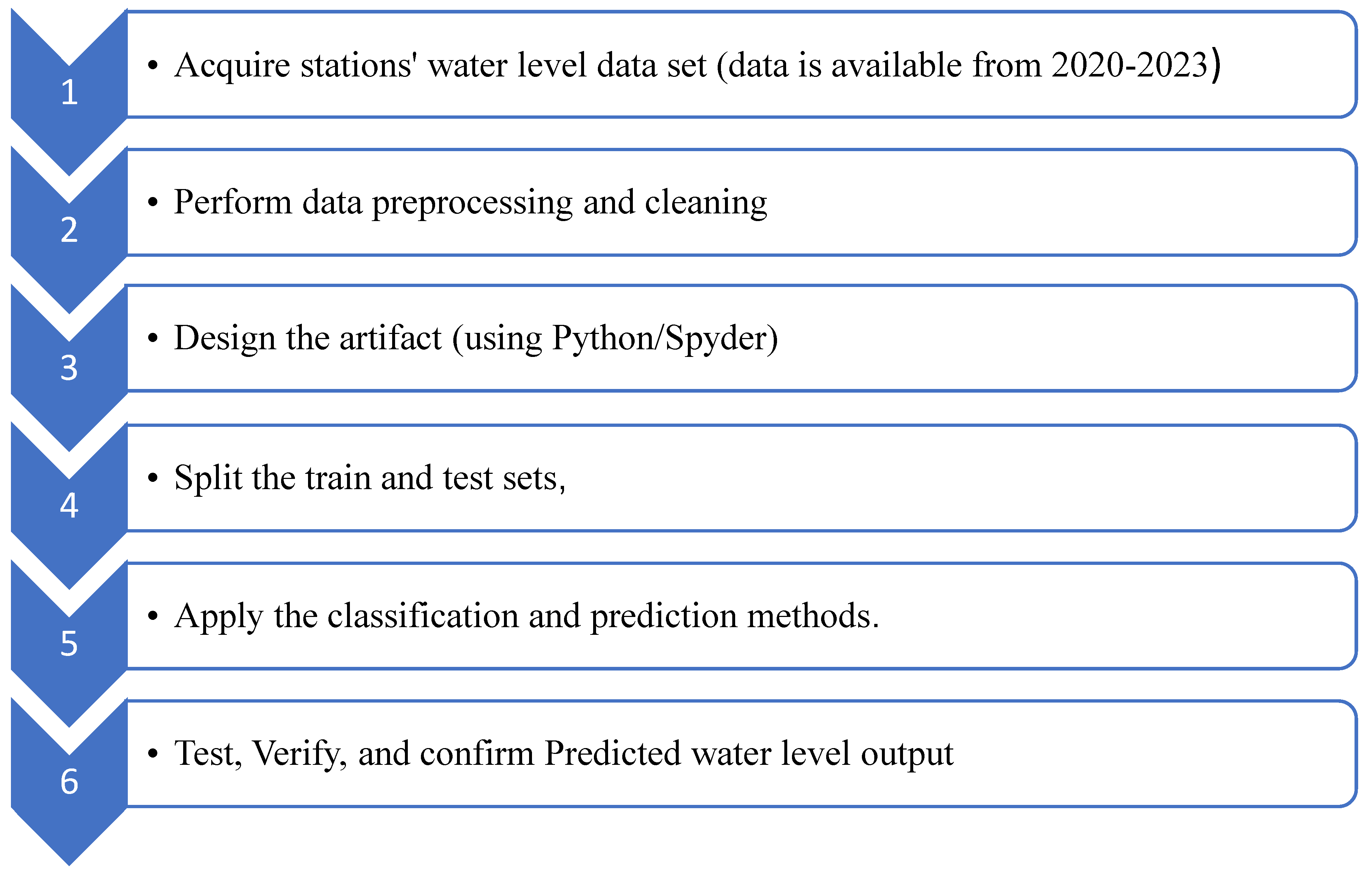
3.1. Implementation Procedure
Log in to the Alberta Basins at https://rivers.alberta.ca/, locate each station, and download each station's “Period of Extract_Q_” data.
Verify and clean the data; it needs to be consistent. Manually verify the data by opening each CSV and removing incomplete days and any duplicate or missing data for each station.
The installation steps and the code for each module are included in the Python file (Flow River Forecast), along with the linear regression technique model and the data sets, referring to https://github.com/suekamal/Flow-River-Forecast,
3.2. Statistics Performance
Sensitivity analysis can determine the accurate values of the algorithm’s parameters. Changes to the values of the parameters are communicated as the sensitivity analysis [28]. Linear regression and Bootstrap, a statistical method, were used in this research to demonstrate the relationship between a dependent variable and one or more independent variables. The modeling process effectiveness, hydrology, and climate variables are usually associated with missing data. Hence, exploring reliable methods or mathematical procedures is highly recommended to obtain where those missing data vastly influence the modeling performance. The statistics on the left represent the hourly flow, and those on the right represent the classification and regression. [29]. Table 2 provides further explanation.
- The statistics on the left represent the Hourly River Flow- Figure 5a–c.
-
Meanwhile, the statistics on the right, Figure 5a–c, represent the correlation using a forest regression to represent classification and regression [20] [14] [29].
- ○
- The scatterplot on the right visually depicts the correlation between two quantitative variables for everyone in the dataset. Each point on the graph represents a flow, with one variable plotted on the horizontal axis and the other on the vertical axis. This clear, intuitive representation swiftly comprehends the variables' interdependence [20].
- ○
- The figures on the right exemplify a blue scatterplot displaying the data from the CSV files. The measured flow (from input data or file) is displayed on the horizontal axis, and the predicted values calculated by the linear regression model are displayed on the vertical axis colored in blue [20].
- ○
- A scatterplot can provide valuable insights into the relationship between two variables.
- ○
- Statistical measures such as the coefficient of determination ("R square") are used further to assess the degree of association between the variables. Typically, a correlation coefficient greater than 0.7 indicates a strong relationship. These tools enable us to analyze the quantitative variables displayed in the scatterplot and better understand their relationship [20].
- ○
- The coefficient of determination equation (7) is based on means and standard deviations, so it is not robust to outliers; it is strongly affected by extreme observations. These parameters are sometimes called influential observations because they strongly impact the correlation coefficient [29].
- ○
- The root mean square error (RMSE) was used to evaluate the goodness of fit of the model, so it is not sensitive to outliers due to extreme observations.
4. Results and Discussion
4.1. Comparison of the Simulation Results with Observed Data
In this research, three statistical criteria were used to assess the prediction performance of the developed models. The three methods, Moving Average/Rolling mean, Exponential Smoothing, and Holt Winter's “Triple Exponential Smoothing,” provided correlation results with the expected monthly flows. This section shows the experimental setup and results of the models evaluated using a training data set for the best fit of the model that can be used for regression analysis of time series data. Tables 3,4 and 5 clearly show that a river's behavior changes over time, which affects its trends and patterns. These changes can result in fluctuations in water levels and flow rates, which vary throughout the year. In September, after the Open Water season (when snow melts and rainstorms occur), the flow at each station appears high and consistent. However, the flow gradually decreases as the weather becomes drier and colder. It is worth noting that some errors can occur in the readings/logs of the stations during November due to freezing weather (-30°C), which is typical for Canada. The tables and figures below provide the metrics obtained for the evaluation along with the abnormalities:

Table 3.
Observed Results for Station 07AD002 [25].
Table 3.
Observed Results for Station 07AD002 [25].
| Metrics | Observed Values |
|---|---|
| Time taken to build a model (seconds) | 57.40625 |
| Window | 7 |
| Mean absolute error(equation (1)) | 0.628 |
| Slen | 24 |
| Exponential Smoothing Coefficients | Alpha=0.3 Alpha= 0.05 |
| Coefficients | Alpha = 1 Beta = 1 Gamma = 1 |
| Mean Absolute Percentage Error | 0.49% |
| Regression score function | 0.9999291031812022 |
Table 4.
Observed Results for Station 07BE001 [25].
Table 4.
Observed Results for Station 07BE001 [25].
| Metrics | Observed Values |
|---|---|
| Time taken to build a model (seconds) | 733.359375 |
| Window | 7 |
| Mean absolute error (equation (1)) | 2.161 |
| Slen | 24 |
| Exponential Smoothing Coefficients | Alpha=0.3 Alpha= 0.05 |
| Coefficients | Alpha = 0.5 Beta = 0.1 Gamma = 0.1 |
| Mean Absolute Percentage Error | 2.12% |
| Regression score function | 0.9997655049450087 |
Table 5.
Observed Results for Station 07DA001 [25].
Table 5.
Observed Results for Station 07DA001 [25].
| Metrics | Observed Values |
|---|---|
| Time taken to build a model (seconds) | 589.203125 |
| Window | 7 |
| Mean absolute error (equation (1)) | 1.4302906473354215 |
| Slen | 24 |
| Exponential Smoothing Coefficients | Alpha=0.3 Alpha= 0.05 |
| Coefficients | Alpha = 1 Beta = 1 Gamma = 1 |
| Mean Absolute Percentage Error | 0.16% |
| Regression score function | 0.999 |
4.2. Simulation Results with Observed Data
Figure 3 illustrates the flow trend for each station using data from 2020 to 2023. It can be found that the model fully captured the measured data with an R2 of 0.99 at all three stations. However, the data has gaps during the initial months of each year, which can be attributed to freezing temperatures. The moving average/rolling mean indicated better results when the window was more minor. A moving average is a valuable tool for smoothing out fluctuations in data and identifying underlying trends. A window of a specific size is selected to calculate a moving average, and the average of the data points within that window is calculated. The window is then moved forward by one data point, and the process is repeated, providing a continuous, smooth representation of the data. Choosing the right window size for your data is essential, as a larger window will result in a smoother average but may lag sudden changes. A smaller window will respond more quickly but may be more susceptible to noise.
Figure 3a shows that the flow has progressively decreased over the years, with occasional spikes during severe thunderstorms. However, it can be seen that the flow decreased from 2020 to 2022 at both Athabasca and Fort McMurray, and then a big increase in 2023 (Figure 3b,c). Furthermore, the flow period increased in 2023 compared to the flow period in other years. This implies the freezing period decreased, and snow melt started earlier at the headwater. The flow increase in 2023 can be attributed to the tributaries at the middle stream (Athabasca) and downstream (Fort McMurray).
4.3. Discussion (Limitations)
This research casts light on three stations selected on the Athabasca River; the stations have historical data. However, the readings for each station were not consistent, as explained below:
Athabasca River at Hinton 07AD002. The station has historical data since 1998. The station readings fluctuate between the 5 minutes, the hour, etc. The station has readings for less than 24 hours. The station did not report any readings after January 1-2024. There are gaps in the reading for October 2022 to November 2022; the moving average, exponential smoothing, and the Holt-Winters provided results that correlate with the actual results. Figure 4(a) through 4(d)) represent the Performance of the Validated Models for Athabasca River Stations (07AD002). The Red Line Represents the predicted Flow for 2020 to 2023, using forest regression. [20] [14] [29].
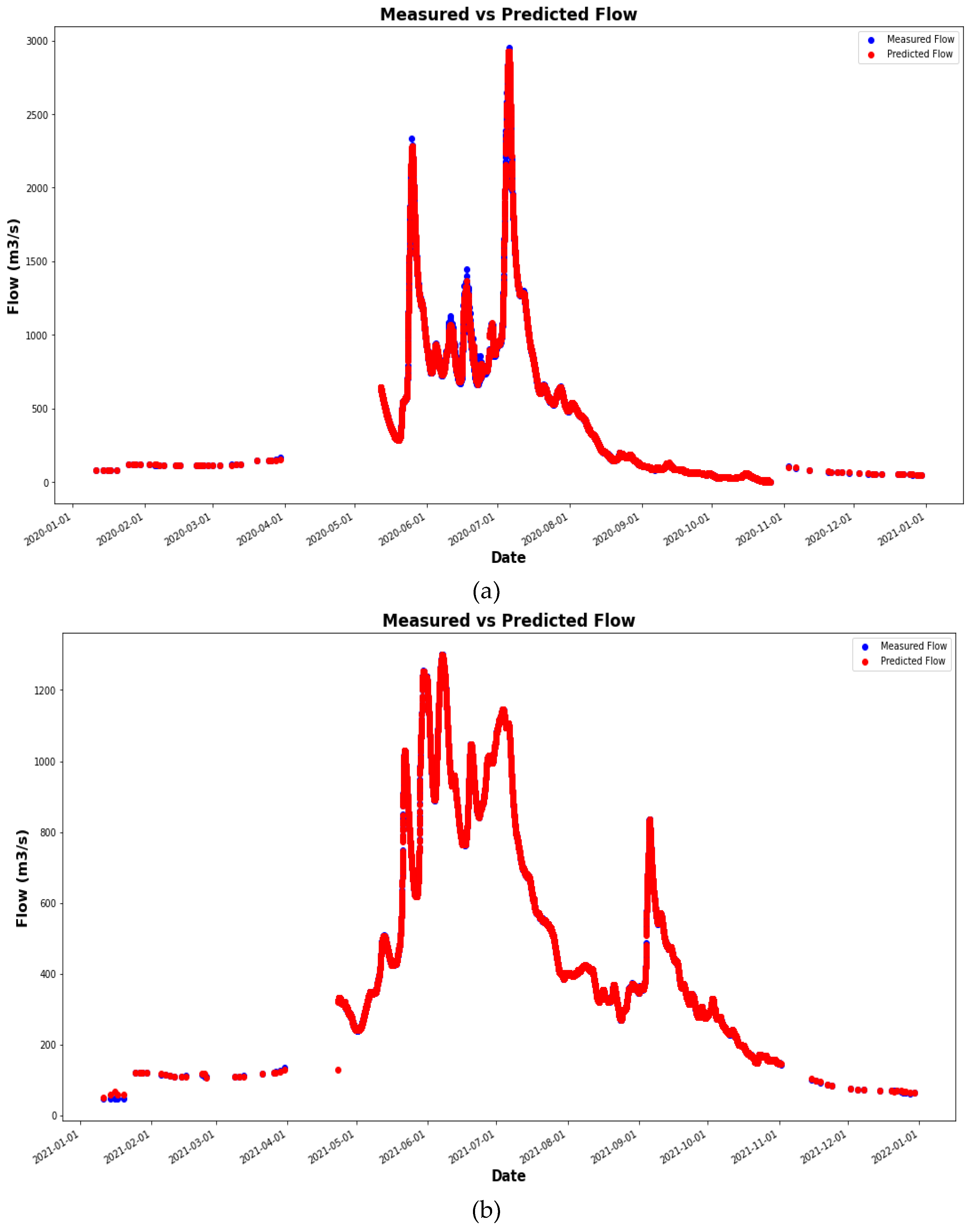
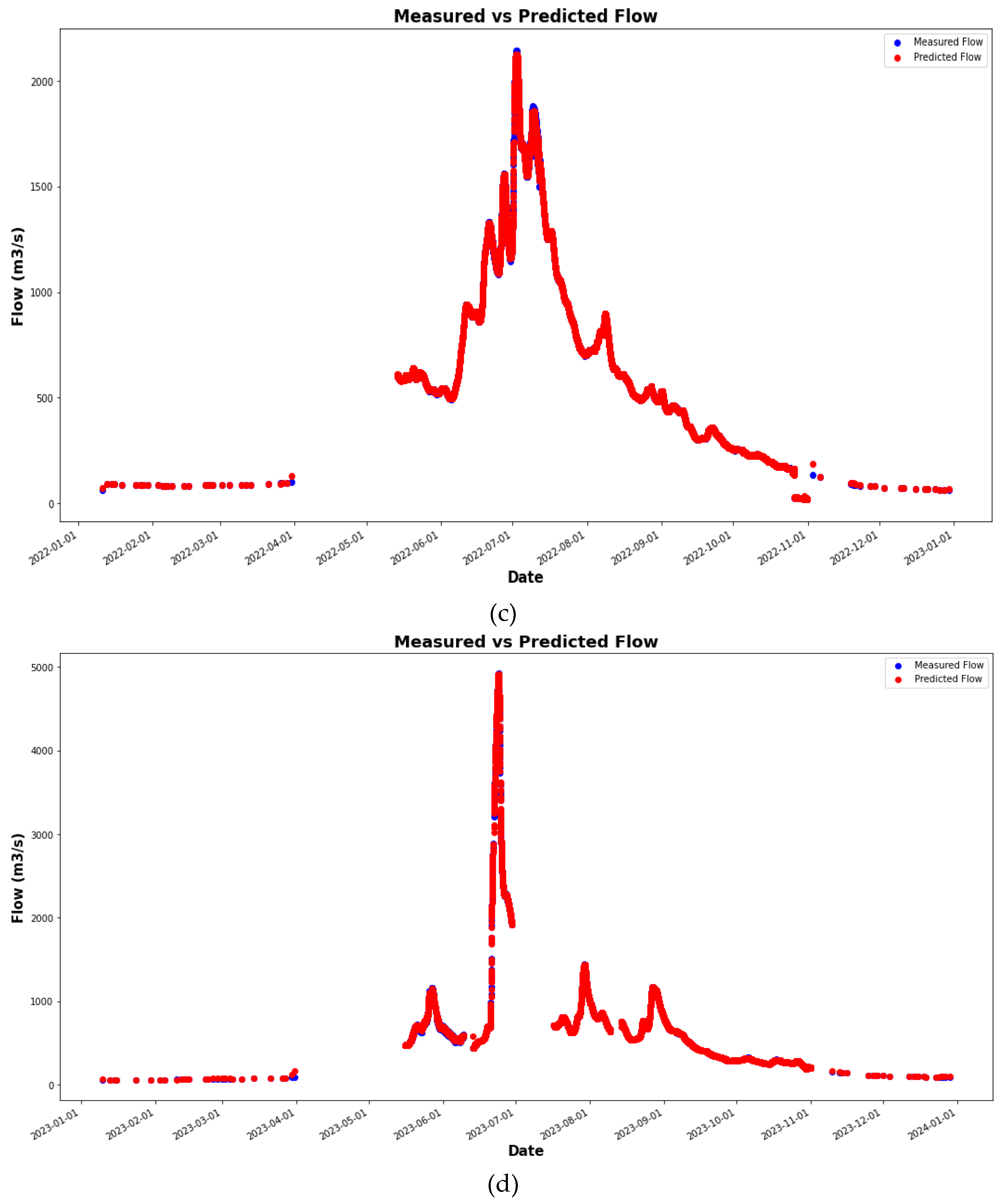
Athabasca River at Athabasca 07BE001 This station has historical data dating back to 1999. The station readings fluctuate between 5 minutes, hours, etc., and some days are reported for less than 24 hours. The station is experiencing issues with data logging, particularly during cold weather when temperatures drop below zero. This consistent problem across multiple years suggests a possible issue with the sensors or logging equipment that only occurs in freezing conditions. The three models were used or tested with the mentioned data. The moving average and the exponential smoothing models provided proper results; the Holt-Winters provided better results after adjusting the coefficients (alpha, beta, and gamma). The station did not report any readings after January 1-2024. Figure 5(a) through 5(d)) represent the Performance of the Validated Models for Athabasca River Station (07BE001). The Red Line Represents the predicted Flow for 2020 to 2023, using forest regression. [20] [14] [29].
Figure 5.
A comparison between modeled results and observed data at Athabasca (07BE001): (a) 2020, (b) 2021, (c) 2022, and (d) 2023 [10] [25] [31].
Athabasca River below Fort McMurray 07DA001 This station has historical data from 1999. The station readings fluctuated between the 5 minutes, the hour, etc., and some days had reported for less than 24 hours. The station did not report from 10:50:00 to 11:30:00. The station did not report any readings after January 1-2024. The station is experiencing issues with data logging, particularly during cold weather when temperatures drop below zero and the beginning of the springtime or ice break. This consistent problem across multiple years suggests a possible issue with the sensors or logging equipment that only occurs in freezing conditions. Figure 6(a) through 6(d) represent the Performance of the Validated Models for Athabasca River Station (07AD002). The Red Line Represents the predicted Flow for 2020 to 2023, using forest regression. [20] [14] [29].
The three models were used or tested with the four years data sets (from 2020 to 2023). The moving average and the exponential smoothing models provided proper results, while the Holt-Winters did not. The exponential smoothing method operates without the use of a window size parameter. Instead, the algorithm runs on the timestamped data series, utilizing the identified alpha values from section 4.1. Our testing employed alpha values of 0.3 and 0.05, resulting in accurate results, as in Table 3, Table 4 and Table 5.
The Holt-Winters model does not require a window size parameter; instead, it utilizes the series data, which includes timestamps and the season length, as well as alpha, beta, and gamma coefficients determined through optimization. The season length (slen), prediction timeframe (n-preds), and scaling factor (a value between 2 and 3) can all be adjusted with minimal impact on the model's performance.
It is important to note that the effectiveness of any predictive model depends on various factors such as data quality, model training, and validation techniques. Building a forecasting model can present challenges, as it requires a deep understanding of the data, underlying patterns, and appropriate techniques. Some common difficulties include selecting the correct variables, dealing with missing or noisy data, choosing the proper model, and validating its accuracy. To overcome these obstacles, having a clear objective, a well-defined methodology, and access to quality data is crucial. This research explains that using the moving average to predict the flow for a short period is acceptable. However, future predictions for more than seven days are challenging and require smoothing the original time series, understanding the trends, detecting common patterns, checking for abnormalities, using more complex formulas and algorithms, taking into consideration the importance of including the seasonality and level; adjusting the coefficients provides an optimal set of parameters suitable for predicting the flow level, which provides reliable information for enterprises to develop preventive maintenance plans.
5. Conclusions
These data sources allow the network to perform better than the base projection LSTM model. Such benefits were not simply because of the long memory of the forcings, as assimilating precipitation data did not provide any performance gain. In general, the Python models exhibit optimistic predictive models that can be utilized as a practical alternative to state-of-the-art models for river flow forecasting. The model reveals a great potential to improve the level of accuracy of the three models. The proposed Python model Holt-Winters will likely be considered a reliable forecasting tool for the inspected area. However, the Python model's behavior demonstrates a noticeable challenge in forecasting high river flow patterns due to the high fluctuations and randomness of the model input datasets [7]. The moving average/rolling mean models were tested for future prediction using various station data, and forecasting accuracy decreased as the window size increased. Exponential smoothing is valuable for analyzing trends over time and providing short-term forecasts. By prioritizing recent data points, it is especially effective at detecting short-term fluctuations and responding promptly to shifts in the data. This method is well-suited for data with a consistent pattern and can be customized to emphasize recent observations. On the other hand, Triple exponential smoothing Holt-Winters, an extension of exponential smoothing that also considers seasonality in the data, is suitable for time series data with trends and seasonal patterns, making it a powerful tool for forecasting data that exhibit both long-term trends and seasonal variations. In addition to evaluating the Python models, it is vital to consider the impact of the location of the selected stations for this test. River-flow forecasting in cold regions presents a challenge due to ice formation, snowmelt, and freezing temperatures impacting water flow. These conditions can complicate the accuracy of predictions and require specialized models and data inputs to account for this variable. Forecasting river flow in cold regions highly depends on a basin's climatic topography and geomorphology. This translates into increased model uncertainty and a substantial limitation when forecasting river flow in cold areas, often poorly gauged or ungauged. Moreover, drainage capacity decreases during the winter due to freezing temperatures, and the upper layer of the soil also tends to freeze up to a certain depth, limiting drainage capacity. Consequently, river-flow forecasting in cold regions is often challenging because a large set of descriptors in input data is required to simulate the considerable variations in seasonal patterns [30]. This research provides a significant understanding of the river flow forecasting methods, accomplishing the development of three river-flow forecasting modules, focusing on the unusual insights gained for ungauged basins in cold climates. Despite the recent progress in this field, significant challenges and limitations remain and require further research. Those include [30]:
- Limited data availability and how the stations report the data, as explained in section 4.3.
- Those models can be computationally demanding. Therefore, providing user-friendly predictive models is essential for ensuring that individuals can easily interpret and utilize the forecasts generated by AI systems.
- Designing intuitive interfaces and clear visualizations for predictive models is crucial for enabling users with varying technical expertise to interact effectively with the models. By simplifying the user experience and presenting information user-friendly, individuals without a technical background can still benefit from the insights provided by the models. This approach reduces the complexity of the models and minimizes the computational resources required for their operation. Ultimately, creating more simplistic interfaces can help lower the barriers to entry for end-users and enhance the accessibility and usability of predictive models across different domains.
- Developing a universal method for transferring regionalization parameters requires variability in catchment characteristics across different sites. Researchers can better categorize and assign regionalization parameters based on standard features shared among catchments by creating a set of classes representing watershed characteristics. This approach can help standardize the regionalization process and improve the consistency of outcomes when applying regionalization methods to diverse sites. Utilizing advanced AI techniques, such as machine learning algorithms, can assist in identifying patterns and relationships within the data to develop a more robust and transferable method for regionalization parameter transfer.
- Standardizing calibration and validation dataset selection is fundamental in ensuring the accuracy and reliability of predictive models, especially in the context of hydrology in cold climates. The choice of calibration and validation datasets can significantly impact model outcomes, and using time-dependent inputs during calibration can introduce bias. Various data-splitting methods can help achieve temporal and spatial representativeness, but specific guidelines or standards for modeling hydrology in ungauged catchments in cold climates are lacking.
In conclusion, the proposed statistical model(s) are not meant to replace comprehensive deterministic river flow models but provide a simple alternative. A more complex model is required to predict and prepare for these seasonal variations, cue temperature changes, and provide more accurate and reliable forecasts for time series data that exhibit complex patterns and variations. Future recommendations would be to validate the proposed methods in other basins and explore how different rainfall processes affect runoff production to improve the accuracy of runoff forecasting. Developing standardized protocols for dataset selection in these challenging environments is essential to improving the robustness and applicability of hydrological models in cold regions. Moreover, Hybrid models can leverage the strengths of process-based models, which rely on fundamental principles and equations to simulate the underlying physical processes governing a model and capture patterns and relationships from observed data (flow- temperature, humidity), offering a more practical and flexible approach. Integrating these two approaches creates more robust and accurate models that capture the complexities of hydrological processes in cold climates; hybrid models can be easily updated continuously with new data, informing decision-makers about choices based on current conditions and ensuring that environmental management strategies remain effective and responsive to changing circumstances. [30].
References
- J. Vörösmarty et al, "Global Water Resources: Vulnerability from Climate Change and Population Growth.," Science 289,284-288(2000). [CrossRef]
- N. K. Shrestha, X. N. K. Shrestha, X. Du and J. Wang, "Assessing climate change impacts on fresh water resources of the Athabasca River Basin, Canada," vol. Volumes 601–602, pp. Pages 425-440, December 2017. [CrossRef]
- H. Wang, S. H. Wang, S. Song, Z. Gengxi and A. O. Olusola, "Predicting daily streamflow with a novel multi-regime switching ARIMA-MS-GARCH model," pp. 47,p.101374, June 2023. [CrossRef]
- J. K. S. N. A. D. M. W. M. T. &. B. S. Wang, "Modelling Watershed and River Basin Processes in Cold Climate Regions: A Review. Water.," 2021.
- E. B. Wegayehu and F. B. Muluneh, "Short-Term Daily Univariate Streamflow Forecasting Using Deep Learning Models," vol. vol. 2022(Computational Algorithms for Climatological and Hydrological Applications):21, February 2022. [CrossRef]
- W. Junye, N. K. W. Junye, N. K. Shrestha,. M. Aghaj, T. W. Meshesha and S. N. Bhanja, "Wang, Junye, Narayan Kumar Shrestha, Mojtaba Aghajani Delavar, Tesfa Worku Meshesha and Soumendra Nath Bhanja. “Modelling Watershed and River Basin Processes in Cold Climate Regions: A Review.”," vol. Water (2021).
- X. Yu, Y. X. Yu, Y. Wang, L. Wu, G. Chen, L. Wang and H. Qin, "Comparison of support vector regression and extreme gradient boosting for decomposition-based data-driven 10-day streamflow forecasting," Journal of Hydrology, vol. Volume 582, March 2020. [CrossRef]
- J. Wang and M. A. Delavar, "Modelling phytoremediation: Concepts, methods, challenges, and perspectives.," Soil & Environmental Health (2024):, no. 100062.
- K. Taereem, T. K. Taereem, T. Yang, S. Gao, L. Zhang, Z. Ding, X. Wen, J. J. Gourley and. Y. Hong, ""Can artificial intelligence and data-driven machine learning models match or even replace process-driven hydrologic models for streamflow simulation?," : A case study of four watersheds with different hydro-climatic regions across the CONUS." Journal of Hydrology 598 (2021): 126423., 2021.
- Q. Zhang, F. Q. Zhang, F. Zhang, T. Erfani and L. Zhu, "Bagged stepwise cluster analysis for probabilistic river flow prediction," Vols. Volume 625, Part A, October 2023, 129995. [CrossRef]
- B. Alizadeh, A. G. B. Alizadeh, A. G. Bafati, H. Kamangir, Y. Zhang, D. B. Wright and K. J. Franz, "Bagged stepwise for streamflow predictin.," Journal of Hydrology, Vols. 601,126526, 2021.
- F. Liu, M. F. Liu, M. Cai, L. Wang and Y. Lu, "An Ensemble Model Based on Adaptive Noise Reducer and Over-Fitting Prevention LSTM for Multivariate Time Series Forecasting," Vols. 2169-3536, 21 February 2019. [CrossRef]
- D. Feng, K. D. Feng, K. Fang and C. Shen, "Enhancing Streamflow Forecast and Extracting InsightsUsing Long-Short Term Memory Networks With DataIntegration at Continental Scales," Water Resource Research. [CrossRef]
- H. Tao, A. H. Tao, A. Sani I, A. M. Al-Areeq, F. Tangang, S. Samantaray, A. Sahoo and H. Valadares, "Hybridized artificial intelligence models with nature-inspired algorithms for river flow modeling:," A comprehensive review, assessment, and possible future research directions." Engineering Applications of Artificial Intelligence, no. 129(2024), 107559.
- G. E. Box, G. M. G. E. Box, G. M. Jenkins, G. C. Reinsel and G. M. Ljung, Time Series Analysis:Forecasting and Control, Hoboken, New Jersey: 5th Edition, John Wiley & Sons, Inc., 2016.
- Z. M. Yaseena, S. O. Z. M. Yaseena, S. O. Sulaiman, D. C. Ravinesh and C. Kwok-Wing, "Journal of Hydrology," An enhanced extreme learning machine model for river flow forecasting:State-of-the-art, practical applications in water resource engineering area and future research direction, Received 23 August 2018. [CrossRef]
- T. L. Holmes, T. A. T. L. Holmes, T. A. Stadnyk, M. Asadzadeh and J. J. Gibson, "Variability in flow and tracer-based performance metric sensitivities reveal regional differences in dominant hydrological processes across the Athabasca River basin,," Journal of Hydrology: Regional Studies, vol. 41, no. ISSN 2214-5818, 2022. [CrossRef]
- M. Al-Juboori and A. Guven, "(2016). A stepwise model to predict monthly streamflow. Journal of Hydrology, 543, 283-292.". [CrossRef]
- Z. MS, E. Ghaderpour , H. Dastour , B. Farjad , A. Gupta , H. Eum, G. Achari and Q. Hassan , " Long Term Trend Analysis of River Flow and Climate in Northern Canada. Hydrology. 2022; 9(11):197.,". [CrossRef]
- Z. Chen and S. E. Grasby, "Reconstructing river discharge trends from climate variables and prediction of future trends,Journal of Hydrology," ISSN 0022-1694, vol. 511, pp. 267-278. [CrossRef]
- E. Ghaderpour, M. Sherif Zaghloul, H. Dastour, A. Gupta, G. Achari and Q. K. Hassan, "Least-Squares Triple Cross-Wavelet and Multivariate Regression Analyses of Climate and River Flow in the Athabasca River Basin," p. 1883–1900, 12 Oct 2023. [CrossRef]
- D. McKenney, M. Hutchinson, P. Papadopol , K. Lawrence , J. Pedlar , K. Campbell , E. Milewska , R. Hopkinson , D. Price and T. Owen , "Customized spatial climate models for North America. Bulletin of the American Meteorological Society," vol. 92(12), pp. pp.1611-1622. [CrossRef]
- E. a. Parks, "Regional Aguatics Monitoring Program," [Online]. Available online: http://www.ramp-alberta.org/ramp.aspx (accessed on 28 March 2024).
- G. o. Alberta, "Alberta River Basins," [Online]. Available online: https://rivers.alberta.ca (accessed on 28 March 2024).
- Y. Kashnitsky, "Tpoic 9.Part 1. Time sereis analysis in Python," [Online]. Available online: https://www.kaggle.com/code/kashnitsky/topic-9-part-1-time-series-analysis-in-python.
- J. Sun, J. Huang, G. Liu, R. Bai and W. Liu, "(2023). Prediction method for the truck's fault time in open-pit mines based on exponential smoothing neural network. Scientific Reports, 13(1), 18580. [CrossRef]
- Ribeiro, A. Cardoso, J. Marques and N. Simões, "2019, June. Web interface for river hydrodynamics simulation. In 2019 5th Experiment International Conference (exp. at'19)," pp. pp. 278-279.
- Ferdowsi, S. Farzin, , M. Sayed-Farhad and H. Karami, "Hybrid Bat & Particle Swarm Algorithm for optimization of labyrinth spillway based on half & quarter round crest shapes,," ISSN 0955-5986,, vol. 66, pp. Pages 209-217, 2019. [CrossRef]
- H. Tyralis, G. Papacharalampous and A. Langousis, "A Brief Review of Random Forests for Water Scientists and Practitioners and Their Recent History in Water Resources,". 2019. [CrossRef]
- D. Moore, W. I. Notz, and M. A. Fligner, Basic Practice of Statistics 6th Ed.
- Belvederesi, M. S. Zaghloul,, G. Achari, A. Gupta and Q. K. Hassan, "Modelling river flow in cold and ungauged regions: a review of the purposes, methods, and challenges," vol. Published at www.cdnsciencepub.com/er on 21 January 2022., Received 6 May 2021. Accepted 21 October 2021. 21 January. [CrossRef]
- Q. Hassan, I. Ejiagha, A. M.R, ,. A. Gupta, ,. E. Rangelova and A. Dewan, Remote sensing of the local warming Trend in Alberta, Canada during 2001–2020, and its relationship with large-scale atmospheric circulations.Remote Sens. 2021, 13, 3441. [CrossRef]
- RMA, L. Goliatt , O. Kisi , S. Trajkovic and S. Shahid , "Covariance Matrix Adaptation Evolution Strategy for Improving Machine Learning Approaches in Streamflow Prediction," Mathematics. 2022, no. 10(16):2971. [CrossRef]
- T. A. Stadnyk and T. L. Holmes, "On the value of isotope-enabled hydrological model calibration," pp. Pages 1525-1538, 2020/07/03. [CrossRef]
- Q. Zhang, F. Zhang, T. Erfani and L. Zhu, "Bagged stepwise cluster analysis for probabilistic river flow prediction,Journal of Hydrology," Volume 625, Part A,, no. ISSN 0022-1694, 2023. [CrossRef]
- P. Timoney, "New insights into the spring flood history of the lower Peace and Athabasca Rivers, Northern Canada," vol. Received 2 April 2021; Received in revised form 16 August 2021; Accepted 3 September 2021, no. 0165-232X/© 2021 Published by Elsevier B.V. [CrossRef]
- T. .. Raj , S. Shukla and . S. Sinha, "Design of Weather Forecast System Using R. Alexandra, Cardoso. Alberto , Sá Marques. José Alfeu, Simões. Nuno Eduardo," Web Interface for River Hydrodynamics Simulation, 2019 5th Experiment@ International Conference June 12th.
- X. Kang , L. Xuechun and T. Xintong , "Water Level Prediction Based on SSA-LSTM Model," vol. 2022 7th International Conference on Computational Intelligence and Applications, no. 978-1-6654-9584-4/22/, 2022.
- Z. Z. Zizi , M. Mazlina and Y. T. Hoe , "River Water Level Prediction for Flood Risk Assessment using NARX Neural Network," 2022 IEEE International Conference on Artificial Intelligence in Engineering and Technology (IICAIET), no. 978-1-6654-6837-4/22.
- T. H.F., K. M, and V. C, "Time Series Database Preprocessing for Data Mining," no. 978-1-7281-6939-2, June 2020.
- Al-Juboori and A. Guven, "A stepwise model to predict monthly streamflow," 2016. Journal homepage: www.elsevier.com/locate/jhydrol, no. Civil Engineering Department, Gaziantep University, 27310 Gaziantep, Turkey.
- M. Al-Omary, R. Aljarrah, A. Albatayneh and M. Jaradat, "A Composite Moving Average Algorithm for Predicting Energy in Solar Powered Wireless Sensor Nodes," no. 2021 18th International Multi-Conference on Systems, Signals & Devices (SSD'21), 2021 March.
- S, V. S and R. R, "A Comparative Analysis on Linear Regression and Support Vector Regression," 2016 Online International Conference on Green Engineering and Technologies (IC-GET), no. 978-1-5090-4556-3.
- Vörösmarty, P. Green, J. Salisbury and R. Lammers, "Global Water Resources: Vulnerability from Climate Change and Population Growth. Science 2000,289,284-288". [CrossRef]
- J. V. e. al, "Global Water Resources: Vulnerability from Climate Change and Population Growth," Science 289,284-288(2000). [CrossRef]
Figure 1.
The Location and Topography of the ARB Within the Provinces of Alberta and Saskatchewan and the Stations.
Figure 1.
The Location and Topography of the ARB Within the Provinces of Alberta and Saskatchewan and the Stations.
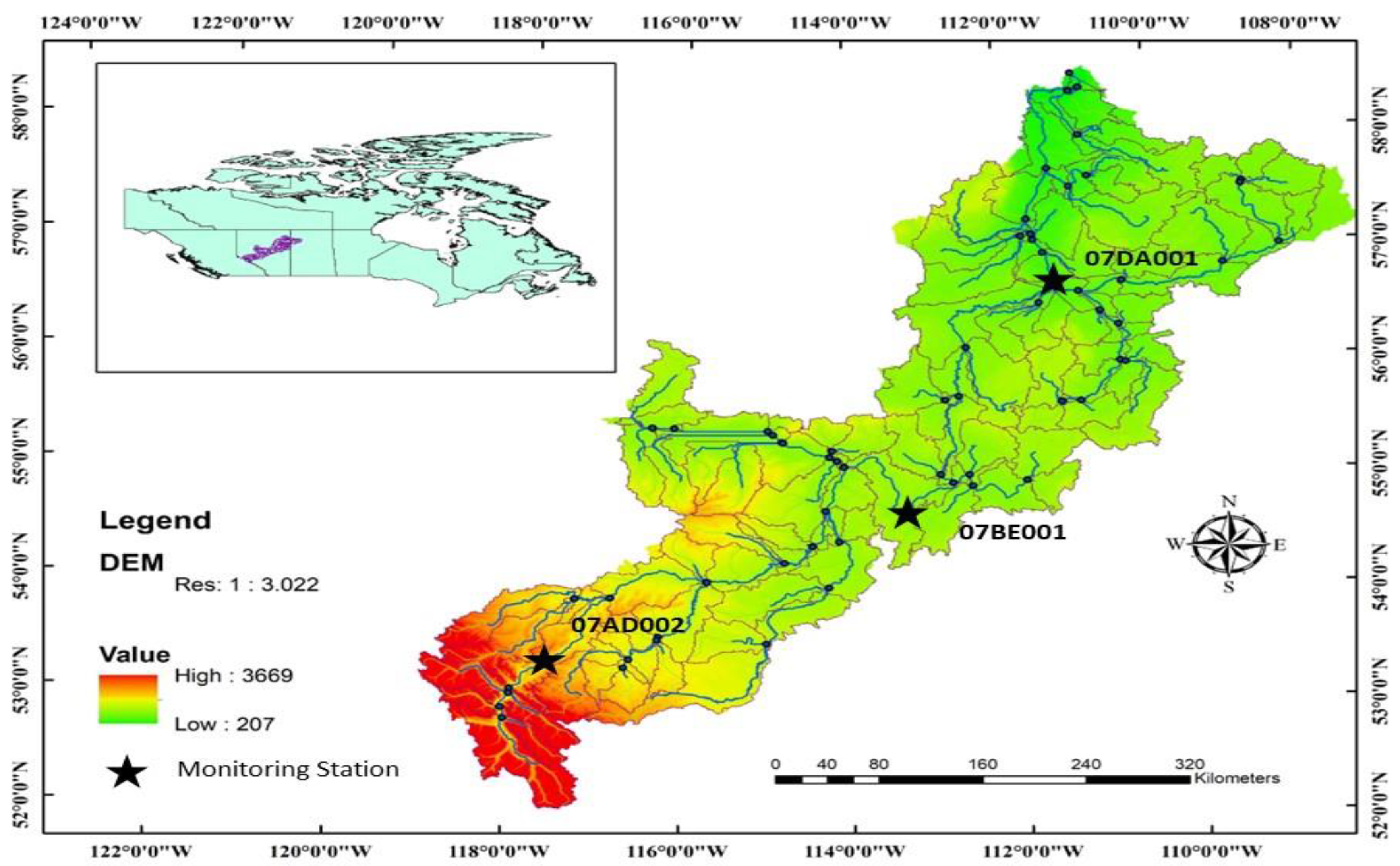
Figure 3.
The Performance of the Validated Models for Athabasca River Stations from 2020 to 2023: (a) Hinton (07AD002), (b) Athabasca (07BE001), and (c) Fort McMurray (07BE001). The Red Line Represents the predicted Flow using forest regression and blue line does is the measured data [10] [25] [31].
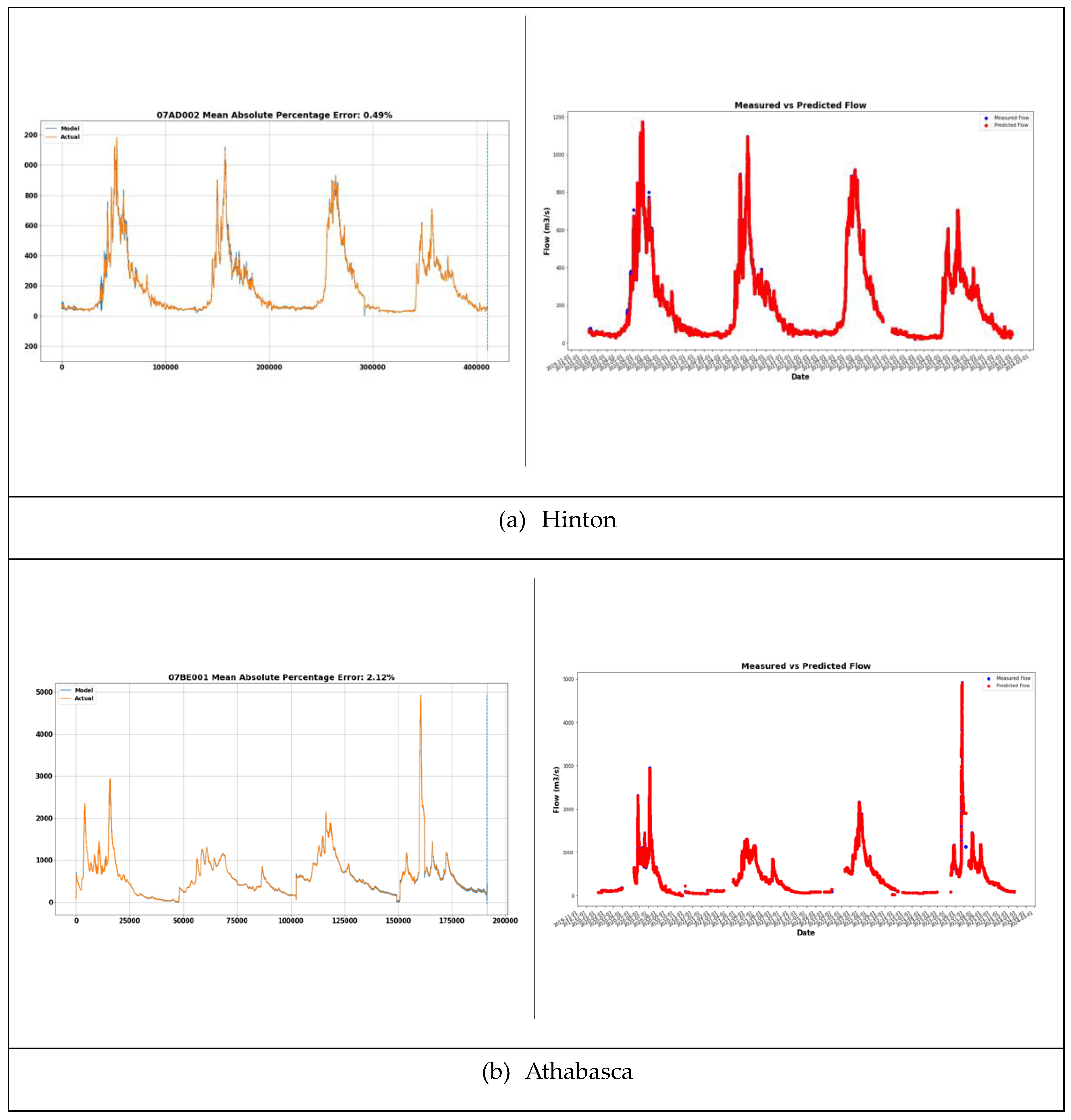
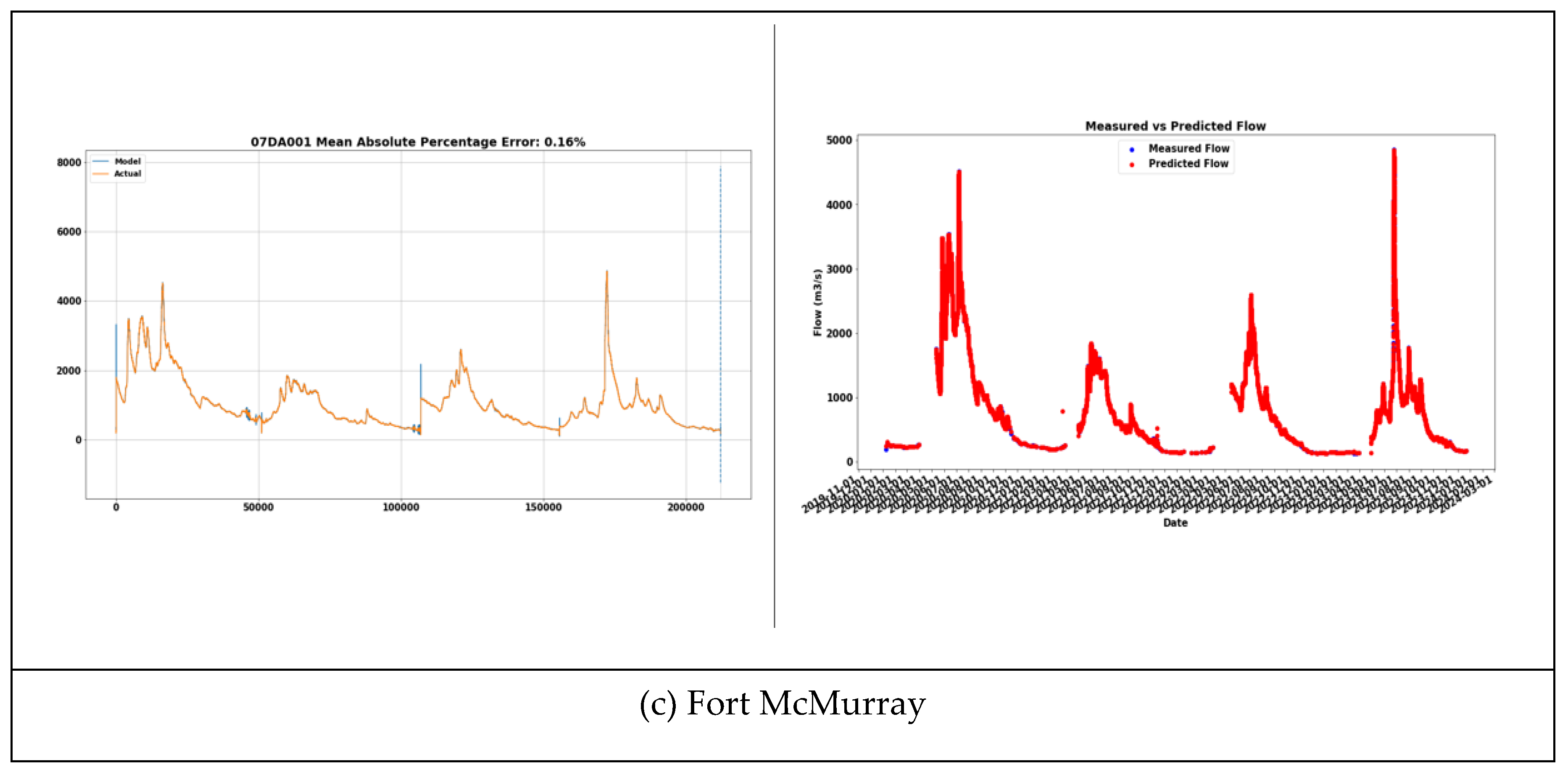
Figure 4.
A comparison between modeled results and observed data at Hinton (07AD002): (a) 2020, (b) 2021, (c) 2022, and (d) 2023 [10] [25] [31].
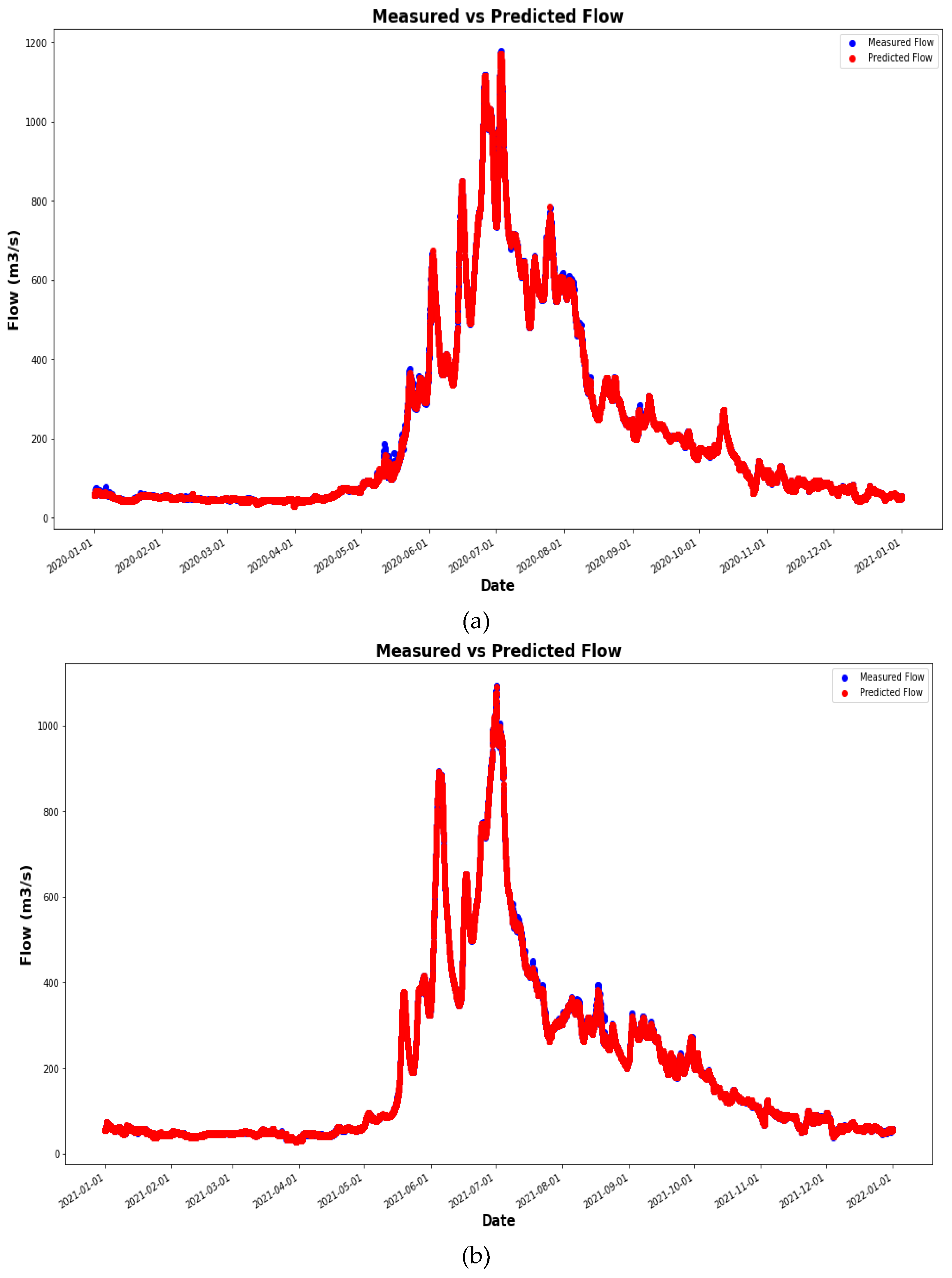
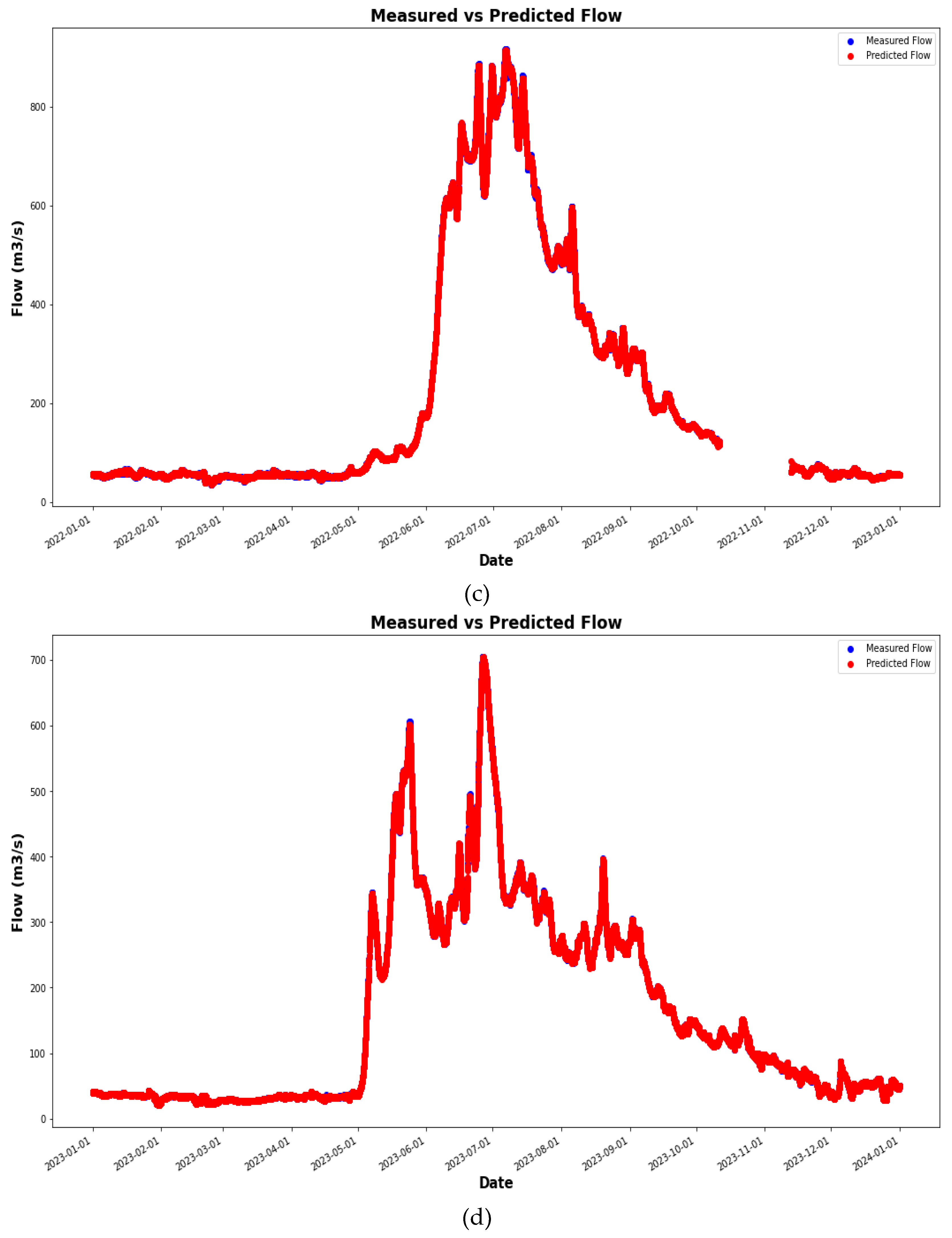
Figure 6.
A comparison between modeled results and observed data at Fort McMurray (07AD002): (a) 2020, (b) 2021, (c) 2022, and (d) 2023 [10] [25] [31].
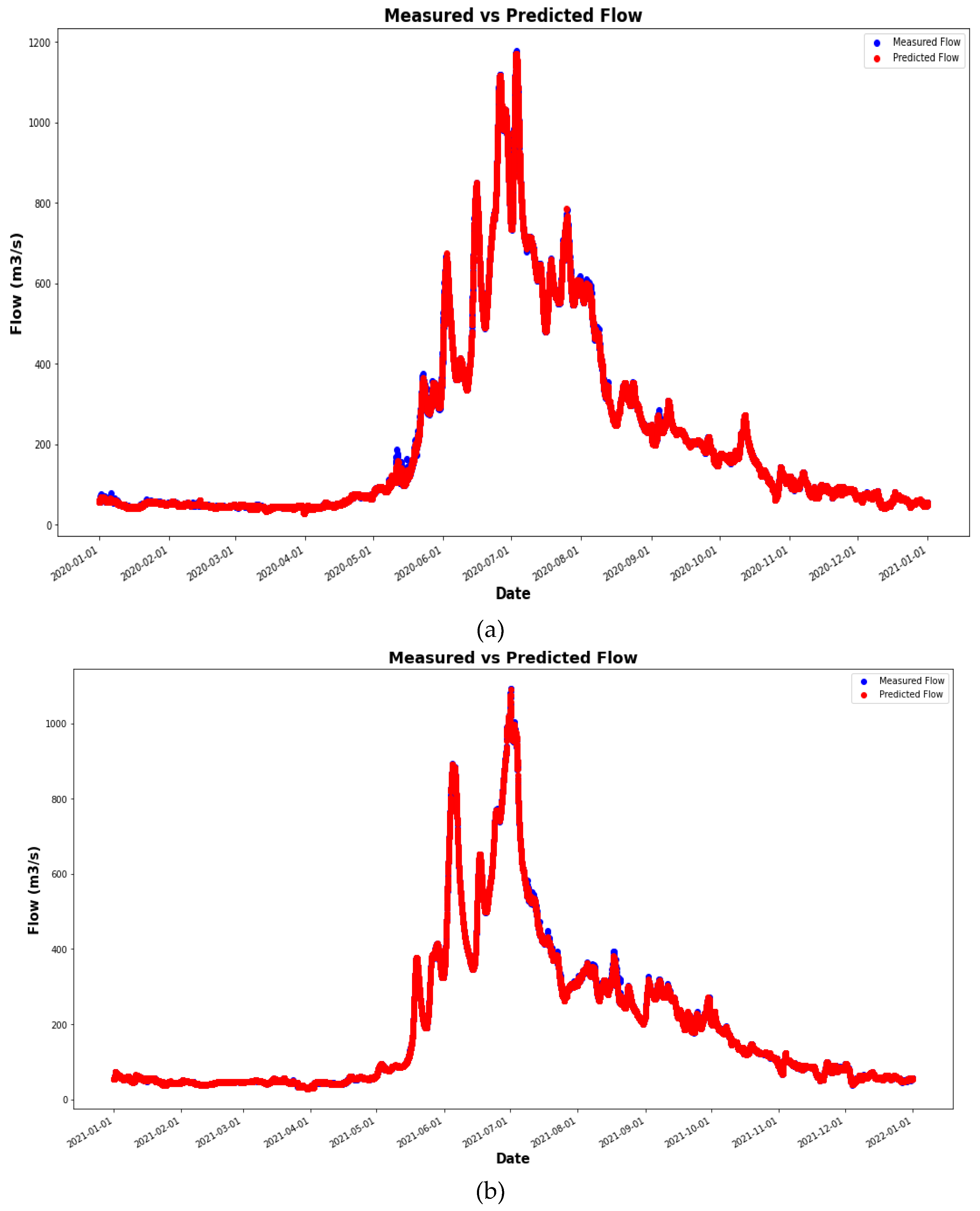
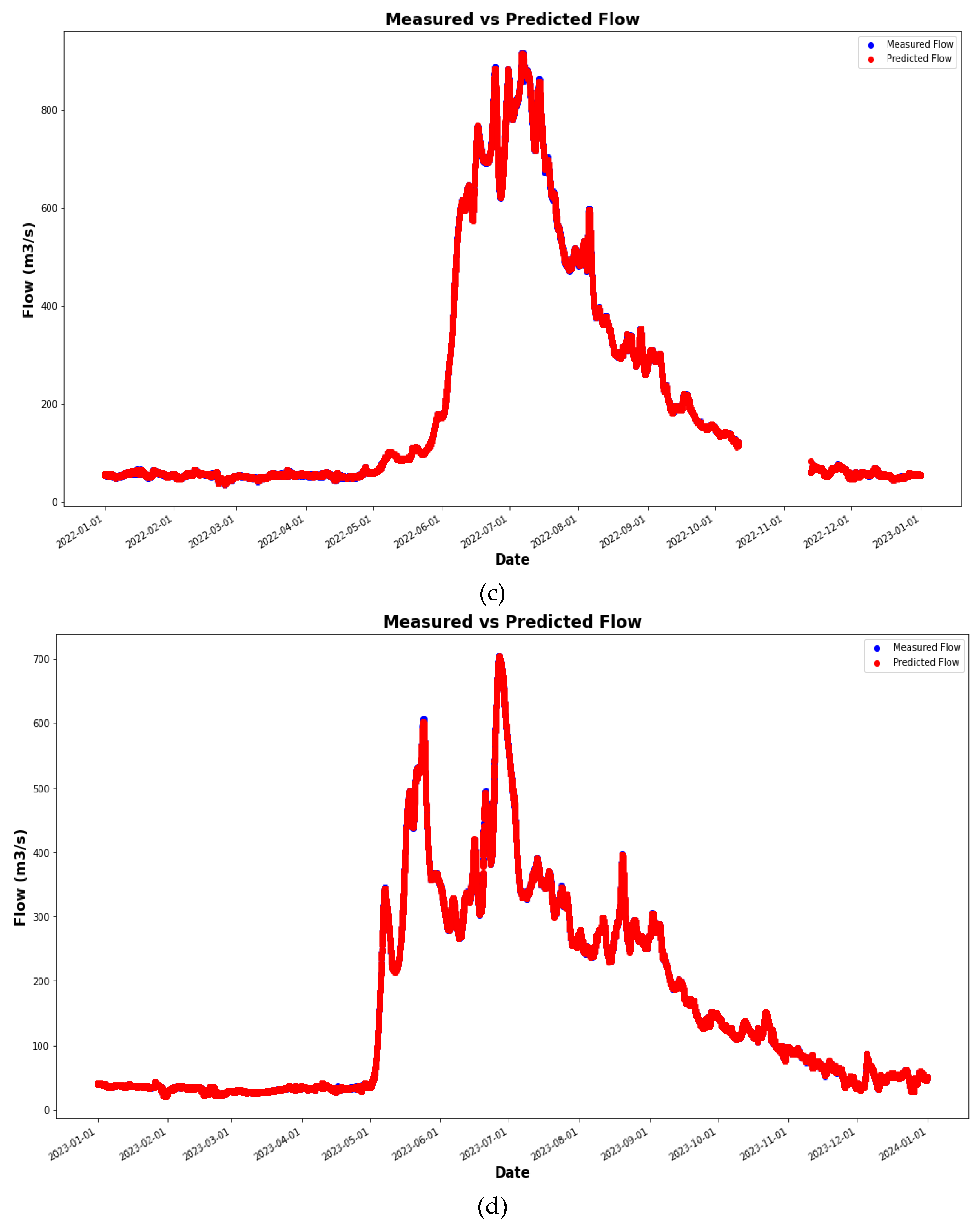
Table 1.
Description of Each Station [24].
Table 1.
Description of Each Station [24].
| Station ID | Station Name | Latitude | Longitude | Period of Records |
|---|---|---|---|---|
| 07AD002 | Hinton | 53.42429000 | -117.56942000 | 2020-2023 |
| 07BE001 | Athabasca | 54.72203000 | -113.28796000 | 2020-2023 |
| 07DA001 | Fort McMurray | 56.78035000 | -111.40219000 | 2020-2023 |
Disclaimer/Publisher’s Note: The statements, opinions and data contained in all publications are solely those of the individual author(s) and contributor(s) and not of MDPI and/or the editor(s). MDPI and/or the editor(s) disclaim responsibility for any injury to people or property resulting from any ideas, methods, instructions or products referred to in the content. |
© 2024 by the authors. Licensee MDPI, Basel, Switzerland. This article is an open access article distributed under the terms and conditions of the Creative Commons Attribution (CC BY) license (http://creativecommons.org/licenses/by/4.0/).
Copyright: This open access article is published under a Creative Commons CC BY 4.0 license, which permit the free download, distribution, and reuse, provided that the author and preprint are cited in any reuse.


