Submitted:
09 September 2024
Posted:
10 September 2024
You are already at the latest version
Abstract
This article compares the predictive capabilities of six models namely the Linear Discriminant Analysis (LDA), Logistic Regression (LR), Support Vector Machine (SVM), XGBoost, Random Forest (RF) and Deep Neural Network (DNN) to predict the default behaviour of credit card holders in Taiwan using data from the UCI machine learning database. Python programming language was used for data analysis. Statistical methods were compared with machine learning algorithms using the confusion matrix measured in metric terms of prediction accuracy, sensitivity, specificity, precision, G-mean, F1 score, ROC and AUC. The dataset contains 30,000 credit card user’s information with 6636 default observations and 23,364 non-default cases. The study results found that modern machine learning methods outperformed traditional statistical methods in terms of predictive performance measured by F1 score, G-mean and AUC. Traditional methods like logistic regression were marginally better than linear discriminant analysis and support vector machines in terms of predictive performance measured by area under the receiver operating characteristic curve. In the modern machine learning methods, deep neural networks were better in most of the predictive performance metrics than XGBoost and Random Forest methods.
Keywords:
Credit card default
; Confusion matrix
; Deep Neural Network
; Default prediction
; Linear Discriminant Analysis
; Logistic regression
; Machine learning
; Random Forest
; Support Vector Machine
; XGBoost
1. Introduction
The consumer credit in the U.S. rose by $8.93 billion in June 2024, following an upwardly revised $13.94 billion increase in the prior month, and below market expectations of a $10 billion gain (Saraiva, 2024). Also, the revolving credit, including credit cards, fell by nearly $1.7 billion, marking the largest drop since early 2021. Meanwhile, non-revolving credit, such as loans for cars and education, climbed by $10.6 billion, the highest in 2024 (Saraiva, 2024). Americans have reduced their credit card debt and even reduced their credit card spendings mainly because banks are carefully selecting the customers to extend credit (Dicon, 2024). The credit card debt default crisis took place in several countries like South Korea in 2001, and Hongkong in 2002, followed by Taiwan in the year 2005 (Chang, 2022). The same study highlighted adverse borrower selection and information asymmetry as the main reasons for default. The Taiwan cards and payments market size was $139.5 billion in 2023, and the market is expected to grow at 8% till 2027 as per the Globaldata (2023) report. Taiwan has 58.12 million credit cards in circulation as of 2023, with 37.64 million active credit cards as per the 2024 press report released by the Financial Supervisory Commission of Republic of China (Taiwan).
Loan default prediction has always been a risk management strategy for financial institutions because a minor increase in the prediction accuracy results in better risk management strategies (Hubbard, 2020). Traditionally, statistical and econometric models have been used in prediction and decision-making processes. The prediction methods are not just for the purpose of assessing the credit risk and scoring the individuals, it has wider scope from risk management strategies to optimizing the capital reserve requirements, forecasting the non-performing assets and losses, and for better recovery management strategies (Gauthier et al., 2012). Better customer profiling has always been the primary objective of banks to differentiate between clients as prompt and irregular payers. Also, a minor improvement in the prediction accuracy of loan default will result in an increased profitability of the institution. In addition, early identification of the default potential of customers will help lending organizations prevent slippage into bad loans and encourage clients to repay by enforcing recovery management strategies.
Risk profiling of customers is an important aspect of credit risk management, and it is done mainly based on the assessment of creditworthiness of the borrower that is measured in terms of the customers’ ability and willingness to repay the loan. The past track record of the borrower is also an important predictor of future payments to be made by the potential borrower (Schreiner, 2000). Hence, an analysis of customers’ probability of default based on the input parameters, and model selection and validation, with an objective to predict the default will not only help the financial institutions with better risk management strategies and decision making but also help them plan their asset portfolio and diversify accordingly.
The aim of this study is to analyze credit card users’ data from the UIC machine learning platform, which contains details of credit card clients with default and non-default data. The study evaluates a series of statistical and machine learning algorithms using six predictive models that can explain the studied event through classifiers such as: Linear Discriminant Analysis (LDA), Logistic Regression (LR), Support Vector Machines (SVM), XGboost , Random Forest (RF) and Deep Neural Networks (DNN).
2. Literature Review
A study on predicting credit defaults in Ghana among micro financial institution borrowers using binary logistic regression method found that age, income, marital status, gender, number of dependants, residential status, tenure, and the amount of loan borrowed as the significant determinants of loan repayment (Ofori et al., 2014). Consumers repayment ability can be decided by income, age, number of dependants, marital status, and expenses (DeVaney, 1999). The same study highlights that consumers psychological factors influence their willingness to repay and concluded that credit scoring models are not able to capture the details of people without a credit history (DeVaney, 1999). The same study also suggested to remove irrelevant factors and update the important factors by adding weightage to the factors according to the significance levels and increase the predictive ability of the credit scoring model. Salary determines the ability of the borrower, and it affects the repayment behaviour of the borrower (Bhandary et al., 2023b) and willingness is measured by attitude that influences repayment behaviour (Bhandary et al., 2023a).
A good predictive model not only filters the customers based on performance and reduces the credit default risk but also helps to accurately plan the economic capital requirement of the bank, ultimately increasing the profitability (DeVaney, 1999). Also, loss given default is an important parameter to determine the credit default risk. It is defined as the estimated amount that is impossible to recover from an asset in the event of a default, equationally represented as one minus recovery rate. Loss given default depends on the borrower’s ability and willingness to repay, as well as the lending institutes recovery strategies (Thomas et al., 2016). Better prediction accuracy of loss given default helps the banks accurately calculate the economic capital requirement of the bank (Bastos, 2010).
Logistic regression credit scoring model was compared with neural network model for predicting credit defaults in the Indian micro-finance industry, results show that neural network model outperforms logistic regression model in calculating the prediction accuracy and the major determinants of probability of default for the model includes income of the borrower, quantum of loan amount requested, total expense, age, family size and the length of stay at current residence (Viswanathan & Shanthi, 2017). Text mining technique from the loan application forms of an online crowdfunding platform in the U.S. was analysed using machine learning to predict potential loan defaults, and findings of the study include patterns of words written by defaulting borrowers indicative of their personality traits and personality states, that seems to disclose their true nature grounded in human behaviour (Netzer et al., 2019).
The existing credit scoring methods and predictive models using machine learning techniques are not able to evaluate student loan repayment ability and loan applicants without a credit history (Liang et al., 2019). Hence, various other input parameters must be captured to measure the borrowers credit default risk for those without a credit history. The same study consolidated and evaluated the home credit default risk and identified the important features based on the scores assigned by machine learning methods to predict repayment ability of the borrower.
Machine learning outperforms traditional prediction techniques to predict loan defaults and performs significantly well to forecast recovery rates on non-performing assets when compared with regression techniques (Bellotti et al., 2021). Also, machine learning and deep learning models have better loan default prediction accuracies when compared with statistical methods like logistic regression, and there are no restrictive assumptions on the input data, and it gives the flexibility to change the input criteria with ease (Jayadev et al., 2019).
Covariance based structural equation modelling (CB-SEM) and Partial least square structural equation modelling (PLS-SEM) are limited to estimate linear relationships only; hence it is not suited for complex non-linear relations like predicting human behaviour (Leong et al., 2013) and if the research objective is prediction, then machine learning should be preferred over CB-SEM and PLS-SEM (Chin et al., 2020). Deep neural network (DNN) is a subset of machine learning that is widely used in various fields for prediction, and it estimates linear as well as complex non-linear relations extremely well and does not require any normality assumptions to be made (Chiang et al., 2006). Hence, machine learning models are the most preferred when it comes to prediction (Chin et al., 2020; Henseler et al., 2009), but it requires theoretical background since it suffers from the ‘black box’ problem (Leong et al., 2013).
Machine learning models have emerged as a significant tool in default prediction methods mainly because of the scalability and agility in terms of its design. These models are widely used in decision making for classification, regression and clustering problems. Also, these models have been applied in a variety for fields like predicting asset pricing (S. Gu et al., 2020), option return predictions(Bali et al., 2023), stock market asset pricing (Drobetz & Otto, 2021), forecasting stock prices (Lahboub & Benali, 2024), modelling stock market volatility (Boudri & El Bouhadi, 2024), hedge fund risk management (Wang et al., 2024), bankruptcy prediction (Hamdi et al., 2024), predicting banking crisis (Puli et al., 2024), credit risk assessment (Suhadolnik et al., 2023), and predicting financial inclusion (Maehara et al., 2024). Recent studies show a broad range of machine learning applications in credit risk assessment and this study aims to predict the credit card default risk with the following research questions.
RQ1. Which model has the best predictive performance as per the confusion matrix?
RQ2. Which model has the best area under the receiver operating characteristics?
3. Materials and Methods
3.1. Linear Discriminant Analysis
Linear Discriminant Analysis (LDA) is a statistical technique to find a linear combination of features that best separates two or more classes of events. The primary goal of LDA is to project the data onto a lower-dimensional space with good class separability. The equation for Linear Discriminant Analysis (LDA) introduced by Ronald Fisher is central to dimensionality reduction and classification tasks (Fisher, 1936). The equation is given below as
where
3.2. Logistic Regression
Logistic Regression (LR) is a tool for classifying binary data and making predictions between zero and one. Logistic Regression is used to explain the relationship between a binary dependent variable and independent variables. Logistic regression is used to obtain the odds ratio in the presence of more than one explanatory variable (Sperandei, 2014). It generates the coefficients and standard errors for the significance levels of the formula used to predict the probability of event occurrence. It is represented by the equation
where is the probability, and a and b are the parameters of the model.
3.3. Support Vector Machine
Support Vector Machine (SVM) is a supervised learning model used for classification problems developed by Vapnik (1998). This technique determines the best separating hyperplane between two classes of a dataset. The mathematical formulation is expressed in terms of optimization problem and decision function (Hearst et al., 1998). The optimization problem is written as
Subject to
Where is the normal vector to hyperplane, where the are either 1 or −1, each indicating the class to which the point belongs. Each is a p dimensional real vector. The final classifier is given as
where is the sign function.
3.4. XGBoost
XGBoost is a highly scalable tree boosting machine learning algorithm. It can be scaled for big data with far less resources compared to the existing systems (Chen & Guestrin, 2016). In extreme gradient boosting (XGBoost), the objective function (loss function and regularization) at iteration t that we need to minimize is given by the following equation
where is the real label from the training data set and is the function of sum of current and previous additive trees.
3.5. Random Forest
Random forests are a combination of tree predictors proposed by (Breiman, 2001a). When performing Random Forest (RF) based on classification data, we can use Gini index or Entropy, to decide how nodes on a decision tree branch. The Gini formula is given by
This formula uses the class and probability to determine the Gini of each branch on a node, determining which of the branches is more likely to occur. Here, represents the relative frequency of the class that is observed in the dataset and c represents the number of classes.
The formula for entropy is given by
Entropy uses the probability of a certain outcome to decide on how the node should branch. Unlike the Gini index, it is mathematically intensive due to the logarithmic function used in calculation.
3.6. Deep Neural Network
Deep Neural Network Architecture
A Deep Neural Network (DNN) as shown in Figure 1 is a type of artificial neural network (ANN) that has multiple hidden layers (usually more than one) between the input and output layers. Artificial Neural Networks (ANN) first proposed by McCulloch and Pitts (1943) are broadly classified into two types based on the direction of information flow between the input and output layers. The two types are feedforward neural network (Uni-directional flow of information between the layers from input to output) and backpropagation neural network (Bi-directional flow of information between the layers) (Krenker et al., 2011). Feedforward neural networks are simpler to design and test, multilayer perceptron and radial basis function are the most popular feedforward neural networks. Multilayer perceptron’s (MLP) are limited to performing linear functions only. Hence, neurons are used for non-linear transformations. Backpropagation models are advanced, complex, and accurate for increased prediction accuracies since they iterate based on the given criteria and adjust the weights and bias accordingly (Krenker et al., 2011). The weight and bias adjustment with activation function is displayed in Figure 2. The activation functions used are tangent function, logistic function, hyperbolic tangent, rectifier function, softplus function, radial basis function, Rectified Linear Unit (ReLU), Leaky ReLU. ReLU is usually used in the hidden layers as activation functions in Deep Learning (DL) models to address the vanishing gradient problem. The network learns through an optimization algorithm known as the gradient descent. This algorithm compares the predicted output with the actual output and tunes the parameters (weights and bias) of the network through an optimization technique known as the learning rate (Hochreiter et al., 2001). Other learning functions include stochastic gradient descent and conjugate gradient descent amongst many others.
The z value is calculated as given below
where, b is the bias, w is the weight corresponding to input x, and n is the number of neurons.
3.7. Methodology
The study was analysed using python programming language. The packages Numpy and pandas were used for data analysis and interpretation. LDA, LR, SVM and RF has been performed using the scikit learn package (Géron, 2022). Extreme gradient boosting was performed using XGBoost package. The study uses Keras deep learning framework for deep neural network processing, which is a high-level API on top of Tensorflow (Géron, 2022). The DNN model structure had 4 hidden layers with rectified linear units as activation functions and repetitions of 25 epochs.
The dataset has been taken from the UCI machine learning repository that is of customers payment details with default details in Taiwan released for public usage and analysis (Yeh, 2016). The dataset contains 30,000 credit card user’s information with 6636 default observations and 23,364 non-default cases. This data set contains only numeric features with no duplicates and missing values. The dataset is imbalanced and skewed since the default and non-default cases are not exactly equal. The dataset contains the following attributes as displayed in Table 1.
Data Preprocessing
ID column was removed as it would not add value to analyse the data. Feature scaling is a crucial data pre-processing technique, and it is done to ensure that none of the variables (features) dominate the model because of their magnitude, in addition to reducing the impact of outliers, if any, present in the dataset (Zheng & Casari, 2018). The input variables are rescaled to normalize the training data. Feature scaling was performed using the standard scaler in python. The dataset is split in the ratio of 80:20 for training and testing correspondingly. Furthermore, Cross validation was conducted, that is a resampling procedure to prevent overfitting and to check the model’s ability to perform well on new and unseen data. K-fold cross validation was performed to prevent overfitting of the model and to avoid normalizing the outliers, and it was done in 10-folds as it is the widely used (Nti et al., 2021). The models have been validated using k-fold cross validation technique to minimize the effect of outliers, and therefore to prevent overfitting.
4. Results
4.1. Descriptives
Dataset was skewed for Limit Balance and Age as shown in Figure 3. The dataset has a greater number of clients having a limiting balance between 0 to 200000 currencies as limit balance and a greater number of clients in the age bracket of 20 to 40, i.e., clients from mostly young age to middle-aged groups. The dataset is analyzed with the most widely used metric for classifier evaluation i.e., accuracy, in addition to accuracy the study uses the model assessment method over imbalanced datasets as mentioned by Bekkar et al. (2013).
4.2. Heatmap
Heatmaps reveal complex patterns and correlations in the dataset (Z. Gu et al., 2016). The heatmap for the explanatory variables is represented in Figure 4. High correlation can be seen between the bill amounts (month wise) and the payment amounts (month wise). It is not an issue since it is expected to be high. It means that it is highly likely that a person spending a certain amount in the month of April will do so in the coming months also. Similarly, the person who makes a certain payment in the month of April will do so in the coming months also. The pair-wise correlation values indicate that the explanatory variables are range-bound, and they do not display strong interdependence. It is an indication that the explanatory variables are independent of each other and display sufficient divergence to be treated as separate variables for further analysis.
The Figure 5. Shows the relationship between the bill amount generated (Y-axis) and the corresponding payment made (X-axis) month wise for 6 months. Since maximum number of datapoints along the Y-axis are tightly packed near the scale zero of X-axis in all the 6 plots, it can be inferred that there is greater proportion of clients for whom the bill amount is high, and at the same time the payment done against the bill amount is very low. This indicates that the dataset contains significant details about delayed payment or default cases every month.
4.3. Confusion Matrix Analysis
The data is analysed as per the confusion matrix in Table 2 and the metrics mentioned in Table 3. The confusion matrix for the various models are mentioned in Table 4 and the metrics for the various models are given in Table 5. The prediction accuracy of deep neural network was at 81.80% that is better than all the other models. The accuracy of the modern methods like XGBoost, RF and DNN, was marginally better than the traditional models like LDA, LR and SVM. The modern methods performed well in predicting the sensitivity, but the traditional methods were better in terms of specificity. The precision score of 0.7047 for the SVM model was better in comparison to all other models. The F1-Score of DNN at 0.4820 was the best in comparison to other models and the modern methods outperformed the traditional methods in terms of F1-Score. Also, The G-mean of DNN at 0.6027 was the best when compared to other models and the modern methods outperformed the traditional methods in terms of G-mean score also.
4.4. Receiver Operating Characteristics (ROC)
The ROC curve illustrates the classification ability of a binary classifier system as its discrimination threshold level is varied. It is plotted with sensitivity in the Y-axis and specificity in the X-axis (Bewick et al., 2004). A good predictive model will have a ROC curve that is close to the top left corner, indicating a high true positive rate with a low false positive rate. The ROC curves for the various models are plotted in the Figure 6. Area under the ROC curve (AUC) measures the area underneath the ROC curve (Bewick et al., 2004). Higher value of AUC is desirable and a value close to 1 is considered as ideal. The area under the ROC curve was highest for the DNN model and XGBoost model at 77% and the AUC was 72% for LDA, 73% for LR, 71% for SVM, and 76% for RF.
4.5. Features Importance
Feature importance permits the researcher to peek inside the black box of machine algorithms to see which features are critical in informing a good prediction as per the ranking (Musolf et al., 2022). The feature importance for the DNN model is depicted in Figure 7. BillSum (Bill amount) emerged as the most importance feature followed by Age, Pay amount for various months, limit balance and the PaySum (Pay amount). Sex, Marital status and education attainment level were the least important features in predicting default behaviour of the borrower.
5. Discussions and Implications
The study results are discussed with previous research findings in this section. The results of this study indicate the superiority of deep neural networks when compared to all other models. The linear models like discriminant analysis and logistic regression have also shown satisfactory predictive performance. In a few cases the machine learning methods are marginally better than statistical methods and in many other metrics, machine learning methods are superior compared to statistical methods.
Hamdi et al. (2024) compared the predictive performance of Six models namely linear discriminant analysis, logistic regression, decision trees, support vector machines, random forest and deep neural network for bankruptcy prediction of Tunisian companies and found that deep neural network performed with better accuracy, F1 Score and area under the curve in comparison with conventional models. A study on predicting banking crisis in India using statistical methods like logistic regression, artificial intelligence and machine learning methods like random forest, naïve bayes, gradient boosting, support vector machines, neural networks, K-nearest neighbours, and decision trees found that neural networks and random forest models as effective models in banking crisis prediction (Puli et al., 2024).
A study on financial risk assessment using big data analysis and ten algorithms found that ensemble models using boosting algorithms outperformed traditional models like logistic regression and decision trees in terms of prediction accuracy (Suhadolnik et al., 2023). The study on predicting financial inclusion in Peru using machine learning methods like decision trees, random forests, artificial neural networks, XGBoost, and support vector machines found that these methods can be a valuable complement to standard models like generalized linear models and logistic regression models for assessing financial inclusion in Peru (Maehara et al., 2024). The study also found that neural network was the most effective method to predict account access. For account usage prediction, random forest method and support vector machines employing the radial basis function were the most effective prediction methods.
Neural network models were used to predict stock market index (S&P 500) using regression methodology with root mean square error and mean absolute percentage error and found that gated recurring unit and convolutional neural network models performed significantly well (Chahuán-Jiménez, 2024). The same study suggested the potential of combining different metrics for neural networks to improve the accuracy for decision making. The study by Lahboub and Benali (2024) found that long short term method of neural network modelling was effective when compared to auto regressive integrated moving average method in predicting the stock prices of credit companies in Morocco. Also, deep neural network models are significantly advanced when compared to conventional models in capturing complex pattern in financial time series data, and therefore have better precision in risk assessments (Wang et al., 2024). On the contrary, the study by Boudri and El Bouhadi (2024) found that simpler models like generalized auto regressive conditional heteroskedastic method outperformed complex models in neural networks like long short term memory and opined that simpler models may offer precise results and there is no need to apply complex models always for analysis.
Traditional methods like discriminant analysis and logistic regressions can capture linear relationships only and this becomes a major limitation for big data analysis. Whereas machine learning models can predict complex linear and nonlinear relationships (Chiang et al., 2006). Decision trees, support vector machines and deep neural networks are more effective to capture complex nonlinear relationships than simple linear models (Varian, 2014). Also, relying exclusively on statistical models for decision making may lead to questionable findings. Hence, it is recommended to use a wide range of tools for reaching conclusions on data (Breiman, 2001b).
Fintech companies can reduce the cost of lending by taking full advantage of the advancement in digital technology and big data analytics using machine learning methods (Bazarbash, 2019). The main advantage of using machine learning over traditional methods is the improvement in calculating the out of sample prediction accuracy but at the same time these methods suffer with a black box problem without a proper logic on the decision arrived (Bazarbash, 2019). Hence, feature importance tries to solve the black box problem by ranking the input parameters according to their importance in prediction (Musolf et al., 2022).
6. Conclusions
The main objective of this study was to compare the prediction accuracy of credit card default behaviour using traditional and modern methods. Traditional methods like discriminant analysis, logistic regression and support vector machine were compared with modern methods like XGboost, random forest and deep neural network methods. As pert the results of this study modern machine learning methods outperformed traditional statistical methods in terms of predictive performance measured by F1 score, G-mean and AUC. Also, machine learning methods performed marginally better in terms of prediction accuracy. In the traditional methods, logistic regression was slightly better than linear discriminant analysis and support vector machines in terms of predictive performance measured by area under the receiver operating characteristic curve. In the modern machine learning methods, deep neural networks were overall better than XGBoost and random forest methods.
The study focussed on credit card default prediction using various models and the findings of this study supports the findings of many other articles that confirm the superiority of machine learning models in terms of predictive performance in comparison with the traditional methods. Even though the study incorporates random forest, XGBoost and deep Neural Network, it falls short on an extensive and comprehensive comparison with other gradient boosting algorithms and long short term memory neural network methods. The comparison could have also studied the regression methods for various models with the calculated error in terms of root mean square error and mean absolute percentage error. Also, comparison with econometric methods like auto regressive integrated moving average could have added more insights to this study.
Funding
This research received no external funding
Data Availability Statement
The data presented in this study are openly available in UCI Machine learning respository. C55S3H.Yeh, I. (2009). Default of Credit Card Clients [Dataset]. UCI Machine Learning Repository. https://doi.org/10.24432/C55S3H. [UCI Machine Learning Repository] [https://archive.ics.uci.edu/dataset/350/default+of+credit+card+clients] [10.24432/C55S3H]
Conflicts of Interest
The authors declare no conflicts of interest.
References
- Bali, T. G., Beckmeyer, H., Mörke, M., & Weigert, F. (2023). Option Return Predictability with Machine Learning and Big Data. The Review of Financial Studies, 36(9), 3548–3602. [CrossRef]
- Bastos, J. A. (2010). Forecasting bank loans loss-given-default. Journal of Banking & Finance, 34(10), 2510–2517. [CrossRef]
- Bazarbash, M. (2019). Fintech in financial inclusion: machine learning applications in assessing credit risk. INTERNATIONAL MONETARY FUND.
- Bekkar, M., Kheliouane Djemaa, H., & Akrouf Alitouche, T. (2013). Evaluation Measures for Models Assessment over Imbalanced Data Sets . Journal of Information Engineering and Applications, 3(10), 27–38.
- Bellotti, A., Brigo, D., Gambetti, P., & Vrins, F. (2021). Forecasting recovery rates on non-performing loans with machine learning. International Journal of Forecasting, 37(1), 428–444. [CrossRef]
- Bewick, V., Cheek, L., & Ball, J. (2004). Statistics review 13: receiver operating characteristic curves. Critical Care, 8, 1–5.
- Bhandary, R., Shenoy, S. S., Shetty, A., & Shetty, A. D. (2023a). Attitudes Toward Educational Loan Repayment Among College Students: A Qualitative Enquiry. Journal of Financial Counseling and Planning, 34(2), 281–292. [CrossRef]
- Bhandary, R., Shenoy, S. S., Shetty, A., & Shetty, A. D. (2023b). Education loan repayment: a systematic literature review. Journal of Financial Services Marketing. [CrossRef]
- Boudri, I., & El Bouhadi, A. (2024). Modeling and Forecasting Historical Volatility Using Econometric and Deep Learning Approaches: Evidence from the Moroccan and Bahraini Stock Markets. Journal of Risk and Financial Management, 17(7), 300. [CrossRef]
- Breiman, L. (2001a). Random forests. Machine Learning, 45, 5–32.
- Breiman, L. (2001b). Statistical Modeling: The Two Cultures (with comments and a rejoinder by the author). Statistical Science, 16(3). [CrossRef]
- Chahuán-Jiménez, K. (2024). Neural Network-Based Predictive Models for Stock Market Index Forecasting. Journal of Risk and Financial Management, 17(6), 242. [CrossRef]
- Chang, C.-H. (2022). Information Asymmetry and Card Debt Crisis in Taiwan. Bulletin of Applied Economics, 123–145. [CrossRef]
- Chen, T., & Guestrin, C. (2016). XGBoost. Proceedings of the 22nd ACM SIGKDD International Conference on Knowledge Discovery and Data Mining, 785–794. [CrossRef]
- Chiang, W. K., Zhang, D., & Zhou, L. (2006). Predicting and explaining patronage behavior toward web and traditional stores using neural networks: a comparative analysis with logistic regression. Decision Support Systems, 41(2), 514–531.
- Chin, W., Cheah, J.-H., Liu, Y., Ting, H., Lim, X.-J., & Cham, T. H. (2020). Demystifying the role of causal-predictive modeling using partial least squares structural equation modeling in information systems research. Industrial Management & Data Systems, 120(12), 2161–2209.
- DeVaney, S. A. (1999). Determinants of consumer’s debt repayment patterns. Consumer Interests Annual, 45.
- Dicon, H. (2024, May 8). Why Are Americans Cutting Back on Credit Card Debt? Investopedia. https://www.investopedia.com/why-americans-are-cutting-back-on-credit-card-debt-8645241.
- Drobetz, W., & Otto, T. (2021). Empirical asset pricing via machine learning: evidence from the European stock market. Journal of Asset Management, 22(7), 507–538. [CrossRef]
- Fisher, R. A. (1936). The use of multiple measurements in taxonomic problems. Annals of Eugenics, 7(2), 179–188.
- Gauthier, C., Lehar, A., & Souissi, M. (2012). Macroprudential capital requirements and systemic risk. Journal of Financial Intermediation, 21(4), 594–618. [CrossRef]
- Géron, A. (2022). Hands-on machine learning with Scikit-Learn, Keras, and TensorFlow. “ O’Reilly Media, Inc.”.
- Globaldata (2023). Taiwan Cards and Payments Market Report Overview. Globaldata report store. GDFS0736CI-ST.
- Gu, S., Kelly, B., & Xiu, D. (2020). Empirical Asset Pricing via Machine Learning. The Review of Financial Studies, 33(5), 2223–2273. [CrossRef]
- Gu, Z., Eils, R., & Schlesner, M. (2016). Complex heatmaps reveal patterns and correlations in multidimensional genomic data. Bioinformatics, 32(18), 2847–2849. [CrossRef]
- Hamdi, M., Mestiri, S., & Arbi, A. (2024). Artificial Intelligence Techniques for Bankruptcy Prediction of Tunisian Companies: An Application of Machine Learning and Deep Learning-Based Models. Journal of Risk and Financial Management, 17(4), 132. [CrossRef]
- Hearst, M. A., Dumais, S. T., Osuna, E., Platt, J., & Scholkopf, B. (1998). Support vector machines. IEEE Intelligent Systems and Their Applications, 13(4), 18–28.
- Henseler, J., Ringle, C. M., & Sinkovics, R. R. (2009). The use of partial least squares path modeling in international marketing. In New challenges to international marketing (Vol. 20, pp. 277–319). Emerald Group Publishing Limited.
- Hochreiter, S., Younger, A. S., & Conwell, P. R. (2001). Learning to learn using gradient descent. Artificial Neural Networks—ICANN 2001: International Conference Vienna, Austria, August 21–25, 2001 Proceedings 11, 87–94.
- Hubbard, D. W. (2020). The failure of risk management: Why it’s broken and how to fix it. John Wiley & Sons.
- Jayadev, M., Shah, N., & Vadlamani, R. (2019). Predicting educational loan defaults: Application of machine learning and deep learning models. IIM Bangalore Research Paper, 601.
- Krenker, A., Bešter, J., & Kos, A. (2011). Introduction to the artificial neural networks. Artificial Neural Networks: Methodological Advances and Biomedical Applications. InTech, 1–18.
- Lahboub, K., & Benali, M. (2024). Assessing the Predictive Power of Transformers, ARIMA, and LSTM in Forecasting Stock Prices of Moroccan Credit Companies. Journal of Risk and Financial Management, 17(7), 293. [CrossRef]
- Leong, L.-Y., Hew, T.-S., Tan, G. W.-H., & Ooi, K.-B. (2013). Predicting the determinants of the NFC-enabled mobile credit card acceptance: A neural networks approach. Expert Systems with Applications, 40(14), 5604–5620.
- Liang, Y., Jin, X., & Wang, Z. (2019). Loanliness: Predicting loan repayment ability by using machine learning methods.
- Maehara, R., Benites, L., Talavera, A., Aybar-Flores, A., & Muñoz, M. (2024). Predicting Financial Inclusion in Peru: Application of Machine Learning Algorithms. Journal of Risk and Financial Management, 17(1), 34. [CrossRef]
- McCulloch, W. S., & Pitts, W. (1943). A logical calculus of the ideas immanent in nervous activity. The Bulletin of Mathematical Biophysics, 5, 115–133.
- Musolf, A. M., Holzinger, E. R., Malley, J. D., & Bailey-Wilson, J. E. (2022). What makes a good prediction? Feature importance and beginning to open the black box of machine learning in genetics. Human Genetics, 141(9), 1515–1528.
- Netzer, O., Lemaire, A., & Herzenstein, M. (2019). When words sweat: Identifying signals for loan default in the text of loan applications. Journal of Marketing Research, 56(6), 960–980.
- Nti, I. K., Nyarko-Boateng, O., & Aning, J. (2021). Performance of Machine Learning Algorithms with Different K Values in K-fold CrossValidation. International Journal of Information Technology and Computer Science, 13(6), 61–71. [CrossRef]
- Ofori, K. S., Fianu, E., Omoregie, O. K., Odai, N. A., & Oduro-Gyimah, F. (2014). Predicting credit default among micro borrowers in Ghana. Research Journal of Finance and Accounting ISSN, 1697–2222.
- Puli, S., Thota, N., & Subrahmanyam, A. C. V. (2024). Assessing Machine Learning Techniques for Predicting Banking Crises in India. Journal of Risk and Financial Management, 17(4), 141. [CrossRef]
- Saraiva, A. (2024, August 8). US Consumer Borrowing Rises Less Than Forecast on Credit Cards. Bloomberg. https://www.bloomberg.com/news/articles/2024-08-07/us-consumer-credit-misses-forecast-on-lower-card-balances.
- Schreiner, M. (2000). Credit Scoring for Microfinance: Can It Work. Journal of Microfinance / ESR Review, 2(2).
- Sperandei, S. (2014). Understanding logistic regression analysis. Biochemia Medica, 12–18. [CrossRef]
- Suhadolnik, N., Ueyama, J., & Da Silva, S. (2023). Machine Learning for Enhanced Credit Risk Assessment: An Empirical Approach. Journal of Risk and Financial Management, 16(12), 496. [CrossRef]
- Thomas, L. C., Matuszyk, A., So, M. C., Mues, C., & Moore, A. (2016). Modelling repayment patterns in the collections process for unsecured consumer debt: A case study. European Journal of Operational Research, 249(2), 476–486. [CrossRef]
- Vapnik, V. (1998). The support vector method of function estimation. In Nonlinear modeling: Advanced black-box techniques (pp. 55–85). Springer.
- Varian, H. R. (2014). Big Data: New Tricks for Econometrics. Journal of Economic Perspectives, 28(2), 3–28. [CrossRef]
- Viswanathan, P. K., & Shanthi, S. K. (2017). Modelling Credit Default in Microfinance—An Indian Case Study. Journal of Emerging Market Finance, 16(3), 246–258. [CrossRef]
- Wang, Y., Tong, L., & Zhao, Y. (2024). Revolutionizing Hedge Fund Risk Management: The Power of Deep Learning and LSTM in Hedging Illiquid Assets. Journal of Risk and Financial Management, 17(6), 224. [CrossRef]
- Yeh, I-Cheng. (2016). Default of credit card clients. UCI Machine Learning Repository 10: C55S3H.
- Zheng, A., & Casari, A. (2018). Feature engineering for machine learning: principles and techniques for data scientists. “ O’Reilly Media, Inc.”.
Figure 1.
showing the Deep Neural Network Architecture. Source : Authors own.
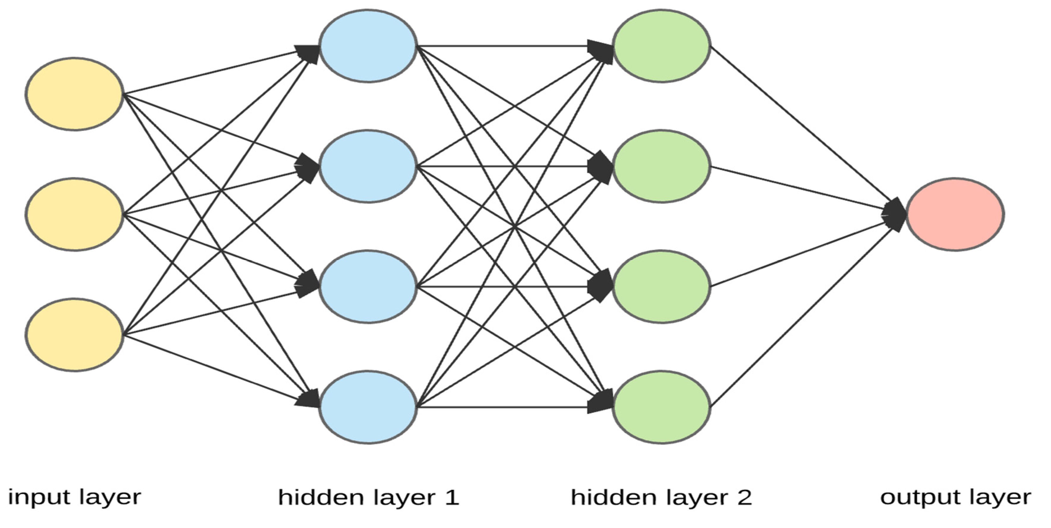
Figure 2.
weight and bias adjustment with activation function. Source: Author’s own.
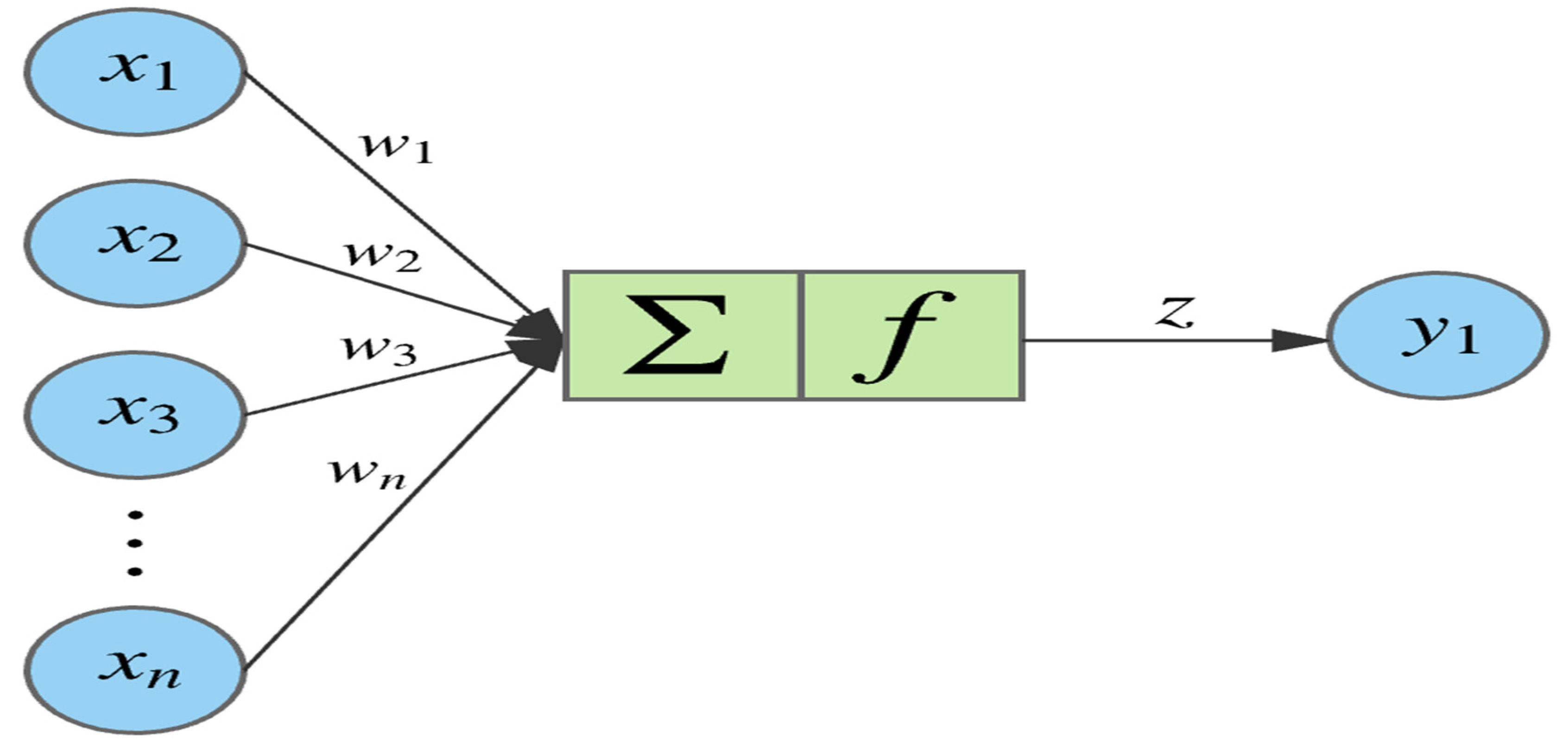
Figure 3.
Skewed data for limit balance and age. Source: Author’s own.
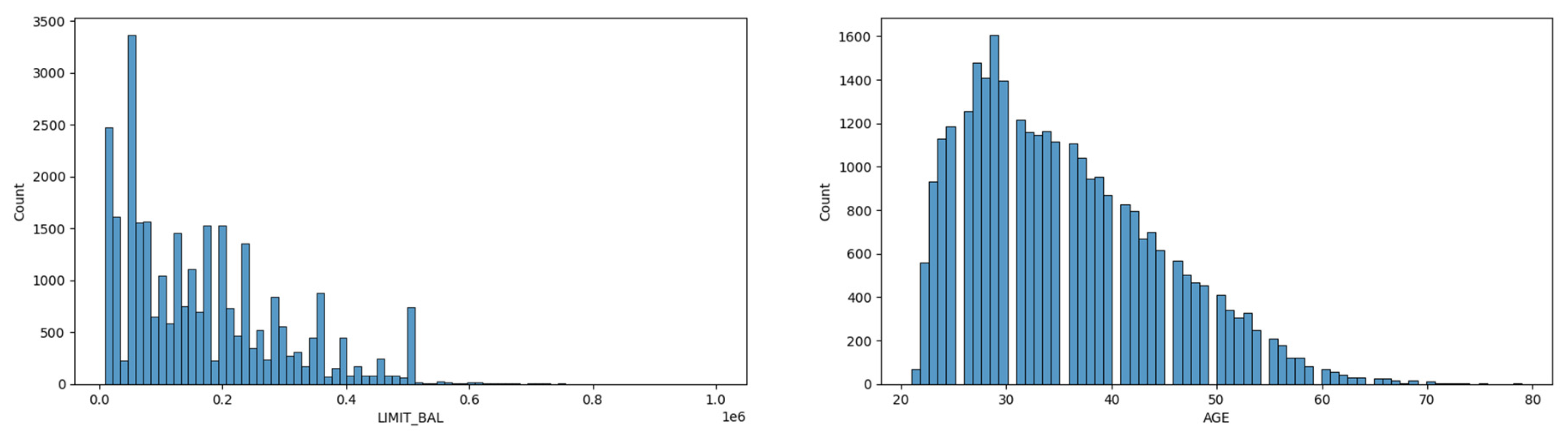
Figure 4.
Heatmap for the various features of the dataset. Source: Author’s own.
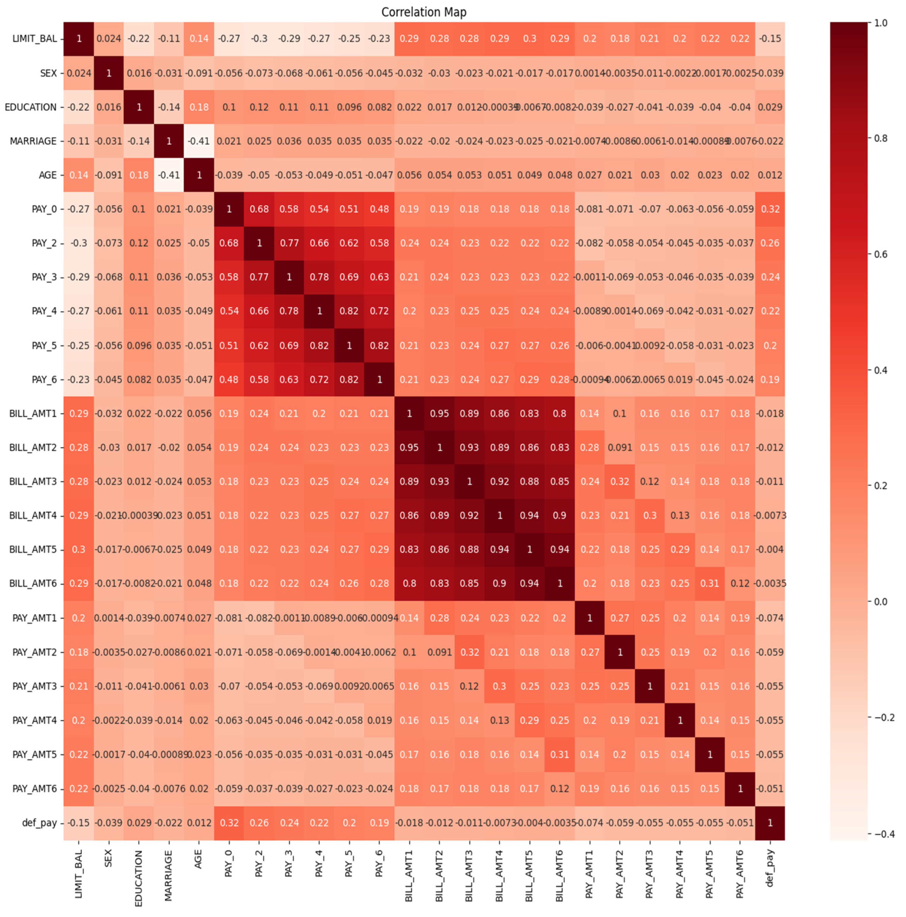
Figure 5.
relationship between bill amount and payment made. Source: Author’s own.
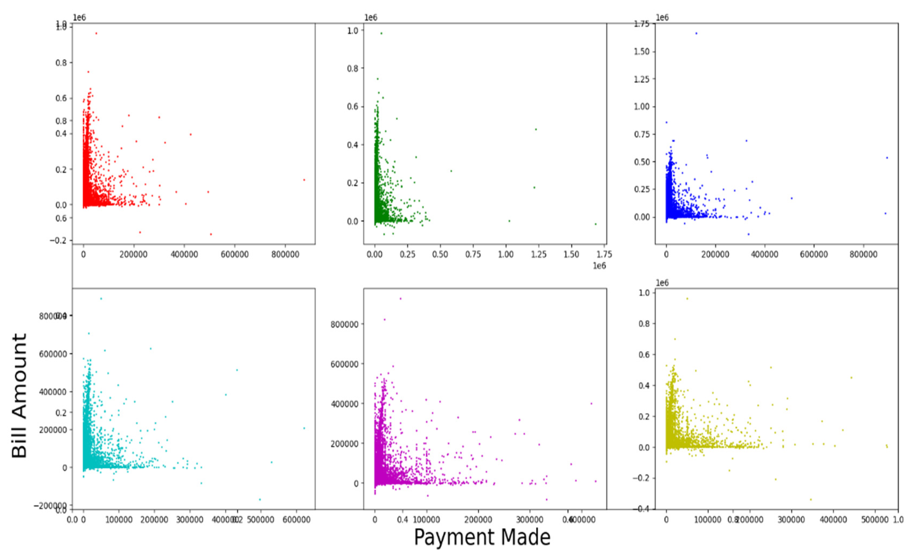
Figure 6.
ROC for the various models. Source: Author’s own.
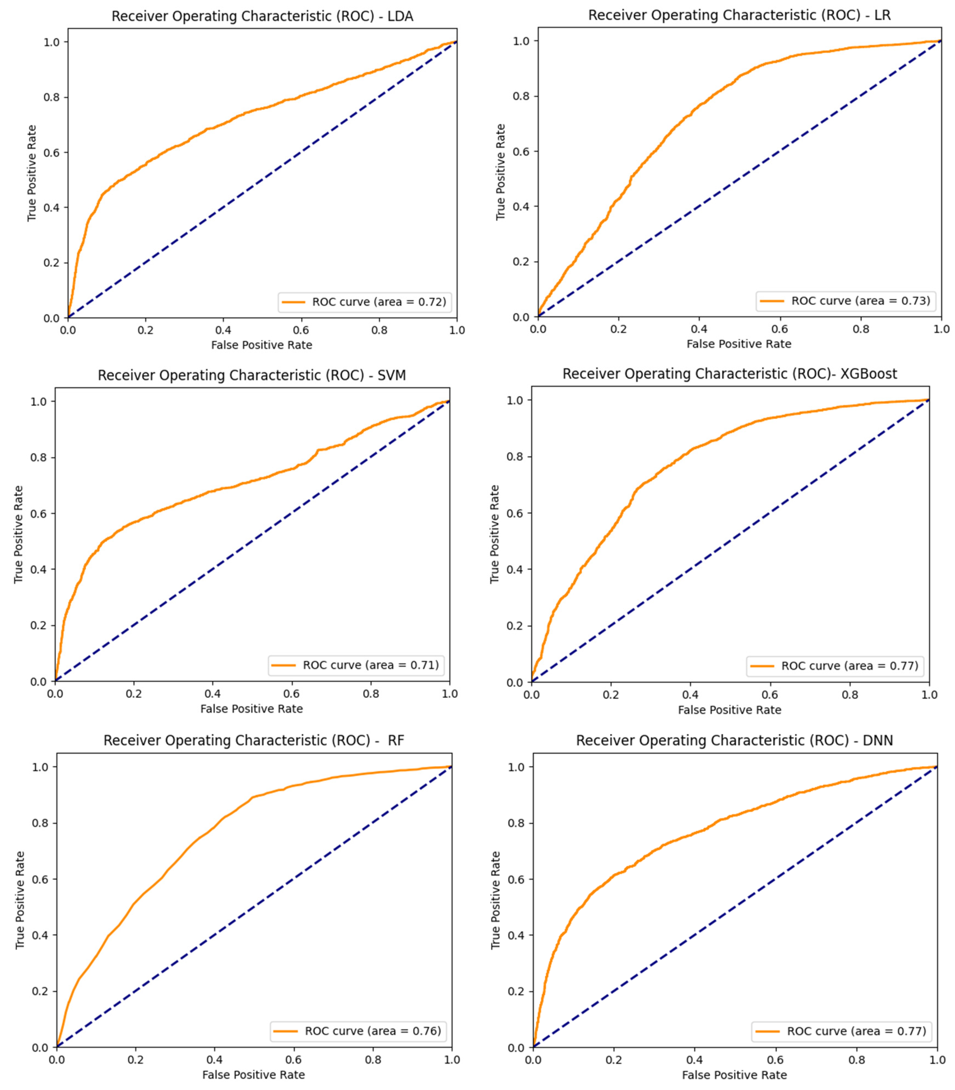
Figure 7.
Features importance for the DNN model. Source: Author’s own.
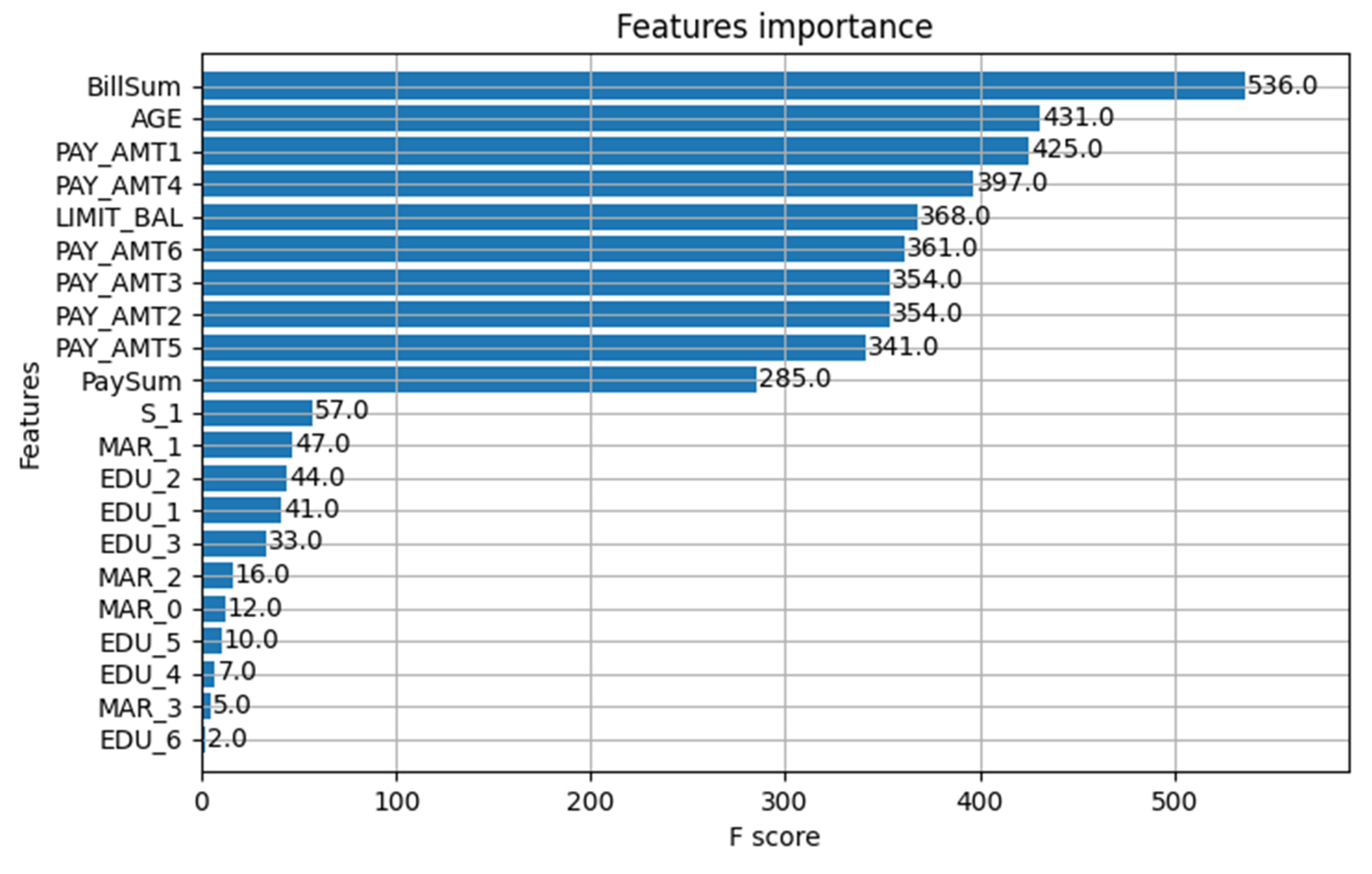

Table 1.
Attributes of the dataset with feature code and description.
| Feature ID | Feature Code | Description |
|---|---|---|
| X1 | Limit_bal | The amount of credit that the card holder is entitled to avail. It includes individual and family credit. |
| X2 | Sex | (Gender) 1=male, 2=female |
| X3 | Education | 1= graduate, 2 = university, 3 = high school, 4=others. |
| X4 | Marital status | 1=Married, 2=Single, 3=Others |
| X5 | Age | 21 years to 79 years |
| X6 to X11 | History of past payment month wise | Repayment status codes-1 = paid duly 1 = payment delay for one month 2 = payment delay for two months … 9 = payment delay for 9 months and above |
| X12 to X17 | Amount of bill statement | X12 = amount of bill statement for September 2005 X13 = amount of bill statement for August 2005 … X17 = amount of bill statement for April 2005 |
| X18 to X23 | Amount of previous payment | X18 = amount paid in September 2005 X19 = amount paid in August 2005 … X23 = amount paid in April 2005 |
Source: (Yeh, 2016).
Table 2.
Confusion Matrix.
| Actual | Prediction | |
| 0 (Negative) | 1 (Positive) | |
| 0 (Negative) | True Negative (TN) | False Postive (FP) |
| 1 (Positive) | False Negative (FN) | True Positive (TP) |
Source (Bekkar et al., 2013).
Table 3.
Metric used to assess the model’s performance.
| Metric | Formula |
|---|---|
| Accuracy | |
| Error rate = 1 - Accuracy | |
| Sensitivity (or Recall, Accuracy of positive examples) | |
| Specificity (Accuracy of Negative examples) | |
| Prescision | |
| F1-Score | 2* |
| G-mean |
Source (Bekkar et al., 2013).
Table 4.
Confusion Matrix for the various models.
| LDA | LR | SVM | ||||||
|---|---|---|---|---|---|---|---|---|
| Actual | Prediction | Actual | Prediction | Actual | Prediction | |||
| 0 | 1 | 0 | 1 | 0 | 1 | |||
| 0 | 4529 | 158 | 0 | 4549 | 138 | 0 | 4560 | 127 |
| 1 | 988 | 325 | 1 | 1002 | 311 | 1 | 1010 | 303 |
| XGBoost | RF | DNN | ||||||
| Actual | Prediction | Actual | Prediction | Actual | Prediction | |||
| 0 | 1 | 0 | 1 | 0 | 1 | |||
| 0 | 4406 | 281 | 0 | 4417 | 270 | 0 | 4400 | 287 |
| 1 | 819 | 494 | 1 | 832 | 481 | 1 | 805 | 508 |
Source: Author’s own.
Table 5.
Performance metrics for the various models.
| Mertric | LDA | LR | SVM | XGBoost | RF | DNN |
|---|---|---|---|---|---|---|
| Accuracy | 0.8090 | 0.8100 | 0.8105 | 0.8167 | 0.8163 | 0.8180 |
| Sensitivity or Recall | 0.2475 | 0.2369 | 0.2308 | 0.3762 | 0.3663 | 0.3869 |
| Specifivity | 0.9663 | 0.9706 | 0.9729 | 0.9400 | 0.9424 | 0.9388 |
| Precision | 0.6729 | 0.6927 | 0.7047 | 0.6374 | 0.6405 | 0.6390 |
| F1 Score | 0.3619 | 0.3530 | 0.3477 | 0.4732 | 0.4661 | 0.4820 |
| G—mean | 0.4891 | 0.4794 | 0.4738 | 0.5947 | 0.5876 | 0.6027 |
| AUC | 0.72 | 0.73 | 0.71 | 0.77 | 0.76 | 0.77 |
Source: Author’s own.
Disclaimer/Publisher’s Note: The statements, opinions and data contained in all publications are solely those of the individual author(s) and contributor(s) and not of MDPI and/or the editor(s). MDPI and/or the editor(s) disclaim responsibility for any injury to people or property resulting from any ideas, methods, instructions or products referred to in the content. |
© 2024 by the authors. Licensee MDPI, Basel, Switzerland. This article is an open access article distributed under the terms and conditions of the Creative Commons Attribution (CC BY) license (http://creativecommons.org/licenses/by/4.0/).
Copyright: This open access article is published under a Creative Commons CC BY 4.0 license, which permit the free download, distribution, and reuse, provided that the author and preprint are cited in any reuse.


