
Submitted:
30 August 2024
Posted:
09 September 2024
You are already at the latest version
Abstract
In this work, we study a boundary control problem for the evolutionary Stokes equations, under mixed boundary conditions, in two and three dimensions. The Stokes equation is a valuable tool in cardiovascular biomechanics, especially for modeling blood flow in low-velocity and high-viscosity conditions. Its application in the microvasculature, the design of medical devices, and the study of cardiovascular diseases helps improve the understanding and treatment of various pathological conditions. We provide a comprehensive theoretical framework to address the analysis and the derivation of a system of first-order optimality conditions that characterizes the solution of the control problem. Finally, solution-finding algorithm is proposed and illustrated with some simulations.
Keywords:
optimal control
; partial differential equations
; fluid dynamics
; stokes equation
; total stress
; boundary control
; finite element method
1. Introduction
Optimal control problems of systems governed by partial differential equations (PDEs) have garnered significant attention in recent decades. The Stokes equations, a simplified version of the Navier-Stokes equations, are pivotal in describing the flow behavior of incompressible fluids under low Reynolds number conditions where viscous forces dominate inertial forces. These problems may be applied in different science and engineering fields such as atmospheric and ocean sciences, aeronautics, and industrial design. In [15,25], several relevant topics related to both theoretical and numerical aspects may be found, as a result of, at least, a decade of research by different authors. More recently, the application of flow control to computational blood flow modeling has also been investigated. Examples can be seen in [4,14], for the stationary case, or [7] for time-dependent equations.
From the applications point of view, the Stokes and Navier-Stokes equations have been complemented with Dirichlet boundary conditions, mixed with imposed stress conditions, also known as traction boundary conditions. Nevertheless, as it was indicated in [8], for the purpose of considering the coupling of the fluid with a model representing the blood vessel wall, imposing the so-called total stress vector, instead of the usual stress vector, should be preferred.
Optimal control problems, in general, aim to determine control inputs that optimize a given performance criterion while ensuring that the system dynamics adhere to certain constraints. When these systems are governed by partial differential equations (PDEs) like the Stokes equations, the complexity of the control problems increases significantly. In particular, boundary optimal control problems involve finding controls applied on the boundary of the domain to achieve desired outcomes within the fluid flow.
Mixed boundary conditions, combining Dirichlet and stress (Neumann) conditions, add another layer of complexity to these control problems. While Dirichlet conditions, which specify the value of the function on the boundary, are well-understood and lend themselves to classical regularity results, the introduction of stress conditions complicates the analysis. Mixed boundary conditions often lead to a loss of regularity that poses significant challenges in both the theoretical and numerical study of these problems. In this sense, following the approach from [1,2], they employ mixed boundary conditions, including the homogeneous Dirichlet condition for the pressure on a portion of the boundary of the flow domain; but at the same time, they formulate the optimal control problem without using the curl operator and boundary conditions associated with this operator. However, in [1] they take into account the dependence of both the viscosity and the thermal conductivity coefficient on the temperature. This expands the range of possible applications of the results. But, in our case, we consider a phisical model based on the Stokes equations where the viscosity is a real positive constant and we do not consider viscosity to be dependent on temperature. This is justified by the specific medical applications we are focusing on, where the viscosity of blood can be considered constant. The temperature variations in these scenarios are minimal and do not significantly affect the viscosity. Therefore, assuming constant viscosity simplifies the model without compromising the accuracy of the results within the application we want to study.
In this work, we analyse the boundary optimal control problem associated with the time dependent Stokes equation under mixed Dirichlet and total stress boundary conditions. The boundary of the domain is assumed to be composed of three distinct components. A fixed total-stress condition is assumed on one part, a homogeneous Dirichlet condition on another and, finally, a Dirichlet-type control is assumed to act on the remaining third component. This configuration is inspired by the applications addressed in [7,14]. There, a Dirichlet control was applied at the inlet boundary, stress conditions were considered on the outlet boundaries, whereas homogeneous Dirichlet conditions were associated with the physical no-slip assumption. In those works, the stress boundary condition is to be understood as a prescribed force per unit area, computed as the normal component of the Cauchy stress tensor.
The application of the Stokes equations in cardiovascular problems is particularly noteworthy. In modeling blood flow in microcirculation and small arteries, where the flow is typically slow and viscosity effects are pronounced, the Stokes equations provide a more appropriate model than the full Navier-Stokes equations. In such contexts, optimal control techniques are used to simulate and control blood flow, aiming to improve the understanding and treatment of cardiovascular diseases.
Recent studies have applied these principles to computational blood flow modeling. For instance, Dirichlet boundary conditions are used to model the no-slip condition on vessel walls, while stress conditions are applied at the interfaces where blood interacts with medical devices or at the outlet boundaries of the vascular network, see [13]. These mixed boundary conditions mimic physiological conditions more accurately but also introduce additional analytical challenges due to the loss of regularity.
The coupling of fluid flow with models representing the artery walls, often referred to as fluid-structure interaction (FSI) problems, further complicates the scenario. Here, the use of total stress boundary conditions, which account for both pressure and viscous stress, becomes crucial. These conditions are essential for accurately modeling the interaction between blood flow and arterial walls but require advanced mathematical techniques to handle the resulting optimal control problems.
Boundary control problems, under the stationary assumption, have long been studied by different authors. Concerning mixed boundary conditions of Dirichlet-Neumann (stress vector) type, in [11] a Neumann-type control problem is studied. There, the goal was the drag minimization, under state constraints, on a two-dimensional exterior problem. Following some of those ideas, in [13], the existence of an optimal boundary control was established under different types of cost functionals, motivated by some of the aforementioned applications. In [23], the authors used a Lagrange multipliers approach to address the control of the Dirichlet boundary, still in the stationary case.
Concerning time-dependent problems, Dirichlet controls have been considered in [18,21,22] for bounded domains in 2D. In [10], the authors considered a Dirichlet control acting on an interior boundary of an unbounded 3D domain. The case of mixed boundary conditions, particularly of the case of Dirichlet-Total Stress remains, up to our knowledge, to be analysed.
Our work aims to provide a deeper understanding of mixed boundary optimal control problems for the time-dependent Stokes equations, particularly in the context of cardiovascular applications. We draw inspiration from established methods in the literature, such as those used for Dirichlet controls in bounded domains and mixed Dirichlet-Neumann conditions. However, we extend these approaches to handle the more complex mixed boundary conditions of Dirichlet and Total Stress. This extension is non-trivial and requires careful analysis to ensure the existence and regularity of solutions, addressing the unique challenges posed by the loss of classical regularity, see [24].
In this sense, our domain is an idealized domain representing a partially obstructed vessel capillary. The domain is represented in Figure 1. In this case, the left side is the inlet boundary (where we imposed the control) while the right side corresponds to outlet boundary (where we imposed the total stress condition). The remaining boundaries represent the vessel wall where we imposed homogeneous Dirichlet conditions.
Moreover, this work aims to serve as a foundational study for future research in the control of the Navier-Stokes equations and fluid-structure interaction problems. By establishing a robust theoretical and numerical framework for the Stokes equation, we try to pave the way for addressing these more complex and realistic problems, ultimately contributing to the advancement of optimal control techniques in cardiovascular applications.
The plan of this paper reads as follows. In Section 2 we present an analysis of the direct problem, i.e., the Stokes equation with mixed boundary conditions. This section provides the mathematical setting for the analysis of the optimal control problem, which will be the subject of Section 3. In the later, existence of solution and first order conditions are studied. In Section 4, we provide numerical results and we finish by summarizing some conclusions and perspectives.
2. Unsteady Stokes Equation
In this section, we consider the direct problem, that is, the non-stationary Stokes equation with mixed boundary conditions of Dirichlet and total stress types.
Despite their relevance when modeling viscous incompressible flows, the Stokes equation, endowed with such type of mixed boundary conditions, have been seldom analysed from a theoretical standpoint. An exception are the results found in [3,20], for the homogeneous case. As explained by the authors there, one of the advantages of this configuration is the possibility of deriving an energy inequality, contrary to the configuration based on the ubiquitously used stress (Neumann) boundary conditions, for which no control over the energy flux can be achieved.
We can describe our problem as follows. Given functions and the initial condition , we want to solve system
where the unknowns are the fluid velocity u and the pressure p, is the exterior unit normal to and is the boundary of an open bounded domain with .
Now, we provide a brief nomenclature below that defines the physical parameters and symbols used throughout this paper. This nomenclature is try to help readers fully understand the equations and the model presented in the study and to apply the study to the medical cases.
- Kinematic viscosity of the fluid.
- represents the strain rate tensor.
- external force term applied to the fluid.
- g: control velocity condition at the inlet
- : unit normal vector to the boundary.
- h: boundary condition related to stress on .
- initial velocity.
Under the above assumptions, we can say that system (1) models an incompressible Newtonian fluid at a constant temperature.
The non-homogeneous Dirichlet condition for the boundary corresponds to what will later be considered as the control action. Also, there is another boundary component, , where we apply a prescribed total stress condition. Finally, in the remaining part of the boundary we impose a homogeneous Dirichlet condition.
Therefore, whenever required, we denote by and as a reference to Dirichlet (essential) and Neumann (natural) boundary conditions, respectively.
2.1. Functional Spaces and Preliminary Results
In this section we introduce some functional spaces along with several properties and preliminary results that will be required later on, for our subsequent analysis.
In the sequel, let be a connected open set of , with a locally Lipschitz boundary composed by three smooth open subsets, mutually disjoint, denoted by , , such that:
For convenience, we introduce the classical space V and H for Stokes equations, but we adapt the definitions to the boundary conditions:
where is the trace operator to a subset
Also, we consider:
and
where is the dual space of and the dual of the
Lemma 1.
The space is dense in and the space V is also dense in
Proof:
Thanks to the Poincaré inequality (it remains true when we have that the functional space and V is null on a part of boundary), we have that and are continuous embeddings. Then, the conclusion follows from the classical results found in [26], Chapter 1.2.
□
Note that, from the definition of the functional spaces, and thanks to Riesz’s Theorem, we also have the following chain of continuous injections:
In addition, by using Lemma 1.1 (Chapter III) of [26], we can ensure that and
In the sequel, we consider to be the usual norm, and we denote by the inner product in . Also, we consider and to be the norma in and respectively, defined by
Besides, we denote by the usual inner product. When convenient, we represent and by and , respectively, for example:
2.2. Existence and Uniqueness Result
This section is devoted to the existence of a solution for the Stokes equation (1). To this purpose, we start by introducing the weak formulation as well as the definition of a weak solution of these equations.
Definition 1.
Notice that, the pressure is not appearing in the weak formulation. Nevertheless, as in the cases with a single Dirichlet condition is considered, we can recover the pressure using De Rham’s - type results ([26]). We could also consider a mixed weak formulation that includes pressure in the problem’s formulation. In this case, the solution space would change and would no longer include the condition of zero divergence. Accordingly, this equation would also be incorporated into the weak formulation as an additional equation, allowing us to solve for the pressure as well.
Because we are going to use the Dirichlet boundary condition as a control variable, let us assume some additional requirements for g. We recall the following result
Lemma 2.
There exists a bounded extension operator , where
with the tangential gradient.
Note that, the tangential gradient of f at a point is defined as the tangential component of the gradient of the trace of f, i.e., the projection of the gradient of the trace of f onto the tangent plane to at x, that is,
wher is the trace of f on .
The proof of this lemma follows the proof of the Corollary 3.5 of [11].
In order to extend the E operator to the time domain, see that
Lemma 3.
Let a real number , then, there exists a bounded extension operator , with
Proof:
We use the definition of the operator to prove that it is bounded. Let ,
where doesn’t depend on t by the definition of bounded operator. So, we have that:
Therefore, is well defined and is a bounded operator.
□
The existence of such extension operators allows us to define the following set:
which characterizes the Dirichlet boundary conditions that we are going to consider.
At this point, we can state the following existence result
Theorem 1.
Let , be an open boundary set with a locally Lipschitz boundary, , , and with Then, there exists a unique weak solution of the Stokes system (2), satisfying:
Proof:
We start by remarking that there exists a function with and with .
Then, and for all we have that
Next, consider the following homogeneous problem:
We use the compacity method and Galerkin approximation to prove the existence of the solution, as in Theorem 1.1 of Chapter III of [26].
So, we can ensure that
□
Note that, the solution then u is equal a.e. to a continuous function , see [26]. This fully clarifies the initial condition in time.
Consequently, these results indicate that mathematically, there is a unique weak solution, which physically implies that the proposed problem is well-posed and can be solved. In other words, for any desired initial data, the Stokes equation can be used to approximate blood flow.
3. Optimal Control Problem
This section is devoted to the study of the optimal control problem associated to the Stokes Equation (2).
3.1. Existence of an Optimal Pair
Consider the quadratic functional defined by:
where are positive given constants and , are given functions and is the tangential gradient in .
Consider also the admissible control set:
and the feasible set
The problem that we intend to solve in this section is the following:
Find such that
The existence of an optimal control can then be ensured as follows.
Theorem 2.
Let , , be an open boundary set with a locally Lipschitz boundary, , and . Then, there exists a pair solution of (6).
Proof:
Firstly, notice that if we consider for instance to be null, thanks to Theorem 1, we can immediately see that the feasible set is non-empty. Since for all , which is non-empty, there exists a minimizing sequence such that
Also,
Therefore, is uniformly bounded in .
Besides, there exists with the bounded extension operator defined in Lemma 3. Since and , then in uniformly bounded in .
Taking into account that are the corresponding solutions of the weak Stokes equation, by using the estimates, we conclude that is an uniformly bounded sequence in
Hence, we can extract at least a subsequence, still renamed as , which weakly converges to a certain pair .
Moreover, there exists a pair such that, at least for a subsequence,
Inserting into (2) we obtain:
We can, therefore, conclude that belongs to . Finally, as J is coercive and lower semicontinuous with respect to the weak convergence, we conclude that
and is a minimizer.
□
3.2. Differentiability and Characterisation Results
Differentiability is an important issue in the study of optimal control problems, as it allows the derivation of the first order optimality conditions which provide further characterisation of the optimal pair.
With this aim, we will follow an approach that is inspired in [21], for the case of a single boundary condition.
We start by introducing two auxiliary systems which are related, respectively, to the linearized and the adjoint state equations which will later be used for the optimality conditions:
and
We can give the following regularity result:
Proposition 1.
The weak formulations of (7) and (8), although associated to linear problems, include transport type terms that can be recast into the frame of Theorem 1.
Let us now write problem (6) as:
where .
In this case, with
with and
Proposition 2.
The mapping is twice continuously Fréchet differentiable with local Lipschitz continuous second derivative.
Note that, the differentiability of the linear operators is immediate. So, we can then conclude that the application and are continuous and twice continuously Fréchet differentiable, and the second derivative is Lipschitz continuous.
We are now in conditions to provide a necessary condition that characterizes the optimal solution, known to exist thanks to Theorem (2).
In the sequel, we denote by the list of assumptions:
Theorem 3.
Let be satisfied and a minimum provided by Theorem 2, then there exists an adjoint state and an adjoint pressure such that verify:
and
and
Proof:
Note that, as we have a unique solution each control g, we can identify the reduced cost functional, i.e, we can write that
Remark that the above reasoning is possible because we have a uniqueness result for the Stokes equations. In case of not having a uniqueness of solution, as in the 3D case of Navier-Stokes equations, this classical reasoning could not be used and we would have to resort to more advanced techniques to the proof. Specifically, we could try to follow the reasoning already used in other works, such as [5,6], in which a uniqueness of solution was not assumed.
It is easy to check that J is Gâteaux differentiable, and
with v solution of:
Therefore, integrating by parts we obtain:
for all with the adjoint state associated (9b) to the weak solution to Stokes equations (9a) with
Note that our problem satisfies the conditions of Theorem 9.6 of [24]:
- J and e are Fréchet differentiable, thanks to Proposition 2.
- For each , the state equation defines a unique control-to-state map , that is for any , thanks to the uniqueness result proved in Theorem 1. Moreover, the control-to-state map is Gateaux differentiable, thanks to Proposition 2.
-
The partial derivative is a continuous isomorphism. In fact, thanks to Proposition 2, where withwith andAs a consequence of Proposition 1, the mapping is a homeomorphism. Hence by Proposition 2 and the Implicit Function Theorem the first derivative at can be expressed as
Hence, in view of that result, we can ensure that, if is a minimum control provided by Theorem 2 associated to the state u, then there exists an adjoint pair of state and pressure variables satisfying the optimality system.
□
If we want to consider strong solution, then the optimality system is:
and
and
These results allow us to conclude that the boundary control problem has a unique solution and we can compute it by using the optimallity system. From an application perspective, this means that for any desired data, it is possible to control the blood flow by adjusting only the fluid inlet profile, thereby directing the flow to achieve a desired and optimal movement for proper functioning.
4. Algorithm and Numerical Simulations
In the previous sections, we have conducted a theoretical study that has allowed us to characterize the optimal control. In particular, we have obtained an adjoint variable that enables us to calculate the gradient of the reduced cost. The gradient calculation is the main ingredient of the so-called descent methods. Thus, classic descent algorithms such as the gradient method will be proposed.
ALG: Optimal Step Gradient Method
- (a)
- Choose and
- (b)
Note that, we are considering that is due to our is a vertical line.
Let us now provide further details on the numerical approximation used to solve (11) and (12). We start by introducing the variational form of the equations and then, we discretize our systems in time, by using the backward implicit Euler finite difference. Finally, we use the finite element method to discretize in space. Consequently, the discrete problems solved at each iteration are:
with the corresponding test functions and (being u, p the iterate of the algorithm) for . Similarly, we have:
On the other hand, in the numerical experiment, we use an explicit approximation formula to compute the optimal step . For a given search direction d, we introduce the linearization of the mapping And the optimal step is given by the expression with So the unique root of the is given by:
where v is the solution to the homogeneous Stokes system with
- Test: 2D stenotic vessel capillary with noise data
Our test addressed an idealized domain representing a partially obstructed vessel capillary, and we aimed to approximate the solution to a noisy solution in order to simulate the noise obtained from medical tests
The domain is represented in Figure 2. In this case, the left side is the inlet boundary (where we imposed the control) while the right side corresponds to outlet boundary (where we imposed the total stress condition). The remaining boundaries represent the vessel wall where we imposed homogeneous Dirichlet conditions.
In order to solve numerically the systems appearing in ALG, we had to fix a mesh, the finite element approximation spaces, and a time step. For the space discretization, we used a mixed finite element formulation with continuous piece-wise P2 and P1 functions for the velocity field and the pressure, respectively. For details, see [12]. The simulations for the current test, as well as for the following ones, have been performed with the FreeFem++ package (see [19]).
We take , , , considering stationary total stress . We want to drive the solution close to desired states, and , where is a noisy perturbation of the solution of (16), and :
We considered, as intial guess for the control,
We will now present relative error for different experiments in which we have varied the Reynolds number and the noise rate of the data. It is important to note that in this case, we have chosen small Reynolds numbers (on the order of and ) because these correspond to the Reynolds number of blood in capillaries, which is where these equations can be applied. In the following table, see Figure 3, the relative errors between the calculated solution and the desired noiseless solution will be shown:
As can be observed in Figure 3, the algorithm performs quite well and successfully approximates the solution even when the noise levels in the data exceed It is also notable that, as expected, when we decrease the value of , the relative errors increase, although they remain small. All of this suggests that the algorithm works efficiently and quickly converges to a solution that is very close to the desired one.
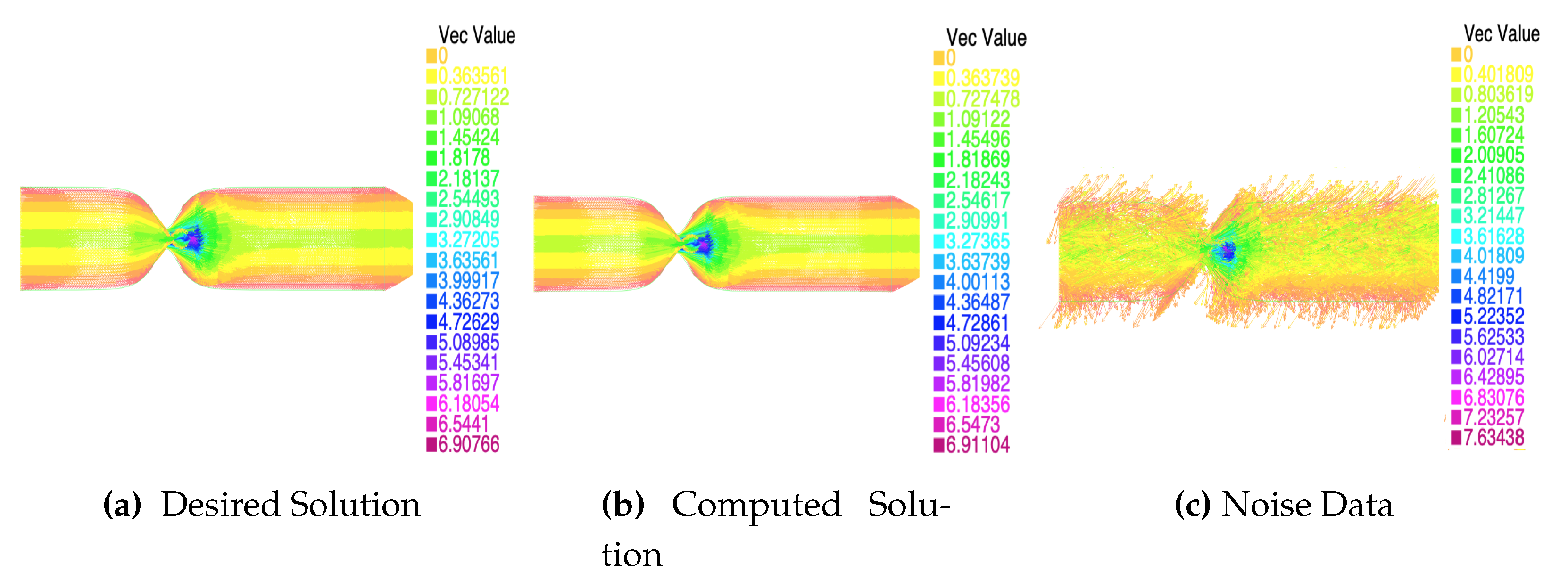
Next, we will present the solution obtained for a specific case at three different times throughout the interval , see Figure 4, Figure 5 and Figure 6.
As can be seen in the images, see Figure 4, Figure 5 and Figure 6, the solution obtained with the algorithm is very close to the desired noiseless solution, even when we have high levels of noise in the data, as is the case here. Specifically, it should be noted that the noise is introduced into the Stokes equation due to the adjoint state, but as we can see, the algorithm is able to suppress that noise and find the noiseless solution. This aspect is very important from the perspective of application and the use of medical data, as data obtained from medical tests often have a high noise rate. Therefore, it is a very positive aspect that the algorithm is capable of overcoming this problem.
5. Conclusions
In this work, we have provided necessary conditions for a boundary control problem associated with the time-dependent Stokes equations, under boundary conditions of mixed type. In a certain sense, it can be seen as an extension of the work performed in [13], to the the time-dependent case under mixed boundary conditions. We could see that an initial guess, associated with a noise can be improved until decreasing the relative fitting error to less than This is the case, even when high noise rate are considered, as well as nonphysical data.
One of the major contributions of this work is to lay the groundwork for extending it to the time dependent case. It is important to note that this extension is by no means trivial, and we are currently working on it. One of the key aspects to consider, if we want to extend the work to the Navier-Stokes equations in the two-dimensional case us that we don’t have a linarity equation so we have to use another technique to get the results. Moreover, in the three-dimensional case, we do not have uniqueness of solution nor good regularity even with Dirichlet-type conditions. Therefore, in the three-dimensional case, it will be necessary to work under the assumption that a unique solution exists and assuming sufficient regularity to dprove similar results to those presented in this work. Additionally, since gradient-type algorithms are known to become computationally expensive, parameterized approaches are now being considered for 3D simulations. Future extensions may consider with Navier-Stokes equations, as well as multiple boundary controls.
Funding
This research received no external funding.
Conflicts of Interest
The authors declare no conflicts of interest.
References
- Baranovskii, E.S. Feedback optimal control problem for a network model of viscous fluid flows. Math. Notes 2022, 112, 26–39. [Google Scholar] [CrossRef]
- Baranovskii, E.S.; Domnich, A.A.; Artemov, M.A. Optimal boundary control of non-isothermal viscous fluid flow. Fluids 2019, 4, 133. [Google Scholar] [CrossRef]
- Bernard, J. Time-dependent Stokes and Navier-Stokes problems with boundary conditions involving pressure, existence and regularity. Nonlinear-Anal. World-Appl. World App 2003, 4, 805–839. [Google Scholar] [CrossRef]
- Delia, M.; Perego, M.; Veneziani, A. ; A Variational Data Assimilation Procedure for the Incompressible Navier-Stokes Equations in Hemodynamics. J. Sci. Comput. 2011, 52, 340–359. [Google Scholar] [CrossRef]
- E. Fernández-Cara and I. Marín-Gayte, Theoretical and numerical bi-objective optimal control: Nash equilibria. ESAIM Control Optim. Calc. Var. 2021, 27, 50.
- E. Fernández-Cara and I. Marín-Gayte, Theoretical and numerical results for some bi-objective optimal control problems. Commun. Pure Appl. Anal. 2020, 19, 2110–2126. [Google Scholar]
- S. W. Funke, M. Nordaas, O. Evju, M.S. Alnaes, and K.A. Mardal, Variational data assimilation for transient blood flow simulations: Cerebral aneurysms as an illustrative example. Int J Numer Method Biomed Eng 2019, 35, e3152. [Google Scholar] [CrossRef]
- L. Formaggia, A. Moura, and F. Nobile, On the stability of the coupling of 3D and 1D fluid-structure interaction models for blood flow simulations. Esaim Math. Model. Numer. Anal.- ModÉlisation MathÉmatique Anal. NumÉrique 2007, 41, 743–769. [Google Scholar] [CrossRef]
- A. V. Fursikov (ed.), Optimal Control of Distributed Systems: Theory and Applications; American Mathematical Society, Boston, MA, USA, 2000.
- Fursikov, A.V.; Gunzburger, M.D.; Hou, L. Optimal boundary control for the evolutionary Navier–Stokes system: The three-dimensional case. Siam Control. Optim 2005, 43, 2191–2232. [Google Scholar] [CrossRef]
- A. V. Fursikov and R. Rannacher (eds.), Optimal Neumann Control for the Two-Dimensional Steady-State Navier-Stokes Equations, Editors, New Directions in Mathematical Fluid Mechanics: The Alexander V. Kazhikhov Memorial Volume, Basel: Birkhauser, 2010.
- R. Glowinski (ed.), Finite Element Methods for Incompressible Viscous Flow, Handbook of Numerical Analysis, 9, Amsterdam, 2003.
- T. Guerra, A. Sequeira, and J. Tiago, Existence of optimal boundary control for the Navier-Stokes equations with mixed boundary conditions. Port Math 2015, 72, 267–283. [Google Scholar] [CrossRef] [PubMed]
- T. Guerra, C. Catarino, T. Mestre, S. Santos, J. Tiago, and A. Sequeira, A data assimilation approach for non-Newtonian blood flow simulations in 3D geometries. Appl. Math. Comput. 2018, 321, 176–194. [Google Scholar] [CrossRef]
- M. D. Gunzburger (ed.), Flow Control, Springer-Verlag, New York, 1995.
- M. D. Gunzburger, L. Hou, and T.P. Svobodny, Boundary velocity control of incompressible flow with an application to viscous drag reduction. SIAM J Control Optim 1992, 30, 167–181. [Google Scholar] [CrossRef]
- M. D. Gunzburger, L. Hou, and T.P. Svobodny, Analysis and finite element approximation of optimal control problems for the stationary Navier-Stokes equations with Dirichlet controls. ESAIM: Math Model Numer Anal 1991, 25, 711–748. [Google Scholar] [CrossRef]
- M. D. Gunzburger and S. Manservisi, The velocity tracking problem for Navier-Stokes flows with boundary control. SIAM J Control Optim 2000, 39, 594–634. [Google Scholar] [CrossRef]
- F. Hecht, http://www.freefem.org.
- J. G. Heywood, R. Rannacher, and S. Turek, Artificial boundaries and flux and pressure conditions for the incompressible Navier–Stokes equations. Int. J. Numer. Meth. Fluids 1996, 22, 325–352. [Google Scholar] [CrossRef]
- M. Hinze and K. Kunisch, Second order methods for boundary control of the instationary Navier-Stokes system. Zamm-Journal Appl. Math. Mech. Appl. Math. Mech. 2004, 84, 171–187. [Google Scholar] [CrossRef]
- H. Kim, A boundary control problem for vorticity minimization in time-dependent 2D Navier-Stokes equations. Korean J Math 2006, 23, 293–312. [Google Scholar]
- A. Manzoni, A. Quarteroni, and S. Salsa, A saddle point approach to an optimal boundary control problem for steady Navier-Stokes equations. Math. Eng. 2019, 1, 252–280. [Google Scholar] [CrossRef]
- A. Manzoni, A. A. Manzoni, A. Quarteroni, and S. Salsa (eds.), Optimal Control of Partial Differential Equations, Applied Mathematical Sciences, Springer, Cham, 2021.
- S. Sritharan (ed.), Optimal Control of Viscous Flow, SIAM, Philadelphia, 1998.
- R. Temam (ed.), Navier-Stokes equations. Theory and numerical analysis, Studies in Mathematics and Applications.
Figure 1.
Schematic representation of the model.

Figure 2.
The domain and the mesh; is composed of (the left side), (the right side) and (the remaining of boundary).
Figure 2.
The domain and the mesh; is composed of (the left side), (the right side) and (the remaining of boundary).
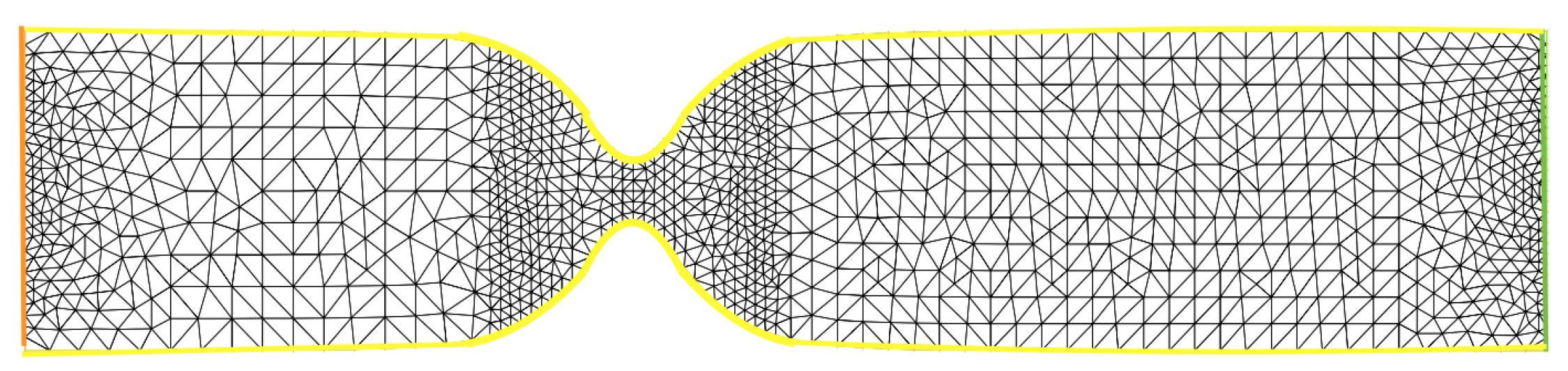
Figure 3.
Relative errors for and .
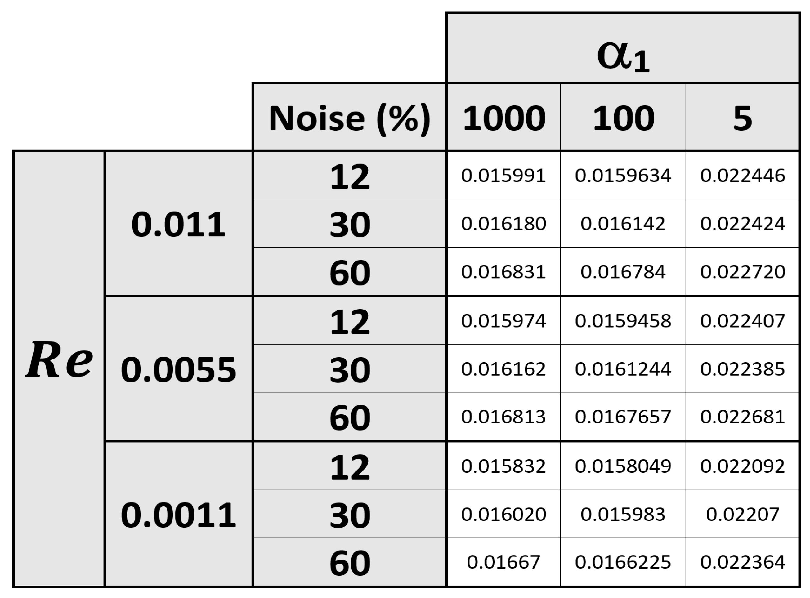
Figure 4.
The velocity fields for and , , , and , with a noise rate of .
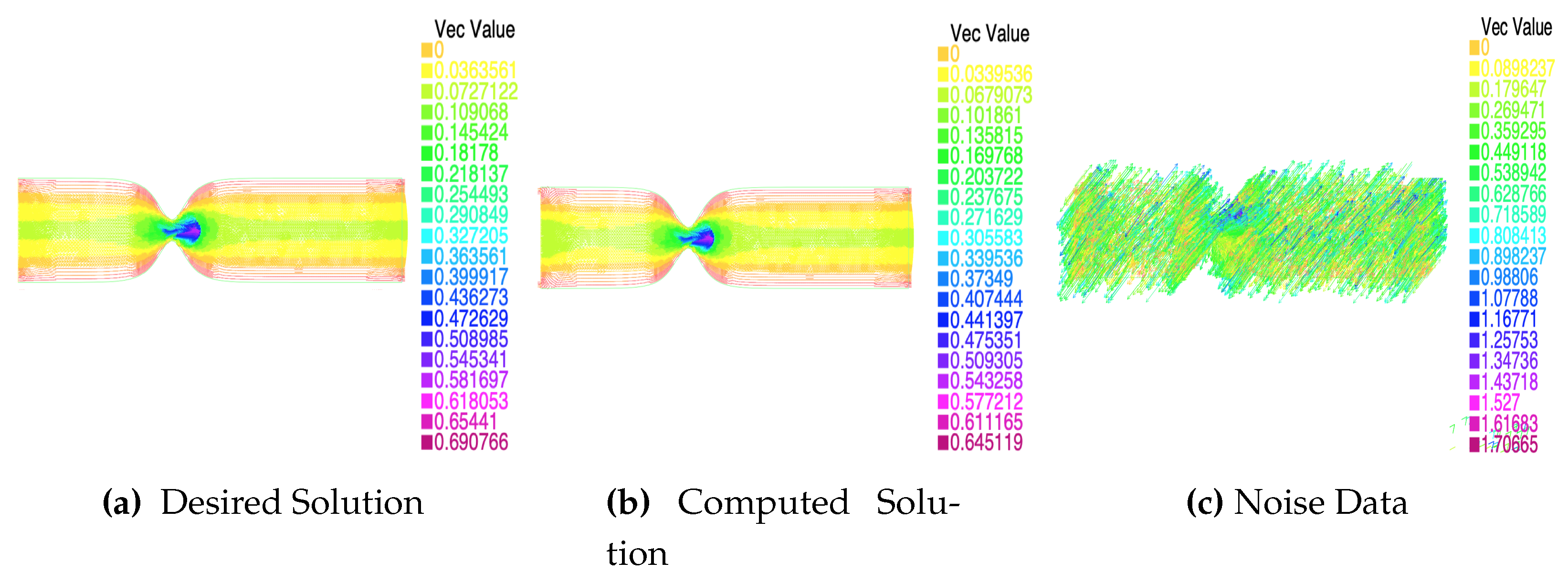
Figure 5.
The velocity fields for and , , , and , with a noise rate of .
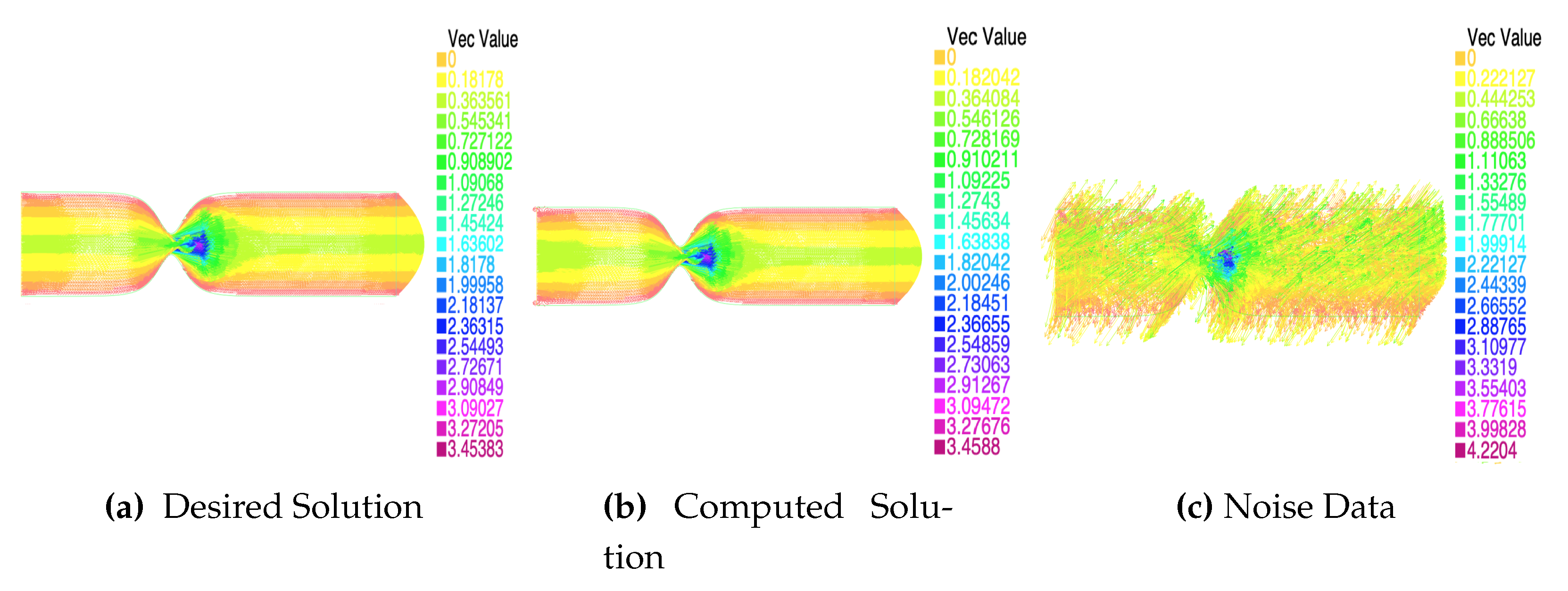
Figure 6.
The velocity fields for the final time and , , , and , with a noise rate of .
Disclaimer/Publisher’s Note: The statements, opinions and data contained in all publications are solely those of the individual author(s) and contributor(s) and not of MDPI and/or the editor(s). MDPI and/or the editor(s) disclaim responsibility for any injury to people or property resulting from any ideas, methods, instructions or products referred to in the content. |
© 2024 by the authors. Licensee MDPI, Basel, Switzerland. This article is an open access article distributed under the terms and conditions of the Creative Commons Attribution (CC BY) license (http://creativecommons.org/licenses/by/4.0/).
Copyright: This open access article is published under a Creative Commons CC BY 4.0 license, which permit the free download, distribution, and reuse, provided that the author and preprint are cited in any reuse.


