Submitted:
29 August 2024
Posted:
02 September 2024
You are already at the latest version
Abstract
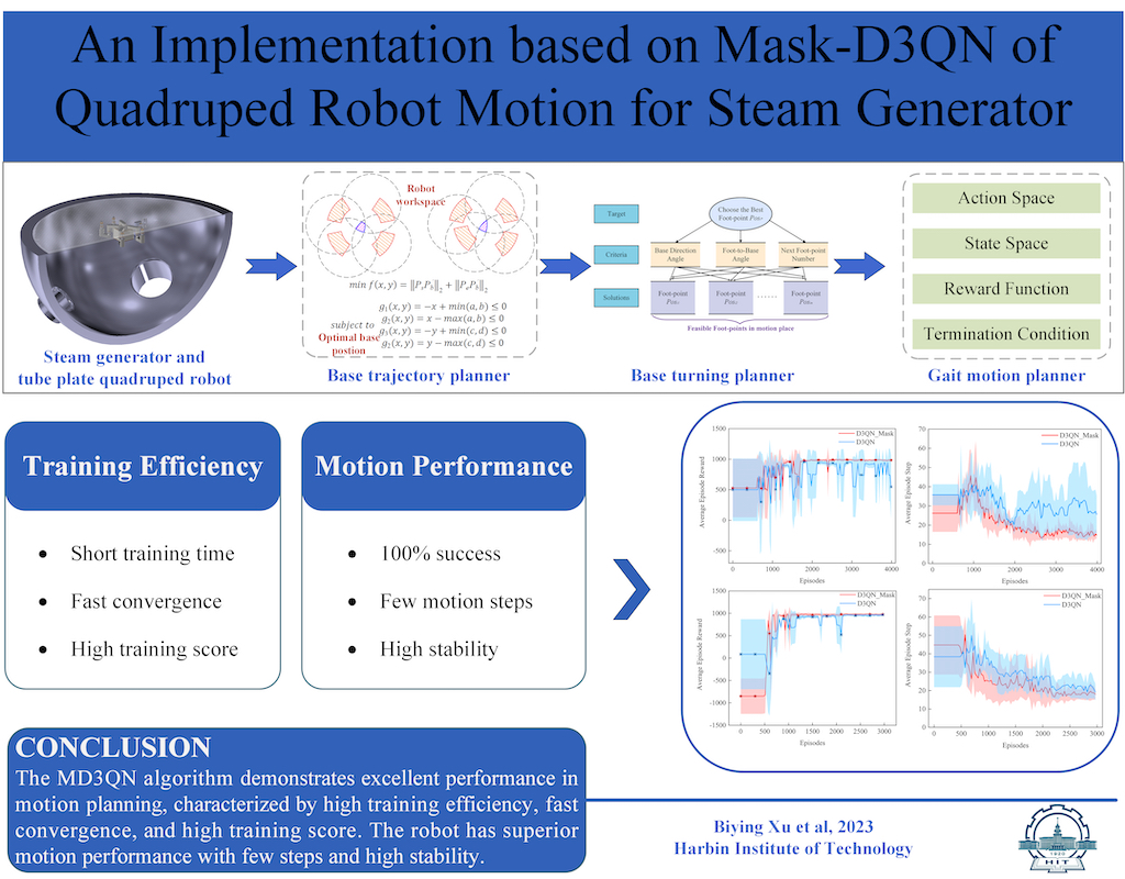
Crawling robots are the focus of intelligent inspection research, and the main feature of this type of robot is the flexibility of in-plane attitude adjustment. The crawling robot HIT_Spibot is a new type of steam generator heat transfer tube inspection robot with a unique mobility capability different from traditional quadrupedal robots. This paper introduces a hierachical motion planning approach for HIT_Spibot, aiming to achieve efficient and agile maneuverability. The proposed method integrates three distinct planners to handle complex motion tasks: a nonlinear optimization-based base motion planner, a TOPSIS-based base orientation planner, and a Mask-D3QN (MD3QN) algorithm-based gait motion planner. Initially, the robot's base and foot workspace are delineated through envelope analysis, followed by trajectory computation using Larangian methods. Subsequently, the TOPSIS algorithm is employed to establish an evaluation framework conducive to foundational turning planning. Finally, the MD3QN algorithm trains foot points to facilitate robot movement along predefined paths. Experimental results demonstrate the method's adaptability across diverse tube structures, showcasing robust performance even in environments with random obstacles. Compared to the D3QN algorithm, MD3QN achieves a 100% success rate, enhances average overall scores by 6.27%, reduces average stride lengths by 39.04%, and attains a stability rate of 58.02%. These results not only validate the effectiveness and practicality of the method but also showcase the significant potential of HIT_Spibot in the field of industrial inspection.
Keywords:
crawling robot
; deep reinforcement learning
; motion planning
; hierarchical planning
1. Introduction
With the rapid development of nuclear energy, research on robots in the nuclear power field has become increasingly prevalent [1]. Within pressurized water reactors of nuclear power plants, the heat transfer tubes within the Steam Generators (SG) serve as critical components for heat exchange, which requires regular inspection and maintenance. How-ever, the specifications of tubes within steam generators vary, as do the distribution of the tube plates. There are many kinds of inspection robots in service, such as ZR-100 [2], PEGASYS [3], HIT-Crawler [4], etc. However, each ro-bot can only be applied to a specific type of steam genera-tor, featuring limited motion capabilities. Consequently, inspection tasks for different steam generators necessitate the corresponding robots, followed by re-installment and recalibration, leading to suboptimal inspection efficiency.
To enhance the adaptability of robots to various types and specifications of tube plates, enabling them to move and inspect tube holes on the plate more flexibly, safely, and efficiently, we have developed a tube plate quadruped inspection robot named HIT_Spibot [5]. Concurrently, the development of a motion planner is required to ensure its rapid and reliable movement along specified paths on the tube plate.
Research on the locomotion of legged robots primarily focuses on ensuring stability, as these robots rely on contact forces such as friction to traverse on the ground. Ensuring stability is particularly crucial to prevent falls or overturning [6]. However, the toes of HIT_Spibot are firmly attached to the tube plate, allowing the robot to remain stable on the plate as long as three feet are fixed. Due to the unique character of the plate and robot structure, the objective of motion planning for tube plate quadruped inspection robots is to achieve flexible and efficient motion planning while ensuring safety. It is noteworthy that, to date, there has been no scholarly investigation into the motion planning of such robots engaged in complex planar movements.
Therefore, this paper proposes a hierarchical planning method for the tube plate quadruped inspection robot. Utilizing an environment map constructed based on grid-based methods, the method designs the robot base motion planner, the robot base turning planner, and the gait motion planner, to enable the robot to move on the tube plate efficiently and safely. The task analysis and algorithm implementation framework are illustrated in Figure 1.
This paper aims to address three key issues: How to enhance planning efficiency using hierarchical planning? How to plan the motion of the robot's base and foot-points? How to utilize the results of hierarchical planning to realize robot motion? In this work, we make three significant contributions:
(1) We devise a base motion planner, formulating the base trajectory planning problem as a constrained nonlinear optimization problem. By employing the Lagrangian method, we attain the desired optimal solution to facilitate motion planning for the robot's base.
(2) We establish a base turning planner based on the TOPSIS method, enabling the robot to turn to an optimal initial pose, facilitating movement along the specified direction.
(3) We propose a gait motion planner based on the MD3QN algorithm, designing a mask during the action selection and designing a reward function, thereby enabling autonomous learning of the robot foot-points. By integrating the outcomes of the above two planners, the robot can move on the tube plate flexibly and efficiently along the desired trajectory. Experimental validation demonstrates the effectiveness and advancement of the MD3QN algorithm.
The chapter arrangement of the paper is as follows. Section 2 presents the related work, and Section 3 introduces the structure of the robot, analyzing its motion characteristics and kinematics. Section 4 outlines the proposed algorithm. Section 5 provides experimental validation, and finally, the conclusion is presented.
2. Related Work
Early scholars typically employed model-based approaches for the motion planning of quadruped robots. The leg motion problem was transformed into a mathematical optimization problem, generating motion plans for quadruped robots facing complex terrain and tasks [7]. While this mathematical modeling approach is simple and feasible, it necessitates the establishment of sufficiently accurate models to compute a single trajectory optimization formula for leg motion, thereby determining the robot's gait sequence and foot placement [8].
Although model-based methods can plan robot motion for various environments [9], each environment requires a separate analysis for its motion conditions, leading to substantial computation. In addition, traditional model-based planning methods in specific environments require exhaustive analysis of the robot's motion characteristics, operating conditions, and potential future scenarios. Inadequate analysis may result in unsolvable motion planning.
With the gradual advancement of computer technology, scholars have discovered a more generalized and automated approach to achieve motion planning for quadruped robots. This involves specifying a high-level task, wherein algorithms determine the robot's motion while considering the physical constraints of both foot and base movements. Given that the problem is properly formulated, ideally, the algorithm can generate motion for any high-level task and address motion planning issues at a generic level [7]. This is the planning method based on reinforcement learning (RL), where the control of robot motion strategies can be automatically generated through network learning. Moreover, the same learning method enables robots to learn optimal strategies across various environments [10].
On the other hand, as research on deep learning continues to deepen, deep reinforcement learning (DRL), combining deep learning with reinforcement learning, has been produced [11]. Researchers have found that applying DRL algorithms to motion planning for quadruped robots can prompt robots to adapt actively to the environments [12]. The essence of DRL algorithms lies in the agent learning which actions to take in a given environment to maximize numerical reward signals [13]. Based on the different actions output by robot planning, DRL algorithms can be categorized into methods based on value functions to ad-dress discrete action spaces, and methods based on policy gradients to address continuous action spaces [14].
Learning problems in continuous action spaces are more complex than those in discrete action spaces [15]. As the heat transfer tubes are distributed on specified tube plates, the motion planning can be transformed into planning discrete foot-points that meet task requirements. Compared to planning continuous joint angles, this method is more precise and straightforward, and it can also reduce unnecessary search space.
The earliest proposed DRL algorithm for solving discrete action space problems is the Deep Q-Network (DQN) algo-rithm [16]. This algorithm utilizes convolutional neural networks to approximate the state-action value function and reduces data correlation through the experience replay mechanism to improve learning efficiency. Simultaneously, it employs target Q-networks for training, providing relia-ble target values during temporal difference backups [17]. The application of the DQN algorithm to legged robots has also yielded significant results. Researchers constructed a discrete gait model for a hexapod robot and designed a method based on the DQN algorithm, planning a free gait with high stability margin and a strong adaptability[18].
However, traditional DQN algorithms suffer from issues such as sparse rewards, low sample utilization, and overestimation. Therefore, many variants of DQN have been pro-posed. Among them, Double DQN primarily addresses the problem of overestimation by using different value functions to select actions and evaluate them [16]. On the other hand, Dueling DQN decomposes the output of the Q-values in the neural network into two parts: state value V and the difference A between action value and state value [19].
In task-oriented DRL, convergence difficulties inherent in RL itself render learning from scratch impractical for complex tasks. Therefore, hierarchically processing the required network structure and learning process is an intuitive choice. Jain et al. [20] proposed a hierarchical RL scheme enabling the Ghost robot to navigate along specific trajectories. This method employs a high-level policy net-work to control a low-level policy network, enabling the former to focus on determining the robot's motion direction without learning the motor control commands. [21] introduced a hierarchical control method that employs hierarchical reinforcement learning to decompose complex tasks and yielded significant results in practice.
In summary, inspired by the advantages of hierarchical RL, we propose a hierarchical motion planning method based on the MD3QN algorithm. This method comprises three layers: the base motion planner, the base turning planner, and the gait motion planner. Specifically, the gait motion planner, based on the MD3QN algorithm, is utilized to plan the robot foot-points, thereby achieving efficient, safe, and flexible robot motion.
3. Preliminaries
3.1. Robot Structure
The structure of the tube plate quadruped inspection robot HIT_Spibot is illustrated in Figure 2 (a). The robot consists of a base module, four leg modules, and a tool module, enabling moving on the tube plate through combined motion. The tool module carries eddy current tools to inspect the heat transfer tubes. The design of the toe modules ensures that when three or four toes are fixed on the tube plate, the robot can be stably and reliably fixed to the tube plate. (The subsequent description and illustration hide the tool module.)
Through analysis of the robot's structure, we can observe significant differences between the HIT_Spibot and traditional quadruped robots:
Stability Considerations: Traditional quadruped robots require sufficient stability margin during motion, commonly employing control methods such as Zero Moment Point [22] and Central Pattern Generators [23]. However, due to the structural specificity of the HIT_Spibot, as long as the toe modules are fixed to the tube plate, the robot can maintain stability without tipping over or falling. Nevertheless, considering the lifespan of components, it is advisable for the robot to minimize the stress on the toe modules during motion. This implies that the robot's center of mass should be positioned as close as possible to the given base trajectory, preferably within the support polygon.
Foot-point Selection: Traditional quadruped robots need to consider terrain conditions, their own state, and the impact of accessibility on stability and speed. In contrast, for HIT_Spibot, any position satisfying the kinematic conditions can serve as a feasible foot-point.
3.2. Motion Analysis
The motion of HIT_Spibot can be categorized into the robot foot motion and base motion. Based on the robot's configuration, we establish the coordinate system as illustrated in Figure 3 and present the Denavit-Hartenberg parameters in Table 1.
The robot’s foot motion is as follows. Three legs act as supporting feet, while the remaining one serves as the swinging foot, forming a 2R-type serial mechanical arm with the robot base, as depicted in Figure 4(a). Assuming the position of the robot base is denoted as , where and represent the row and column coordinates of the robot base, respectively. The forward kinematics simplified calculation formula for each foot is as follows, where , denotes the angle of each foot's rotation axis relative to the tube plate.
The robot base motion is driven by the contact forces between the feet and the tube plate. In the case of three or four supporting feet, the tube plate along with the fixed feet and robot base, form a 3-degree-of-freedom (DOF) parallel robot, as depicted in Figure 4 (b) and (c). Assuming the positions of the three supporting feet relative to the base are denoted as , , and , the simplified inverse kinematics formulas for the rotation angles and of each foot, are given as follows.
4. Method
Given the tube plate and the robot's motion path, we con-sider the solved regular robot workspace as prior knowledge. Based on this, we plan the robot's motion, including base motion, base turning, and gait motion.
4.1. Enveloping Method for the Workspace Solution
Due to the irregular workspace of the robot's base and feet, exploration and computation are significant challenges. Therefore, this study considers envelope analysis to solve the regular workspace.
Given the robot base pose, the actual foot workspace is illustrated in Figure 5 (a), which is intersected by two lines, presenting a ring-shaped area as depicted in the orange-shaded region in Figure 5 (b). On the other hand, given the robot feet position, the actual base workspace is depicted in Figure 5 (c), which is in the region formed by the intersection of four or three circular rings, as shown in the blue-shaded region in Figure 5 (b).
We adopt minimum bounding rectangles to represent the workspaces of the robot base and feet. The foot workspace’s bounding area is necessarily a truncated ring. By considering the four endpoints of the truncated ring and the tan-gents of each circle, the foot workspace bounding rectangle can be determined. As for the base workspace, its bounding area is necessarily formed by the intersection points of three or four circles. By considering these intersection points and the tangents of each circle, the base workspace bounding rectangle can be determined, as illustrated in Figure 6.
4.2. Robot Base Motion Planner
Base motion planning involves determining feasible base trajectories when the foot swings. The points along the base trajectory should lie within the base workspace and align as closely as possible with the given path. Therefore, this section aims to plan the local destinations for each base motion under three supporting feet and one swinging foot, modeling this process as a nonlinear optimization problem to obtain the optimal desired base position. For constrained optimization problems with inequality constraints, various solving methods can be employed. In this section, the Lagrange multiplier method [24].
Assuming the starting point of the base is , the destination of the motion direction is , and the coordinates of the two corner points of the current supporting feet’s bounding rectangle are and , the optimal desired base position is formulated as follows:
where denotes the L2 norm of A, that is, . Introducing Lagrange multipliers , the corresponding Lagrangian function is formulated as follows:
By introducing the Karush-Kuhn-Tucker conditions as follows, the solution set for the optimal ideal base position can be obtained. The evaluation criterion is based on the distance from the global motion destination, where a closer distance indicates a more optimal base position, leading to the derivation of the optimal ideal base position .
Near the position , conducting a localized search to obtain an optimal feasible base position, satisfying the inverse kinematic feasible solutions. Through the process from the current base position to the optimal feasible base position, a series of base positions can be obtained by solving the inverse kinematics along the motion direction, thereby acquiring the local base motion trajectory.
4.3. Robot Base Turning Planner
By analyzing the robot's motion characteristics and working environment, we can determine the desirable initial posture of the robot based on the following conditions: one of the robot's orientations aligns as closely as possible with the given direction; the four feet are evenly distributed along this orientation to facilitate subsequent motion; and this posture ensures sufficient feasible space for the swinging foot to place at the start of motion, thereby enhancing the likelihood of movement. These conditions can be translated into evaluation criteria: Cost Index 1—the angle between the robot's orientation and the given direction; Cost index 2—the deviation of the foot angle relative to the base from the standard 45° angle; and Benefit index 3—the size of the feasible set of foot-points for the next swinging foot. Therefore, the planning of the base turning planner can establish an evaluation system as depicted in Figure 7.
The objective of the base turning planning can be formulated as a Multi-Criteria Decision Making (MCDM) problem. The most commonly used method for solving MCDM problems is the TOPSIS method, which is a multi-criteria approach that determines the optimal solution from a finite set of alternatives by minimizing the distance to the ideal point and maximizing the distance to the worst point [25]. The TOPSIS method is mathematically simple and offers flexible selection [26]. In this section, the base turning planning is based on the TOPSIS algorithm, and the process is outlined in Algorithm 1. Here, n represents the number of landing points to be evaluated, i denotes the landing point index, and the termination condition minimizes the angle between the orientation and the given direction while ensuring uniform distribution of the four feet.
| Algorithm 1 Turning Planning Based on TOPSIS |
| Input: target base angle and current state s |
| Output: Motion sequences |
| Compute feasible foot-point |
| for in range(n) do |
| Compute base direction angle , foot to base angle and next foot-point number |
| end |
| while not stopping condition(s) do |
| Obtain TOPSIS score: |
| Step 1: Positivize Data |
| on Cost index index: |
| on Benefit index index: |
| Step 2: Normalize Data |
| Step 3: Determine the positive and negative ideal solutions |
| |
| Step 4: Calculate the TOPSIS score |
| Obtain foot-point |
| Update state s |
4.4. Robot Gait Motion Planner
Taking the robot posture output from the base turning planner as input to the gait motion planner, we start learning the robot's motion along the given path from existing strategies, aiming to reduce the difficulty of DRL learning [18]. The network model trained by the D3QN algorithm obtains foot-points, then updates the status, repeating this process until reaching the destination. In this section, the robot's free gait motion is to plan the foot-points, ensuring that the robot can reach the destination as quickly as possible and minimizing the force on the toe modules.
To enhance the flexibility of robot motion, this paper se-lects the foot-point sequence of the left front foot (lf), right front foot (rf), right back foot (rb), and left back foot (lb) along the motion direction, as illustrated in Figure 8.
The learning-based approach is that the agent learns by multiple interacting with the environment, encouraging positive behaviors and punishing negative ones. We address the sequential decision-making problem of interaction between an agent and its environment with the objective of maximizing the cumulative discounted reward. This problem is modeled as a discrete-time Markov Decision Process, consisting of a tuple , where represents the states of the robot, represents actions, represents the state transition distribution, represents the reward function, and represents the discount factor.
During the training process, the state serves as the input to the robot's motion planning policy network, while the action serves as the output of the policy network. The robot interacts with the environment based on the selected actions from the policy network, leading to transitions in the robot's state. Simultaneously, the environment provides feedback through a reward function . The policy network then selects the next action based on the updated state and reward function. The continuous updating of the policy network is the training process for the motion planner using RL algorithms.
Action Space : For most quadruped robots employing RL, the action space typically consists of joint positions [27]. However, since each foot places on a specific hole on the plate, in order to reduce unnecessary exploration at the decision-making level, this paper defines the action space as a one-dimensional vector of discrete foot-point scores, as shown as follows. Each action corresponds to a foot-point , which is an offset relative to the current foot position , where . Here, represents the number of foot-points that satisfy all possible inverse kinematics conditions and is also the dimension of the action space.
State Space: The state space typically includes information such as the robot's position and joint positions [21]. To simplify the learning process, this paper considers prior information on the accessibility of actions offline when designing the state space, and adds the target position to guide learning. The state space is defined as follows, containing the pose of the robot , the global motion destination, and the judgment flag indicating whether the foothold point corresponding to the action space can be landed on. Here, indicates that the foot-point is feasible, and indicates that the foot-point is not feasible.
Reward Function : The reward function is set based on specific task objectives [27]. The reward function consists of three parts and is designed as follows. One part is the regular penalty, where each step incurs a penalty to ensure that the robot does not move excessively or remain stationary; another part is the reward/penalty for forward/backward movement ; the third part is the stability reward/penalty . Besides, represents the distance traveled by the foot along the motion direction, where a positive value indicates proximity to the target, a negative value indicates moving away from the target, and zero indicates stationary movement along the direction of motion; represents the maximum distance the foot can move within the action space; represents the distance from the centroid of the stable triangle formed by the current supporting feet to the base; represents the distance from the centroid of the stable triangle formed by the current supporting feet to the given motion direction. are parameters related to the reward function.
Termination Conditions: Termination conditions are crucial for initializing the state during the training process and for early termination of erroneous actions, thereby avoiding the wastage of computational resources [21]. This paper designs the following termination conditions:
Success Termination Condition: When the robot's base position matches the target base position, it indicates that the robot has successfully reached the destination.
Failure Termination Condition: When the robot's base position oscillates repeatedly, or when the current swing foot position oscillates back and forth, it indicates failure of the current exploration.
Action Selection: Action selection essentially addresses the proportion problem between exploration and exploitation, i.e., a trade-off between exploration and exploitation [28]. A simple and feasible method is the -greedy method [29]. At each time step, the agent takes a random action with a fixed probability , instead of greedily selecting the optimal action learned about the Q function [30]. In this paper, during greedy selection, a mask layer is added behind the output layer of the neural network, which is a list indicating whether the foot-point is feasible, to ensure that the highest scoring action is reachable, thereby avoiding a large number of unnecessary failure termination conditions. Similarly, during random selection, actions are chosen only from the list of feasible foot-points . Action selection is depicted as follows, where is a uniformly random number sampled at each time step.
Gait Planner: The gait planning strategy parameters are transformed into a neural network, consisting of two hidden layers with a size of 64 each and an activation function. In each iteration, based on the current state, the neural net-work outputs the Q-values for each action through a linear output layer, and then the action selection method is used to choose the action for this state.
D3QN algorithm:
The D3QN algorithm is a variant algorithm that combines aspects of both Double DQN and Dueling DQN. It aims to eliminate the maximization bias during network updates, address the issue of overestimation, and expedite algorithm convergence. Compared to the traditional DQN algorithm, D3QN primarily optimizes in two aspects. Firstly, it adopts the same optimized TD error target as the Double DQN algorithm and utilizes two networks for updates: an evaluation network (parameter )) is employed to determine the next action, while a target network (parameter ) calculates the value of the state at time t + 1, thereby mitigating the problem of overestimation. The target for D3QN updates is expressed as follows, where represents the discount factor, denotes the reward function at time t + 1, and denotes the state-action value function with respect to state and action .
Secondly, the D3QN algorithm decomposes the state-action value function into two components, consistent with the Dueling DQN algorithm, to model the state value function and the advantage function separately, thereby better-handling states with smaller associations with actions. The newly defined state-action value function is represented as follows, where the maximization operation is replaced with the mean operation for enhanced stability of the algorithm. Here, denotes the state value function with respect to the state , represents the advantage function with respect to the state and action , and mean denotes the mean operation.
Building upon the foundation of the D3QN algorithm, this paper establishes four separate MD3QN network models for each leg that incorporates a mask during action selection. The gait planning algorithm for quadrupedal robots based on the MD3QN algorithm is depicted in Algorithm 2.
| Algorithm 2 Gait Planning Based on MD3QN |
| Input:, attenuation parameter , attenuation rate , minimum attenuation value , target network update frequency freq, Soft update parameter , maximum number of per episode , maximum number episodes , maximum number of experience pool |
| Output: eval network that can output gaits according to state s |
| Initialize the experience pool M, and the parameters and |
| for episode do |
| Reset and obtain the initialization state |
| for time step do |
| for foot do |
| Choose action |
| Compute reward |
| Obtain the new state and done flag |
| Store experience { into M |
| if len(M) bs then |
| Sample batch data from the experience pool M |
| Obtain the target values |
| Do a gradient descent step with loss update |
| end if |
| if |
| Update : |
| end if |
| end for |
| end for |
| end for |
5. Experiment
5.1. Experimental Setup
The experiments were conducted on two types of tube plates, as illustrated in Figure 9. The algorithm's hyperparameters are shown in Table 2, utilizing the PyTorch framework with Adam optimizer. The training iterations , reward function parameters and are correlated with the robot's maximum step length , as outlined in Table 3.
Our independently developed tube plate quadruped in-spection robot HIT_Spibot are depicted in Figure 10, and the parameters are outlined in Table 4. The experimental tube plate is arranged in a square distribution format, with dimensions of 43 rows by 73 columns.
To validate the feasibility and effectiveness of the proposed algorithm, three experiments are designed as follows:
Ablation experiments: Randomly selected combinations of environments and tasks are used to train four mutually influencing networks separately with MD3QN and D3QN algorithms. In each experimental group, task action space, state space, , , , and are set according to the dimensions of the robot and the tube plate.
Performance experiments: Obstacles are randomly added to the above environments, and the starting points and destinations of the paths are changed along the specified path direction. The trained models from the previous experiments are utilized for analysis of the adaptability of the proposed algorithm to different environments and tasks.
Practical Experiment: Obstacles are added to an actual square small tube plate, two motion paths are set, and the trained model is used to test and analyze the performance of the proposed algorithm when applied to a real robot.
5.2. Ablation Experiment
To evaluate the proposed method, we apply the MD3QN algorithm and the D3QN algorithm to gait motion planning. Trainings are conducted under the same environmental and hyperparameter conditions to compare algorithm performance. We introduce obstacles in both square and triangular plate environments, setting up 5 tasks randomly to obtain 10 different environments and tasks. Three metrics are employed to measure the planning performance, including Reward (total score of the planning results, higher is better), Step (total number of steps in the planning results, lower is better), and Stable Reward (stability score of the planning results, with stability score always non-positive, higher is better).
The final training results for the 10 environment-task combinations are presented in Table 5, where 'S' denotes the square plate and 'T' denotes the triangular plate, followed by the task number. It can be observed that, across different environments and tasks, compared to the D3QN algorithm, the final planning results obtained using the MD3QN algo-rithm exhibit higher total scores, with an average increase of 6.27%; fewer steps, with an average reduction of 39.04%; and better stability, with an average increase of 58.02%. The comparative experimental results validate the effec-tiveness of the MD3QN algorithm.
Figure 11 illustrates the training results for Square-1 and Triangle-1. Each curve represents the mean and variance of training scores over a specified number of rounds using 5 random seeds for an environment-task combination. Due to the higher exploration of ineffective routes by the D3QN algorithm in the early exploration phase, the likelihood of finding the optimal route within a limited number of rounds is lower, resulting in poor convergence and lower final scores. Under the same exploration conditions, the MD3QN algorithm can learn a control strategy with higher stable scores, as well as better convergence effectiveness.
5.3. Performance Experiment
Using the models trained in Section 4.4, five sets of experiments are conducted by randomly adding obstacles to the environment. We use four metrics to assess the performance of the planning: Average Success Rate (ASR, the probability of successfully reaching the goal without encountering obstacles, higher is better), Average Episode Reward (AER, the average total planning score of the five-model experiments, higher is better), Average Episode Step (AES, the average total step difference of the five-model experiments, lower is better), and Average Episode Stable Reward (AESR, the average stable score of the five-model experiments, constantly non-positive, higher is better). Figure 12 illustrates one random obstacle environment and task among the ten sets of models for S1-T5.
The experimental results for square and triangular boards are presented in Table 6. Across various environments, compared to the D3QN algorithm model, the MD3QN algorithm model achieves a success rate of 100%, higher total scores, fewer total steps, and higher stability scores in all environments. In other words, its performance surpasses that of the D3QN model in all aspects. The MD3QN algorithm model demonstrates superior adaptability to paths of different lengths, different start points and destinations, and randomly distributed obstructed tube holes. For both types of tube plates, when the robot navigates through narrow areas near the edges of SG (e.g., T3-E5, S2-E5), or when the robot's walking task paths were longer (e.g., S4-E3, T5-E3), the planning models learned by MD3QN could successfully avoid obstructed holes. The performance of the MD3QN algorithm across different environments exhibits excellence and stability.
5.4. Practical Experiment
The motion of the robot is planned using Python and the underlying robot controller is written in C++ to jointly control the actual motion of the robot on the tube plate. On the square-distributed tube plate, 542 obstacles are randomly added. On each defined path, the robot's motion is planned first using the base turning planner, and then the base motion planner and the gait motion planner. The robot's movement is depicted in Figure 13.
The HIT_Spibot successfully executes the commands of the planning algorithm proposed in this paper. Following the motion sequence, the robot smoothly and steadily moves each leg and foot to the planned positions, then the toe modules secure to the tube plate, releasing the next swing-ing foot to continue the motion. Ultimately, the robot walks along the given path, reaching the target safely and successfully.
6. Conclusions
This paper proposes a motion planning method based on the MD3QN algorithm, which is primarily divided into base motion planner, base turning planner, and gait motion planner. Firstly, we utilize envelope methods to calculate the workspace of the robot's foot and base, and employ the Lagrange multiplier method to solve the base trajectory. Secondly, based on the designed base turning criteria, we establish an evaluation system using the TOPSIS method to measure the performance of the base turning planning. Thirdly, we model the gait motion planning of the robot as a Markov decision process and utilize the designed MD3QN algorithm to generate the optimal gait motion strategy. The MD3QN algorithm reduces the exploration of unreachable spaces by introducing a Mask layer and de-signing a discrete action space, thereby enhancing the convergence speed of the policy. It achieves the maximum reward value after training. The MD3QN algorithm can adapt to tube plates with different distributions and randomly obstructed tube holes, enabling the robot to smoothly traverse the given path from the initial point to the destination. Our proposed method shows promising applications in the field of nuclear power. Future research will focus on robot motion planning based on operational tasks to achieve the goal of autonomous completion of inspection tasks by the robot. This section is not mandatory but can be added to the manuscript if the discussion is unusually long or complex.
Supplementary Materials
The following supporting information can be downloaded at the website of this paper posted on Preprints.org.
Author Contributions
Conceptualization, B.X.; methodology, B.X.; software, B.X. and K.Z.; validation, B.X. and X.Y.; formal analysis, B.X., Y.O. and X.Z.; investigation, B.X., X.Z. and J.F.; resources, J.Z., H.C., J.F. and X.Z.; data curation, B.X.; writing—original draft preparation, B.X.; writing—review and editing, B.X.; visualization, B.X.; supervision, X.Z. and J.F.; project administration, B.X.; funding acquisition, J.F. and X.Z. All authors have read and agreed to the published version of the manuscript.
Funding
This research was supported by the National Natural Science Foundation of China (Grant No. U2013214, No. 62373129, No. 92048301), and the Heilongjiang Provincial Natural Science Foundation of China (YQ2023F012).
Institutional Review Board Statement
Not applicable.
Data Availability Statement
The data are contained within the article.
Acknowledgments
The authors are responsible for the contents of this publication. In addition, the authors would like to thank their lab classmates for their contribution to the writing quality.
Conflicts of Interest
Author Biying Xu work in Harbin Institute of Technology declares no conflicts of interest. The other authors work in Harbin Institute of Technology declare no conflicts of interest.
References
- Ou, Y.; Xu, B.; Cai, H.; Zhao, J.; Fan, J. An overview on mobile manipulator in nuclear applications. IEEE International Conference on Real-time Computing and Robotics 2022, 239–243. [Google Scholar]
- Obrutsky, L. Nuclear steam generator tube inspection tools. Steam Generators for Nuclear Power Plants 2017, 495–510. [Google Scholar]
- Joseph, S.; Sakthivel, S.; Jose, J.; Jagadishan, D.; Visweswaran, P.; Murugan, S.; Amarendra, G.; Bhaduri, A. Prototype fast breeder reactor steam generator inspection system for tube inspections. Machines, Mechanism and Robotics 2019, 713–728. [Google Scholar]
- Xu, B.; Li, G.; Zhang, K.; Cai, H.; Zhao, J.; Fan, J. Design and motion performance of new inspection robot for steam generator heat transfer tubes. 2021 IEEE International Conference on Real-time Computing and Robotics 2021, 662–667. [Google Scholar]
- Zhang, K.; Fan, J.; Xu, T.; Liu, Y.; Xing, Z.; Xu, B.; Zhao, J. Dimensional synthesis of an Inspection Robot for SG tube-sheet. Nuclear Engineering and Technology 2024. [Google Scholar] [CrossRef]
- Tsounis, V.; Alge, M.; Lee, J. DeepGait: Planning and Control of Quadrupedal Gaits Using Deep Reinforcement Learning. IEEE Robotics and Automation Letters 2020, 5, 3699–3706. [Google Scholar] [CrossRef]
- Alexander, W. Optimization-based motion planning for legged robots. PhD thesis, ETH Zurich, 2018. [Google Scholar]
- Alexander, W.; Bellicoso, C.; Hutter, M.; Buchli, J. Gait and trajectory optimization for legged systems through phase-based endeffector parameterization. IEEE Robotics and Automation Letters 2018, 1560–1567. [Google Scholar]
- Zhang, Z.; Yan, J.; Xin, K.; Zhai, G.; Liu, Y. Efficient Motion Planning Based on Kinodynamic Model for Quadruped Robots Following Persons in Confined Spaces. IEEE/ASME Transactions on Mechatronics 2021, 26, 1997–2006. [Google Scholar] [CrossRef]
- Ha, S.; Xu, P.; Tan, Z.; Levine, S.; Tan, J. Learning to walk in the real world with minimal human effort. arXiv preprintarXiv 2002, 08550. [Google Scholar]
- Ladosz, P.; Weng, L.; Kim, M.; Oh, H. Exploration in deep reinforcement learning: A survey. Information Fusion 2022, 85, 1–22. [Google Scholar] [CrossRef]
- Zhang, W.; Tan, W.; Li, Y. Locmotion control of quadruped robot based on deep reinforcement learning: review and prospect. Journal of Shandong University (Health Sciences) 2020, 58, 61–66. [Google Scholar]
- Richard, S.; Andrew, G. Reinforcement learning: An introduction. IEEE Trans. Neural Networks 1998, 1054–1054. [Google Scholar]
- Jiang, N.; Deng, Y.; Nallanathan, A. Deep Reinforcement Learning for Discrete and Continuous Massive Access Control optimization. IEEE International Conference on Communications 2020, 1–7. [Google Scholar]
- Ibarz, J.; Tan, J.; Finn, C.; et al. How to train your robot with deep reinforcement learning: lessons we have learned. The International Journal of Robotics Research 2021, 40, 698–721. [Google Scholar] [CrossRef]
- Mnih, V.; Kavukcuoglu, K.; Silver, D.; Graves, A.; Antonoglou, I.; Wierstra, D.; Riedmiller, M. Playing Atari with Deep Reinforcement Learning. Computer Science 2013. [Google Scholar]
- Lillicrap, T.; Hunt, J.; Pritzel, A.; Heess, N.; Erez, T.; Tassa, Y.; Silver, D.; Wierstra, D. Continuous control with deep reinforcement learning. International Conference on Learning Representations 2015. [Google Scholar]
- Wang, X.; Fu, H.; Deng, G.; Liu, C.; Tang, K.; Chen, C. Hierarchical Free Gait Motion Planning for Hexapod Robots Using Deep Reinforcement Learning. IEEE Transactions on Industrial Informatics 2023, 10901–10912. [Google Scholar] [CrossRef]
- Wang, Z.; Schaul, T.; Hessel, M.; Hasselt, H.; Lanctot, M.; Freitas, N. Dueling Network architectures for deep reinforcement learning. Proceedings of the 33rd International Conference on International Conference on Machine Learning 2016, 48, 1995–2003. [Google Scholar]
- Jain, D.; Iscen, A.; Caluwaerts, K. Hierarchical Reinforcement Learning for Quadruped Locomotion. IEEE/RSJ International Conference on Intelligent Robots and Systems 2019. [Google Scholar]
- Peng, X.; Abbeel, P.; Levine, S.; Panne, M. DeepMimic: Example-Guided Deep Reinforcement Learning of Physics-Based Character Skills. Transactions on Graphics 2018. [Google Scholar] [CrossRef]
- Li, J.; Wang, J.; Yang, S.; Zhou, K.; Tang, H. Gait Planning and Stability Control of a Quadruped Robot. Theory and Applications of Bioinspired Neural Intelligence for Robotics and Control 2016. [Google Scholar] [CrossRef]
- Liu, C.; Chen, Q.; Wang, D. CPG-inspired workspace trajectory generation and adaptive locomotion control for quadruped robots. IEEE Transactions on Systems, Man, and Cybernetics, Part B (Cybernetics) 2011, 41, 867–880. [Google Scholar]
- Bertsekas, D. Constrained optimization and Lagrange multiplier methods; Academic press, 2014. [Google Scholar]
- Olson, D. Comparison of weights in TOPSIS models. Mathematical and Computer Modelling 2004, 40, 721–727. [Google Scholar] [CrossRef]
- Karimi, M.; Yusop, Z.; Yusop, S. Location decision for foreign direct investment in ASEAN countries: A TOPSIS approach. International Research Journal of Finance and Economics 2010, 36, 196–207. [Google Scholar]
- Liu, W.; Li, B.; Hou, L.; Xu, Y. Review of quadruped robot research based on deep reinforcement learning. Journal of Qilu University of Technology 2021. [Google Scholar]
- Sutton, R.; Barto, A. Reinforcement Learning: An Introduction. A Bradford Book; Cambridge, 2018. [Google Scholar]
- Watkins, C. Learning From Delayed Rewards. Robotics & Autonomous Systems 1989. [Google Scholar]
- Tokic, M.; Palm, G. Value-Difference Based Exploration: Adaptive Control between Epsilon-Greedy and Softmax. Deutsche Jahrestagung für Künstliche Intelligenz 2011, 335–346. [Google Scholar]
Figure 1.
The motion planning system diagram of HIT_Spibot.
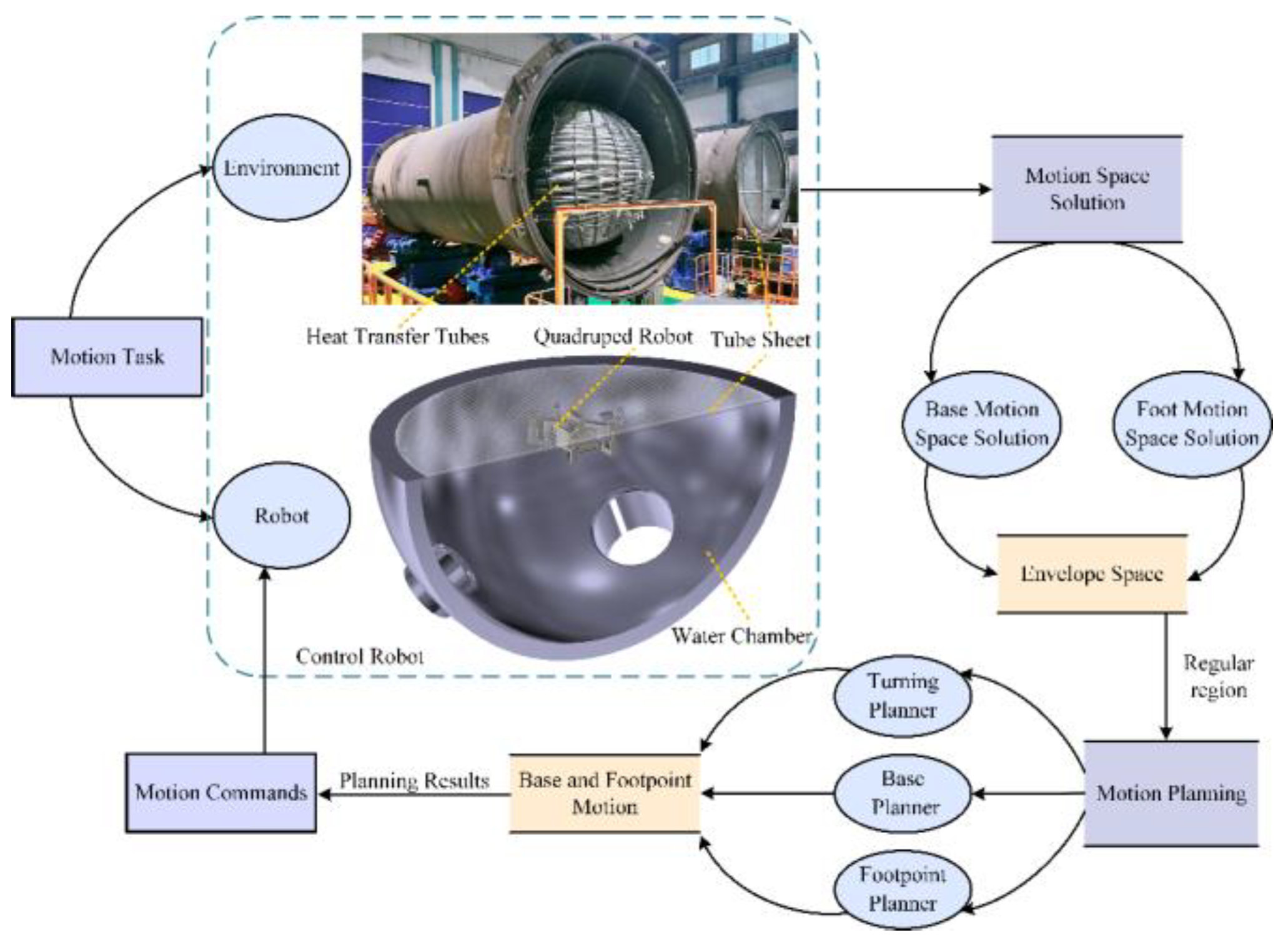
Figure 2.
The structure of HIT_Spibot. (a) The motion modules; (b) and (c) denote the robot with four supporting feet.
Figure 2.
The structure of HIT_Spibot. (a) The motion modules; (b) and (c) denote the robot with four supporting feet.
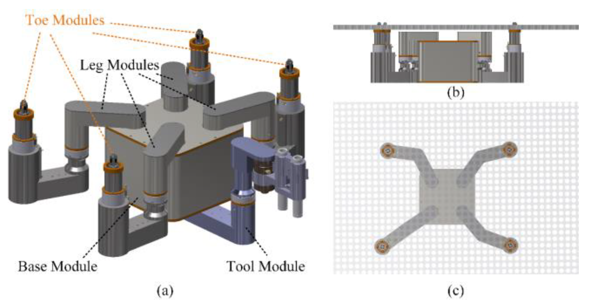
Figure 3.
The coordinate system of HIT_Spibot.
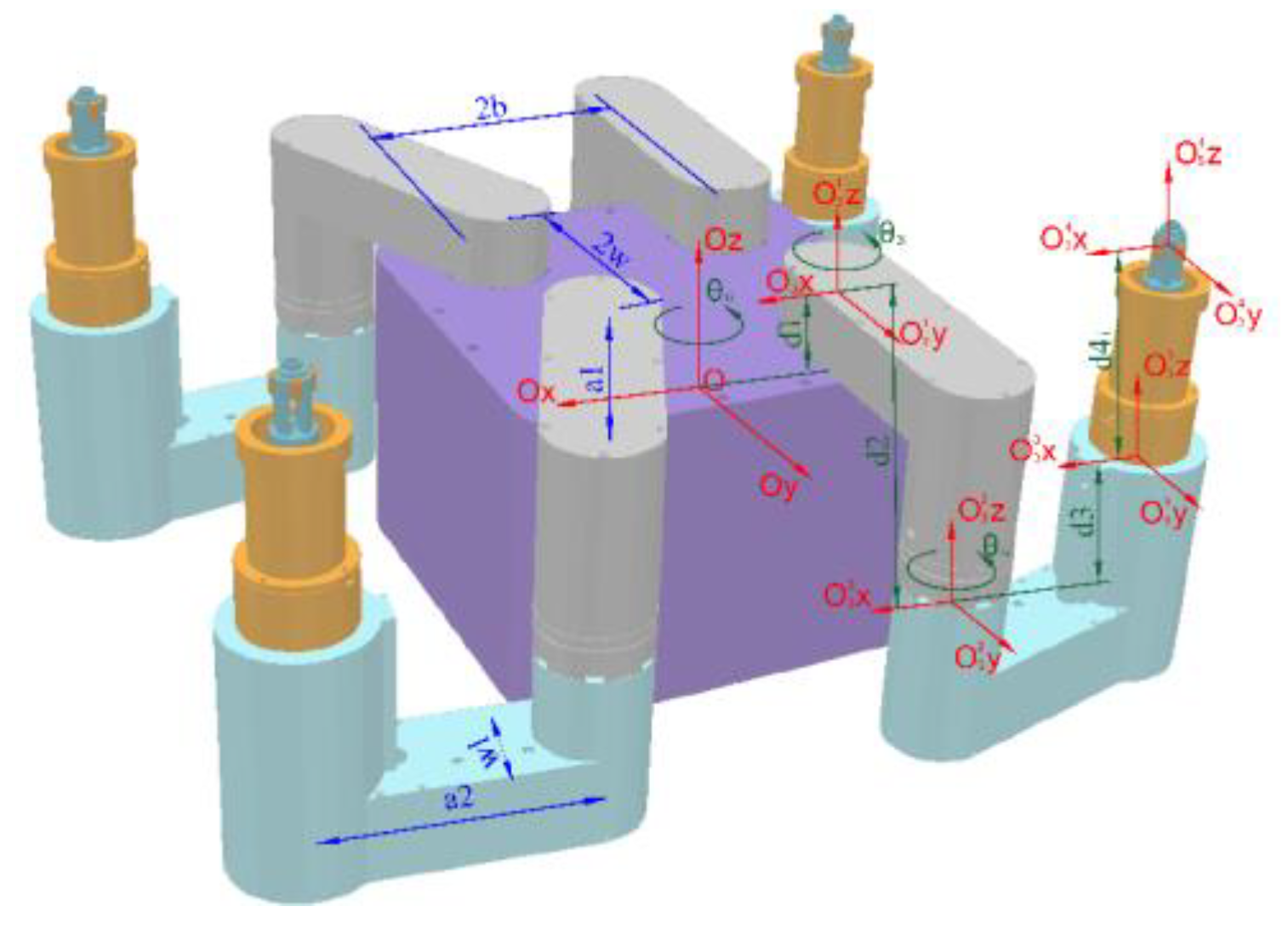
Figure 4.
The motion of the robot base and foot. (a) 2R manipulator arm under three supporting feet; (b) 4-RRR parallel robot under four supporting feet; (c) 3-RRR parallel robot under three supporting feet.
Figure 4.
The motion of the robot base and foot. (a) 2R manipulator arm under three supporting feet; (b) 4-RRR parallel robot under four supporting feet; (c) 3-RRR parallel robot under three supporting feet.
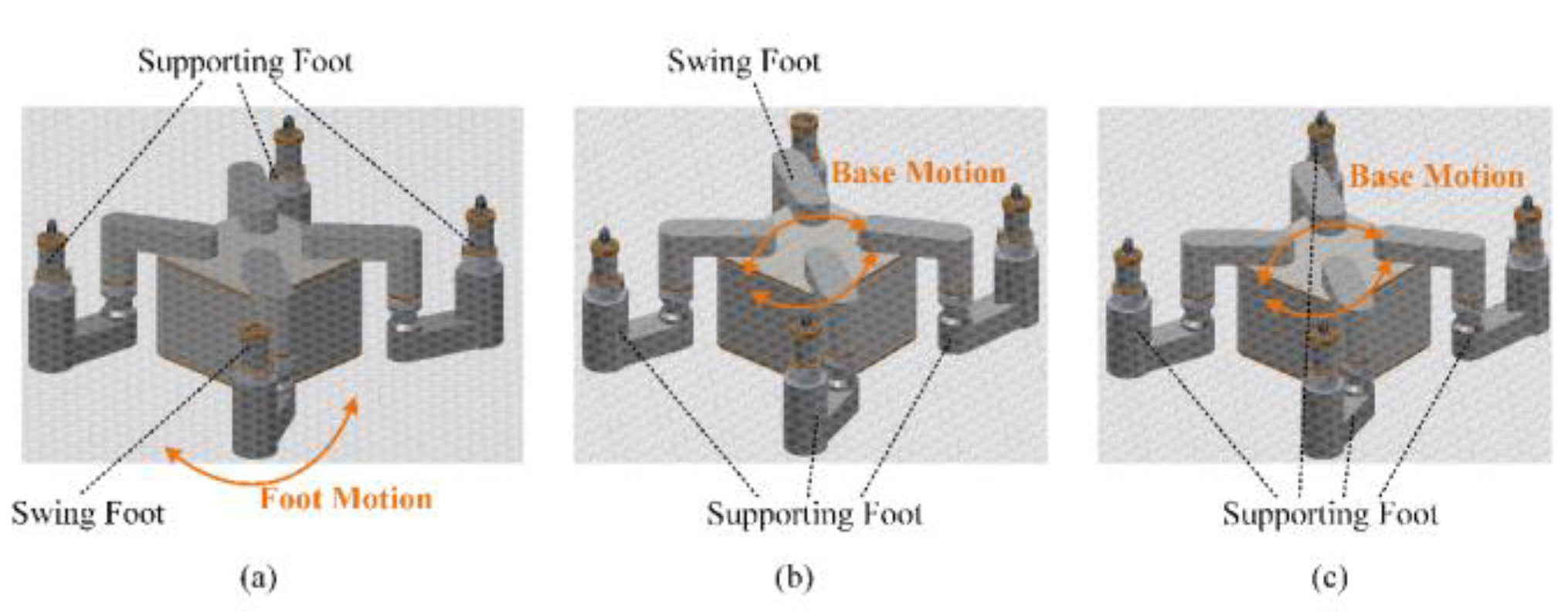
Figure 5.
The workspace of the robot base and feet. (a) The robot feet workspace under the Monte Carlo Method; (b) The boundaries of the workspace. The solid black circles represent the centroids of the circular arcs defining the base workspace, while the red circles represent the centroids of the circular arcs defining the feet’s motion space; (c) The robot base workspace under the Monte Carlo Method.
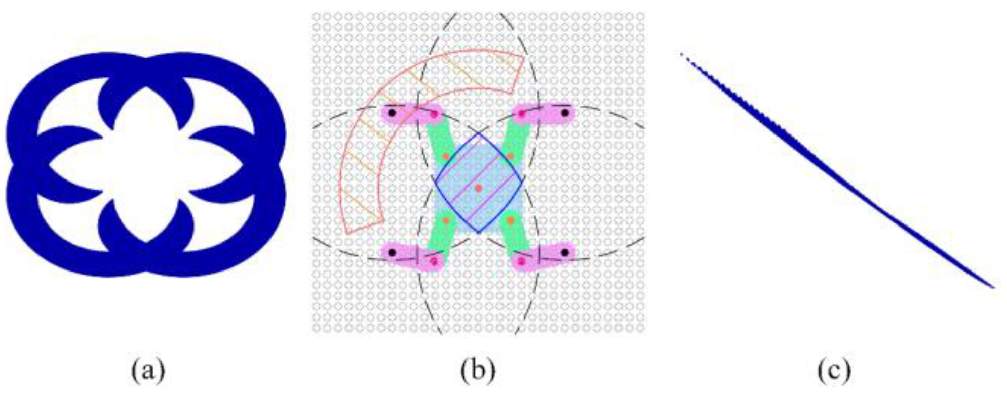
Figure 6.
Workspace envelope rectangles. (a) The swing foot’s envelope rec-tangle and the base’s envelope rectangle under three supporting feet; (b) The swing foot’s envelope rectangle and the base’s envelope rectangle under four supporting feet.
Figure 6.
Workspace envelope rectangles. (a) The swing foot’s envelope rec-tangle and the base’s envelope rectangle under three supporting feet; (b) The swing foot’s envelope rectangle and the base’s envelope rectangle under four supporting feet.
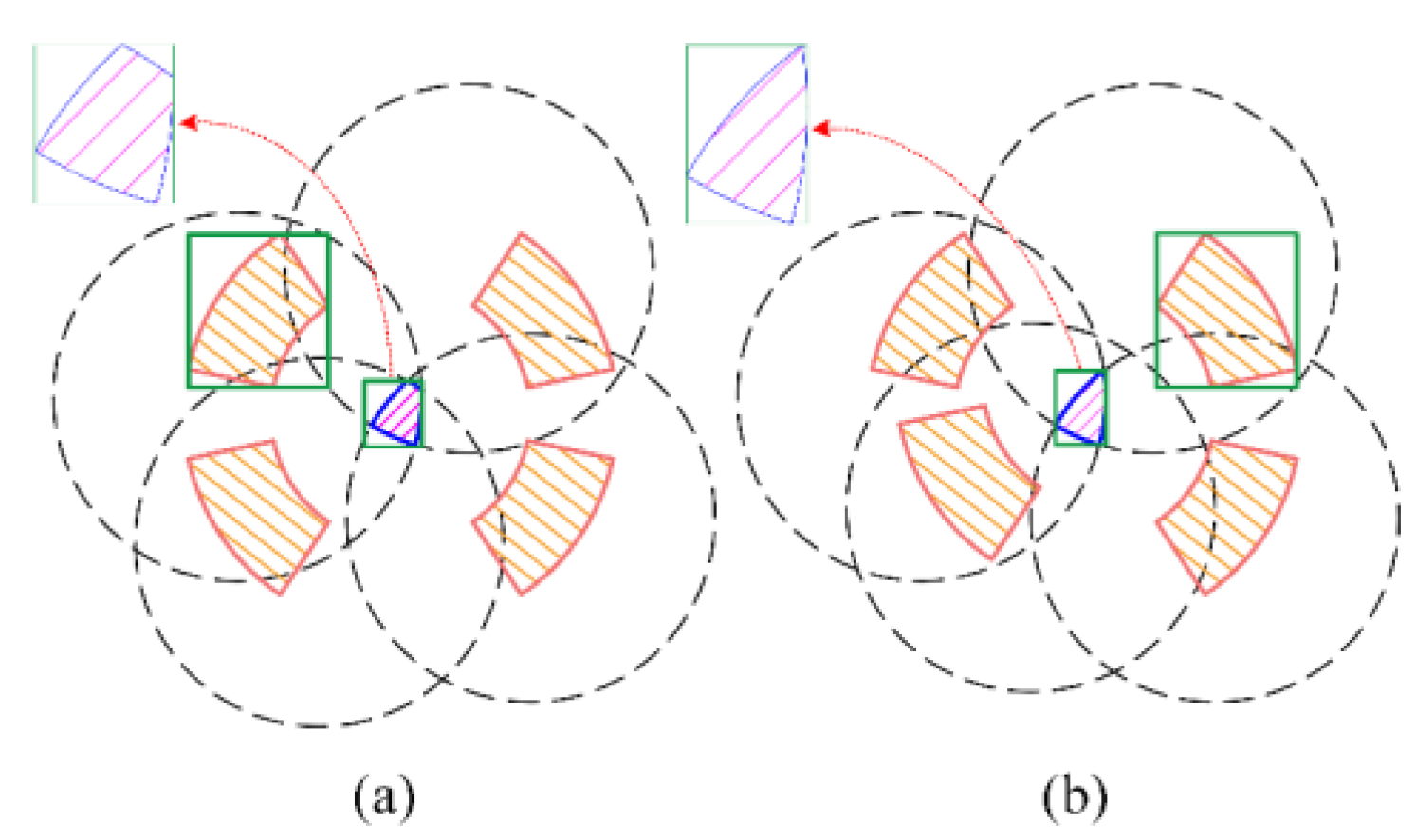
Figure 7.
The evaluation system of the base turning motion.
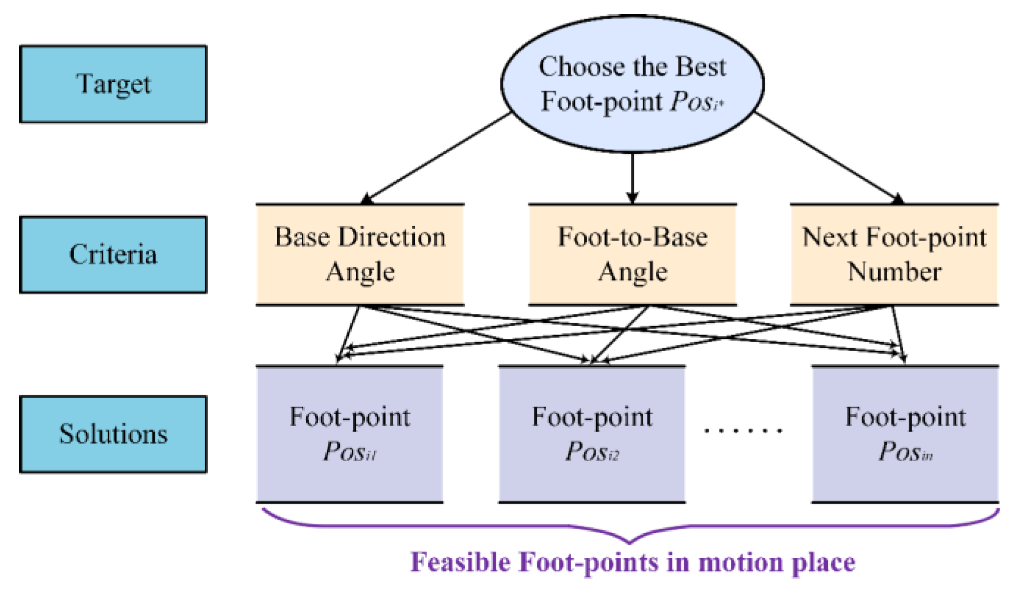
Figure 8.
The foot-point sequence of HIT_Spibot. Arrows indicate the direction of motion for the feet or the base.
Figure 8.
The foot-point sequence of HIT_Spibot. Arrows indicate the direction of motion for the feet or the base.
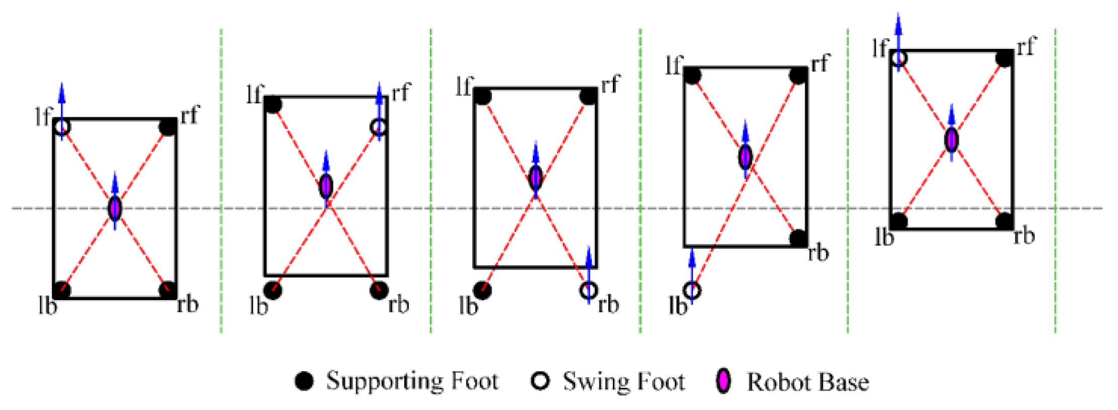
Figure 9.
This is a figure. Schemes follow the same formatting.
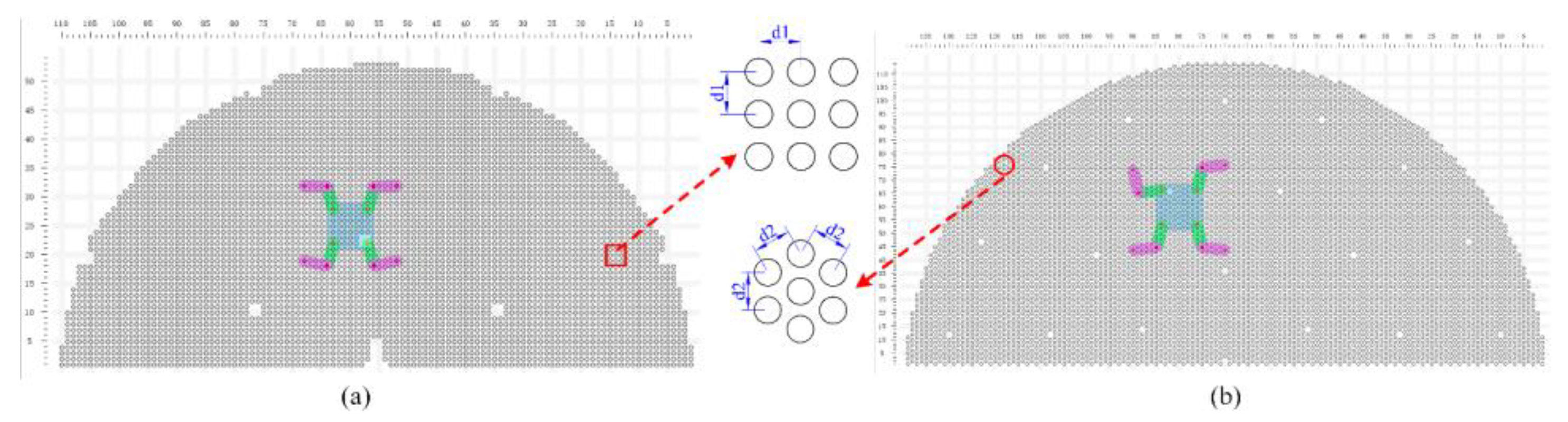
Figure 10.
The robot HIT_Spibot and the real experimental tube plate. (a) HIT_Spibot. (b) the square-distributed tube plate. Due to the large size of the tube plate, the tube plate is taken with a wide-angle camera, which looks like an irregular curved tube plate, but is actually a rectangular tube plate. The orange circles are randomly added obstructed tube holes.
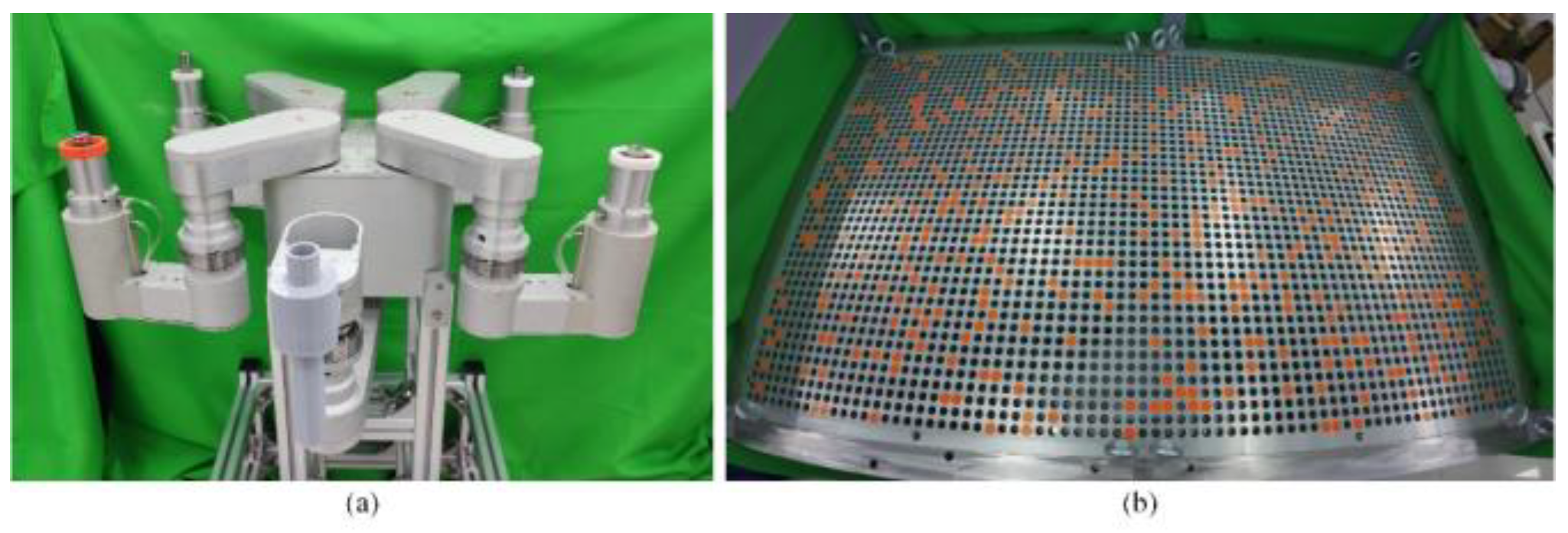
Figure 11.
Average Episode Reward and Step during the training. (a) Average Episode Reward of S-1 (b) Average Episode Step of S-1(c) Average Episode Reward of T-1 (d) Average Episode Step of T-1.
Figure 11.
Average Episode Reward and Step during the training. (a) Average Episode Reward of S-1 (b) Average Episode Step of S-1(c) Average Episode Reward of T-1 (d) Average Episode Step of T-1.
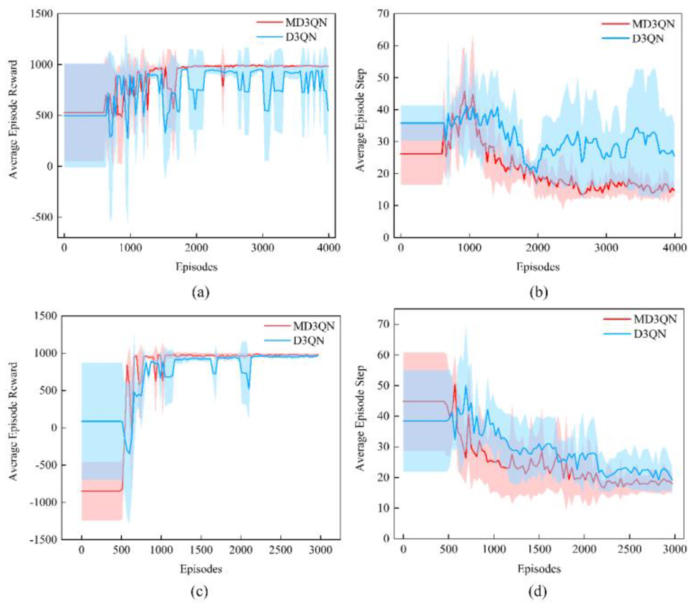
Figure 12.
The task and environment of the performance environment. S1_E4, 5_121 denote task 1 and obstacles environment 4 under square tube plate, the maximum step , and the action space s .
Figure 12.
The task and environment of the performance environment. S1_E4, 5_121 denote task 1 and obstacles environment 4 under square tube plate, the maximum step , and the action space s .
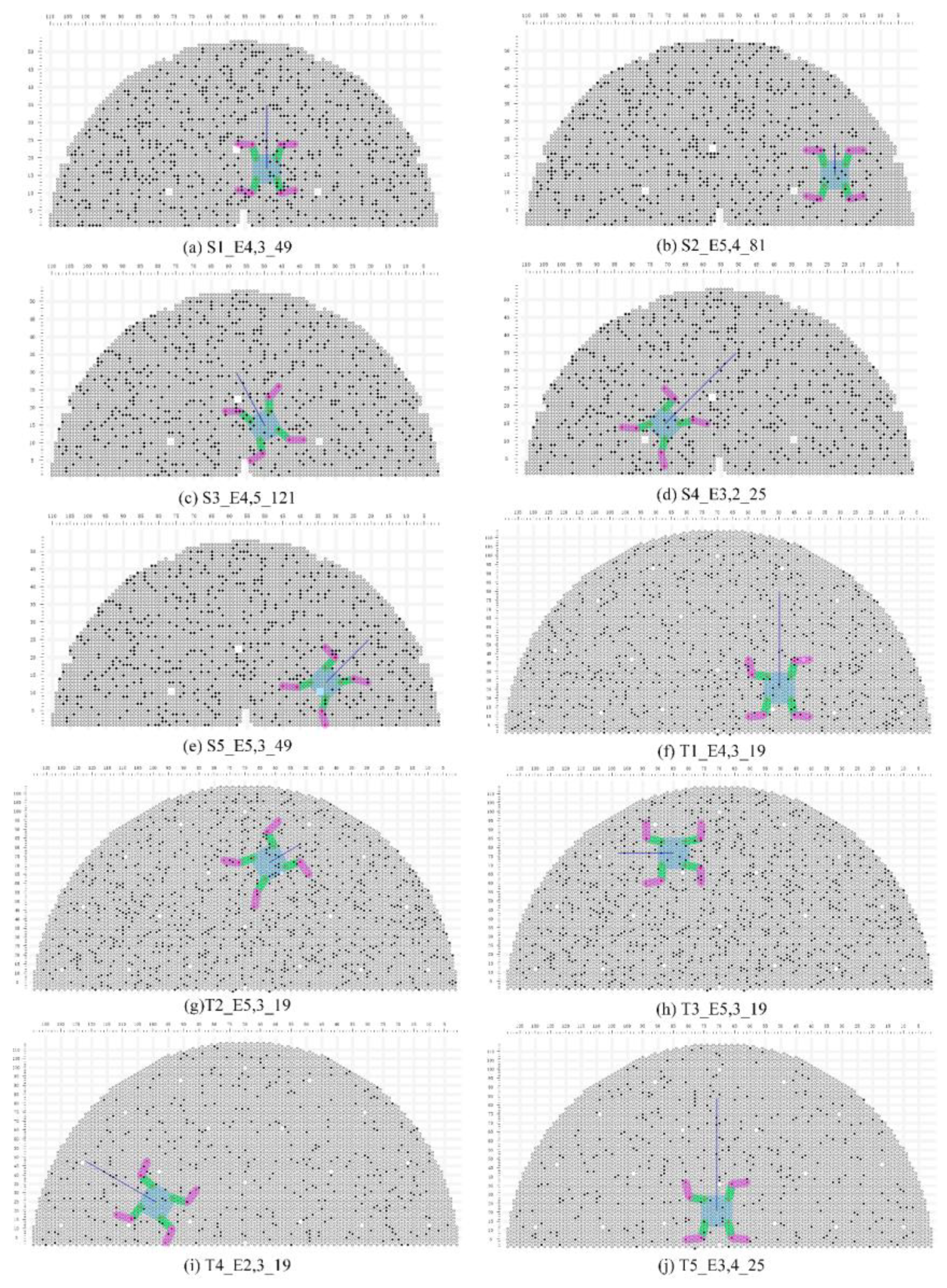
Figure 13.
Simulation and practical comparison of the robot's movement on the tube plate. (a) The initial state. (b) The robot reaches the end of the first segment of the path. (c) The robot turns. (d)-(e) The robot moves along the second segment of the path. (f) The robot reaches the target.
Figure 13.
Simulation and practical comparison of the robot's movement on the tube plate. (a) The initial state. (b) The robot reaches the end of the first segment of the path. (c) The robot turns. (d)-(e) The robot moves along the second segment of the path. (f) The robot reaches the target.
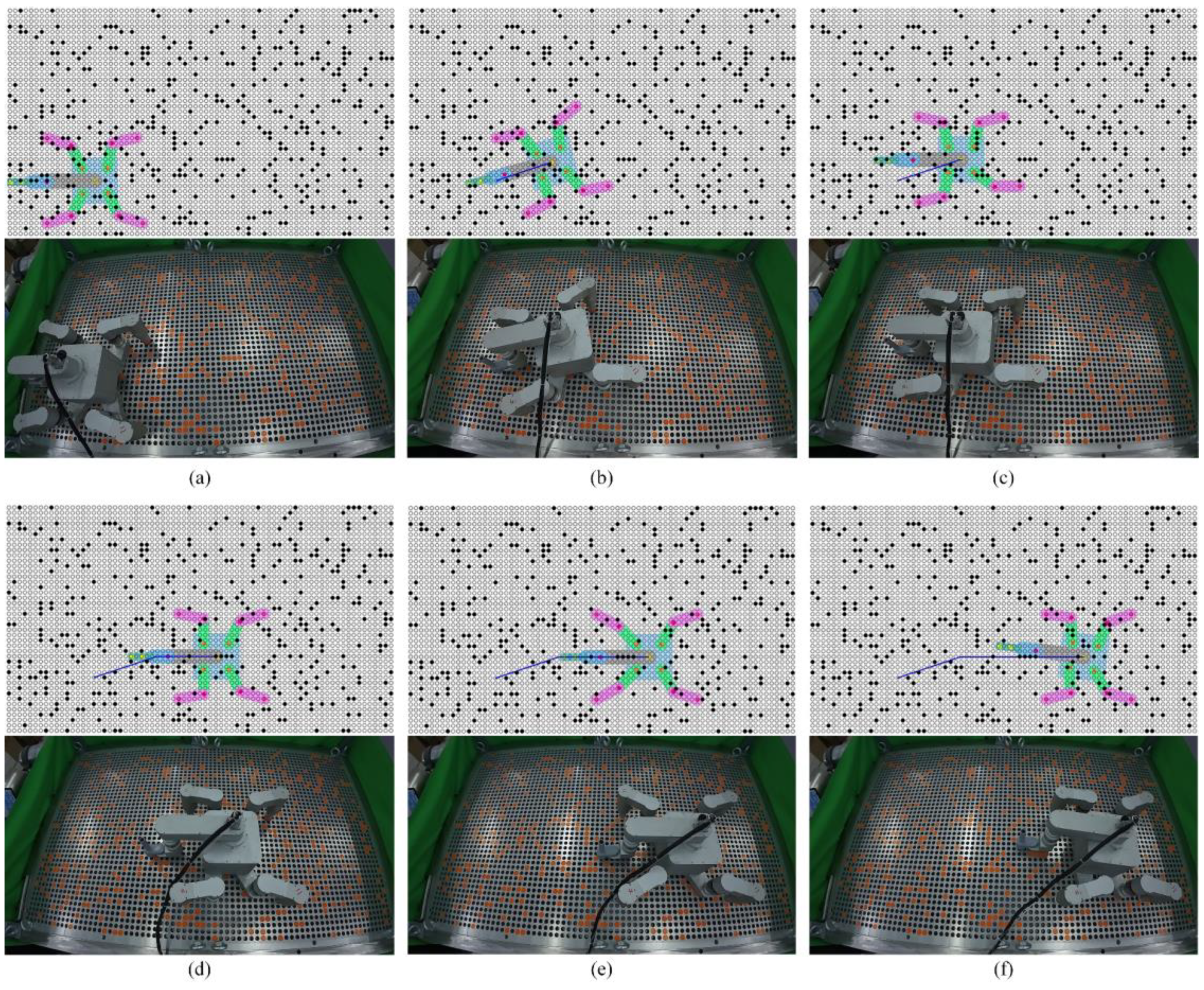

Table 1.
The DH Table of HIT_Spibot.
| Link i | Link length | Joint Twist Angle | Joint distance | Joint angle |
|---|---|---|---|---|
| 1 | 0 | |||
| 2 | 0 | |||
| 3 | 0 | |||
| 4 | 0 | 0 | 0 |
Table 2.
The hyperparameters of the D3QN algorithm.
| Parameter | ||||||||||||||||
| Value | 1e4 | 64 | 0.99 | 50 | 2e4 | 0.05 | 150 | 1e6 | 0.05 | 0.6 | 1.3 | 0.5 | 0.5 | 2 | 1.1 |
Table 3.
The parameters determined by the environment and task.
| 1、2 | 3000 | -1 | 2 |
| 3、4 | 3500 | -1.5 | 3 |
| 5、6 | 4000 | -2 | 3.5 |
| 7、8 | 5000 | -3 | 4.5 |
Table 4.
Robot structure size and motion limitation.
| Parameter | |||||
| Value | 130 | 130 | 130 | 130 |
Table 5.
The training results of the MD3QN and D3QN algorithms.
| E-T | Reward | Step | Stable Reward | |||
|---|---|---|---|---|---|---|
| MD3QN | D3QN | MD3QN | D3QN | MD3QN | D3QN | |
| S-1 | 1004.03 | 982.02 | 13 | 17 | -15.10 | -44.95 |
| S-2 | 977.54 | 914.51 | 13 | 21 | -21.17 | -67.55 |
| S-3 | 986.61 | 951.84 | 10 | 17 | -23.96 | -36.66 |
| S-4 | 993.84 | 965.29 | 14 | 22 | -27.34 | -50.67 |
| S-5 | 1002.91 | 902.81 | 14 | 34 | -18.99 | -118.67 |
| T-1 | 1004.89 | 934.58 | 13 | 25 | -21.86 | -86.863 |
| T-2 | 977.22 | 882.36 | 18 | 36 | -55.84 | -156.64 |
| T-3 | 946.35 | 929.30 | 31 | 33 | -82.23 | -109.07 |
| T-4 | 1007.53 | 959.55 | 17 | 25 | -27.45 | -74.69 |
| T-5 | 965.71 | 871.77 | 17 | 39 | -43.69 | -93.72 |
Table 6.
The performance experiment results of the MD3QN and D3QN algorithms.
| E-T | Metrics | E1 | E2 | E3 | E4 | E5 | |||||
|---|---|---|---|---|---|---|---|---|---|---|---|
| MD3QN | D3QN | MD3QN | D3QN | MD3QN | D3QN | MD3QN | D3QN | MD3QN | D3QN | ||
| S-1 | ASR | 100% | 100% | 100% | 100% | 100% | 100% | 100% | 0% | 100% | 100% |
| AER | 984.02 | 971.53 | 995.09 | 940.93 | 969.76 | 954.34 | 920.56 | — | 1002.51 | 990.43 | |
| AES | 18 | 21 | 20 | 30 | 29 | 30 | 33 | — | 12 | 17 | |
| AESR | -48.05 | -56.15 | -37.24 | -104.85 | -71.42 | -101.67 | -96.10 | — | -15.12 | -31.84 | |
| S-2 | ASR | 100% | 100% | 100% | 100% | 100% | 100% | 100% | 100% | 100% | 0% |
| AER | 977.54 | 858.84 | 963.18 | 913.56 | 941.15 | 845.13 | 858.79 | 745.11 | 970.70 | — | |
| AES | 13 | 34 | 14 | 24 | 27 | 40 | 46 | 54 | 13 | — | |
| AESR | -21.17 | -67.55 | -36.14 | -65.76 | -68.38 | -153.26 | -117.93 | -247.79 | -35.06 | — | |
| S-3 | ASR | 100% | 100% | 100% | 100% | 100% | 0% | 100% | 100% | 100% | 100% |
| AER | 941.96 | 931.67 | 919.98 | 918.90 | 933.56 | — | 858.00 | 608.24 | 946.08 | 935.84 | |
| AES | 19 | 20 | 19 | 24 | 21 | — | 40 | 82 | 17 | 19 | |
| AESR | -55.59 | -57.67 | -72.54 | -78.14 | -68.72 | — | -135.01 | -322.58 | -39.23 | -60.69 | |
| S-4 | ASR | 100% | 0% | 100% | 100% | 100% | 100% | 100% | 100% | 100% | 0% |
| AER | 995.52 | — | 986.30 | 874.38 | 944.49 | 566.69 | 973.55 | 757.92 | 969.32 | — | |
| AES | 13 | — | 22 | 44 | 62 | 139 | 28 | 76 | 28 | — | |
| AESR | -26.39 | — | -50.67 | -164.50 | -139.56 | -585.64 | -60.94 | -308.23 | -70.51 | — | |
| S-5 | ASR | 100% | 100% | 100% | 100% | 100% | 0% | 100% | 0% | 100% | 100% |
| AER | 989.34 | 874.92 | 994.63 | 633.28 | 881.29 | — | 915.64 | — | 964.36 | 660.56 | |
| AES | 12 | 41 | 22 | 92 | 67 | — | 55 | — | 32 | 93 | |
| AESR | -37.97 | -146.84 | -52.99 | -454.45 | -247.05 | — | -194.46 | — | -105.93 | -436.95 | |
| T-1 | ASR | 100% | 100% | 100% | 100% | 100% | 0% | 100% | 100% | 100% | 100% |
| AER | 1006.39 | 915.66 | 1007.55 | 983.56 | 1003.95 | - | 993.08 | 890.05 | 986.48 | 973.93 | |
| AES | 21 | 36 | 17 | 25 | 25 | - | 37 | 6 | 9 | 12 | |
| AESR | -34.15 | -124.38 | -27.41 | -49.89 | -40.70 | - | -94.05 | -190.03 | -27.61 | -45.92 | |
| T-2 | ASR | 100% | 100% | 100% | 100% | 100% | 100% | 100% | 100% | 100% | 100% |
| AER | 976.20 | 882.36 | 952.88 | 771.43 | 934.07 | 702.06 | 982.77 | 901.42 | 832.58 | 820.29 | |
| AES | 18 | 36 | 24 | 61 | 33 | 81 | 9 | 29 | 57 | 60 | |
| AESR | -56.84 | -156.64 | -84.36 | -288.60 | -118.52 | -367.11 | -29.12 | -133.83 | -204.70 | -219.68 | |
| T-3 | ASR | 100% | 100% | 100% | 100% | 100% | 100% | 100% | 100% | 100% | 100% |
| AER | 943.30 | 911.81 | 869.51 | 850.48 | 821.34 | 770.12 | 872.00 | 844.32 | 895.76 | 892.82 | |
| AES | 30 | 38 | 54 | 56 | 83 | 81 | 57 | 59 | 45 | 45 | |
| AESR | -87.83 | -123.91 | -185.78 | -208.67 | -250.32 | -332.46 | -183.42 | -226.92 | -150.42 | -153.60 | |
| T-4 | ASR | 100% | 100% | 100% | 0% | 100% | 0% | 100% | 0% | 100% | 100% |
| AER | 973.07 | 948.82 | 1005.14 | — | 609.85 | — | 842.27 | — | 834.7 | 573.73 | |
| AES | 21 | 25 | 33 | — | 138 | — | 64 | — | 94 | 146 | |
| AESR | -65.12 | -83.55 | -56.45 | — | -552.60 | — | -233.17 | — | -277.48 | -606.02 | |
| T-5 | ASR | 100% | 0% | 100% | 100% | 100% | 100% | 100% | 0% | 100% | 100% |
| AER | 962.06 | — | 846.25 | 712.74 | 895.50 | 422.69 | 711.85 | — | 957.11 | 770.64 | |
| AES | 21 | — | 37 | 67 | 40 | 131 | 73 | — | 16 | 50 | |
| AESR | 37.26 | — | -151.82 | -204.49 | -134.45 | -481.98 | -254.75 | — | -44.53 | 188.02 | |
Disclaimer/Publisher’s Note: The statements, opinions and data contained in all publications are solely those of the individual author(s) and contributor(s) and not of MDPI and/or the editor(s). MDPI and/or the editor(s) disclaim responsibility for any injury to people or property resulting from any ideas, methods, instructions or products referred to in the content. |
© 2024 by the authors. Licensee MDPI, Basel, Switzerland. This article is an open access article distributed under the terms and conditions of the Creative Commons Attribution (CC BY) license (http://creativecommons.org/licenses/by/4.0/).
Copyright: This open access article is published under a Creative Commons CC BY 4.0 license, which permit the free download, distribution, and reuse, provided that the author and preprint are cited in any reuse.


