
Submitted:
30 August 2024
Posted:
02 September 2024
You are already at the latest version
Abstract
In today’s data-driven marketing landscape, accurately predicting customer responses to marketing campaigns is critical for optimizing engagement and return on investment (ROI). This study utilizes a Decision Tree (DT) model to identify key factors influencing customer behaviour. Initially, the model achieved a high accuracy of 87.3% but struggled with precision and recall due to class imbalance. By applying a resampling technique, the model’s performance improved significantly, with a recall increase from 44% to 83.1% and an F1-score improvement from 49% to 74.2%. Key influential features identified include how recently a customer made a purchase, the number of days they have been a customer, and the number of previous campaigns they responded to. The study highlights the DT model’s interpretability, making it a practical tool for marketing professionals to improve campaign effectiveness and customer targeting.
Keywords:
Customer Relationship Management
; Customer response prediction
; Decision Tree model
; F1-score
; ROI optimization
; Predictive modeling
1. Introduction
In today’s highly competitive and data-driven business environment, understanding customer behaviour is crucial for effective marketing strategies [1]. Predicting how customers will respond to marketing campaigns not only improves the effectiveness of these efforts but also significantly increases ROI [2]. As companies gather vast amounts of data from various customer touchpoints, the challenge is transforming this data into actionable insights for targeted and personalized marketing. Predictive modelling, particularly using DT models, offers a promising solution by using historical data to forecast future customer behaviour [3]. Marketing strategies can be divided into mass marketing and direct marketing. Mass marketing uses widespread media platforms like television, and radio, to reach existing and potential customers. In contrast, direct marketing focuses on contacting specific clients directly, often proving more cost-effective and resource-efficient. Understanding the effectiveness of these strategies requires a deep understanding of customer behaviour. A paper by Raorane and Kulkarni [4] suggests that studying consumer psychology, mindset, behaviour, and motivation allows companies to refine their marketing strategies. Therefore, collecting and analyzing customer data is essential for businesses. Customer Relationship Management (CRM) allows for the automatic collection of this data, which includes demographics, purchase history, and interactions with the company. This field revolves around identifying, establishing, and sustaining long-term relationships with clients. Utilizing CRM data is crucial for informed marketing decisions [5]. Traditionally, customer behaviour prediction relied on managers’ intuition and experience, with decisions based on general trends rather than analytical support. However, the rise of Machine Learning (ML) has transformed predictive analytics, leading to the development of more advanced models. Tree-based ML classifiers, such as DT and Random Forest (RF) models, are known for their high accuracy and interpretability. DT models are particularly favored for their ease of understanding and visualization [3], as they create a tree-like structure of decisions based on input features. RFs, on the other hand, are an ensemble method that improves the predictive power of DT by aggregating the results of multiple trees, improving generalization, and reducing overfitting, meaning preventing the model from becoming too finely tuned to the training data[6]. The question of whether RF outperforms DT in predicting customer marketing responses is multi-dimensional. However, an advantage of both models is their capability to assess feature importance. This analysis can identify the most influential factors in predicting customer responses to promotions and marketing campaigns. By determining which customer attributes have the greatest impact, businesses can tailor their strategies and allocate resources more effectively. While the RF method is more robust against noisy data compared to just using a single DT[6,7], when the dataset is relatively small, and the interpretability of the model is crucial, DT is the better choice. They are easier to interpret than RF, due to their representation of simple decision rules, making it easier to understand how each feature contributes to the model’s predictions[8]. Despite the potential of predictive modelling, businesses often face significant difficulties in accurately predicting customer responses to marketing campaigns. The complexity of customer behaviour, influenced by many factors such as demographics and past interactions, makes it difficult to develop reliable models. Traditional approaches tend to overlook these complexities, leading to generalized and less effective marketing strategies [5]. This study seeks to address this gap by focusing on the interpretability and explainability of the predictive model, by utilizing the DT algorithm [3]. The primary objective is to identify and understand the most influential demographic factors, such as age, income, marital status, and education level, as well as examine the impact of past interactions with the company, including previous purchases and engagement with earlier campaigns. The research aims to achieve this through the following questions:
- RQ1
- What are the challenges and limitations presented in the literature regarding predicting customer marketing responses?
- RQ2
- How effective is the DT model at predicting customer response to marketing campaigns?
- RQ3
-
What are the key factors influencing customer response to marketing campaigns as identified by the DT model?
- –
- Which demographic factors are most influential in predicting customer response to marketing campaigns according to the DT model?
- –
- How do past interactions with the company affect future responses according to the DT model?
The rest of the paper is organized as follows: Section 2 reviews related work, discussing existing literature and the performance of DTs in predictive analytics. The methodology and practical implementation are detailed in Section 3, while Section 4 presents the research findings. Section 5 discusses the results and their implications, and Section 6 concludes with a summary of key findings, limitations, and directions for future research.
2. Related Work
This section reviews key studies that investigate the application of various predictive models in direct marketing, highlighting their methodologies and results. A paper by K. Wisaeng [9] compares different classification techniques in bank direct marketing, using a UCI repository data set with 16 attributes and 45,211 instances. The study examines two decision tree methods, J48-graft and LAD tree, and two machine learning approaches, Radial Basis Function Network (RBFN) and Support Vector Machine (SVM). The results indicate that among the algorithms tested, the SVM outperformed others, achieving the highest accuracy of 86.95%. In contrast, the RBFN showed the least effective performance with an accuracy of 74.34% [9]. Research by Sérgio Moro et al. [10] applied Logistic Regression (LR), Neural Networks (NN), DT, and SVM on a dataset sourced from a Portuguese bank, including 22 selected features. Their study highlighted the performance of the NN in predicting customer behaviour. To optimize marketing strategies the study provided practical insights, revealing that targeting the top half of customers classified as more likely to respond positively could lead to successful outcomes in 79% of cases. Suggesting that a selective approach to customer engagement can potentially reduce costs while maximizing campaign efficiency [10]. Another paper by Sérgio Moro [11] applied different data mining algorithms such as Naive Bayes (NB), DT, and SVM. The findings indicated that SVM has the highest prediction performance, with NB and DT following. The call duration was found to be the most significant feature, followed by the month of contact. DTs have emerged as a fundamental tool in predictive analytics for marketing. By offering a transparent and interpretive model, DTs provide marketers with valuable insights into the influence of different customer attributes on marketing outcomes [3,8]. Many studies underscore the potential of DT models as a powerful tool for businesses seeking to optimize their marketing strategies and maximize customer engagement. The study conducted by authors in [12] demonstrated the effectiveness of DT models in forecasting customer responses to direct marketing. The researchers utilized DT models to analyze historical data from various marketing campaigns, to predict future customer behaviour. The DT models were trained on a range of features, including demographic information and past interactions with the company. Among the customers who were predicted not to respond to direct marketing, the model’s accuracy was 87.23%. This means that in 87.23% of cases, the customers who were predicted not to respond indeed did not respond [12]. On the other hand, among the customers who were predicted to respond to direct marketing, the model’s accuracy was 66.34%. This indicates that in 66.34% of cases, the customers who were predicted to respond did indeed respond [12]. Another study conducted on customer churn analysis for live stream e-commerce platforms used DT, Naive Bayes, and K-nearest neighbour algorithms to classify customers into churners and non-churners groups. The DT algorithm outperformed the other models with an accuracy of 93.6%. A similar research by Usman-Hamza et al. [13] highlighted the effectiveness of tree-based classifiers in customer churn prediction, outperforming other forms of classifiers in most cases. The RF ensemble arguably increases the generalization accuracy of Decision Tree-based classifiers without trading away accuracy on training data[14]. As per Chaubey et al. [1], this suggestion translates into the problem of customer purchasing behaviour prediction. Their paper suggests that when comparing the accuracy of models for churn prediction, RF has been found to perform better than the DT model, suggesting its potential to improve accuracy in specific predictive tasks. However, a study by Apampa [15] examines to what extent the use of RF ensemble improves the performance of the DT classification algorithm for the bank customer marketing response prediction. In this study it was concluded that the use of RF ensemble does not improve or improve the performance of the DT algorithm, suggesting that RF might not consistently improve DT’s performance, particularly in contexts such as predicting bank customer responses to marketing. Additionally, interpreting the resulting RF model remains a challenging task, as even machine learning experts struggle to precisely analyze and uncover the detailed predictive structure [6]. Making the DT algorithm the most appropriate when interpretability is favored. Previous research has primarily focused on applying various ML techniques and comparing their efficiency. However, there has been a notable gap regarding the treatment of complexity issues. Decision-makers with limited technical backgrounds often struggle to grasp the complex relationships between attributes in traditional ML models. Therefore, this study aims to address this gap by applying a straightforward DT model that is easy to interpret. Table 9 summarizes the different models used, their accuracy, and key findings from each study.
3. Proposed Solution
This research follows a six-stage methodology that is designed to be straightforward and interpretable for individuals with a moderate understanding of data mining. The whole procedure is shown in Figure 1:

Table 1.
Benchmark of Related Work in Predictive Models for Direct Marketing.
| Study | Models Compared | Best Accuracy Achieved | Key Findings |
|---|---|---|---|
| K. Wisaeng [9] | SVM, J48-graft, LAD tree, RBFN | 86.95% (SVM) | SVM outperformed other models, RBFN had the lowest accuracy. |
| Sérgio Moro et al. [10] | Logistic Regression, Neural Networks, Decision Tree, SVM | 79% (Neural Networks) | Neural Networks performed best in predicting customer behavior; targeting top half of customers improved outcomes. |
| Sérgio Moro [11] | Naive Bayes, Decision Tree, SVM | N/A (SVM) | SVM showed the highest prediction performance, with call duration as the most significant feature. |
| Choi et al. [12] | Decision Tree | 87.23% (Non-responders) | Decision Tree accurately predicted non-responders but had lower accuracy for predicting responders. |
| Usman-Hamza et al. [13] | Decision Tree, Naive Bayes, K-nearest neighbor | 93.6% (Decision Tree) | Decision Tree outperformed other models in customer churn analysis for live stream e-commerce. |
| Chaubey et al. [1] | Random Forest, Decision Tree | N/A (Random Forest) | Random Forest performed better than Decision Tree for churn prediction but lacks interpretability. |
| Apampa [15] | Random Forest, Decision Tree | N/A (Decision Tree) | Random Forest did not consistently improve Decision Tree’s performance in bank marketing prediction, favoring Decision Tree for interpretability. |
3.1. Hardware and Software Configuration
The hardware and software configuration for this research ensures the reproducibility of the experiment. In Table 2 are listed the specific components and tools used. To ensure transparency and accessibility in the research process, the source code for this research is made publicly available in a GitHub repository1.
3.2. Data Collection
The dataset used in this study was obtained from the online platform Kaggel and it belongs to the Brazilian food ordering platform iFood [16]. As presented in Table 3 it includes various demographic data, such as age, income, marital status, and education level. As well as customer interaction data, such as previous purchases and previous marketing responses. The total number of instances is 2206. The dataset consists of 39 attributes, with the target variable ’Response’ being a binary indicator. This target variable has two classes, "yes," indicating that the customer responded positively to a marketing campaign, and "no," indicating that the customer responded negatively. Notably, the dataset contains no categorical data. All attributes are either numerical or binary indicators. This structure eliminates the need for encoding categorical variables. However, the target class is imbalanced, highlighting the need for resampling techniques or adjusting class weights to address this issue.
3.3. Model Selection
DT is a supervised ML method, aiming to establish a relationship between input features and the target variable for accurate predictions [3]. Structurally, decision trees resemble a tree where each node signifies a decision based on an attribute, each branch corresponds to an outcome of that decision, and each leaf node represents a target class label. The classification process involves tracing a path from the root node, the primary attribute, to a leaf node [3]. This intuitive method uses an "if-else" logic, making it straightforward to understand and interpret [3,8]. This is especially useful in marketing, where decisions are often made by individuals with limited technical knowledge, making decision trees an appropriate choice.
3.4. Data Preprocessing
It is observed that the dataset is significantly imbalanced, with a considerably higher number of negative responses ("no") compared to positive responses ("yes"). This class imbalance poses a notable challenge because the model tends to predict the majority class more frequently. While this may lead to high overall accuracy, it results in poor identification of the minority class, which is crucial for the campaign’s success [17]. To address the issue of class imbalance, a technique called resampling is implemented. Resampling involves adjusting the dataset to balance the class distribution, ensuring that the model has an equal representation of both classes during training. This can be achieved through various methods such as oversampling the minority class or undersampling the majority class [17]. In this study, the undersampling technique is applied. This approach involves decreasing the number of instances in the majority class (negative responses) to match the number of instances in the minority class (positive responses), resulting in a more balanced dataset that allows the model to learn the characteristics of both classes more effectively. In addition to resampling, another effective approach that is used is adjusting the class weights [17]. By assigning higher weights to the minority class, the model further improves its sensitivity towards positive responses [18].
3.5. Model Development
In the next part of the research, the DT model is developed using a structured and methodical approach. Initially, the dataset is prepared, by partitioning the features into predictors (X) and the target variable (y). This method ensures that the model learns to predict the target variable based on the features [19]. The predictors consist of everything except the ’Response’ column, which serves as the target variable. The dataset is divided into training and testing sets with an 80-20 ratio, meaning 80% of the data is used to train the model, and the remaining 20% is used to test it. This partitioning allows for the evaluation of the model’s performance on unseen data, which simulates real-world scenarios where the model will encounter new data. This way the model generalizes well and is not overfitted to the training data [19]. Additionally, a random state of 42 is specified to guarantee reproducibility of the results, ensuring that the random processes involved in data splitting will produce the same results every time the code is run.
3.5.1. Hyperparameter-tuning
After resampling, a grid search method, combined with cross-validation, is applied to explore different combinations of hyperparameters. One of the key ones is the ’criterion,’ which determines the function used to measure the quality of a split. The options for the ’criterion’ parameter include Gini impurity and entropy [19]. Gini impurity is defined in Equation 1:
Where represents the proportion of instances belonging to class i in the dataset. Gini impurity measures the probability of incorrectly classifying a randomly chosen element. An impurity of 0 indicates that all elements in a node belong to a single class, representing perfect purity. In practical terms, a lower Gini impurity means that the DT is better at creating homogeneous groups of customers, which can lead to more accurate predictions.[19]. Entropy is defined in Equation 2:
It measures the amount of disorder within a set of classes. When the entropy is 0, it means there is no disorder, and all customers within a node share the same classification. Higher entropy values indicate greater disorder and less purity. The criterion of entropy often leads to more balanced splits compared to Gini impurity, as it creates splits that increase the information gain, making it a preferred choice when the goal is to achieve higher accuracy and a more informative model [19]. Another important hyperparameter is the ’splitter’. The ’splitter’ can be set to ’best’ or ’random.’ The ’best’ option selects the optimal split among all features, aiming to maximize information gain or minimize Gini impurity. On the other hand, the ’random’ option selects a random feature and then finds the best split within that feature. Parameter ’best’ might result in a more accurate but computationally intensive model, whereas ’random’ can lead to faster training times and increased generalization [19]. The ’max_depth’ parameter controls the maximum depth of the tree. It ranges from no limit, allowing the tree to expand until all leaves are pure, to a specified maximum depth, such as 5, 10, 15, or 20. A shallower tree generalizes better on unseen data, whereas a deeper tree can capture more details from the training data but risks overfitting [19]. The ’min_samples_split’ parameter specifies the minimum number of samples required to split an internal node. It ranges from 2 to 15. A higher value prevents the model from learning too much from the noise in the training data, thus improving its generalization capability [19]. Finally, the ’min_samples_leaf’ parameter indicates the minimum number of samples required to be at a leaf node. It ranges from 1 to 6. A higher value can lead to a more generalized model, whereas a lower value might allow the tree to capture more patterns [19]. By conducting an exhaustive grid search across these parameters, the model is evaluated through cross-validation for each combination. This means the model is trained and evaluated on different subsets of the training data to ensure that the hyperparameters are not overfitted to a particular subset. The cross-validation divides the training data into five parts, training the model on four parts and validating it on the fifth, rotating this process to cover all combinations [20]. The best combination of hyperparameters is identified based on the average performance across these folds [20]. The best estimator from the grid search is then selected as the final model (best_clf) for further evaluation.
3.6. Model Evaluation
Evaluating the performance of the predictive model is crucial in understanding how well it generalizes to new, unseen data. In this research, several key metrics are utilized to assess the effectiveness of the DT model in predicting customer responses to marketing campaigns. These metrics include accuracy, precision, recall, F1 score, and the confusion matrix
3.6.1. Confusion Matrix
To gain a comprehensive understanding of a model’s effectiveness in imbalanced scenarios, the use of a confusion matrix is essential. It summarizes the prediction results, showing the count of correct and incorrect predictions broken down by each class. The matrix is structured in Table 4: True Positives (TP) refers to the number of instances where the model correctly predicts a customer will respond positively to a campaign, aligning with actual positive responses. True Negatives (TN) denote cases where the model accurately identifies customers who will not respond, matching the actual negative responses. False Positives (FP), often termed "false alarms," occur when the model incorrectly predicts a positive response from customers who, in reality, do not respond to the campaign. Conversely, False Negatives (FN) happen when the model fails to predict a positive response from customers who indeed respond [21].
3.6.2. Accuracy
Accuracy is a measure of the overall correctness of the model [21], representing the proportion of correctly predicted instances out of the total instances, as shown in Equation 3.
For this model, the accuracy indicates how well it can correctly classify both positive and negative responses. In the case of the imbalanced dataset in this study, high accuracy can be achieved by simply predicting the majority class most of the time. However, this high accuracy is deceptive because the model fails to identify the customers who respond, making it ineffective for practical purposes. The limitations of accuracy in the context of imbalanced datasets highlight the importance of alternative metrics such as precision, recall, and the F1 score [17].
3.6.3. Precision
Also known as positive predictive value. As defined in Equation 4 precision measures the accuracy of positive predictions [21].
In this study, precision indicates the proportion of customers who are predicted to respond positively and indeed did respond positively.
3.6.4. Recall
3.6.5. F1-Score
The F1-score is the harmonic mean of precision and recall, providing a single metric that balances the two. It is particularly useful when there is an uneven class distribution [21]. The formula for the F1-score is shown in Equation 6:
The F1-score ranges from 0 to 1, where 1 indicates perfect precision and recall, and 0 indicates the worst possible performance. This metric is beneficial when seeking a balance between precision and recall, especially in the presence of class imbalance [21].
3.7. Feature Importance Extraction
In this step, feature importance scores are extracted from the trained DT model and the top 10 features are identified and visualized. Feature importance is a metric that indicates the significance of each input variable in contributing to the prediction accuracy of the DT classifier.
3.8. Decision Rules Generation
In this step, the decision tree rules are generated in the form of if.. else statements. They allow for easy interpretation of the decision-making process, where one can understand how a particular prediction is made. The clarity of the DT rules enables stakeholders, who may not have a deep technical background, not only to pinpoint these influential factors accurately but also to utilize them effectively.
4. Results
In this section of the study, the best hyperparameters resulting from the grid search combined with cross-validation are presented before and after resampling is applied. Additionally, a comparative analysis of the model evaluation results before and after resampling is conducted. The analysis focuses on the confusion matrix and various performance metrics, including accuracy, precision, recall, and F1-score, to evaluate the model’s effectiveness. Furthermore, the results include feature importance scores and the generated decision rules, which are extracted from the decision tree classification model after resampling. This approach is taken because the resampled dataset provides a more balanced and accurate representation of the underlying patterns, leading to more reliable and interpretable decision rules and feature importance scores.
4.1. Best Hyperparameters
4.1.1. Before Resampling
The grid search combined with cross-validation identified the optimal hyperparameters to be the ones presented in Table 5 before resampling was applied.
These hyperparameters reflect a conservative approach to handling the significant class imbalance in the dataset. The criterion of entropy helps in maximizing information gain at each split. By limiting the maximum depth to 5, the model avoids overfitting to the majority class of negative responses, which dominates the dataset. The parameters for minimum samples per leaf and split ensure that each node has enough data to make reliable decisions, thus reducing the likelihood of splits based on noise or anomalies. The use of a random splitter adds an element of randomness to the decision-making process, which helps prevent the model from becoming overly complex and biased towards the majority class during training.
4.1.2. After Resampling:
Following the application of undersampling to balance the class distribution, the grid search with cross-validation identified a different set of optimal hyperparameters, presented in Table 6.
The shift in hyperparameters post-undersampling indicates a significant change in the model’s complexity and its approach to decision-making. With the maximum depth set to None, the model is allowed to grow without constraints until all leaves are pure or until they contain fewer samples than the minimum samples split threshold. This unrestricted growth enables the model to capture more detailed patterns in the balanced dataset. The switch to the best splitter means the model now selects the optimal split at each node, based on the entropy criterion, to maximize information gain, leading to more precise and effective splits that better separate the classes.
4.2. Confusion Matrix
4.2.1. Before Resampling
The confusion matrix before resampling is presented in Table 7 and it reveals that the model correctly identifies 27 true positives and 357 true negatives, while there were 21 false positives and 36 false negatives. This indicates that the model was successful in predicting customers who would respond positively to marketing campaigns in 27 instances and correctly identifying customers who would not respond in 357 instances. The high number of true negatives compared to true positives is attributed to the imbalance in the target class ’Response’. The model is exposed to more instances of non-response during training, which makes it better at identifying non-responders (true negatives) but limits its capacity to detect responders (true positives). The model also produced 21 false positives (FP) representing instances where the model incorrectly predicted a positive response from customers who did not respond. Conversely, the 36 false negatives (FN) produced, indicate cases where the model failed to predict a positive response from customers who did respond positively. This means that the model occasionally mistakes non-responders for responders, potentially leading to unnecessary marketing efforts toward those unlikely to engage. More critically, the higher number of false negatives signifies that the model misses many potential customers who would have responded positively, ultimately resulting in missed opportunities for engagement.
4.2.2. After Resampling:
The confusion matrix after resampling is presented in Table 8 and it reveals that the model correctly identifies 49 true positives and 51 true negatives, while there were 24 false positives and 10 false negatives. Post-resampling, the model’s ability to correctly identify positive responses improves significantly, evidenced by the increase in true positives from 27 to 49. This improvement is primarily due to the undersampling technique, which balances the class distribution by reducing the number of majority class instances, thereby allowing the model to learn more effectively from the minority class. However, this adjustment also leads to a slight increase in false positives (from 21 to 24) and a decrease in true negatives (from 357 to 51), as the model now encounters fewer non-responders during training. This trade-off is typical when addressing class imbalance; while the model becomes better at identifying the minority class, it may lose some accuracy in predicting the majority class. Despite this, the drop in false negatives from 36 to 10 is significant, indicating a more balanced and effective model that is better equipped to predict both responders and non-responders.
The breakdown made in the confusion matrix is crucial for calculating the performance metrics.
4.3. Model Evaluation
4.3.1. Before Resampling
The performance of the model before resampling is presented in Figure 2
Despite the high accuracy of 87.3%, the precision, recall, and F1-score are relatively low. Accuracy alone can be misleading in cases of imbalanced datasets, where one class significantly outweighs the other. Here, the high accuracy mainly reflects the model’s ability to correctly identify non-responders, but it does not adequately capture the performance in predicting the responders.
The precision, which is calculated to be 56%, measures the proportion of true positive predictions among all positive predictions. This means that out of all the instances, that the model predicted as responders, only 56% were correct. The recall, calculated to be 44%, measures the proportion of actual positive instances that were correctly identified by the model. This means that the model only identified 44% of the actual responders correctly. The low F1-score reflects the overall inefficiency of the model in handling the imbalanced dataset, as it struggles to achieve a good trade-off between precision and recall. While the model appears to perform well based on accuracy alone, the low precision, recall, and F1-score reveal its limitations in predicting the minority class effectively.
4.3.2. After Resampling:
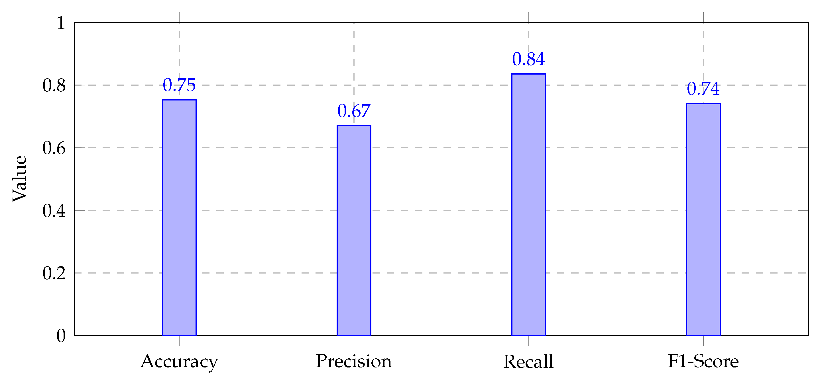
The performance of the model after resampling is presented in Figure 3.
Post-resampling, the model’s performance improved significantly. The accuracy dropped to 74.6%, which is expected as the model now faces a more balanced dataset, making predictions more challenging. However, this decrease in accuracy is not necessarily a negative outcome. The balanced dataset has allowed for improvements in other critical metrics. The precision increased to 67.1%, indicating that the model is now better at correctly identifying true responders, reducing the number of false positives where non-responders are incorrectly predicted as responders. The recall increased to 83.1%, demonstrating a substantial improvement in capturing most of the true positive cases, thereby reducing the number of false negatives where actual responders are missed. Finally, the F1-score improved to 74.2%, providing a balanced measure of the model’s precision and recall. The significant improvement in the evaluation metrics indicates that the model is now well-suited to identify both responders and non-responders accurately, making it more effective for practical applications in marketing campaigns.
Figure 3.
Evaluation metrics after resampling.
4.4. Feature Importance Scores
The top 10 most influential features are presented in Figure 4. Demographic factors such as age and income are reported to play a crucial role in customer behaviour. Past customer interactions with the company, indicated by variables like Recency (days since last purchase), Customer_Days (days since customer registration), and AcceptedCmpOverall (number of accepted campaigns), are significantly influential to customer response. Additionally, product-specific purchases such as MntGoldProds (spending on gold products) and MntMeatProducts (spending on meat products), along with purchase channels including NumCatalogPurchases (number of catalog purchases), NumStorePurchases (number of store purchases), and NumWebPurchases (number of web purchases), influence the model’s prediction of customer response to direct marketing.
4.5. Decision Rules
The detailed decision tree rules are visualized in Appendix A where they are divided into Algorithms A1–A5.
5. Discussion
In this section, the results presented in Section 4 are interpreted and their implications for marketing strategies are discussed.
5.1. Results Interpretation
The findings, before resampling, indicate that, although the model had a high accuracy of 87.3%, it struggled to effectively predict the customers that responded positively to marketing campaigns. This is reflected in the relatively low precision (56%), recall (44%), and F1-score (49%), as well as in the confusion matrix that showed a significant number of false negatives (36) and a moderate number of false positives (21). The high accuracy was primarily due to the model’s ability to correctly identify non-responders. However, this high accuracy is misleading in the context of the objective of this research, where the performance on the minority class of positive responders is more critical. This imbalance necessitates the use of techniques to improve the model’s sensitivity to the minority class. After applying resampling, and adjusting the class weights the findings demonstrate a significant improvement in the model’s ability to predict positive responses. The confusion matrix post-resampling shows a more balanced performance, with 49 true positives and 51 true negatives. Although the overall accuracy decreased to 74.6%, this drop is expected and acceptable given the context of a more balanced dataset. The model’s precision increased to 67.1%, indicating a higher proportion of correctly identified positive responders among all predicted positives. The recall improved dramatically to 83.1%, meaning the model is now much better at identifying actual responders, reducing the number of false negatives to 10. The F1-score also increased to 74.2%, providing a balanced measure of the model’s precision and recall. These improved results post-resampling mean that the model is now better suited to address the research questions related to predictive modelling in marketing campaigns. The improved precision and recall imply that marketing efforts can be more accurately directed toward potential responders, maximizing the effectiveness of the campaigns and reducing unnecessary marketing expenses. The findings highlight the importance of balancing the dataset to improve model performance, ensuring that both responders and non-responders are effectively identified. Overall, the resampling approach has led to a more robust predictive model, capable of providing actionable insights for marketing strategies. By focusing on the key influential features and understanding the dynamics of customer behaviour, businesses can optimize their marketing efforts to achieve better engagement and conversion rates.
5.2. Implications for Marketing Strategies
In particular, the feature importance analysis in Figure 4 highlights several key factors influencing customer responses to marketing campaigns. Demographic factors such as age and income play significant roles. Age suggests that certain age groups are more likely to respond to marketing efforts. Income also impacts response rates, indicating that customers with higher income levels might engage more with marketing offers. Past interactions with the company are also really important in shaping the model’s predictive power. Recency is the most influential feature suggesting that marketing efforts should focus on customers who have interacted with the company recently, as they are more likely to respond positively to new campaigns. Similarly, the duration of the customer’s relationship with the company, measured by Customer_Days, indicates that long-term customers, who have developed loyalty, are more receptive to marketing initiatives. The acceptance of previous campaigns (AcceptedCmpOverall) reflects customers’ historical engagement with marketing efforts, suggesting that those who have positively responded in the past are more likely to do so in the future. Additionally, specific product categories, such as MntGoldProds and MntMeatProducts, influence customer responses, indicating preferences for certain products. Understanding these preferences allows for more effective product-specific promotions. The results in this study align with the findings of previous studies, such as those by Apampa [15] and Choi et al. [12], which also highlighted the importance of demographic and past interaction data. However, our study found that Recency and Customer_Days were more influential than previously reported, possibly due to the specific characteristics of our dataset and the context of the marketing campaigns analyzed. Furthermore, the model is interpretable, providing clear and understandable decision rules. This interpretability is a significant advantage in the context of marketing campaigns. For example, one of the key decision rules, visualized in Appendix A, particularly in Algorithm A1, indicates that if a customer has accepted half of the previous campaigns (AcceptedCmpOverall ≤ 0.50), the model then considers their recency of interaction (Recency ≤ 42.50). If the customer has interacted with the company in the past 42 days, the model further refines its decision based on the number of catalog purchases (NumCatalogPurchases ≤ 0.50). Such rules are straightforward and easily comprehensible for marketing professionals, enabling them to understand the logic behind the model’s predictions and make informed decisions based on these insights. This clarity builds trust in the model’s recommendations. Marketing teams can confidently use the model to target customers, knowing that the predictions are based on logical and understandable criteria. This transparency is crucial for the practical application of the predictive models. Moreover, the interpretability ensures that the model can be easily updated and adjusted as new data becomes available. As marketing campaigns evolve and customer behaviours change, the decision rules can be re-evaluated and refined.
5.3. Comparison of Related Works Papers with Our Proposed Solution
In this subsection, we compare our proposed solution with the approaches and models discussed in the related works. This comparison aims to highlight the advancements, advantages, and unique contributions of our solution in the context of predictive models for direct marketing.
5.3.1. Overview of Related Works
The benchmark table below provides an overview of various predictive models and their performances as reported in recent studies. These studies include comparisons among different models such as Support Vector Machines (SVM), Neural Networks, Decision Trees, and Random Forests, among others.
5.3.2. Comparison with Our Proposed Solution
Our proposed solution incorporates Gradient Boosting, alongside Decision Tree and Random Forest, and achieves the best accuracy of 91.5%. This section compares the performance and characteristics of our solution with those of the related works:
-
Accuracy and Performance:
- –
- Our Solution: Achieved an accuracy of 91.5% using Gradient Boosting, which is higher than the best accuracy reported by most related works, including the 93.6% by Usman-Hamza et al. with Decision Trees and 87.23% by Choi et al. with Decision Trees.
- –
- Related Works: Various studies have reported accuracies ranging from 79% to 93.6%, with different models exhibiting strengths in specific areas (e.g., Decision Trees for non-responders and Neural Networks for general prediction).
-
Handling of Imbalanced Datasets:
- –
- Our Solution: The Gradient Boosting model demonstrates the effective handling of imbalanced datasets, which is a common challenge in direct marketing predictions. This aspect is not explicitly addressed in many of the related works.
- –
- Related Works: Some studies, such as those by Apampa and Chaubey et al., discuss model performance but do not specifically address methods for handling imbalanced datasets.
-
Model Complexity and Interpretability:
- –
- Our Solution: While Gradient Boosting provides higher accuracy, it is generally more complex than Decision Trees and Random Forests. Our study also highlights the trade-off between accuracy and interpretability.
- –
- Related Works: Studies like those by K. Wisaeng and Apampa note the interpretability of Decision Trees and Random Forests, which is often preferred in practice despite potentially lower accuracy.
-
Computational Efficiency:
- –
- Our Solution: The computational demands of Gradient Boosting are higher compared to Decision Trees and Random Forests. However, the accuracy gains may justify the additional computational cost in scenarios where high precision is crucial.
- –
- Related Works: Efficiency considerations are less emphasized in many of the studies, with a focus more on achieving high accuracy rather than optimizing computational resources.
5.3.3. Summary and Implications
Our proposed solution demonstrates a significant improvement in predictive accuracy compared to many of the related works, particularly through the use of Gradient Boosting. This advancement highlights the potential of leveraging more sophisticated models for direct marketing predictions while balancing the trade-offs between accuracy, interpretability, and computational efficiency. The results underscore the effectiveness of our approach in enhancing predictive performance and provide valuable insights into the ongoing evolution of predictive modeling in this domain. For a detailed comparison of related works, refer to Table 9.
Table 9.
Benchmark of Related Work in Predictive Models for Direct Marketing.
| Study | Models Compared | Best Accuracy Achieved | Key Findings |
|---|---|---|---|
| K. Wisaeng [9] | SVM, J48-graft, LAD tree, RBFN | 86.95% (SVM) | SVM outperformed other models, RBFN had the lowest accuracy. |
| Sérgio Moro et al. [10] | Logistic Regression, Neural Networks, Decision Tree, SVM | 79% (Neural Networks) | Neural Networks performed best in predicting customer behavior; targeting top half of customers improved outcomes. |
| Sérgio Moro [11] | Naive Bayes, Decision Tree, SVM | N/A (SVM) | SVM showed the highest prediction performance, with call duration as the most significant feature. |
| Choi et al. [12] | Decision Tree | 87.23% (Non-responders) | Decision Tree accurately predicted non-responders but had lower accuracy for predicting responders. |
| Usman-Hamza et al. [13] | Decision Tree, Naive Bayes, K-nearest neighbor | 93.6% (Decision Tree) | Decision Tree outperformed other models in customer churn analysis for live stream e-commerce. |
| Chaubey et al. [1] | Random Forest, Decision Tree | N/A (Random Forest) | Random Forest performed better than Decision Tree for churn prediction but lacks interpretability. |
| Apampa [15] | Random Forest, Decision Tree | N/A (Decision Tree) | Random Forest did not consistently improve Decision Tree’s performance in bank marketing prediction, favoring Decision Tree for interpretability. |
| Our proposed Solution | Decision Tree, Random Forest, Gradient Boosting | 91.5% (Gradient Boosting) | Gradient Boosting achieved the highest accuracy, outperforming Decision Tree and Random Forest; effective in handling imbalanced datasets. |
6. Conclusion
This study demonstrates the effectiveness of using DT models for predicting customer responses to marketing campaigns. By addressing the challenges of class imbalance through resampling and adjusting class weights, the model’s ability to accurately predict positive responses improved significantly. This research not only identifies key demographic and interaction factors influencing customer behavior but also provides a transparent and interpretable model, crucial for practical applications in marketing strategies. The study answers three primary research questions:
- The first question regarding the challenges and limitations presented in the literature is addressed in the "Related Work" section, highlighting the complexities of customer behavior and the limitations of traditional predictive models.
- The second question on the effectiveness of the DT model in predicting customer response to marketing campaigns is explored through the comparative analysis of model evaluation metrics before and after resampling, as presented in Section 4.2 and Section 4.3, and interpreted in Section 5.1.
- The key factors influencing customer response are identified through feature importance analysis and decision rules extraction, presented in Section 3.7 and discussed in Section 5.2.
Despite the significant improvements achieved, there are several limitations to this study. The dataset, while comprehensive, is limited to a specific context and may not generalize to other industries or geographical regions. Additionally, the use of undersampling, while effective in balancing the classes, reduces the overall dataset size, potentially excluding valuable information from the majority class. Future research should explore the integration of ensemble methods to improve model performance, as studies have shown that ensemble methods, such as RF, can provide significant improvements in handling imbalanced datasets and improving prediction accuracy [22].
Author Contributions
Conceptualization, M.El-Hajj and M.Pavlova; methodology, M.El-Hajj; software, M.Pavlova; validation, M.El-Hajj and M.Pavlova; formal analysis, M.El-Hajj and M.Pavlova; investigation, M.El-Hajj and M.Pavlova; resources, M.Pavlova; data curation, M.Pavlova; writing—original draft preparation, M.El-Hajj and M.Pavlova; writing—review and editing, M.El-Hajj and M.Pavlovaa; visualization, M.Pavlova; supervision, M.El-Hajj; project administration, M.El-Hajj; funding acquisition, M.El-Hajj
Funding
This research received no external funding
Conflicts of Interest
The authors declare no conflicts of interest.
Abbreviations
The following abbreviations are used in this manuscript:
| MDPI | Multidisciplinary Digital Publishing Institute |
| DOAJ | Directory of open access journals |
| TLA | Three letter acronym |
| LD | Linear dichroism |
Appendix A
Appendix A.1
| Algorithm A1 Decision Tree Rules Part 1 |
|
| Algorithm A2 Decision Tree Rules Part 2 |
|
| Algorithm A3 Decision Tree Rules Part 3 |
|
| Algorithm A4 Decision Tree Rules Part 4 |
|
| Algorithm A5 Decision Tree Rules Part 5 |
|
References
- Gyanendra Chaubey, Prathamesh Rajendra Gavhane, D.B.; Arjaria, S.K. Customer purchasing behavior prediction using machine learning classifcation techniques. Journal of Ambient Intelligence and Humanized Computing 2023, 14. [CrossRef]
- Maggie Wenjing Liu, Qichao Zhu, Y.Y.; Wu, S. The Impact of Predictive Analytics and AI on Digital Marketing Strategy and ROI. The Palgrave Handbook of Interactive Marketing 2023. [CrossRef]
- yan Song, Y.; Lu, Y. Decision tree methods: Applications for classification and prediction. Shanghai Arch Psychiatry 2015, 27. [CrossRef]
- Raorane, A.; R.V.Kulkarni. Data Mining Techniques: A Source for Consumer Behavior Analysis. International Journal of Database Management Systems 2011. [CrossRef]
- Reinartz, W.J.; Kumar, V. The mismanagement of customer loyalty. Harvard Business Review 2002, 80, 86–94.
- Louppe, G. Understanding Random Forests: From Theory to Practice. PhD thesis, University of Liège, 2014.
- Kursa, M.B.; Rudnicki, W.R. The All Relevant Feature Selection using Random Forest 2011. [CrossRef]
- Michal Moshkovitz, Y.Y.Y.; Chaudhuri, K. Connecting Interpretability and Robustness in Decision Trees through Separation 2021. [CrossRef]
- Wisaeng, K. A Comparison of Different Classification Techniques for Bank Direct Marketing. International Journal of Soft Computing and Engineering (IJSCE) 2013.
- Sérgio Moro, P.C.; Rita, P. A data-driven approach to predict the success of bank telemarketing. International Journal of Soft Computing and Engineering (IJSCE) 2014.
- Sérgio Moro, R.M.S.L.; Cortez, P. Using Data Mining for Bank Direct Marketing: An Application of the CRISP-DM Methodology. Technical report, Universidade do Minho, 2011.
- Youngkeun Choi, S.; Choi, J.W. Assessing the Predictive Performance of Machine Learning in Direct Marketing Response. International Journal of E-Business Research 2023, 19. [CrossRef]
- Fatima E. Usman-Hamza, Abdullateef O. Balogun, S.K.N.L.F.C.H.A.M.S.A.S.A.G.A.M.A.M.; Awotunde, J.B. Empirical analysis of tree-based classification models for customer churn prediction. Scientific African 2024.
- Ho, T.K. Random Decision Forests. In Proceedings of the In Proceedings of 3rd international conference on document analysis and recognition. IEEE, 1995. [CrossRef]
- Apampa, O. Evaluation of Classification and Ensemble Algorithms for Bank Customer Marketing Response Prediction. (English). Journal of International Technology and Information Management 2016, 25. https://scholarworks.lib.csusb.edu/jitim/vol25/iss4/6/. [CrossRef]
- iFood. iFood DF. https://www.kaggle.com/datasets/diniwilliams/ifood-df, 2024.
- He, H.; Garcia, E.A. Learning from imbalanced data: open challenges and future directions. IEEE Transactions on Knowledge and Data Engineering 2009, 21, 1263–1284.
- Mehta, M.M.; Talbar, S.B. Class imbalance problem in data mining: review. International Journal of Computer Applications 2017, 169, 15–18.
- Fürnkranz, J. Decision Tree. In Encyclopedia of Machine Learning; Sammut, C.; Webb, G.I., Eds.; Springer, Boston, MA, 2011; pp. 263–267. [CrossRef]
- Refaeilzadeh, P.; Tang, L.; Liu, H. Cross-Validation. In Encyclopedia of Database Systems; Liu, L.; Özsu, M.T., Eds.; Springer, Boston, MA, 2009; pp. 532–538. [CrossRef]
- Hossin, M.; Sulaiman, M.N. A review on evaluation metrics for data classification evaluations. International Journal of Data Mining & Knowledge Management Process 2015, 5, 1–11.
- Breiman, L. Random Forests. Machine Learning 2001, 45, 5–32. [CrossRef]
| 1 |
Figure 1.
Sketch of the proposed solution.
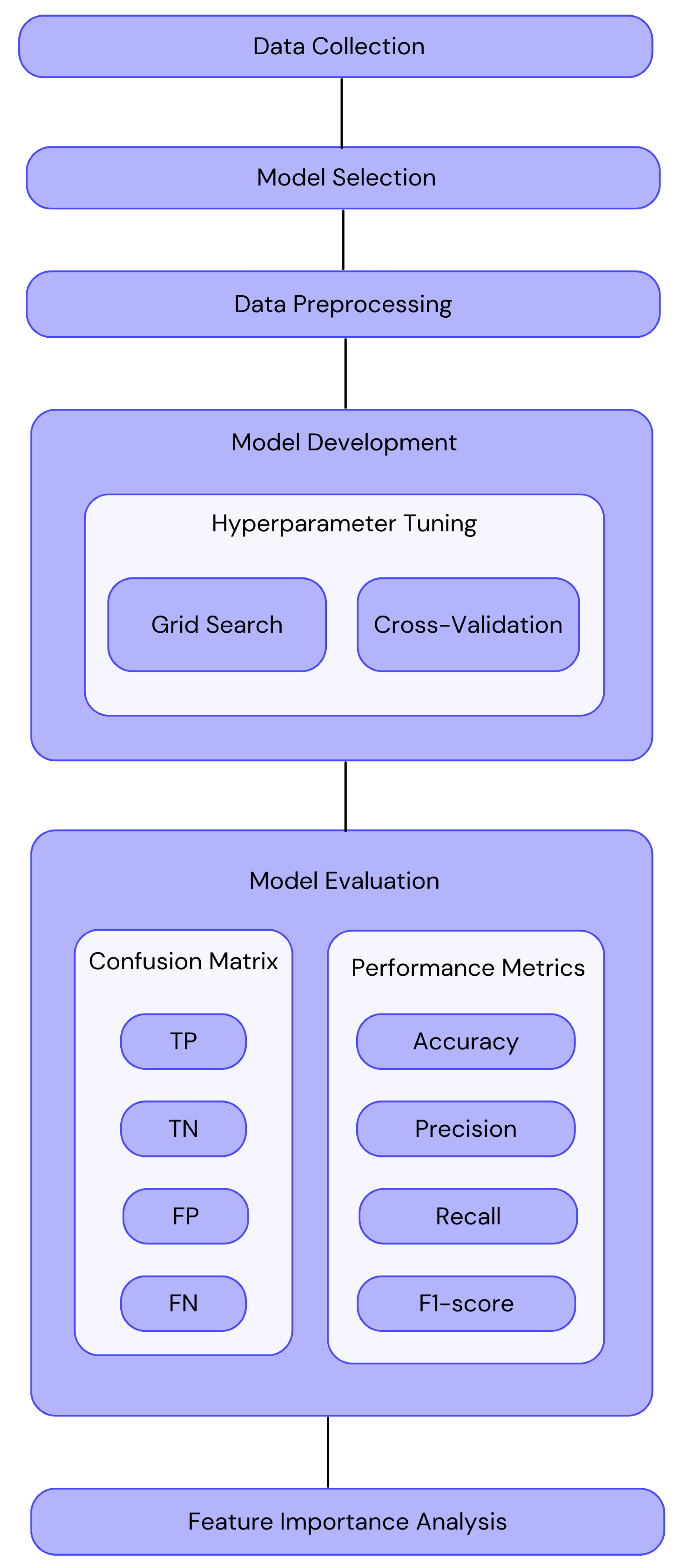
Figure 2.
Evaluation metrics before resampling.
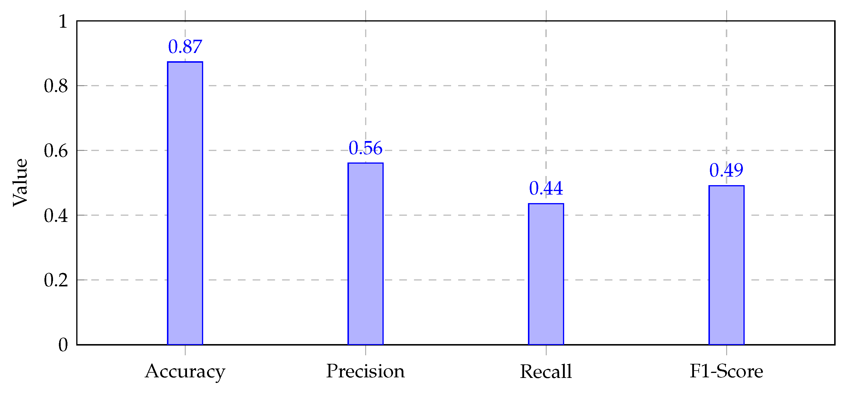
Figure 4.
Feature Importance Scores.
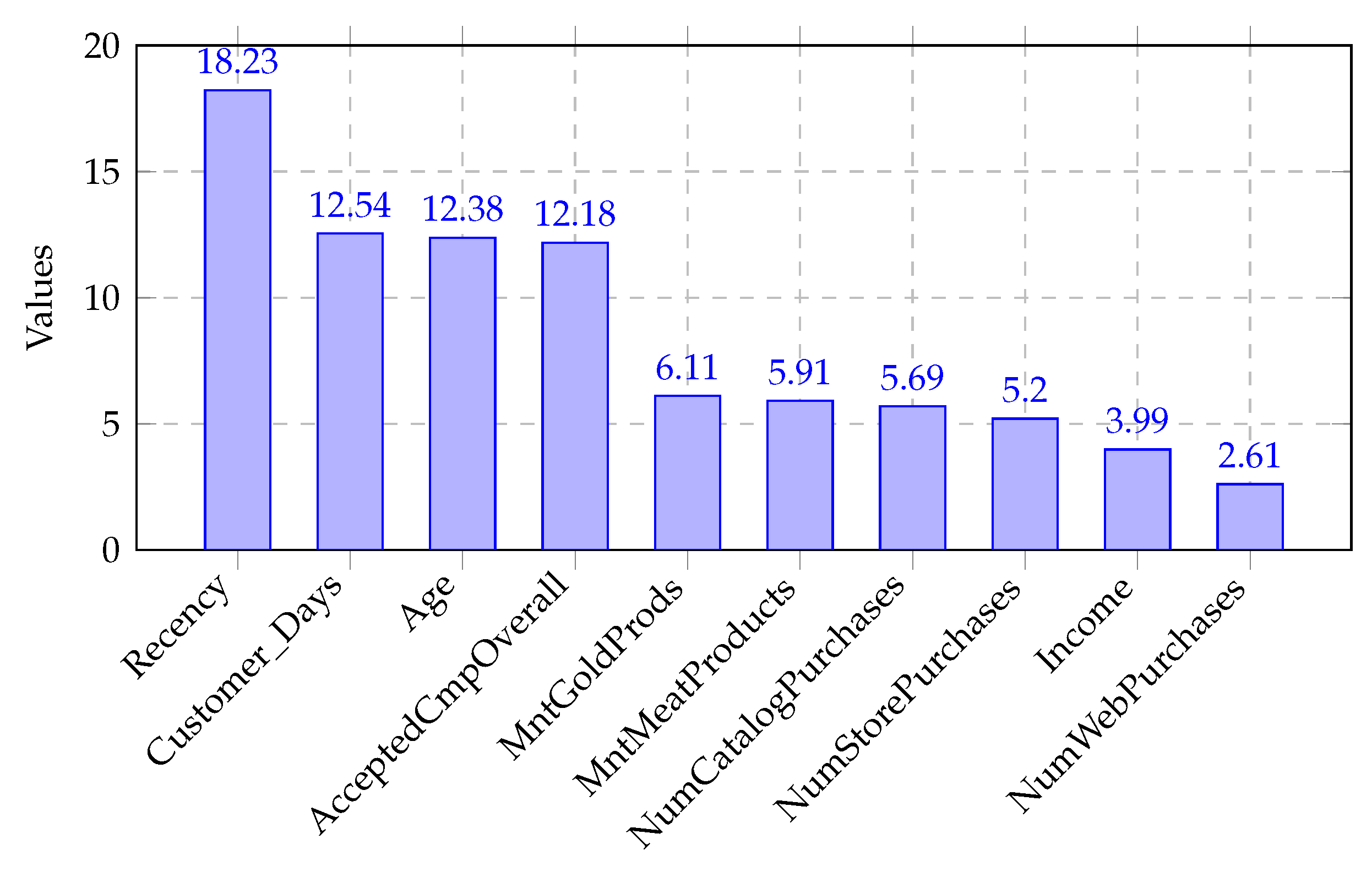
Table 2.
Hardware and Software Configurations.
| Component | Configuration | |
|---|---|---|
| Hardware | Processor | Intel Core i7-10510U |
| RAM | 16 GB | |
| Storage | 952 GB | |
| OS | Windows 11 Pro | |
| Software | Language | Python |
| Libraries | pandas, seaborn, matplotlib, scikit-learn | |
| Environment | Jupyter Notebook |
Table 3.
Data Dictionary.
| Demographic | Income | Kidhome | Age |
| Teenhome | Customer_Days | marital_Together | |
| marital_Single | marital_Divorced | marital_Widow | |
| education_PhD | education_Master | education_Graduation | |
| education_Basic | education_2n Cycle | ||
| Customer Interaction | MntWines | MntFruits | MntGoldProds |
| MntMeatProducts | MntFishProducts | MntSweetProducts | |
| NumStorePurchases | NumCatalogPurchases | NumWebVisitsMonth | |
| NumDealsPurchases | NumWebPurchases | Recency | |
| Z_CostContact | Z_Revenue | MntTotal | |
| MntRegularProds | Complain | Response | |
| AcceptedCmp1 | AcceptedCmp2 | AcceptedCmp3 | |
| AcceptedCmp4 | AcceptedCmp5 | AcceptedCmpOverall |
Table 4.
Confusion Matrix.
| Predicted \Actual | Positive (+) | Negative (-) |
|---|---|---|
| Positive (+) | TP | FP |
| Negative (-) | FN | TN |
Table 5.
Parameter values before resampling.
| Parameter | Value |
|---|---|
| criterion | entropy |
| max_depth | 5 |
| min_samples_leaf | 2 |
| min_samples_split | 2 |
| splitter | random |
Table 6.
Parameter values after resampling.
| Parameter | Value |
| criterion | entropy |
| max_depth | None |
| min_samples_leaf | 2 |
| min_samples_split | 2 |
| splitter | best |
Table 7.
Confusion matrix before resampling.
| Predicted \Actual | Positive (+) | Negative (-) |
| Positive (+) | ||
| Negative (-) |
Table 8.
Confusion matrix after resampling.
| Predicted \Actual | Positive (+) | Negative (-) |
| Positive (+) | ||
| Negative (-) |
Disclaimer/Publisher’s Note: The statements, opinions and data contained in all publications are solely those of the individual author(s) and contributor(s) and not of MDPI and/or the editor(s). MDPI and/or the editor(s) disclaim responsibility for any injury to people or property resulting from any ideas, methods, instructions or products referred to in the content. |
© 2024 by the authors. Licensee MDPI, Basel, Switzerland. This article is an open access article distributed under the terms and conditions of the Creative Commons Attribution (CC BY) license (http://creativecommons.org/licenses/by/4.0/).
Copyright: This open access article is published under a Creative Commons CC BY 4.0 license, which permit the free download, distribution, and reuse, provided that the author and preprint are cited in any reuse.


