
Submitted:
20 August 2024
Posted:
21 August 2024
You are already at the latest version
Abstract
Two-dimensional periodic Stokes flow of viscous incompressible fluid in a rectangular cavity with constant velocities applied to the top and bottom walls is considered. The study of chaotic advection regimes is reduced to the sequential solving of two problems. To solve the first problem, the analytical method of superposition, that allows to obtain any desired accuracy of the velocity field, is used. To solve the second problem, which is associated with obtaining the trajectories of individual fluid particles, numerical calculations of the Cauchy problem were performed. An analysis of the boundary conditions accuracy was performed based on the control of local integration. The advection of the selected volume of fluid in the rectangular cavity under the periodic motion of walls for a finite period time based on piecewise spline cubic interpolation is modelled. The obtained numerical results agree with well-known experimental data.
Keywords:
stokes flow
; chaotic advection
; mixing
; rectangular cavity
; computer modelling
1. Introduction
The mixing problem of laminar fluid flow is important in microtechnology when developing mixing devices in chemical engineering and microbiology. The interest of researchers in this problem arose not only because of the prevalence of the mixing phenomenon in nature, but also due to the use of various mixing technologies in industry and technology (aerodynamics, oceanology, biology, chemistry). Monitoring the conditions of unstable chemical reactions requires the creation of special microchemical processes that maintain the conditions of chemical reactions in a narrow range of physical parameters. They are capable of mixing high molecular weight compounds in a liquid, the molecules of which cannot withstand high stress.
Analysis of various motions allows to conclude that at the initial stage of flow with different geometric scales, convective mixing mechanisms prevail, and the problem of mixing is reduced to analyzing the processes of deformation of the volume of liquid in the selected velocity field. This problem is related to the Lagrangian description of motion in hydrodynamics and is reduced to the analysis of the system of motion of Lagrangian particles in the Eulerian velocity field. Such a problem in the literature has been called the problem of fluid advection.
Liquid advection is associated with the study of the time deformation of selected volumes or regions (in a two-dimensional case) of a liquid that consists of a large number of particles. Despite the fact that such systems have infinitely many degrees of freedom, special attention is paid to the consolidation of individual fluid parts in hydrodynamic flows. Reducing the number of degrees of freedom allows not only to simplify the analysis of the phenomenon, but also to reveal the main properties and patterns in intensive modes of advection.
The study of chaotic mixing regimes arising in some areas of the flow is reduced to the sequential decoupling of two problems. The first task is to determine the velocity field inside a rectangular cavity for a given fluidity at the boundaries. It is necessary to obtain exact solutions, because the second task is associated with finding the trajectory of movement of individual particles of the fluid in the selected area and the deformation of the boundaries of the fluid associated with a dynamically unstable fluid of movement inside the rectangle. To solve the first problem, let’s use the superposition method, which allows to find the asymptotics of unknown coefficients in a number of general solutions, and thereby allows to obtain the desired accuracy.
2. Literature Analisys
In the Lagrangian representation, the problem of advection of a passive marker particle by a prescribed flow defines a dynamical system. For two-dimensional incompressible flow this system is Hamiltonian and has just one degree of freedom. For unsteady flow the system is non-autonomous and one must in general expect to observe chaotic particle motion. These ideas are developed in [1] and subsequently corroborated through the study of a model which provides an idealization of a stirred tank. In the model the fluid is assumed incompressible and inviscid and its motion wholly two-dimensional.
The heat transfer rate from a solid boundary to a highly viscous fluid can be enhanced significantly by a phenomenon which is called chaotic advection or Lagrangian turbulence. Although the flow is laminar and dominated by viscous forces, some fluid particle trajectories are chaotic due either to a suitable boundary displacement protocol or to a change in geometry. As in turbulent flow, the heat transfer rate enhancement between the boundary and the fluid is intimately linked to the mixing of fluid in the system. Chaotic advection in real Stokes flows, i.e., flows governed by viscous forces and that can be constructed experimentally, is reviewed in paper [2].
The Stokes flow inside a two-dimensional rectangular cavity is analyzed in [3] for a highly viscous, incompressible fluid flow, driven by a single rotlet. Specifically, a rigorous solution of the governing two-dimensional biharmonic equation for the stream function is constructed analytically by means of the superposition principle. With this solution, multicellular flow patterns can be described for narrow cavities, in which the number of flow cells is directly related to the value of the aspect ratio.
Two-dimensional chaotic mixing of similar Newtonian fluids in the presence of an advected dissimilar minor phase fluid body with specified size, interfacial tension, and viscosity ratio was numerically investigated in [4]. Interfacial tension was sufficiently high to allow only small deformations in the dissimilar minor phase body. Mixing was confined to a rectangular cavity with periodically driven upper and lower surfaces. Regions of regular motion (i.e., islands) of comparable size to the minor phase body were eventually destroyed or replaced by the minor phase body. Islands persisted for longer times when the initial separation distance between the minor phase body and island was large or when the viscosity ratio was small. When interfacial tension was small enough to deform the minor phase body more readily, islands showed little indication of instability. Results suggest opportunities for improving mixing uniformity in practical processes and disclose how interactions between dissimilar fluids affect mixing.
In [5,6] considered advection of neutrally buoyant discs in two-dimensional chaotic Stokes flow. The goal of the study is to explore a possibility to enhance laminar mixing in batch-flow mixers. Addition of freely moving bodies to periodically driven chaotic flow renders the flowfield nonperiodic [4], i.e., the Lagrangian chaos of the bodies motion induces Eulerian chaos of the flow that makes mixing more intensive. Simulations were performed using a new variant of the immersed boundaries method that allows the direct numerical simulation of fluid–solid flows on a regular rectangular grid without explicit calculation of the forces that the particles exert on the fluid.
The simultaneous effects of flow pulsation and geometrical perturbation on laminar mixing in curved ducts have been numerically studied in [7] by three different metrics: analysis of the secondary flow patterns, Lyapunov exponents and vorticity vector analysis.
In [8] present the paradigm of "designing for chaos" as a general framework for enhancing mixing in microfluidic applications. Designing for chaos is based on a fundamental understanding of the kinematics underlying the mixing process. Computational and experimental analyses demonstrate the effectiveness of the resulting design in generating chaos in the flow.
In paper [9] modified three-dimensional Navier-Stokes system in unbounded domain, which holds the Poincare inequality, is considered. Unique global solvability is proven, for the corresponding semigroup the existence of the global attractor in strong topology of phase space was ascertained, convergence of the obtained attractors to the set of bounded trajectories of the Navier-Stokes 3D-system is shown.
The present a numerical scheme for approximating the incompressible Navier-Stokes equations based on an auxiliary variable associated with the total system energy in [10]. By introducing a dynamic equation for the auxiliary variable and reformulating the Navier-Stokes equations into an equivalent system, the scheme satisfies a discrete energy stability property in terms of a modified energy and it allows for an efficient solution algorithm and implementation.
The purpose of the work is to perform the analysis of the process of advection of the allocated volume of liquid in a rectangular cavity under the action of tangential velocities applied to the upper and lower walls, using the method of piecewise spline interpolation [11]. The use of cubic spline interpolation on smooth contour segments allows to determine the coordinates of additional points on the boundary of the selected volume with high accuracy. The motion of the walls is set by the law, which was considered in the experimental work of Ottino [12].
3. Analytical Determination of the Velocity Field of a Flow of a Viscous Fluid in a Rectangular Cavity
3.1. The Equation of Motion of a Viscous Fluid in the Stokes Approximation
For consideration, let’s take a two-dimensional flow of a viscous incompressible homogeneous fluid which density is equal to . Inside the cavity of dimensions , where the upper and lower boundaries are movable and the side walls are stationary, the flow moves with constant kinematic viscosity . The Cartesian coordinate system introduced is related to the geometric center of the rectangle (Figure 1). The velocity of the top wall is denoted by , and the bottom one is . The problem is to determine the distribution of the velocity field inside the cavity under consideration.
The flow regime is determined by the Reynolds number Re
where U is a characteristic flow rate , L - geometric scale of the flow, . For this case, the inertial and viscous terms are proportional to and , respectively. The Reynolds number [13] shows the ratio of inertial forces to viscosity forces.
The velocity index for the flow under consideration must be chosen in such a way that the Reynolds number . This approximation in the available sources [14] is called the Stokes approximation.
The motion of a viscous incompressible fluid, that has constant physical properties, can be described by the Navier - Stokes equation and the continuity equation
where - velocity vector, - the main vector of volume forces, p - pressure.
The left part of equation (2) can be written as
This particle is called the inertial term, it represents the acceleration of a fluid particle or substantial acceleration. This term corresponds to the force of inertia and shows the rate of formation of the momentum of a fluid element on which external forces act. On the right side, the first term is responsible for the volume forces. The second term is responsible for the pressure, the third for the viscosity force.
For small Reynolds values, flows are characteristic that are formed in small-scale geometric regions, with small scales of velocities and flows with high viscosity. When the Re numbers are small, the flows begin to develop under the action of viscosity forces, prevail, then the inertial properties of the fluid can be neglected. The formation of such flows occurs under the action of an applied pressure gradient, or they are affected by the motion of the boundaries of the Stokes approximation to an instantaneous change in the velocity field throughout the entire flow region.
The Navier-Stokes equations in the case when the inertial components are neglected for an incompressible fluid, when there are no external volume forces and, taking into account all conservative mass pressure forces, is simplified to the form:
together with the continuity equation (3), it is called the Stokes equation.
This equation is linear with respect to the flow velocity field and pressure distribution, and the time component is not included. So the Stokes equations describe a stationary flow of a viscous incompressible fluid, with constant boundary conditions and a stationary pressure gradient.
For the two-dimensional case, the system of Stokes equations can be represented in the form of three differential equations
Let’s differentiate the first and second equations of system (6) with respect to x and y, making the addition operation, get rid of the pressure, replace the first two equations of system (6) with one third-order differential equation
Let’s introduce a vector stream function , by its expression , that connects the distribution of the velocity field of an incompressible flow [14]. In the two-dimensional case, the vector function has only one component , which connects the components of the velocity field in the following form
Substituting (8) into (7) yields a biharmonic equation with respect to the stream function
Taking into account (8), we conclude that the latter equation describes the distribution of the velocity field in the flow that is considered.
3.2. Stokes Flow in a Rectangular Cavity
The two-dimensional Stokes flow of an incompressible viscous fluid can be described as a biharmonic problem. If the movement is too slow, then the inertial forces with a quadratic velocity can be neglected in comparison with the viscous forces, then the stream function can be satisfied with the biharmonic equation
Euler components of the velocity vector in rectangular coordinates are determined by (8).
The flow in a rectangular cavity , arises with the participation of tangential velocities and on the upper and lower walls, while the side walls remain stationary , and therefore, the boundary conditions for equation (12) have the form:
The velocities and can both depend on coordinate x and on time t simultaneously. Periodic functions with a definite period T and its dependence on time are of particular interest. So the stream function is a solution to the quasi-stationary limiting problem will also be periodic with a period T.
Using the linear boundary value problem (12), (13), the representation for the stream function in a rectangular cavity can be presented as a sum of two functions and describing a symmetric and antisymmetric velocity field. The tangential velocities and applied on the upper and lower walls of the cavity excite these fields. In this case, an arbitrary load velocity with even on X functions and can be represented in the form
3.2.1. Construction of a Solution to a Symmetric Problem with Constant Velocities
Using the superposition method, a solution for a symmetric problem with constant velocities can be constructed as a sum of two Fourier series in the complete orthogonal system of functions [15,16,17]
where , .
The first part of the equation in (15) is the solution for the strip , , while the second part is the solution for the strip , . For the first and second series, there is the required number of degrees of functional freedom in order to satisfy the boundary conditions on two opposite boundaries of the rectangle and to satisfy the requirement of completeness of the system of functions on different sides.
The unknown coefficients of the Fourier series , can be calculated by solving the system
where
and — Fourier coefficients of the even function .
Using the boundary conditions: the first equation is satisfied by the boundary condition at , multiplied by and integrated over x from to a, and the second – by fulfilling the boundary condition at for the desired flow function , multiplied by and integrated over y from to b.
At infinity, the asymptotics of the coefficients , takes the form
In the case when the function is continuous together with the first and second derivatives on the interval we have
Let’s obtain the ratio in this form:
When , then with the increase of m the value of does not fall. This condition affects the stability of the numerical solution of an infinite system.
Let’s consider the case when on the interval . According to the formula
the Fourier coefficients for this case take the form . Therefore, the peculiarity of the system (16) will be that the free members will grow. Therefore, it is impossible to use existing data in the study of the asymptotic nature of the behavior of unknowns in systems of this type, because free members are not satisfied with the necessary decreasing condition [18].
In order to be able to use the method of analysis of regular systems, let’s apply new unknowns and [21] according to formulas
where and are some constants. Substituting (23) into (16), let’s obtain one more system for determining the unknown coefficients.
where
Let’s impose a decreasing condition on and . Set the coefficients
In the equations, the condition of decreasing free terms must be satisfied. As a result, let’s obtain the values of the constants and as a result of equating the main terms to zero
Therefore, the infinite system of linear algebraic equations (24) with respect to unknown coefficients and , in general, is satisfied by the regularity conditions [18] and for such a system the asymptotic law of solutions is true
It follows from this condition that there exists a main solution which is bounded and it can be found using the reduction method. The number of unknowns and is finite (M and L), if to add all the terms following the first M and L, then their sum will be equal to zero. Therefore, in order to find the unknown coefficients and it is necessary to solve a finite system of linear equations.
Next, let’s calculate the unknown stream function . Substituting (23) in (15) and obtain the relation
where
In a rectangular cavity, the terms of the equation and are quantities of the order of that, the series in (24) inside the cavity and on the boundary of the region converge uniformly [15,16,18]. There is no need to improve convergence for these series. But on the border, there are diverging rows and .
To transform the expressions and , let’s use the relation
Let’s perform certain transformations to obtain expressions for and , namely
where
Finding the terms slowly coincide, and adding them, let’s obtain the functions and . Now, in expression (24), the series uniformly coincide both at all points of the region and on the boundary. For the function and at the boundary of the region, let’s encountered a singularity, so the calculations were carried out on the basis of the passage to the limit.
Let’s analyze the convergence of the series for the velocity field. Velocity components can be calculated using the formulas given above, as the corresponding derivatives with respect to and from the stream function
Based on formula (28), there are expressions for the velocity component
where and is possible to express from formula (31). The coefficients take the form and and and have the sums of terms with constant coefficients and . Expressions for and are as follows
where
components and are expressed by formulas (30), and .
The series that are included in the solution coincide quickly, so it is possible to select a part to sum to the final values. The accuracy of the fulfillment of the boundary conditions is associated with an infinite number of members of the series, when using the reduced series, there is an error in solving the boundary value problem.
3.2.2. Construction of a Solution to an Antisymmetric Problem with Constant Velocities
Similarly to how let’s found the general solution using the superposition method, let’s find the solution to the boundary value problem [15,16]
where .
When the boundary conditions are satisfied, let’s obtain a system of linear algebraic equations for the unknown Fourier coefficients and and write it in the form
— Fourier coefficients of an even function .
Let’s suppose that in between . The Fourier coefficients in this case will have the form
To neglect the influence of a non-decreasing free term, let’s introduce new variables and
At infinity, the asymptotic of the coefficients and takes the form
In the right part there are
For and , the decrease requirement is performed. For system (39), the law of asymptotic expressions can be applied, since it satisfies the regularity conditions [18].
The solution is sought by a simple reduction method. The number of unknowns and is finite (M and K), if to add all the terms following the first and then their sum is equal to zero. To find the unknown coefficients and it is necessary to solve a finite system of linear equations.
Let’s also take and for the known values. Let’s calculate the stream function
where
Let’s use the ratios
to transform and . Performing mathematical transformations, let’s find an expression for
where
The velocity components, as derivatives with respect to x and y of the stream function, can be represented as
where and are expressed from the following formulas with coefficients and
and and have the sums of all components with constant coefficients and , they can be calculated as derivatives with respect to x and y of the component of the stream function ,
where
where
4. Advection of Fluid
4.1. Advection Equations of a Moving Fluid Particle
Any small, non-inert fluid particle moves with a velocity equal to the flow velocity at the point at which it is located. This means that the equality
and this will be the formal expression of advection. This equation is defining in Lagrangian hydromechanics [14]: the kinematics of the fluid itself is such that each particle of the fluid undergoes passive advection.
The velocity of a particle in the two-dimensional case is, of course, given by the rate of change in its position:
where — coordinates of the radius vector of the particle in the Cartesian coordinate system.
The fluid velocity is specified according to other considerations, including solving some system of partial differential equations, for example, the Euler equations, the Navier-Stokes equations, or the Stokes equations. In other words, the analysis of the motion of individual fluid particles provides that a hydrodynamic problem has been solved, which allows for an arbitrary point at an arbitrary time instant to determine the magnitude of the velocity vector of the flow under consideration
Then condition (49) leads to a system of ordinary differential equations, which are called advection equations [19,20]
In other words, equation (52) describes the motion of a Lagrangian liquid particle in an Eulerian velocity field [14].
From the point of view of the theory of dynamical systems, two ordinary differential equations (52) are more than enough to obtain a non-integral or chaotic dynamical system. The right-hand sides of the equations don’t even need to be very complicated.
In two-dimensional space, to obtain a chaotic motion of a particle, it is necessary that the flow depends on time. Stationary 2D advection is integrated.
From the theoretical point of view, the greatest interest from the point of view of the randomness of the motion of individual fluid particles in hydrodynamic systems are two-dimensional flows, since in this case the velocity is the derivative of the stream function and is expressed through formulas.
If equation (8) is combined with advection equations (52), then they turn into Hamiltonian canonical equations for a system with one degree of freedom
with initial conditions at .
Kinematic equations (53) can be interpreted as a Hamiltonian dynamical system with one degree of freedom, where both play the role of canonical variables and are conjugate coordinates. Any of these coordinates can be taken as a generalized coordinate. Then the second Cartesian coordinate will be the conjugate generalized impulse. The stream function plays the role of the Hamiltonian. The phase space in this problem is configuration space.
The system of differential equations (53) describes the motion of passive non-inertial particles in the two-dimensional case in terms of the stream function, regardless of whether the fluid is viscous or not. And here there is neither contradiction nor paradox, because the Hamiltonian nature of kinematics arises precisely from incompressibility. This does not depend on whether the motion is dynamically dissipative or not. To determine the position of the particles, it is necessary to integrate the equations of motion (53) of each particle within a certain time interval.
4.2. Numerical Modeling of Closed Loop Advection Process
After finding the velocity field in a rectangular cavity, one can begin to study the problem of mixing a viscous fluid with slow motions of the Stokes flow. Below there are examples of calculations obtained on the basis of understanding the analytical velocity field. The periodic motion of the rectangular cavity walls is given by
Let the upper wall move from left to right with velocity during the first half of the period, the lower wall is motionless, and the second half of the period, the lower wall moves from right to left with velocity , and the upper wall is motionless.
In the future, it is convenient to normalize the problem to the height of the cavity and to the period T of motion of the boundaries of the rectangular cavity. Let’s introduce a dimensionless parameter characterizing the movement of each of the movable walls, where — modulus of the maximum wall velocity.
As an example, let’s consider the mixing process in a rectangular cavity with parameters and D corresponding to the data of the Ottino experiment [12].
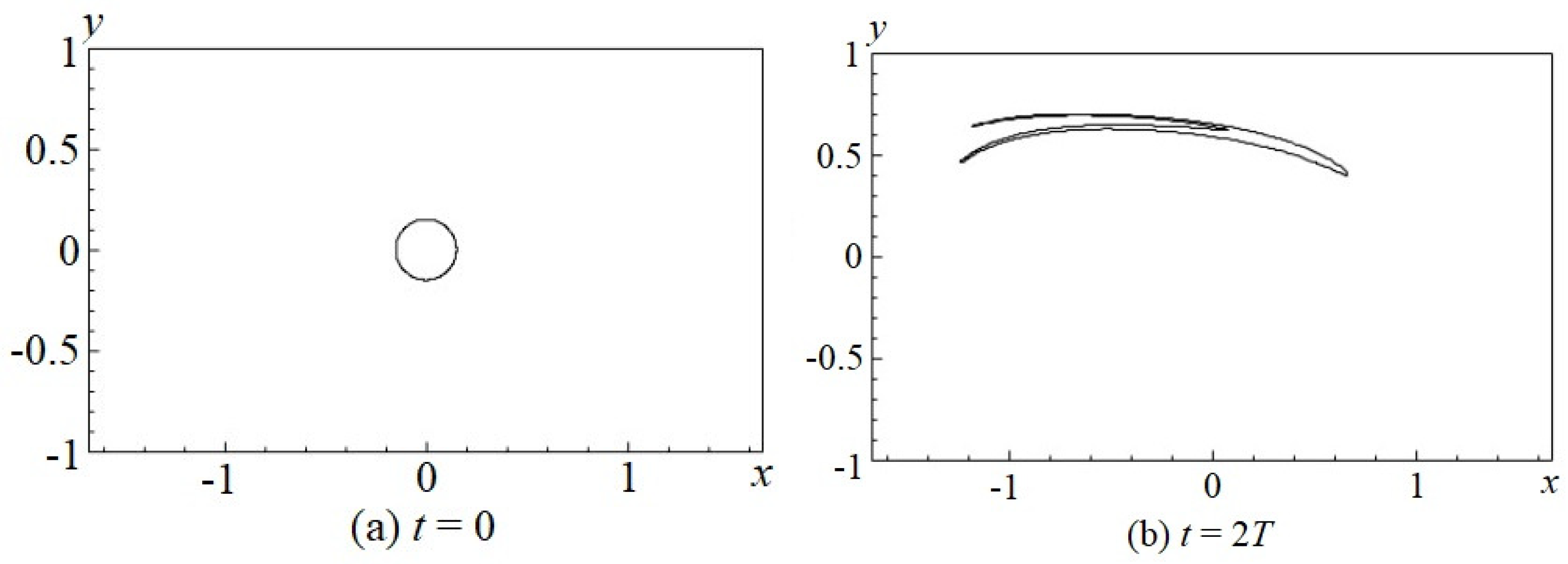
Let’s consider the process of advection of a selected volume of liquid in the form of a circular region of radius centered at the origin, the dimensions of which coincide with the dimensions of the spot from the Ottino experiment. The initial position of the circular spot is shown in Figure 2(a).
In order to numerically simulate the fluid mixing process depicted in Figure 2(f) at , the following procedure was chosen. Let’s fix the value and increase T from 0 to (corresponds to the value ) and monitor the advection process of the selected spot. This approach minimizes the accumulation of error, leads to an erroneous result in the case of a sufficiently large value and consideration of the advection process during only one period T.
It should be noted that the process of advection of the contour is based on piecewise spline cubic interpolation method, developed by Prof. A. Gurzhiy. [11].
The images obtained illustrate that numerical calculations in the process of solving the problem quite accurately illustrate the mixing process. The results are in agreement with the experiment carried out by Ottino [12]. As in the experiment, we obtained the Period-1 island, where the mixing process is not take place (Ottino’s article [12] demonstrates this phenomenon).
5. Conclusions
Using the superposition method, an analytical distribution of the velocity field of the flow of a viscous fluid moving in a rectangular cavity under the action of constant tangential velocities applied to the upper and lower walls is obtained.
The process of mixing the selected volume of fluid with periodic movement of the cavity walls was numerically modeled using the contour advection technique developed by Prof. A. Gurzhiy, and the results obtained are in good agreement with the experimental data.
Author Contributions
Conceptualization, V.S., O.K., O.B., O.P., I.L. and O.V.; methodology, V.S., O.K., O.B., O.P., I.L. and O.V.; formal analysis, V.S., O.K., O.B., O.P., I.L. and O.V.; investigation, V.S., O.K., O.B., O.P., I.L. and O.V.; writing—original draft preparation, V.S., O.K., O.B., O.P., I.L. and O.V.; writing—review and editing, V.S., O.K., O.B., O.P., I.L. and O.V. All authors have read and agreed to the published version of the manuscript.
Funding
The authors express their sincere gratitude for the opportunity to publish the work in this journal on a free basis.
Conflicts of Interest
The authors declare no conflict of interest.
References
- Aref, H. Stirring by chaotic advection. Journal of Fluid Mechanics. 1984, 143, 1–21. [Google Scholar] [CrossRef]
- Lefèvre, A. , Mota, J.P.B., Rodrigo, A.J.S., Saatdjian, E. Chaotic advection and heat transfer enhancement in Stokes flows. International Journal of Heat and Fluid Flow 2003, 24(3), 310–321. [Google Scholar] [CrossRef]
- Van der Woude, D. , Clercx, H.J.H., Van Heijst, G.J.F., Veleshko, V.V. Stokes flow in a rectangular cavity by rotlet forcing. Physics of Fluids 2007, 19(8). [CrossRef]
- Zhang, D. , Zumbrunnen, D.A. Chaotic mixing of two similar fluids in the presence of a third dissimilar fluid. AIChE Journal 1996, 42, 3301–3309. [Google Scholar] [CrossRef]
- Boyland, P.L. , Aref, H., Stremler, M.A. Topological fluid mechanics of stirring. Journal of Fluid Mechanics. 2000, 403, 277–304. [Google Scholar] [CrossRef]
- Vikhansky, A. Chaotic advection of finite-size bodies in a cavity flow. Physic of Fluids 2003, 15(7), 1830–1836. [Google Scholar] [CrossRef]
- Karami, M. , Shirani, E., Jarrahi, H., Peerhossaini, H. Mixing by Time-Dependent Orbits in Spatiotemporal Chaotic Advection. J. Fluids Eng. 2015; 127, 13p, 011201. [Google Scholar] [CrossRef]
- Beebe, D.J., Adrian, R.J., Olsen, M.G., Stremler, M.A., Aref, H., Jo, B.H. Passive mixing in microchannels: Fabrication and flow experiments. Mécanique and Industries. 2001, 2(4), 343–348.
- Gorban, N.V. , Kapustyan, A.V., Kapustyan, E.A., Khomenko, O.V. Strong Global Attractor for the Three-Dimensional Navier-Stokes System of Equations in Unbounded Domain of Channel Type. Journal of Automation and Information Sciences. 2015; 47, 48–59. [Google Scholar] [CrossRef]
- Lianlei Lin, Zhiguo Yang, Suchuan Dong. Numerical approximation of incompressible Navier-Stokes equations based on an auxiliary energy variable. Journal of Computational Physics. 2019, 388, 1–22. [Google Scholar] [CrossRef]
- Gourjii, A.A. , Meleshko, V.V., van Heijst, G.J.F. Method of the Piece-Spline Interpolation in the Advection Problem for an Arbitrary Velocity Field. Dop. AN Ukrainy. 1996, 8, 48–54. [Google Scholar]
- Ottino, J.M. , Leong, C.W. Experiments on mixing due to chaotic advection in a cavity. Journal of Fluid Mechanics 1989, 209, 463–499. [Google Scholar] [CrossRef]
- Meyer, R.E. Introduction to Mathematical Fluid Dynamics; Dover Publications, New York, USA, 2010; 190 p.
- Milne-Thomson, L.M. Theoretical Hydrodynamics; Dover Publications, 5th ed. Edition, New York, USA, 2013; 768 p.
- Meleshko, V.V. Steady Stokes flow in a rectangular cavity. Proceedings of the Royal Society of London 1996, 452(1952), 1999–2022. [Google Scholar] [CrossRef]
- Meleshko, V.V. , Kurylko, O.B., Gourjii, O.A. Generation of topological chaos in the stokes flow in a rectangular cavity. Journal of Mathematical Sciences (United States). 2012, 185(6), 858-871. [CrossRef]
- Sobchuk, V. , Barabash, O., Musienko, A., Tsyganivska, I., Kurylko, O. Mathematical Model of Cyber Risks Management Based on the Expansion of Piecewise Continuous Analytical Approximation Functions of Cyber Attacks in the Fourier Series. Axioms 2023, 12(10), 924. [Google Scholar] [CrossRef]
- Gomilko, A. , Savytskiy O., Trofymchuk O. Superposition, Eigenfunctions and Orthogonal Polynomials Methods in Elasticity and Acoustic Boundary Value Problems. Kyiv: Naukova dumka. 2016, 436. [Google Scholar]
- Aref, H. The development of chaotic advection. Physics of Fluids. 2002, 14(4), 1315–1325. [Google Scholar] [CrossRef]
- Aref, H. Chaotic advection of fluid particles. Philosophical Transactions of the Royal Society of London. 1990, 333(1631). [CrossRef]
- Sobchuk, V. V. , Zelenska, I. O. Construction of asymptotics of the solution for a system of singularly perturbed equations by the method of essentially singular functions. Bulletin of Taras Shevchenko National University of Kyiv. Physics and Mathematics. 2023, 2, 184–192. [Google Scholar] [CrossRef]
Figure 1.
Geometry of a rectangular cavity.
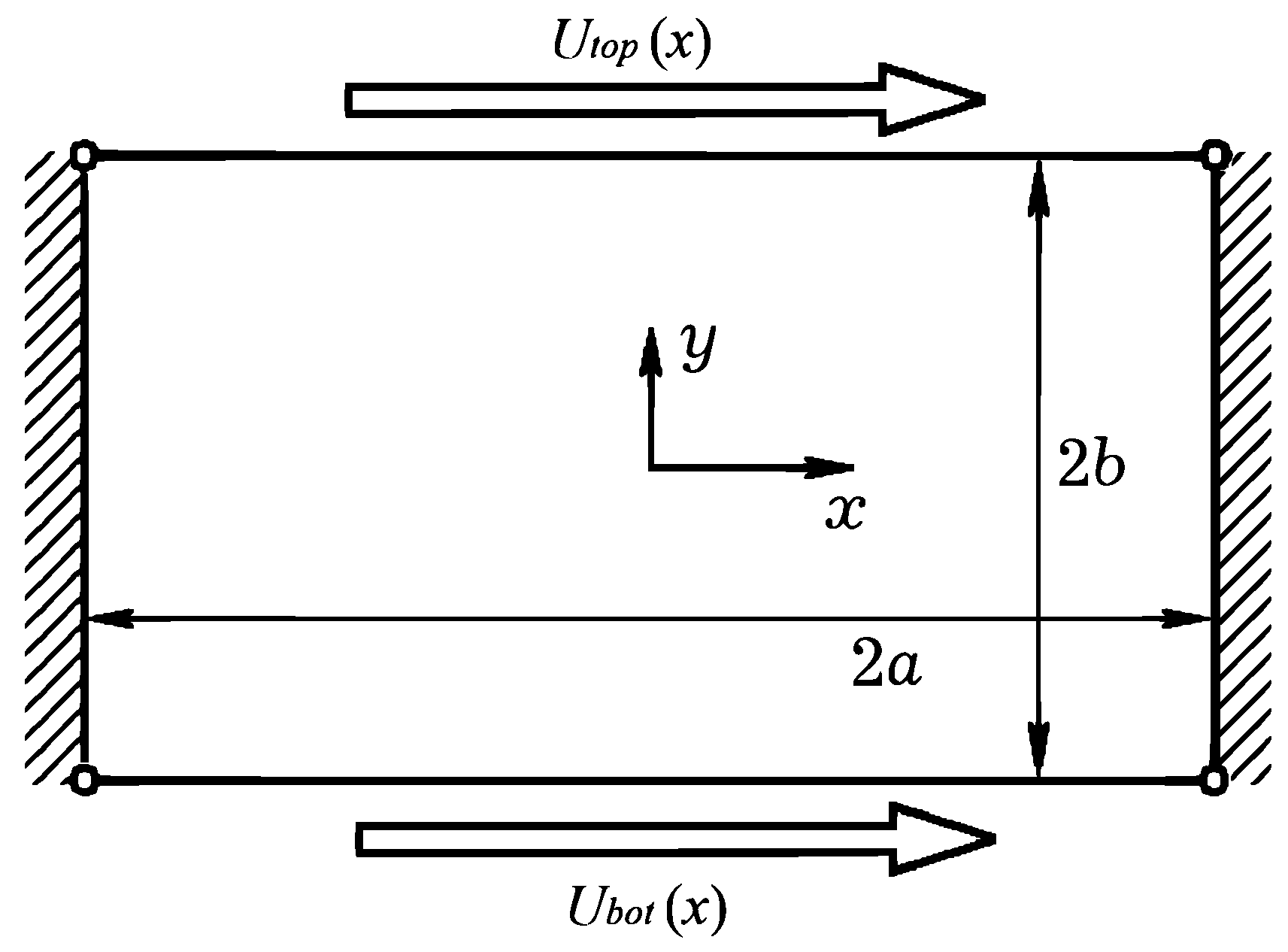
Figure 2.
Deformation of the selected volume of fluid at a constant velocity .

Disclaimer/Publisher’s Note: The statements, opinions and data contained in all publications are solely those of the individual author(s) and contributor(s) and not of MDPI and/or the editor(s). MDPI and/or the editor(s) disclaim responsibility for any injury to people or property resulting from any ideas, methods, instructions or products referred to in the content. |
© 2024 by the authors. Licensee MDPI, Basel, Switzerland. This article is an open access article distributed under the terms and conditions of the Creative Commons Attribution (CC BY) license (http://creativecommons.org/licenses/by/4.0/).
Copyright: This open access article is published under a Creative Commons CC BY 4.0 license, which permit the free download, distribution, and reuse, provided that the author and preprint are cited in any reuse.


