Submitted:
16 August 2024
Posted:
16 August 2024
You are already at the latest version
Abstract
Clustering is a very common analysis of data present in large datasets, with the aims of
understanding and summarizing data, and discovering similarities, among others. However, despite
the present success of subsymbolic methods for data clustering, the description of the obtained
clusters cannot rely on the intricacies of the subsymbolic processing. For clusters of data expressed
in the Resource Description Framework (RDF) we extend and implement an optimized previously
proposed logic-based methodology which computed an RDF structure — called a Common Subsumer
— describing the commonalities among all resources. We tested our implementation with two open,
and very different RDF datasets: one devoted to Public Procurement, and the other devoted to
drugs in Pharmacology. For both datasets, we were able to provide reasonably concise and readable
descriptions of clusters up to 1800 resources. Our analysis shows the viability of our methodology
and computation, and paves the way for general cluster explanations to lay users.
Keywords:
Clusterization
; Explanation in Artificial Intelligence (XAI)
; Least Common Subumer (LCS)
; RDF
1. Introduction and Motivation
Data clusterization is the following problem: given a set of samples (objects, instances, points…) “group samples with similar feature structures or patterns into the same group (cluster) and samples with dissimilar ones into different groups” [1]. Since it can be used without supervision, clusterization is one of the main analysis that can be conducted on big datasets, and it has been successfully applied to collections of nodes in Knowledge Graphs [2], and in the more general setting of RDF graphs, in particular, with the aim to optimize storage and retrieval of RDF resources [3,4,5].
However, depending on the problem, the output of a clusterization algorithm may need to be presented to a human user, either for parameter tuning and debugging, or as a plain result at the end of a workflow [6]. In this situation Clusterization methods too, confront with the general problem of eXplanation in Artificial Intelligence (XAI) [7] and Machine Learning; the problem being that very effective subsymbolic processing lends itself poorly to explanations for lay users, but even for expert users.
With the aim of overcoming such a limitation of subsymbolic clustering of resources in RDF datasets, a post-hoc methodology was previously proposed [8]: once the cluster has been subsymbolically computed,
- exploit the logic substrate which RDF relies on, to compute the most specific RDF graph which is common to all resources in the cluster, known as Least Common Subsumer (LCS) [9]; this phase makes use of blank nodes in RDF, which are existential variables that can abstract — like placeholders, but with a logical semantics — the single values the resources differ on; however, although the LCS is logically complete, it is full of irrelevant details [10];
- compute a Common Subsumer (CS), an RDF structure which is a generalization of the LCS — so, logically, a CS is not the most specific description of the cluster — but still enough specific to capture the relevant features common to all resources;
- use such a structure to generate a phrase in constrained, but plain English, with the original idea of using English pronouns (that, which) to verbalize blank nodes in relative sentences.
This paper adds several enhancement to the methodology above:
- we propose an optimized algorithm for the computation of the CS of a cluster, scaling up to cluster dimensions not attained before;
- we validate this computation through an extensive experimentation with two, very different, real datasets;
- we collect and analyze data about experiments and discuss the computational properties of the implementation: convergence, expected runtime, and possible heuristics.
To prove the effectiveness and generality of our methodology and implementation, we analyzed two open RDF datasets devoted to very different subjects:
Our results prove the soundness and viability of the modified methodology for real datasets. Our implementation provides a human-oriented tool which could be used in Interactive Clusterization, a recent evolution of Clusterization in which the subsymbolic process can be tuned by a human-in-the-loop feedback [11].
With respect to a classification of Semantic Web applications that has been recently proposed by Colucci et al. [12], this application lays at level II for blank nodes dimension ("consider blank nodes with no denotation"), at level I for deductive capabilities ("no capability") and level IV for explanation ("human-readable format").
The paper continues as follows: in the next section, some preliminary knowledge is provided, to make the paper self-contained. Section 3 describes our computation in terms of methodology and analysis. Experimental results about the implementation of computation are given in Section 4, before closing the paper with a final discussion. We moved to Appendix A more details that would make the presentation heavier.
2. Preliminaries
2.1. Background on RDF Syntax and Simple Entailment
Information in RDF datasets is structured in a so-called RDF-graph, in which resources are connected through RDF triples, which we denote in the text with the form 〈〈 s p o 〉〉 (a ubject, a redicate, an bject)[13]3. These terms can be IRIs, XSD-typed literals, and blank nodes, that we discuss below. In the above triple, s is an IRI or a blank node, p is an IRI, and o is either an IRI, or a blank node, or a literal. Triples can be serialized in one of several text-based, machine-readable formats, such as RDF/XML, NTriples, Turtle, etc., so that files/streams of triples can be easily exchanged through HTTP or other text-based Internet protocols. For instance, in Berners-Lee’s Turtle format4, the above triple would be written as
(with a full stop at the end). When most of IRI share the same prefix, the Turtle format allows it to be declared, as in the following example taken from Drugbank:
@prefix ns2: <http://bio2rdf.org/drugbank_vocabulary:> .
@prefix rdf: <http://www.w3.org/1999/02/22-rdf-syntax-ns#> .
ns2:Humans-and-other-mammals rdf:type ns2:Affected-organism .
whose triple (third line) can be read as nearly plain English, but for prefixes that give a machine the Web reference to where such terms are defined (intuitively, a context that defines what they mean).
In addition to being a widely used data interchange format, RDF is also equipped with a formal semantics clearly defined and explained by the W3C [15]. A set of RDF triples is a set of formulas. Triples involving only IRIs and literals correspond to atomic, ground sentences whose First-Order Logic (FOL) notation would be . Following a well-known (non-normative) convention [15], we denote blank nodes by an underscore and a colon, followed by an identifier, e.g., _:x. Blank nodes are existentially quantified variables, whose scope spans through the entire set of triples — usually, a file. Hence, a triple containing a blank node corresponds to an open formula, and if a blank node _:x occurs in several triples of the same file,e.g., if_:x occurs in the two triples
| ex:a ex:r _:x . | and | _:x ex:q ex:b . |
it is considered as the same variable, existentially quantified once, equivalent to the FOL formula 5. Sets of RDF triples are usually called RDF graphs, although they might not be graphs in the ordinary sense, since the following pair of triples is legal:
| ex:a ex:p ex:b . | and | ex:p ex:q ex:d . |
where the subject of the second triple is the predicate of the first one.
An instance of an RDF graph G maps IRIs and literals to themselves, while a blank node is mapped to a term (another blank node, or IRI, or literal).
Thanks to its higher-order semantics (which we do not discuss here), RDF is equipped with a Simple Entailment relation [15], denoted by ⊧ : an RDF graph G entails another RDF graph H, denoted by , if and only if there exists an instance such that , is a subset of G. By Logical equivalence we mean mutual Simple Entailment, i.e., G and H are equivalent if both and hold. Note also the following fact:
Since RDF graphs may expand to billions of triples through Linked Open Data repositories, for each resource r it is common to isolate only a connected portion of an RDF graph centered around the resource [16,17], and compare such structures in order to decide how to group resources. To select the triples that form the relevant properties of r, we apply both a notion of distance, and a filter on stop patterns[18], denoted by a boolean predicate . For example, stop patterns include labels of the resource in all but one chosen language, or the date/authorship of the last edit of a resource properties. We call such portions of an RDF dataset, centered around a root r, a rooted RDF-graph (that we abbreviate as r-graph), denoted by 〈r, Tr〉 Simple Entailment in RDF can be extended to r-graphs, denoted similarly as 〈a, Ta〉 ⊧ 〈b, Tb〉, by carefully mapping roots into roots whenever possible (and otherwise fail) [9].
2.2. Background on Common Subsumers in
To describe the commonalities of the RDF resources, the notion of Least Common Subsumer (LCS) was proposed [9,16], borrowing its name from an analogous notion in Description Logics [19]. The LCS of a set of r-graphs , is a new r-graph 〈x, Tx〉, represented by a new blank node x (one that does not occur in the previous graphs), along with a set of connected triples whose features are all and only the ones shared by all resources — more formally:
- P1:
- for all and
- P2:
- any other r-graph with Property (P1) is logically equivalent to 〈x, Tx〉.
Intuitively, since blank nodes in RDF represent existential variables, it is natural to use a new one of them as an abstraction of several resources — the inverse operation being to instantiate back the blank node with each resource. Moreover, when the resources share only part of the information in a triple, the LCS reports the common information, and abstracts the different characteristics with (another) blank node, say y. We illustrate this intuition below, with an example excerpted from a real dataset.
Consider two drugs Piroxicam and Tolterodine, which are modeled in Drugbank as RDF resources:
- Piroxicam: http://bio2rdf.org/drugbank:DB00554
- Tolterodine: http://bio2rdf.org/drugbank:DB01036
Let us suppose that the RDF graphs TPiroxicam and TTolterodine below (simplified from the original ones to ease readability of the example) are used for computing their LCS. The RDF graphs are serialized in Turtle syntax as follows (we declare common prefixes to ease subsequent reading):
@prefix ns1:<http://bio2rdf.org/drugbank:> .
@prefix ns2: <http://bio2rdf.org/drugbank_vocabulary:> .
@prefix rdf: <http://www.w3.org/1999/02/22-rdf-syntax-ns#> .
TPiroxicam =
- ns1:
-
DB00554 ns2:affected-organism ns2:Humans-and-other-mammals;ns2:category ns2:Anti-Inflammatory-Agents,-Non-Steroidal;ns2:enzyme ns1:BE0002793.
- ns2:
- Humans-and-other-mammals rdf:type ns2:Affected-organism.
- ns2:
- Anti-Inflammatory-Agents,-Non-Steroidal rdf:type ns2:Category.
- ns1:
-
BE0002793 rdf:type ns2:Enzyme;ns2:cellular-location "Endoplasmic reticulum".
TTolterodine =
- ns1:
-
DB01036> ns2:affected-organism ns2:Humans-and-other-mammals;ns2:category ns2:Muscarinic-Antagonists.ns2:enzyme ns1:BE0002793.
- ns2:
- Humans-and-other-mammals rdf:type ns2:Affected-organism.
- ns2:
- Muscarinic-Antagonists rdf:type ns2:Category.
- ns1:
-
BE0002793 rdf:type ns2:Enzyme;ns2:cellular-location "Endoplasmic reticulum".
Then, an RDF graph which is logically implied by both TPiroxicam and TTolterodine is the following:
Tx =
- _:x
-
ns2:affected-organism ns2:Humans-and-other-mammals;ns1:category _:y;ns2:enzyme ns1:BE0002793.
- ns2:
- Humans-and-other-mammals rdf:type ns2:Affected-organism.
- _:y
- rdf:type ns2:Category.
- ns1:
-
BE0002793 rdf:type ns2:Enzyme;ns2:cellular-location "Endoplasmic reticulum".
It was proved [9] that is unique modulo logical equivalence, and that the operation of computing an LCS is idempotent, commutative and associative. However, when used in real contexts [18] the LCS revealed to be too specific and full of details to be useful as the basis for an explanation of commonalities. Moreover, theoretical results [17,20] show that there are sets of resources whose LCS has inherently an exponential size.
Therefore, we reverted to compute a Common Subsumer (CS) of a set of resources, which is more general (less specific) than the least one, but retains enough useful information to be described. Formally, a common subsumer shares with the LCS Property (P1) above, but not Property (P2). Yet, once the method for computing the CS is fixed and uniform, it still enjoys the three properties of being
- CSP1:
- idempotent: ,
- CSP2:
- commutative: and
- CSP3:
- associative:
(we omitted the triples associated to the r-graph for readability) where Properties 2–3 ensure that it can be computed incrementally starting from any “seed pair” of resources, and combining the result with the next resource, and so on iteratively till the last one, since each possible ordering of the resources used in this iteration leads to an RDF graph which is logically equivalent to the one obtained by any other ordering. However, the size of the final (all equivalent) CSs may vary, possibly ranging from the most succinct to a very redundant one — for instance, when several blank nodes are used to represent a structure that could be represented also by a single one. Moreover, also the time needed to compute such a (equivalent form of a) CS may vary a lot.
3. Computation Methodology and Analysis
In this section we present the methodology at the basis of the proposed computation and raise some research questions related to the analysis of such a computation.
The discussion follows the steps below:
- we present an algorithm computing the CS of two resources, which builds on a previously published one, but with a crucial optimization that reduces the size of the resulting CS — still an RDF graph, with blank nodes, but with much less triples than the output of the original algorithm
- exploiting associativity, we iterate the above algorithm computing the CS of a “running” CS (starting with a pair and the next resource , as the expression suggests.
- since the time (and the size) for computing a (equivalent form of) CS of a complete cluster may vary depending on the ordering in which are given, in order to estimate the expected size of a CS of an entire cluster, and the time needed to compute it, we set up a Monte Carlo method, which probes only a random fraction of all the possible orderings, one of which could be used to incrementally compute the CS. We consider the increasing-size heuristic (see Section 3.3 below) as a special trial, and compare its size and time with the other trials
In the above context, we address the following experimental research questions:
- RQ1:
- does the computation of the CS always converges to one size, when changing the order of resources incrementally added to the CS?
- RQ2:
- how quickly converges (depending on the number of resources added to the CS) the incremental computation of a CS of a given cluster?
- RQ3:
- how much the different choices for the next resource to include influence the convergence, and are there simple heuristics that can be used to choose the initial pair, and the next resource?
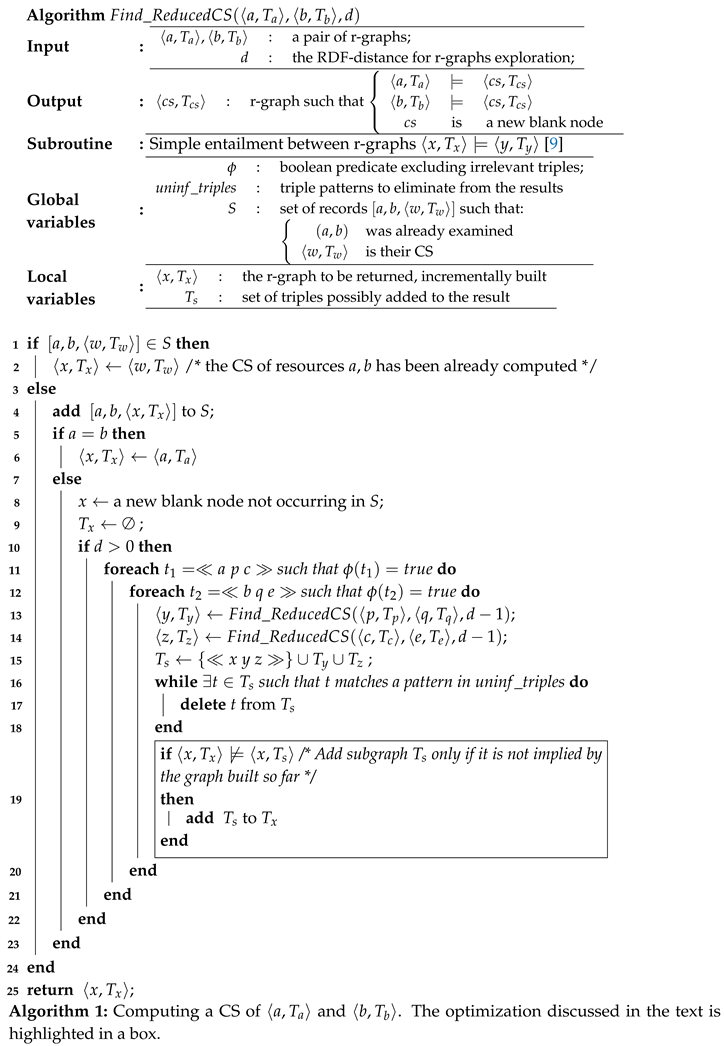
3.1. An Improved Algorithm for the CS of Two Resources (Algorithm 1)
The algorithm performs a joint post-order search in a pair of n-ary trees. It incrementally computes 〈x, Tx〉 by enumerating triples that directly originate from each of the two resources , and recursively calling itself on both the pair of predicates and the pair of objects of these triples. Triples not relevant for the application are filtered away by a predicate . Specifically, for each pair of triples , Algorithm 1 determines with a recursive call a CS 〈y, Ty〉 for the two predicates (Line 13), and a CS 〈z, Tz〉 for the objects (Line 14). It then constructs a provisional r-graph 〈x, Tx〉 with a support variable . Then, the triples in are added to only if 〈x, Tx〉 does not already entail 〈x, Tx〉 (Line 19, boxed for reader’s convenience). The conditional addition overcomes a major drawback of the previously known algorithm, which always added a new subgraph to the result, even when that subgraph was already entailed by the CS being built so far.
Note that Line 19 is merely an optimization step, as it has been demonstrated that the size of the Least Common Subsumer can grow exponentially with the number of resources [17,20] 6.
Regarding time complexity, note that Algorithm 1 could be called with both arguments being the same R-graph 〈x, G〉. It is well known that determining a lean7 equivalent of an RDF-graph G is NP-complete [21]. Since Algorithm 1 operates polynomially in the sizes of its arguments, it is unrealistic to expect it to return a lean (i.e., minimal) r-graph, unless . Nonetheless, in the real RDF datasets we tested, our optimization significantly reduces the CS size.
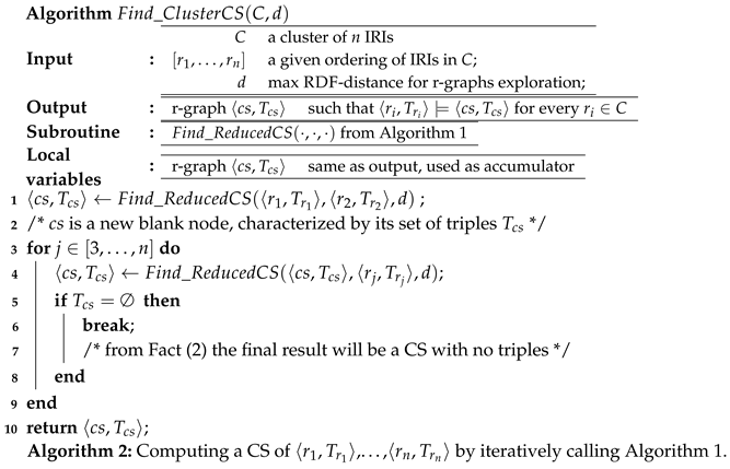
3.2. Computing the CS of a Cluster of Resources (Algorithm 2)
Let be an enumeration of the resources of the cluster in a given order, each resource equipped with the triples describing its relevant characteristics. We can compute the CS of a cluster of resources as that is, by first computing with Algorithm 1 the CS of , then computing the CS of the previous result and Resource , till the CS with the last resource is computed. Associativity and commutativity ensure that any order in which the resources are taken leads to the same result, up to logical equivalence.
3.3. Expected Size of the Final CS, and Overall Runtime of Algorithm 2
With the real datasets we experimented with, the size of a cluster can go up to around 1800 resources. Hence, the incremental computation of the CS of all resources may vary significantly, depending on the order in which the resources are added to the CS, and with Big Data, one cannot even expect to have all resources available at once in order to decide which is the next best one to combine in the CS — resources can arrive as a stream and might need to be collected as they arrive. Hence, we can only estimate the runtime needed and the size of the resulting CS, for the clusters in the datasets we analyzed. We do this with a Monte Carlo method [22], mediating on 100 trials over random orderings of the resources.
When resources are all available at once, an intuitive heuristic is the Increasing-size heuristic: start by computing the CS of the resources r1, r2 whose attached set of triples are the smallest ones, and proceed with resources with an increasing number of triples — after all, few characteristics should mean few commonalities to start with in Line 1, and one may imagine that while examining other resources, only such few established commonalities will be confirmed as the common ones. To confirm or deny such hypothesis, we treat as a special, non-random, case the increasing-size order, and mark it in the experiments to see if its runtime places in the lower part (possibly, the minimum) of the distribution of runtimes, or not. We show in the next section that this intuition fails quite often.
4. Results
Our experiments aim to answer the above research questions by computing the CS of several clusters of RDF resources, obtained by applying the well-known clustering algorithm k-means [23] to the resources in the two datasets TheyBuyForYou and Drugbank mentioned earlier in this paper. For the sake of synthesis, we only discuss here the full experiment with reference to TheyBuyForYou. Details and results about the same experiment in Drugbank may be found in Appendix.
The knowledge graph TheyBuyForYou [24] includes an ontology for procurement data, based on the Open Contracting Data Standard (OCDS) [25] . The OCDS data model is built around the concept of a contracting process, whose main phases are planning, tender, award, contract and implementation. Our experiment starts by clustering the contracting processes emitted on 30 January 2019 (3198 resources) by the k-means algorithm. To this aim, such resources need to undergo a vector embedding process, that exploits the embedding strategies proposed by Ristoski et al. [26] and implemented in the pyRDF2Vec8 library. The optimal number k of clusters to be returned by the k-means algorithm is determined by applying two different optimization methods: the Elbow method [27] and Silhouettes analysis [28] on the feature vector resulting from the embedding. Both of these methods suggest . Thus, 10 different clusters are returned by the k-means algorithms applied on the set of 3198 contracting processes.
For each cluster of resources, we randomly chose an ordering (an ordering of indices), then we started by computing the CS of the first couple of resources (Algorithm 2, Line 1), then computed , i.e., the CS of and the third resource in the ordering, and so on (Algorithm 2, Line 4), until we reach the common subsumer of all resources . We repeated this process one hundred times for each cluster, memorizing for each trial:
- the sequence of Common Subsumers progressively computed
- the sequence of sizes of the CS progressively computed
- the overall runtime of Algorithm 2 in that trial
We discuss how we used each memorized information in a separate subsection (below), and finally compare our research questions of Section 2 with the results obtained.
4.1. Logical Convergence
At the end of each trial, we checked the logical equivalence of the computed r-graph 〈cs, Tcs〉 (rooted at the blank node ) with the one previously obtained with a different ordering. In all cases, we obtained a positive result, that is, all the 100 final r-graphs were logically equivalent, confirming Property CSP3: of Common Subsumers.
4.2. Dependency of the Rate of Convergence on the Order of Added Resources
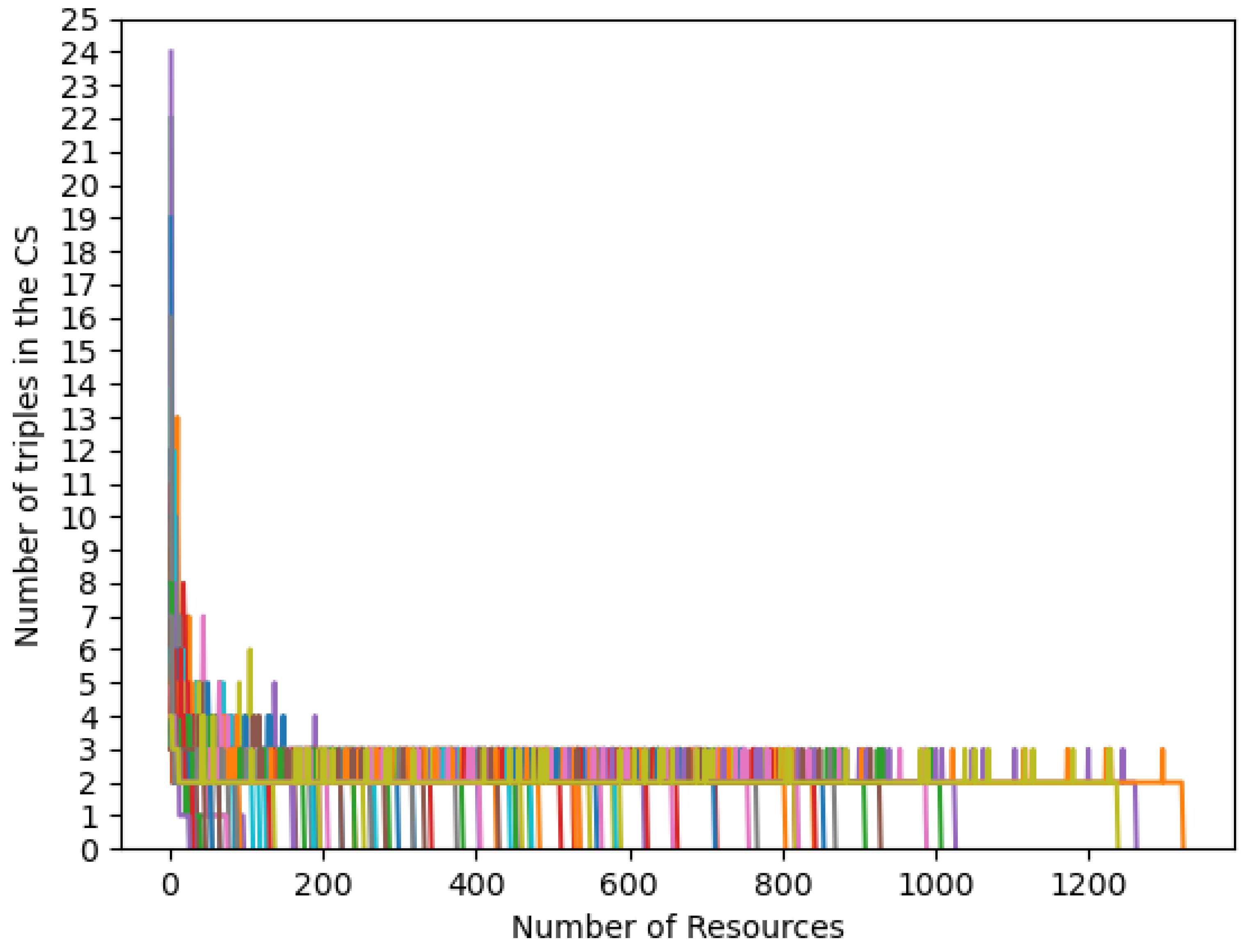
We analyzed the sequence of the sizes of the Common Subsumers, and observed that, while they generally decrease, the rate of such decrement may vary a lot. Figure 1 shows for each cluster how the CS size varies on the number of resources compared in the CS computation. Each chart includes 100 lines that refer to the performed tests, each corresponding to a different random ordering of resources. For the sake of visibility, we show only one of such lines (belonging to Cluster 1) in Figure 2; all other lines have a similar behavior. The reader may notice that the initial size of the CS is 13: The set describing the commonalities of the first two resources includes 13 triples. By adding resources to the computation, the size of CS may decrease, increase, or remain constant. Generally speaking, the final number of triples (6 in the case of Cluster 1) is reached by adding resources (convergence to 6 is reached at 23 resources in the test shown in Figure 2): the larger the collection, the smaller the number of shared features, in most cases. Nevertheless, the CS size may also increase in the number of resources: sometimes the addition of one more resource to the computation causes . In Figure 2 this happens twice: and . This phenomenon highlights a failure in the intuition that the more the resources, the less their commonalities, and hence, also the size of the CS should decrease. For resources expressed in RDF, a commonality can be also that a set of ℓ resources reach the same literal value, say v, through the same path, so that contains that path. If the next resource reaches v too, but through a different path, then might need more blank nodes (and more triples) to represent the different ways in which v is reached.
4.3. Analysis of Computation Time
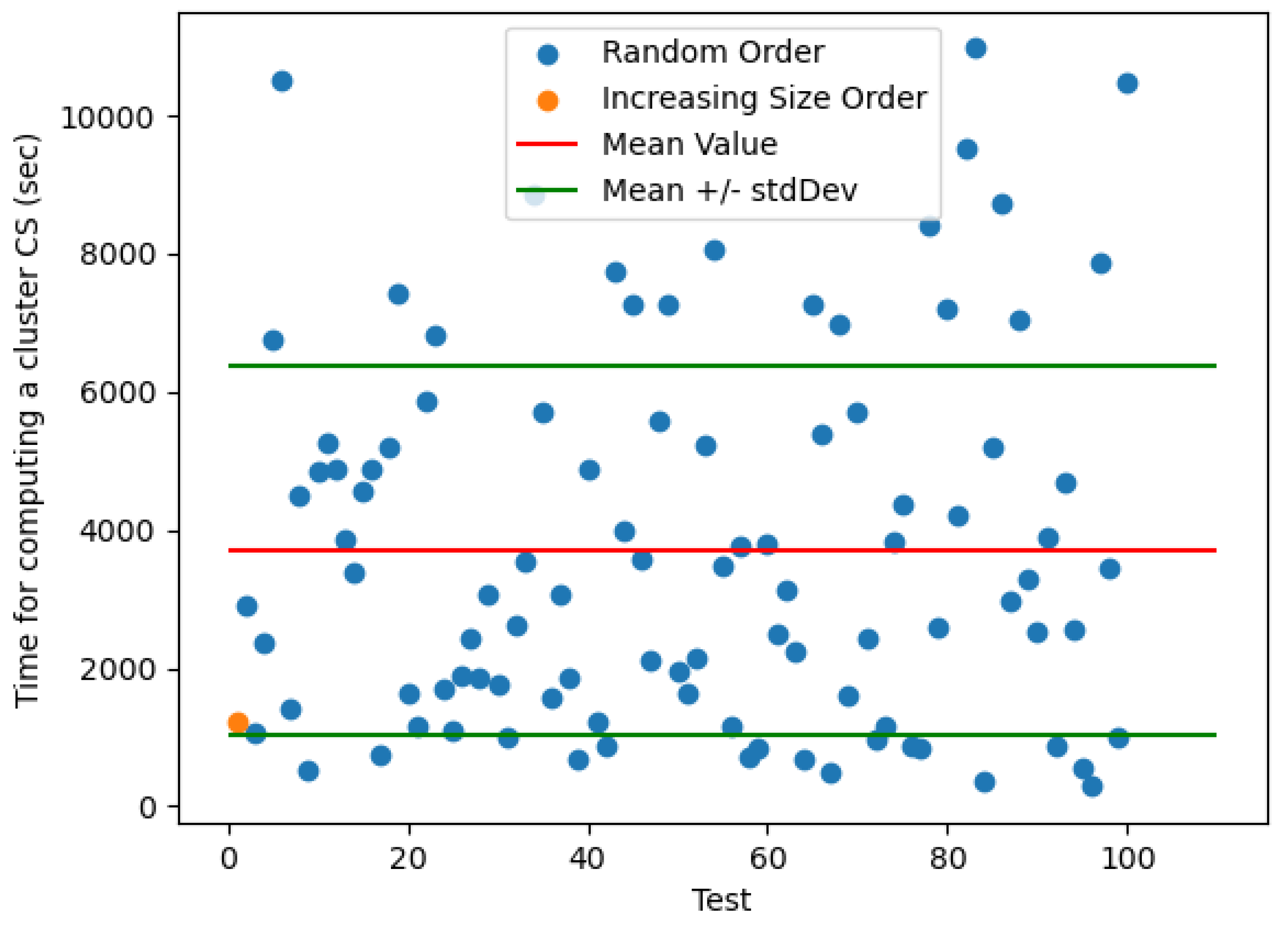
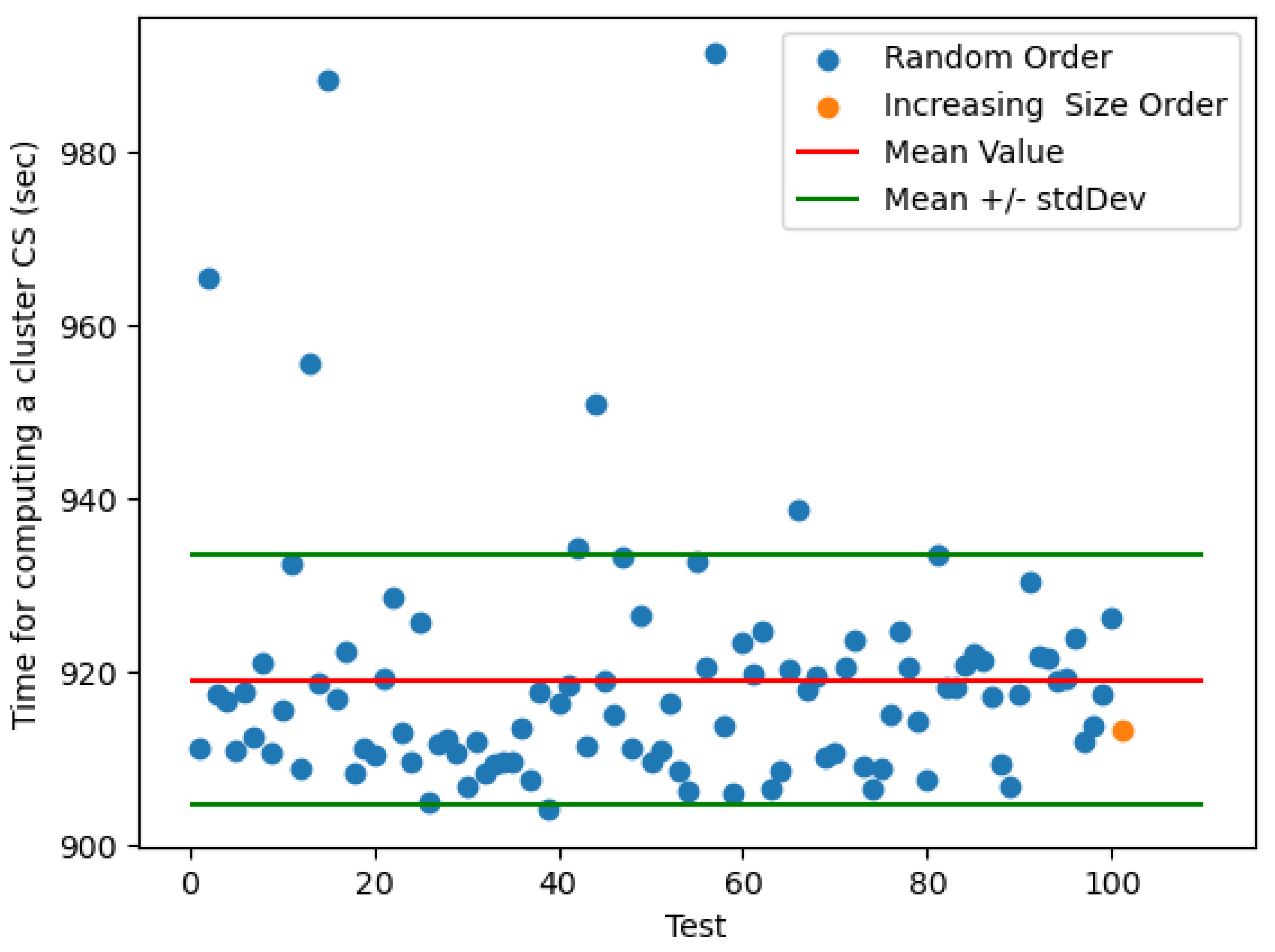
Figure 3 plots in blue the runtime tocompute the CS of Cluster 3 in all the 100 orderings considered in the experiments. We show Cluster 3 as a worst case, because it is the one with the highest mean runtime value (around 935 sec.). We treated as a special case (orange point) the test in which resources are ordered in increasing size. Figure 3 reports also the lines for mean value (red line) plus/minus the standard deviation (green lines), showing that only a small number of tests go outside the range . The distribution is heavy tailed in Statistics terminology, in the sense that most of the outliers (i.e., runtimes outside ) are extremely bigger than .
Surprisingly, the intuition that starting the computation from the resources with the smallest size of , and adding to the CS resources with increasing size, would keep low the number of triples in the running CS and, consequently, the overall execution time, is not true in any of the clusters analyzed: In Cluster 3 (see Figure 3) the orange point is under the mean value for Cluster 3, but it is not the minimal one; in other clusters (not shown), instead, the orange point is close to or even overcomes it (in some cases it corresponds to the maximum computation time). Thus, our experiments did not make evident any heuristic for reducing execution time.
4.4. Final Answers to Research Questions
Given the above results, we can answer the research questions posed in Section 2 (repeated in italic below for convenience) as follows:
- RQ1:
- does the computation of the CS always converges, when changing sequence of resources incrementally added to the CS? — Yes, independently of the sequence in which resources are added to the CS, the CS converges to the same information, represented as logically equivalent, possibly syntactically different, RDF graphs
- RQ2:
- How quickly converges (depending on the number of resources added to the CS) the incremental computation of a CS of a given cluster? — the rate of convergence to a final CS may vary a lot; the experiments reveal that the size of the final CS generally decreases, but not monotonically.
- RQ3:
- how much the different choices for the next resource to include influence the convergence, and are there simple heuristics that can be used to choose the initial pair, and the next resource? — it appears that the heuristic of choosing the resource with the minimum number of triples as the next one does not pay off in real datasets. For two real datasets, we proved that the patterns of the cases that were theoretically proved to be the exponential worst ones, do not show up.
5. Final Discussion
We proposed an optimized algorithm for the computation of a Common Subsumer of clusters of RDF resources. This optimization allows for processing clusters up to about 1800 resources.
The performed experiments show that, independently of the chosen ordering of resources, the computed CS always converges to a final set of triples of the same size, logically equivalent to the CS corresponding to any other ordering. The incremental addition of resources to the computation causes the CS triples set to decrease in size, although not monotonically.
The rate of convergence to the final CS varies a lot on the resource ordering, and the experiments do not reveal any heuristics to make this convergence faster. Future work will investigate on possible heuristics to speed up the CS computation, by choosing the resource ordering.
We also notice that the execution times are much higher in Drugbank than in TheyBuyForYou, despite the emptiness of the CSs of all Drugbank clusters. In other words, the algorithm counter-intuitively takes a longer time to collect less information. By analyzing the resources involved in the computation, we found that drugs do not follow a modeling schema in Drugbank and are modelled according to different patterns. On the contrary, every contracting process in TheyBuyForYou follows the same description schema, that seem to ease the calculus of Common Subsumers.
In our experiments, we computed Common Subsumers of clusters returned by k-means clustering, applied to a numerical representation of RDF resources that exploits vector embedding techniques. By applying state of the art methods (e.g., the elbow method) for determining the optimal number of clusters k, we got a small number (10 in TheyBuyForYou and 6 in Drugbank) of large clusters (up to 400 in TheyBuyForYou and up to 1800 in Drugbank). As a consequence, their CSs are very few-triple sets (even empty sets for Drubgbank): the larger is the cluster, the less is the number of features shared by all cluster items. Such a result suggests different possible corrective solutions. First, one can assume bigger values for the optimal number of clusters k, by denying the optimality of Elbow method as recently proposed by other researchers [29]. Also, the poorness of returned shared information may depend on the loss of information in the embedding process; thus, techniques to make embedding more information-conservative may be investigated. In particular, in an interactive clustering mechanism [30], new walking strategies in the original RDF graph may be proposed, based on the evaluation by end users of the importance of returned commonalities. In other words, users evaluate the human-readable explanation derived by computed CS and this feedback is used to train the walking strategy at the basis of embeddings.
Informed Consent Statement
Not applicable.
Data Availability Statement
The datasets we used in our experiment are publicly available (links checked as of May, 2024): 1. Drugbank: https://download.bio2rdf.org/files/current/drugbank/drugbank.html; 2. TheyBuyForYou: https://tbfy.github.io/data/
Conflicts of Interest
The authors declare no conflicts of interest.
Abbreviations
The following abbreviations are used in this manuscript:
| RDF | Resource Description Framework |
| LCS | Least Common Subsumer |
| CS | Common Subsumer |
Appendix A
We here report some results from the experiments run in the Drugbank dataset [31], useful to paper discussion. DrugBank is a bioinformatics and chemoinformatics resource that combines detailed drug (i.e. chemical, pharmacological and pharmaceutical) data with comprehensive drug target (i.e. sequence, structure, and pathway) information.
In our experiments, we use the RDF representation of Drugbank (https://download.bio2rdf.org/files/current/drugbank/drugbank.html) as datasource. In particular, we apply k-means clustering algorithm to all drugs in Drugbank, after converting the RDF knowledge graph modeling all of them (7670 resources) with pyRDF2Vec embedding libraries. The analysis of optimal k suggests to set . Yet, our experiments reveal that most clusters have an empty CS, and, thus, clusterized resources seem to share no feature. Such a result suggests a re-thinking of embedding process focused on the maintenance of the informative content held by resources and modeled in the original Knowledge graph. Interactive clusterization, suggested as research future direction, may contribute to this focus.
Independently of the quality of clustering results, we use this experiment to check the behaviour of Algorithm 2. In Figure A1, we show the number of triples in the CS of Cluster 1 (1438 resources) in function of the number of resources considered in the computation.
Figure A1.
Drugbank Dataset. Graphical representation of the convergence of the number of triples in the CS with respect to the number of resources considered in the computation (maximum cluster dimension 1438). The chart refers to Cluster 1 and includes 100 lines, one for each tested random permutation of resources. For each line, when the number of triples in the CS decreases to 0, it does not increase anymore (all lines collapse on x axis).
The chart includes 100 lines, all converging to a number of triples in the CS equal to 0. Intuitively, no logical convergence needs to be proved here. Also in this experiment, the convergence rate varies a lot in the 100 tests: some tests get rapidly to the final empty set, while some others analyze almost all resources in the set (see the orange line in Figure A1, converging at resource 1323, as an example).
We also report in Figure A2 the execution times in each of the 100 tests performed in our experiment. The reader may notice that the mean computation time is much higher in Drugbank dataset w.r.t. TheyBuyForYou, despite the emptiness of the returned set of triples. In other words, computing a CS, yet empty, in Drugbank takes much more time than computing a CS populated by some triples in TheyBuyForYou. This is probably due to the lack of a schema for data description in Drugbank, as discussed in paper conclusions.
Figure A2.
Drugbank Dataset. Time for computing the CS of resources in Cluster 1. The orange point plots the computation time for the permutation of resources in increasing size order.
Figure A2.
Drugbank Dataset. Time for computing the CS of resources in Cluster 1. The orange point plots the computation time for the permutation of resources in increasing size order.
References
- Zhou, L.; Du, G.; Lü, K.; Wang, L.; Du, J. A Survey and an Empirical Evaluation of Multi-View Clustering Approaches. ACM Comput. Surv. 2024, 56. [CrossRef]
- Xiao, H.; Chen, Y.; Shi, X. Knowledge Graph Embedding Based on Multi-View Clustering Framework. IEEE Transactions on Knowledge and Data Engineering 2021, 33, 585–596. [CrossRef]
- Bamatraf, S.A.; BinThalab, R.A. Clustering RDF data using K-medoids. 2019 First International Conference of Intelligent Computing and Engineering (ICOICE), 2019, pp. 1–8. [CrossRef]
- Aluç, G.; Özsu, M.T.; Daudjee, K. Building self-clustering RDF databases using Tunable-LSH. VLDB J. 2019, 28, 173–195. [CrossRef]
- Guo, X.; Gao, H.; Zou, Z. WISE: Workload-Aware Partitioning for RDF Systems. Big Data Research 2020, 22. [CrossRef]
- Bandyapadhyay, S.; Fomin, F.V.; Golovach, P.A.; Lochet, W.; Purohit, N.; Simonov, K. How to find a good explanation for clustering? Artif. Intell. 2023, 322.
- Miller, T. Explanation in artificial intelligence: Insights from the social sciences. Artificial Intelligence 2019, 267, 1–38. [CrossRef]
- Colucci, S.; Donini, F.M.; Iurilli, N.; Sciascio, E.D. A Business Intelligence Tool for Explaining Similarity. Model-Driven Organizational and Business Agility - Second International Workshop, MOBA 2022, Leuven, Belgium, June 6-7, 2022, Revised Selected Papers; Babkin, E.; Barjis, J.; Malyzhenkov, P.; Merunka, V., Eds. Springer, 2022, Vol. 457, Lecture Notes in Business Information Processing, pp. 50–64. [CrossRef]
- Colucci, S.; Donini, F.; Giannini, S.; Di Sciascio, E. Defining and computing Least Common Subsumers in RDF. Web Semantics: Science, Services and Agents on the World Wide Web 2016, 39, 62 – 80.
- Colucci, S.; Donini, F.M.; Di Sciascio, E. On the Relevance of Explanation for RDF Resources Similarity. Model-Driven Organizational and Business Agility - Third International Workshop, MOBA 2023. Springer, 2023, Vol. 488, LNBIP, pp. 96–107.
- Bae, J.; Helldin, T.; Riveiro, M.; Nowaczyk, S.; Bouguelia, M.R.; Falkman, G. Interactive clustering: A comprehensive review. ACM Computing Surveys (CSUR) 2020, 53, 1–39.
- Colucci, S.; Donini, F.M.; Di Sciascio, E. A review of reasoning characteristics of RDF-based Semantic Web systems. Wiley Interdisciplinary Reviews: Data Mining and Knowledge Discovery 2024, 14.
- Cyganiak, R.; Wood, D.; Lanthaler, M. RDF 1.1 Concepts and Abstract Syntax, W3C Recommendation, 2014.
- Hartig, O.; Champin, P.A.; Kellogg, G.; Seaborne, A. RDF 1.2 Concepts and Abstract Syntax, W3C Working Draft, 2024.
- Patel-Schneider, P.; Arndt, D.; Haudebourg, T. RDF 1.2 Semantics, W3C Recommendation, 2023.
- Colucci, S.; Donini, F.M.; Di Sciascio, E. Common Subsumbers in RDF. AI*IA-2013. Springer, 2013, Vol. 8249, LNCS, pp. 348–359.
- Amendola, G.; Manna, M.; Ricioppo, A. A logic-based framework for characterizing nexus of similarity within knowledge bases. Information Sciences 2024, 664. [CrossRef]
- Colucci, S.; Donini, F.M.; Sciascio, E.D. Logical comparison over RDF resources in bio-informatics. J. Biomed. Informatics 2017, 76, 87–101. [CrossRef]
- Cohen, W.W.; Borgida, A.; Hirsh, H. Computing Least Common Subsumers in Description Logics. Proceedings of the 10th National Conference on Artificial Intelligence, San Jose, CA, USA, July 12-16, 1992; Swartout, W.R., Ed. AAAI Press / The MIT Press, 1992, pp. 754–760.
- Baader, F.; Küsters, R.; Molitor, R. Computing least common subsumers in description logics with existential restrictions. IJCAI, 1999, Vol. 99, pp. 96–101.
- Pichler, R.; Polleres, A.; Skritek, S.; Woltran, S. Complexity of redundancy detection on RDF graphs in the presence of rules, constraints, and queries. Semantic Web 2013, 4, 351–393.
- Rubinstein, R.Y. Simulation and the Monte Carlo Method, 1st ed.; John Wiley & Sons, Inc.: USA, 1981.
- Jain, A.K.; Dubes, R.C. Algorithms for Clustering Data; Prentice-Hall, Inc.: Upper Saddle River, NJ, USA, 1988.
- Soylu, A.; Corcho, O.; Elvesater, B.; Badenes-Olmedo, C.; Blount, T.; Yedro Martinez, F.; Kovacic, M.; Posinkovic, M.; Makgill, I.; Taggart, C.; Simperl, E.; Lech, T.C.; Roman, D. TheyBuyForYou platform and knowledge graph: Expanding horizons in public procurement with open linked data. Semantic Web 2022, 13.
- Soylu, A.; Elvesæter, B.; Turk, P.; Roman, D.; Corcho, O.; Simperl, E.; Konstantinidis, G.; Lech, T.C. Towards an Ontology for Public Procurement Based on the Open Contracting Data Standard. Proc. of 18th IFIP WG 6.11 Conference on e-Business, e-Services, and e-Society, I3E 2019. Springer-Verlag, 2019.
- Ristoski, P.; Rosati, J.; Noia, T.D.; Leone, R.D.; Paulheim, H. RDF2Vec: RDF graph embeddings and their applications. Semantic Web 2019, 10, 721–752. [CrossRef]
- Marutho, D.; Hendra Handaka, S.; Wijaya, E.; Muljono. The Determination of Cluster Number at k-Mean Using Elbow Method and Purity Evaluation on Headline News. 2018 International Seminar on Application for Technology of Information and Communication, 2018, pp. 533–538. [CrossRef]
- Rousseeuw, P.J. Silhouettes: A graphical aid to the interpretation and validation of cluster analysis. Journal of Computational and Applied Mathematics 1987, 20, 53–65. [CrossRef]
- Schubert, E. Stop using the elbow criterion for k-means and how to choose the number of clusters instead. SIGKDD Explor. Newsl. 2023, 25, 36-42. [CrossRef]
- Bae, J.; Helldin, T.; Riveiro, M.; Nowaczyk, S.; Bouguelia, M.R.; Falkman, G. Interactive Clustering: A Comprehensive Review. ACM Comput. Surv. 2020, 53.
- Wishart, D.S.; Knox, C.; Guo, A.C.; Cheng, D.; Shrivastava, S.; Tzur, D.; Gautam, B.; Hassanali, M. DrugBank: a knowledgebase for drugs, drug actions and drug targets. Nucleic acids research 2008, 36, D901–D906.
| 1 | |
| 2 | |
| 3 | |
| 4 | |
| 5 | Note that this interpretation requires that when RDF files are merged, name conflicts in blank nodes must be standardized apart. This aspect is carefully discussed in the W3C recommendations. |
| 6 | |
| 7 | A lean graph G is an RDF-graph that is ⊆-minimal among all RDF-graphs logically equivalent to G [15]. |
| 8 |
Figure 1.
Each chart refers to one cluster in TheyBuyForYou and includes 100 lines, one for each tested random ordering of resources. In every one of the 100 tests, the number of triples of the CS (vertical axis) converges to a single size as the number of resources added to the CS (horizontal axis) approaches the size of the cluster.
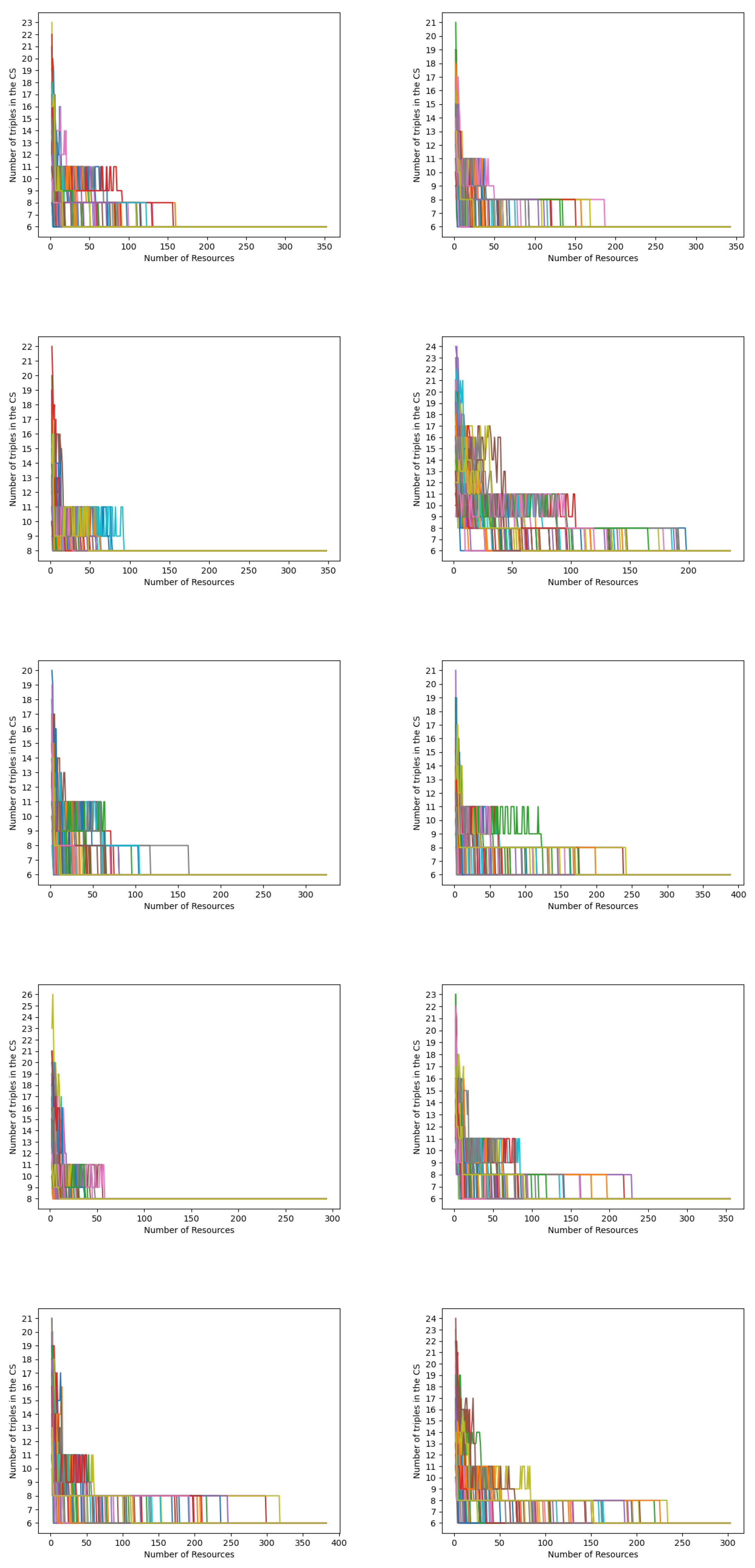
Figure 2.
Convergence of the number of triples in the CS of Cluster 1 with respect to the number of resources considered in the computation. The chart refers to one random ordering of resources.
Figure 2.
Convergence of the number of triples in the CS of Cluster 1 with respect to the number of resources considered in the computation. The chart refers to one random ordering of resources.
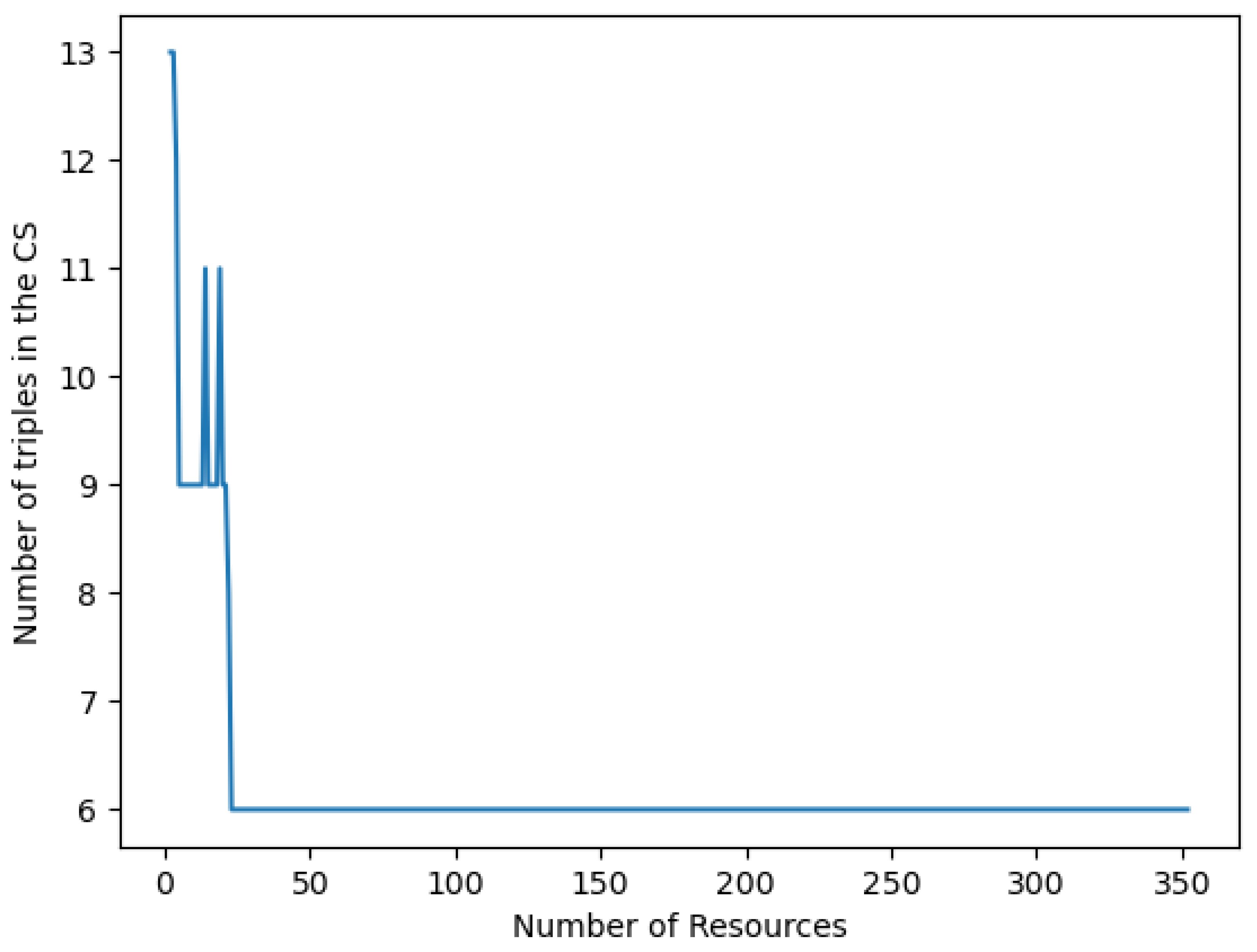
Figure 3.
Time for computing the CS of resources in Cluster 3, the one with the maximum mean value of computation time in 100 different orderings. The orange point plots the computation time for the ordering of resources in increasing size.
Figure 3.
Time for computing the CS of resources in Cluster 3, the one with the maximum mean value of computation time in 100 different orderings. The orange point plots the computation time for the ordering of resources in increasing size.
Disclaimer/Publisher’s Note: The statements, opinions and data contained in all publications are solely those of the individual author(s) and contributor(s) and not of MDPI and/or the editor(s). MDPI and/or the editor(s) disclaim responsibility for any injury to people or property resulting from any ideas, methods, instructions or products referred to in the content. |
© 2024 by the authors. Licensee MDPI, Basel, Switzerland. This article is an open access article distributed under the terms and conditions of the Creative Commons Attribution (CC BY) license (http://creativecommons.org/licenses/by/4.0/).
Copyright: This open access article is published under a Creative Commons CC BY 4.0 license, which permit the free download, distribution, and reuse, provided that the author and preprint are cited in any reuse.


