Submitted:
14 August 2024
Posted:
15 August 2024
You are already at the latest version
Abstract
Assessing the quality of corn seeds necessitates evaluating their content of water, fat, protein, and starch. This study integrates hyperspectral imaging technology with chemometric analysis techniques to achieve non-invasive and rapid detection of multiple key components in corn seeds. Hyperspectral images of the embryo surface of maize seeds were collected within the wavelength range of 1100~2498nm. Subsequently, image segmentation techniques were applied to extract the germ structure of the corn seeds as the region of interest. Seven spectral data preprocessing algorithms were employed, and the Detrending Transformation (DT) algorithm was identified as the optimal preprocessing method through comparative analysis using the Partial Least Squares Regression (PLSR) model. To reduce spectral redundancy and streamline the prediction model, three algorithms were employed for characteristic wavelength extraction: Successive Projections Algorithm (SPA), Competitive Adaptive Reweighted Sampling (CARS), and Uninformative Variable Elimination (UVE). Using both the original spectra and the extracted characteristic wavelengths, four content detection models were constructed: PLSR, Back Propagation Neural Network (BPNN), Radial Basis Function Neural Network (RBFNN), and Least Squares Support Vector Machine (LSSVM). The experimental results demonstrate that the DT-CARS-LSSVM model exhibits exceptional accuracy and stability in predicting these four key components, with determination coefficients of 0.9877, 0.9344, 0.9827, and 0.9592, respectively. This study not only provides a scientific basis for evaluating the quality of corn seeds but also opens up new avenues for the development of non-invasive detection technology in related fields.
Keywords:
Hyperspectral imaging
; Maize
; Content detection
; Non-destructive
; LSSVM
1. Introduction
As the third largest grain crop in the world, maize not only plays a significant role in human diet, but also serves as an important raw material for industrial production. The quality of its seeds is directly related to the yield of corn and the quality of its derivative products. The accurate and efficient detection of component content in corn seeds is of great significance in elevating the overall standards of the corn planting industry and promoting the growth of related industries. Among the various components of corn seeds, the content of water, fat, protein, and starch are key indicators for evaluating seed quality. Water content is an important factor affecting seed storage stability, transportation safety, and germination rate after sowing. High levels of moisture content can accelerate seed respiration, consume nutrients, and even lead to mold and decay; however, too low a water content may cause the seeds to lose vitality and affect germination. Fat, protein, and starch are the main components that constitute the nutritional and economic value of corn seeds, and their content directly determines the nutritional quality and market value of corn. Conventional methods for detecting the composition of corn seeds, such as drying and titration, can meet detection needs to some extent, but they have the disadvantages of being time-consuming, cumbersome to operate, and causing damage to samples, making it difficult to fall short of meeting the needs of rapid, non-destructive, and batch detection in modern agricultural production. Hence, investigating a novel and effective detection technology holds immense importance in enhancing the efficiency and precision of determining the compositional content of corn seeds.
Hyperspectral imaging technology (HSI), an advanced detection method that amalgamates traditional near-infrared spectroscopy with machine vision technology, has gained significant traction in the realm of agricultural product quality assessment in recent years. This technology facilitates swift, non-invasive, and precise analysis of sample composition by capturing spectral data from every pixel on the sample surface and integrating it with spatial information. Over the past few years, it has been subject to extensive research and application in the quality evaluation of agricultural products and food items. [1,2,3,4,5,6]. Liu et al. established a SSA-SVM model based on hyperspectral data to predict the protein content in milk. The prediction results met the accuracy requirements for dairy testing, providing a feasible new method for the rapid detection of milk protein content [7]. Xuan et al. established a multivariate linear regression model for protein content in rice grains based on HSI, with an of 0.9393 in the validation set, providing the possibility for non-destructive protein content detection [8]. Van Haute established a quantitative analysis model between carotene and spectrum based on LSSVM and PLSR, accurately predicting the content of carotene in carrots [9]. Khajehyar et al. used hyperspectral signatures to predict foliar nitrogen and calcium content of tissue cultured little-leaf mockorange (Philadelphus microphyllus A. Gray) shoots, and the values of the established RF regression model reached 0.72 and 0.99 [10]. Zhang et al. combined hyperspectral technology with deep learning algorithms to establish a CNN-LSTM corn seed moisture content detection model, achieving a prediction set R2 of 0.937 [11]. In summary, hyperspectral imaging has shown great potential in predicting the composition content of crops. However, previous studies have primarily focused on detecting individual components, with limited research on simultaneous detection of multiple components, and a lack of in-depth exploration into model optimization. Based on this, this research aims to utilize HSI to quickly and non-destructively detect the moisture, fat, protein, and starch content of corn seeds. By collecting hyperspectral images of corn seeds and combining advanced data processing and analysis methods, a detection model for corn seed composition content based on HSI is established to provide a scientific foundation and technical support for quality control and production management in the corn seed industry.
2. Materials and Methods
2.1. Samples
The samples used in the experiment comprised 80 varieties of corn seeds cultivated in 2023, all from Jilin Province, China. The hulls of these seeds are of similar color, uncoated, and they have plump kernels. Figure 1 shows the photos of some varieties of seeds.
To achieve a stable condition of the seeds and ensure consistency in experimental conditions, prior to the experiment, all seeds were left to stand in the same experimental environment for more than 72 hours, followed by the collection of hyperspectral images. Subsequently, each variety was divided into four aliquots, and their moisture, fat, protein, and starch contents were determined using chemical quantitative methods. Finally, a dataset correlating spectral data with the contents of these components was established.
2.2. Experimental Equipment
The hyperspectral image acquisition equipment used in the experiment mainly including: a 1000–2500 nm imaging spectrometer (ImSpertor N25E); a 1600×1200 pixel CCD camera (Bobcat 1410); a bilateral 150W halogen light source (IT3900); and a one-dimensional precision mobile platform (IRCP-0076-400). During image acquisition, the entire system is placed in a closed dark box to prevent interference from ambient light. The structure of the acquisition system is shown in Figure 2. The spectral acquisition range of the system is 935.5-2539nm, with a resolution of 6.3 nm. In the experiment, through repeated debugging, the lens height was set to 44 cm, the exposure time was set to 10 ms, and the speed of the platform movement was set to 8 mm/s, allowing for the collection of clear images of corn kernels.
Due to the optical properties of the hyperspectral imager’s lens, it generates a large amount of dark current, and the distribution of light intensity also exhibits non-uniformity in certain specific wavelength bands. These factors can result in images obtained from the hyperspectral imager being riddled with a lot of noise. Therefore, to extract useful information from hyperspectral images, it is necessary to perform correction processing on the original image to improve its quality. The image correction formula can be expressed as:
where, R represents the corrected image, Io denotes the original sample image, Iwhite signifies the image captured by scanning the standard whiteboard, and Idark represents a dark field image obtained by covering the camera lens during the experiment
2.3. Method and Principle
2.3.1. Preprocessing Methods
The spectral signal of complex samples is frequently impacted by various factors, including noise, stray light, and baseline shift, with the particle size of the sample being a pivotal factor in spectral measurement [12,13]. Specifically, with the increase in sample particle size, the reproducibility of the spectrum decreases, while the variability of the spectrum increases exponentially. Due to the variations in shape and diameter of individual corn kernels, the resulting spectral data show significant differences, which further complicates the elimination of measurement errors and ultimately impacts the accuracy of quantitative analysis [14]. Therefore, to effectively mitigate spectral noise interference due to factors like seed morphology, it is crucial to employ suitable spectral preprocessing techniques to enhance the quality of spectral data.
To enhance the quality of spectral data and minimize noise and interference, seven preprocessing methods are applied to the spectral data: moving average (MA), Savitzky-Golay derivative convolution (SG), normalization (NOR), baseline correction (BC), multiplicative scatter correction (MSC), standard normal variate transformation (SNV), and detrending transformation (DT). Among them, the window size for MA is 7, and for SG is 7, the polynomial order for SG is 2, and for DT is 2.
2.3.2. Feature Wavelength Extraction Algorithm
1) Successive Projections Algorithms (SPA) Method
SPA is a forward-selection technique that has been traditionally utilized for selecting feature wavelength variables, with the purpose of identifying the combination that reduces redundant information to the greatest extent [15]. The algorithm works by projecting each wavelength onto other bands and comparing the magnitudes of the projection vectors. It selects characteristic wavelengths with minimal redundant information and collinearity, ultimately reducing computation time and enhancing model classification accuracy. SPA selects only a small subset of wavelength variables from the original spectral data, yet these variables capture most of the useful information from the original data. This approach avoids information redundancy, significantly reduces model complexity, and improves the accuracy, speed, and robustness of predictions [16].
2) Uniformative Variable Elimination (UVE) Method
UVE is an algorithm for wavelength selection that utilizes PLSR coefficients. Its primary objective is to refine the modeling dataset by eliminating wavelength variables whose stability is poorer than noise, ultimately improving the predictive power of the model [17]. The method involves combining artificial random noise information with PLS to build a regression cross-validation model. By computing the ratio of the mean to the standard deviation of the regression coefficients, an evaluation metric is established to assess the importance of the characteristic wavelength variables. Furthermore, the maximum value of the noise matrix serves as the upper and lower limits for the algorithm’s threshold, with feature variables exceeding or falling below these thresholds being identified as the final optimized feature vectors.
3) Competitive Adaptive Reweighted Sampling (CARS) Method
The CARS feature extraction algorithm combines Monte Carlo sampling with PLS model regression coefficients [18]. By mimicking Darwin’s “survival of the fittest” principle, it uses adaptive re-weighted sampling (ARS) to progressively discard points with regression coefficients of lower absolute weights, thereby forming a new subset and re-establishing the PLS model. After several iterations, it selects the wavelength subset with the minimum root mean square error of cross-validation (RMSECV) from the PLS model as the characteristic wavelengths. This approach, widely used in spectral data analysis and image processing, effectively reduces data dimensionality and enhances model prediction accuracy.
2.3.3. Modeling Algorithm
1) Partial Least Squares Regression (PLSR)
PLSR, a multivariate data analysis technique in statistics and machine learning, is particularly adept at addressing scenarios involving multicollinearity between dependent and independent variables [19,20]. It merges the strengths of principal component analysis (PCA) and multiple linear regression (MLR), with its central concept revolving around identifying novel orthogonal projection directions, or principal components, that optimize the covariance between the projected dependent and independent variables. This approach facilitates the establishment of a predictive model. Specifically, PLSR introduces latent variables by concurrently analyzing the relationship between the independent variable X and the dependent variable Y, and employs this to construct a linear model between them. Thanks to its unique principles and processes, PLSR is especially proficient in tackling high-dimensional data and small sample regression challenges [21,22].
2) Back Propagation Neural Network (BPNN)
The BPNN, a widely utilized multilayer feedforward neural network in supervised learning tasks, is trained through the error backpropagation algorithm. This model possesses robust nonlinear fitting capabilities, enabling it to automatically learn intricate relationships between input features [23]. A notable advantage of the BPNN model is its capacity to establish a nonlinear model using a limited set of refined wavelength variables. Structurally, it comprises an input layer, a hidden layer, and an output layer [24]. During the network’s learning process, the signal progresses through both forward and backward propagation. Specifically, the input sample is subjected to forward propagation, where it is sequentially processed by the hidden layer, starting from the input layer, and ultimately transmitted to the output layer. In cases where the actual output of the output layer diverges from the desired output, the error undergoes backpropagation. Subsequently, the weights and thresholds of each layer are adjusted along the gradient direction, progressively diminishing the error and ultimately achieving the target accuracy [25].
The number of hidden layer nodes can be determined by an empirical formula, which is calculated as follows:
Where, L and M denote the node counts for the input and output layers, respectively, and α is an integer within the range of 0 to 10.
3) Radial Basis Function Neural Network (RBFNN)
RBFNN is an artificial neural network with a specific architecture, named for the radial basis function (RBF) used as the activation function in the hidden layer [26]. It has found widespread applications in fields such as function approximation, pattern recognition, and control systems. The core idea is to map low-dimensional linearly inseparable data into high-dimensional space, rendering them linearly separable. By carefully selecting the radial basis function and its parameters (such as the center point and width), RBFNN can effectively approximate complex nonlinear functions. As a neural network model, RBFNN possesses strong nonlinear fitting and generalization capabilities. Its unique structure and training algorithm give it significant advantages in dealing with complex nonlinear problems, which is why it has been widely applied in many fields [27,28].
4) Least Squares Support Vector Machine (LSSVM)
LSSVM is an extension of SVM proposed by Suykens et al. It employs the least squares method to find a hyperplane, mapping sample points to a high-dimensional space based on their feature vectors, thus enabling classification or regression predictions for the samples [29]. Compared to traditional SVM, LSSVM replaces the inequality constraints of the slack variable with equality constraints, transforming the problem into solving a system of linear equations, thereby simplifying the calculation process. LSSVM features fast convergence speed, minimal parameter adjustment, strong exploration ability, and high prediction accuracy, making it widely applied in finance, medicine, industry, meteorology, and other fields [30,31].
2.3.4. Model Evaluation Method
The performance of the models was evaluated mainly by the coefficient of determination () and root mean square error (RMSE) [32,33]. The calculation formulas are as follows:
Where, is the actual measured value, is the predicted value, is the average measured value, and represents the average predicted value, is the number of samples. is a value range of [0,1]. The closer is to 1, and the smaller the RMSE is, the better the prediction performance of the regression model.
During the modeling process, if the values of and (determination coefficients of calibration set and validation set) are large with minimal difference, and the values of and (RMSE of calibration set and validation set) are small and the difference is minimal, the model exhibits high reliability and credibility.
3. Results and Discussion
3.1. Sample Division
The samples were partitioned into a calibration set and a prediction set at a 3:1 ratio using the Sample Set Partition Based on Joint X-Y Distance (SPXY) algorithm. Table 1 displays the content statistics of each component in the dataset. The content range of each component within the calibration set encompasses the range present in the prediction set, suggesting that the division of the sample set is appropriate.
3.2. Spectral Extraction and Analysis
The surface structure of a corn kernel comprises the embryo and endosperm, as illustrated in Figure 3. In order to obtain the spectrum of the complete embryo structure region, the seed image is processed using threshold segmentation. Figure 4 shows the spectra of the embryo region, endosperm region, and background region of the corn kernel.
Figure 4 demonstrates that the spectral curve of the embryo exhibits a similarity to the trend observed in the endosperm, yet it shows notable differences when compared to the background spectrum. At 1272.7 nm, 1455.4 nm, and 1871.2 nm, the reflectivity of the embryo and endosperm varies greatly, and the difference in reflectivity between 1272.7 nm and 1871.2 nm is smaller in the embryo structure area than in the endosperm structure area. It is difficult to distinguish the embryo and endosperm regions of some uneven brightness samples by only using the reflection intensity of one band. The band ratio increases the band ratio of the embryo region and decreases the band ratio of the endosperm region. By threshold segmentation, the embryo structure can be effectively segmented from the image. Figure 5 shows the extraction process of the maize kernel embryo.
The wavelength range of hyperspectral data spans from 935.5 nm to 2539 nm, encompassing a total of 256 bands. Due to significant noise interference at the beginning and end of the spectral data during the acquisition process, these segments of data should be excluded from further analysis. Consequently, we utilized 218 bands, ranging from band 22 to band 239 (i.e., the spectrum spanning from 1065 nm to 2432 nm), for our analysis. The average spectral curve of the embryo structure is shown in Figure 6.
Based on the spectral absorption curve, it is observed that the absorption peak located near 1450 nm corresponds to the first-order overtone (or fundamental) vibration of the NH bond present in proteins. Proteins are important components of corn seeds, which are composed of amino acids, and amino acid molecules contain NH bonds. Therefore, when these NH bonds vibrate at the fundamental frequency, an absorption peak near 1450 nm will be generated in the spectrum. The absorption peak near 1950 nm may be related to the carbohydrates in corn seeds, especially the second-order overtone vibration of C-O bonds. Carbohydrates are one of the main components of corn seeds, and they contain a large number of C-O bonds. Therefore, when these C-O bonds vibrate in the second-order overtone mode, corresponding absorption peaks will appear in the spectrum. The absorption peak near 2200 nm involves the combined vibration of OH and NH bonds [34]. In corn seeds, these two bonds are found in molecules such as water and proteins. When they vibrate in specific combinations, they may produce an absorption peak near 2200 nm on the spectrum. These absorption peaks provide us with useful information about the chemical composition and molecular structure of corn seeds. Therefore, it is feasible to quantitatively determine the main component content through the spectral curve of the seeds.
3.3. Spectral Preprocessing
Despite the presence of high multicollinearity among the independent variables, the PLSR model remains applicable for regression modeling. Hence, this study opts for PLSR to assess the effectiveness of different preprocessing methods. The regression model was evaluated using the fit index and the error index RMSE. With the original and preprocessed spectral data as inputs, four component content detection models were established, with the results shown in Table 2. In the table, and represent the determination coefficients for the training and test sets, respectively. The closer the value of is to 1, the better the model’s fit. Generally, a model with an above 0.4 is considered well-fitting. RMSEC and RMSEP respectively denote the root mean square errors of the training and testing sets, and the smaller thet are, the superior the model’s fit.
According to the Table 2, on the whole, the prediction accuracy of the moisture content detection model is higher than that of the other three components. The prediction effect of fat content is relatively poor, with the minimum only having 0.6588. This is primarily because of the low fat content in corn kernels, which involves certain errors in both physical and chemical measurements as well as hyperspectral measurements. The of the four component prediction sets for the original spectra without preprocessing are 0.9748, 0.7483, 0.8995, and 0.8249, respectively, which can better predict the content of each component. For different preprocessing methods, the detection results of different components vary inconsistently. After preprocessing with the MA and SG algorithms, the prediction performance of the model is inferior to that established using the original spectra; NOR improved the prediction effect of protein and starch content, but decreased the prediction effect of moisture and fat content; The BC, MSC, and SNV algorithms have all improved the prediction accuracy for fat, protein, and starch content, but have deteriorated the prediction accuracy for water content; Only when the DT algorithm is applied to preprocess the original spectra, the prediction performance of all components improves, with values being 0.9906, 0.8706, 0.9535, and 0.9145, respectively, and RMSEP values being 0.0393, 0.0606, 0.1057, and 0.2170, respectively. Therefore, in subsequent analysis, DT is selected for spectral preprocessing. The spectral curve after DT preprocessing is shown in Figure 7.
3.4. Feature Wavelength Extraction
Three feature wavelength selection algorithms, SPA, UVE, and CARS, were used to extract the characteristic wavelengths from the preprocessed spectra for various components. The characteristic wavelength positions corresponding to different components are displayed on the average spectral curve, and the extraction results are shown in Figure 8, Figure 9 and Figure 10.
In order to make quantitative predictions for four components simultaneously, the four sets of characteristic wavelengths extracted by each algorithm were combined into a single set. The SPA algorithm extracted a total of 51 characteristic wavelengths, the UVE algorithm extracted a total of 105 characteristic wavelengths, and the CARS algorithm extracted a total of 89 characteristic wavelengths. Table 3 presents the coefficients of determination for the prediction sets of the four components.
3.5. Establishment of a Model for Detecting the Content of Multiple Components in Maize Seeds
The original spectra were preprocessed using the DT algorithm, followed by the extraction of characteristic wavelengths from the preprocessed spectral data. Subsequently, multi-output content detection models were established for PLSR, RBFNN, BPNN, and LSSVM, each based on both full-band spectra and characteristic wavelengths. The prediction performance of these models was evaluated using the coefficient of determination for the prediction set of each component. The results of the model predictions are presented in Table 4, while the prediction effects are illustrated in Figure 11, Figure 12, Figure 13 and Figure 14.
According to the model prediction results, it can be seen that the detection effect of water content in several components is the best, followed by starch content, and the prediction effect of fat content is relatively the worst. Using full-band spectra for modeling, the model prediction performance is better because the spectral data contains information about all seed components. Among the models established based on the full-band spectra, the PLSR model has the best prediction performance, with values of 0.9874, 0.9472, 0.9833, and 0.9532 for moisture, fat, protein, and starch content, respectively. Although the detection of fat content is not as good as that of the full-band RBFNN model, the detection of the other three components is higher than the RBFNN model.
Using feature selection modeling can significantly improve prediction accuracy and modeling efficiency, enhance model stability, and facilitate online real-time monitoring. However, it also has some disadvantages such as a complex algorithm selection process, potential loss of useful information, sensitivity to initial conditions, and potentially high computational demands. Based on the prediction models of PLSR and RBFNN, from the perspective of prediction accuracy, the modeling performance of feature selection is not as good as that of full-spectrum modeling, indicating that during the feature selection process, some wavelengths with weak correlation to the target substance but containing useful information may be removed, resulting in a greater loss of spectral information related to the substance being tested. On the contrary, the BP neural network and LSSVM models have better prediction performance than the full-spectrum model when using feature selection for modeling. The best performance is achieved by the CARS-LSSVM model, with the values of the four components all improving compared to full-spectrum modeling, indicating that these two models can achieve more precise results with less sensitive information. It is not difficult to find that the prediction performance of the LSSVM model is relatively stable across several different input wavelengths, and the detection performance of the four components is relatively good. Based on the comprehensive comparison results, the optimal model for detecting the composition content of corn seeds was determined to be CARS-LSSVM.
4. Conclusions
This study employs HSI to achieve rapid and non-destructive precise detection of multiple key components in corn seeds, including water, fat, protein, and starch. Initially, the embryo structure of the corn seeds was precisely extracted as the region of interest using hyperspectral image segmentation technology. Subsequently, seven spectral data preprocessing algorithms were applied, and DT was identified as the optimal preprocessing method through a comprehensive comparison with the PLSR model. To further our research, we employed three characteristic wavelength extraction strategies: SPA, CARS, and UVE, with the aim of precisely capturing the spectral characteristics of each component. Finally, multi-component content detection models based on raw spectra and characteristic wavelengths were constructed using PLSR, BPNN, RBFNN, and LSSVM, respectively, to achieve comprehensive and in-depth quality assessment of corn seeds. The experimental results demonstrated that the DT-CARS-LSSVM model exhibited outstanding accuracy and stability in predicting the four key components, with coefficients of determination reaching 0.9877, 0.9344, 0.9827, and 0.9592, respectively, highlighting the significant advantages and application potential of this method in the field of corn seed main component content and quality detection. This study not only provides a scientific basis for the quality assessment of corn seeds but also opens up a new path for the development of non-destructive testing technology in related fields.
Author Contributions
Conceptualization, H.X.; Data curation, H.X.; Formal analysis, Y.Y.; Funding acquisition, X.M.; Investigation, H.X.; Methodology, H.X.; Project administration, X.M.; Resources, X.X.; Software, H.X.; Supervision, X.M ; Validation, Y.Y.; Writing—original draft, H.X.; Writing—review & editing, X.X. All authors have read and agreed to the published version of the manuscript.
Funding
This research was funded by Jilin Provincial Department of Science and Technology Development Plan Projec (Grant No. 20220203112S) and Jilin Provincial Department of Education Science and Technology Research Project (Grant No. JJKH20210039KJ).
Institutional Review Board Statement
Not applicable.
Informed Consent Statement
Not applicable.
Data Availability Statement
All relevant data presented in the article are stored according to institutional requirements and, as such, are not available online. However, all data used in this manuscript can be made available upon request to the authors.
Conflicts of Interest
The authors declare no conflict of interest.
References
- Wang, S.N.; Tan, Y.; Liu, C.Y.; Song, S.Z.; Li, Z. Classification and Identification of Soybean Varieties by Density Functional Theory Combined with Raman Spectroscopy. Journal of Sensor Technology and Application 2022, 10, 177–186. [Google Scholar]
- Ruett, M.; Junker-Frohn, L.V.; Siegmann, B.; Ellenberger, J.; Jaenicke, H.; Whitney, C.; Luedeling, E.; Tiede-Arlt, P.; Rascher, U. Hyperspectral Imaging for High-throughput Vitality Monitoring in Ornamental Plant Production. Scientia Horticulturae 2022, 291. [Google Scholar] [CrossRef]
- Muruganantham, P.; Samrat, N.H.; Islam, N.; Johnson, J.; Wibowo, S.; Grandhi, S. Rapid Estimation of Moisture Content in Unpeeled Potato Tubers Using Hyperspectral Imaging. Applied Sciences-Basel 2023, 13. [Google Scholar] [CrossRef]
- Zhang, L.; Zhang, Q.; Wu, J.; Liu, Y.; Yu, L.; Chen, Y. Moisture Detection of Single Corn Seed Based on Hyperspectral Imaging and Deep Learning. Infrared Physics & Technology 2022, 125. [Google Scholar] [CrossRef]
- Wei, X.; Huang, L.; Li, S.; Gao, S.; Jie, D.; Guo, Z.; Zheng, B. Fast Determination of Amylose Content in Lotus Seeds Based on Hyperspectral Imaging. Agronomy-Basel 2023, 13. [Google Scholar] [CrossRef]
- Raj, R.; Cosgun, A.; Kulic, D. Strawberry Water Content Estimation and Ripeness Classification Using Hyperspectral Sensing. Agronomy-Basel 2022, 12. [Google Scholar] [CrossRef]
- Liu, M.; Xue, H.; Liu, J.; Dai, R.; Hu, P.; Huang, Q.; Jiang, X. Hyperspectral Analysis of Milk Protein Content Using SVM Optimized by Sparrow Search Algorithm. Spectroscopy and Spectral Analysis 2022, 42, 1601–1606. [Google Scholar]
- Xuan, G.; Jia, H.; Shao, Y.; Shi, C. Protein Content Prediction of Rice Grains Based on Hyperspectral Imaging. Spectrochimica Acta Part a-Molecular and Biomolecular Spectroscopy 2024, 320. [Google Scholar] [CrossRef] [PubMed]
- Van Haute, S.; Nikkhah, A.; Malavi, D.; Kiani, S. Quantitative Measurement of Internal Quality of Carrots Using Hyperspectral Imaging and Multivariate Analysis. Scientific Reports 2023, 13. [Google Scholar] [CrossRef]
- Khajehyar, R.; Vahidi, M.; Tripepi, R. Using Hyperspectral Signatures for Predicting Foliar Nitrogen and Calcium Content of Tissue Cultured Little-leaf Mockorange (Philadelphus Microphyllus A. Gray) Shoots. Plant Cell Tissue and Organ Culture 2024, 157. [Google Scholar] [CrossRef]
- Zhang, L.; Zhang, Q.; Wu, J.; Liu, Y.; Yu, L.; Chen, Y. Moisture Detection of Single Corn Seed Based on Hyperspectral Imaging and Deep Learning. Infrared Physics & Technology 2022, 125. [Google Scholar] [CrossRef]
- Yu, Z.H.; Chen, X.C.; Zhang, J.C.; Su, Q.; Wang, K.; Liu, W.H. Rapid and Non-destructive Estimation of Moisture Content in Caragana Korshinskii Pellet Feed using Hyperspectral Imaging. Sensors 2023, 23, 7592. [Google Scholar] [CrossRef] [PubMed]
- Yang, W.; Xiong, Y.; Xu, Z.; Li, L.; Du, Y. Piecewise Preprocessing of Near-infrared Spectra for Improving Prediction Ability of a PLS Model. Infrared Physics & Technology 2022, 126. [Google Scholar] [CrossRef]
- Tian, Y.; Sun, L.; Bai, H.; Lu, X.; Fu, Z.; Lv, G.; Zhang, L.; Li, S. Quantitative Detection of Crude Protein in Brown Rice by Near-Infrared Spectroscopy Based on Hybrid Feature Selection. Chemometrics and Intelligent Laboratory Systems 2024, 247. [Google Scholar] [CrossRef]
- Qiao, M.; Xia, G.; Xu, Y.; Cui, T.; Fan, C.; Li, Y.; Han, S.; Qian, J. Generic Prediction Model of Moisture Content for Maize Kernels by Combing Spectral and Color Data through Hyperspectral Imaging. Vibrational Spectroscopy 2024, 131. [Google Scholar] [CrossRef]
- Zhang, F.; Wang, M.; Zhang, F.; Xiong, Y.; Wang, X.; Ali, S.; Zhang, Y.; Fu, S. Hyperspectral Imaging Combined with GA-SVM for Maize Variety Identification. Food Science & Nutrition 2024, 12, 3177–3187. [Google Scholar] [CrossRef]
- Wang, Z.; Chen, J.; Zhang, J.; Tan, X.; Raza, M.A.; Ma, J.; Zhu, Y.; Yang, F.; Yang, W. Assessing Canopy Nitrogen and Carbon Content in Maize by Canopy Spectral Reflectance and Uninformative Variable Elimination. Crop Journal 2022, 10, 1224–1238. [Google Scholar] [CrossRef]
- Sudu, B.; Rong, G.; Guga, S.; Li, K.; Zhi, F.; Guo, Y.; Zhang, J.; Bao, Y. Retrieving SPAD Values of Summer Maize Using UAV Hyperspectral Data Based on Multiple Machine Learning Algorithm. Remote Sensing 2022, 14. [Google Scholar] [CrossRef]
- Ai, N.; Jiang, Y.; Omar, S.; Wang, J.; Xia, L.; Ren, J. Rapid Measurement of Cellulose, Hemicellulose, and Lignin Content in Sargassum horneri by Near-Infrared Spectroscopy and Characteristic Variables Selection Methods. Molecules 2022, 27. [Google Scholar] [CrossRef]
- Lesnoff, M.; Andueza, D.; Barotin, C.; Barre, P.; Bonnal, L.; Pierna, J.A.F.; Picard, F.; Vermeulen, P.; Roger, J.-M. Averaging and Stacking Partial Least Squares Regression Models to Predict the Chemical Compositions and the Nutritive Values of Forages from Spectral Near Infrared Data. Applied Sciences-Basel 2022, 12. [Google Scholar] [CrossRef]
- Rahmawati, L.; Zahra, A.M.; Listanti, R.; Masithoh, R.E.; Hariadi, H. ; Adnan; Syafutri, M.I.; Lidiasari, E.; Amdani, R.Z.; Puspitahati; et al. Necessity of Log(1/R) and Kubelka-Munk Transformation in Chemometrics Analysis to Predict White Rice Flour Adulteration in Brown Rice Flour Using Visible-Near-Infrared Spectroscopy. Food Science and Technology 2023, 43, e116422-e116422. [Google Scholar] [CrossRef]
- Wen, Y.; Li, Z.; Ning, Y.; Yan, Y.; Li, Z.; Wang, N.; Wang, H. Portable Raman Spectroscopy Coupled with PLSR Analysis for Monitoring and Predicting of the Quality of Fresh-Cut Chinese Yam at Different Storage Temperatures. Spectrochimica Acta Part a-Molecular and Biomolecular Spectroscopy 2024, 310. [Google Scholar] [CrossRef] [PubMed]
- Wang, D.; Ni, J.; Du, T. An Image Recognition Method for Coal Gangue Based on ASGS-CWOA and BP Neural Network. Symmetry-Basel 2022, 14. [Google Scholar] [CrossRef]
- Yang, X.; Ni, H.; Li, J.; Lv, J.; Mu, H.; Qi, D. Leaf Recognition Using BP-RBF Hybrid Neural Network. Journal of Forestry Research 2022, 33, 579–589. [Google Scholar] [CrossRef]
- Zhao, J.; Yan, H.; Huang, L. A Joint Method of Spatial-Spectral Features and BP Neural Network for Hyperspectral Image Classification. Egyptian Journal of Remote Sensing and Space Sciences 2023, 26, 107–115. [Google Scholar] [CrossRef]
- Zheng, S.; Feng, R. A Variable Projection Method for the General Radial Basis Function Neural Network. Applied Mathematics and Computation 2023, 451. [Google Scholar] [CrossRef]
- Cao, K.; Zhang, C.; Li, L.; Li, S. A Dynamic Neural Network Optimization Model for Heavy Metal Content Prediction in Farmland Soil. IEEE Access 2022, 10, 119013–119027. [Google Scholar] [CrossRef]
- Tang, H.; Yang, Z.; Xu, F.; Wang, Q.; Wang, B. Soft Sensor Modeling Method Based on Improved KH-RBF Neural Network Bacteria Concentration in Marine Alkaline Protease Fermentation Process. Applied Biochemistry and Biotechnology 2022, 194, 4530–4545. [Google Scholar] [CrossRef]
- Fang, Y.; Xiao, Y.; Liang, S.; Ji, Y.; Chen, H. Lithological Classification by PCA-QPSO-LSSVM Method with Thermal Infrared Hyper-Spectral Data. Journal of Applied Remote Sensing 2022, 16. [Google Scholar] [CrossRef]
- Kadkhodazadeh, M.; Farzin, S. Introducing a Novel Hybrid Machine Learning Model and Developing its Performance in Estimating Water Quality Parameters. Water Resources Management 2022, 36, 3901–3927. [Google Scholar] [CrossRef]
- Zhang, X.; Li, H.; Mu, W.; Gecevska, V.; Zhang, X.; Feng, J. Sensory Evaluation and Prediction of Bulk Wine by Physicochemical Indicators Based on PCA-PSO-LSSVM Method. Journal of Food Processing and Preservation 2022, 46. [Google Scholar] [CrossRef]
- Qin, C.; Shi, G.; Tao, J.; Yu, H.; Jin, Y.; Xiao, D.; Zhang, Z.; Liu, C. An Adaptive Hierarchical Decomposition-based Method for Multi-step Cutterhead Torque forecast of Shield Machine. Mechanical Systems and Signal Processing 2022, 175, 109148. [Google Scholar] [CrossRef]
- Wang, Z.; Li, J.; Zhang, C.; Fan, S. Development of a General Prediction Model of Moisture Content in Maize Seeds Based on LW-NIR Hyperspectral Imaging. Agriculture 2023, 13, 359. [Google Scholar] [CrossRef]
- Tonolini, M.; van den Berg, F.W.J.; Skou, P.B.; Sorensen, K.M.; Engelsen, S.B. Near-infrared Spectroscopy as a Process Analytical Technology Tool for Monitoring Performance of Membrane Filtration in a Whey Protein Fractionation Process. Journal of Food Engineering 2023, 350. [Google Scholar] [CrossRef]
Figure 1.
Several different types of corn seed images.
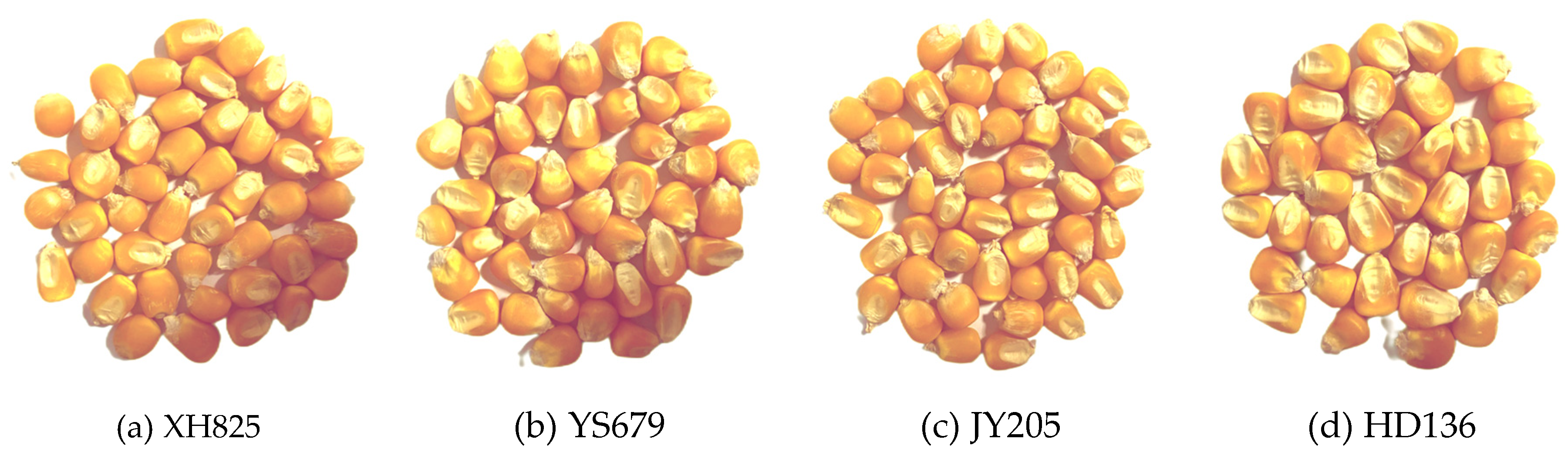
Figure 2.
Structure of hyperspectral image acquisition system.
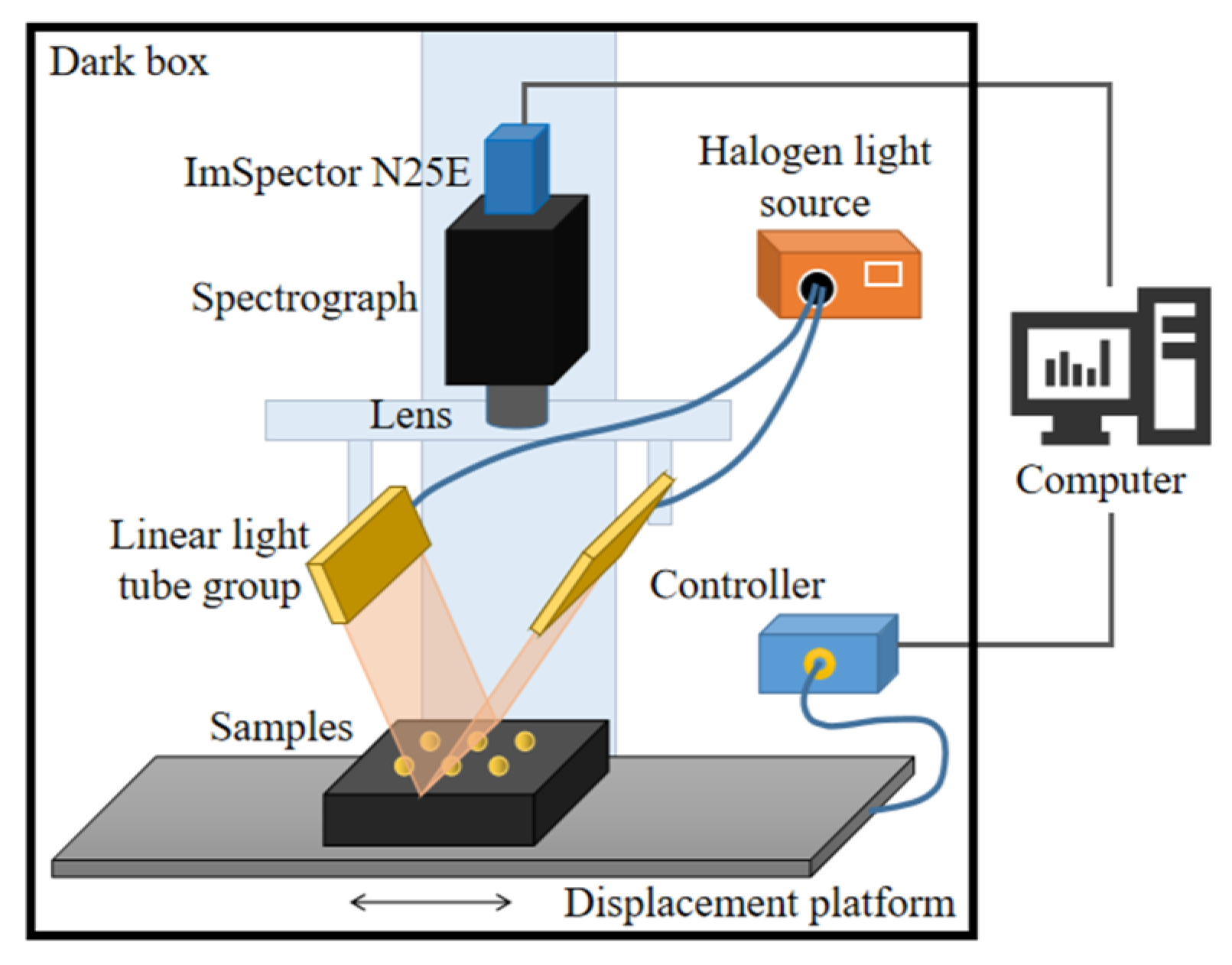
Figure 3.
Structure of Maize Seed.
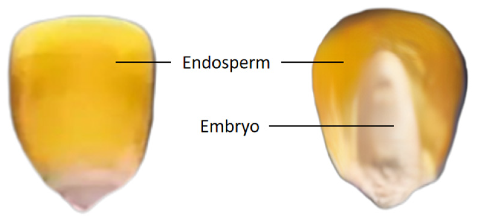
Figure 4.
Reflection spectra of maize kernel embryo, endospem and background.
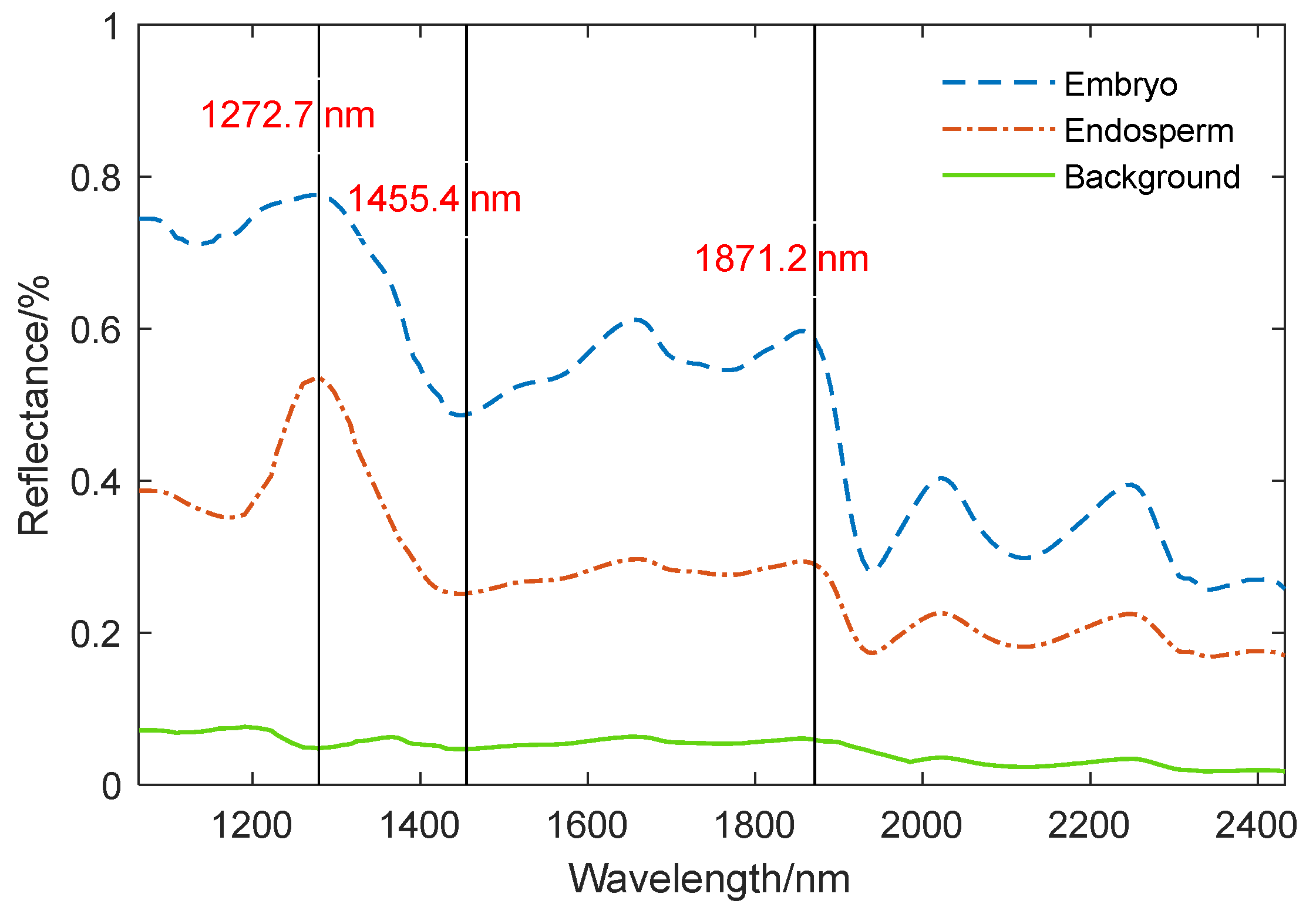
Figure 5.
Flowchart of extracting the maize kernel embryo.
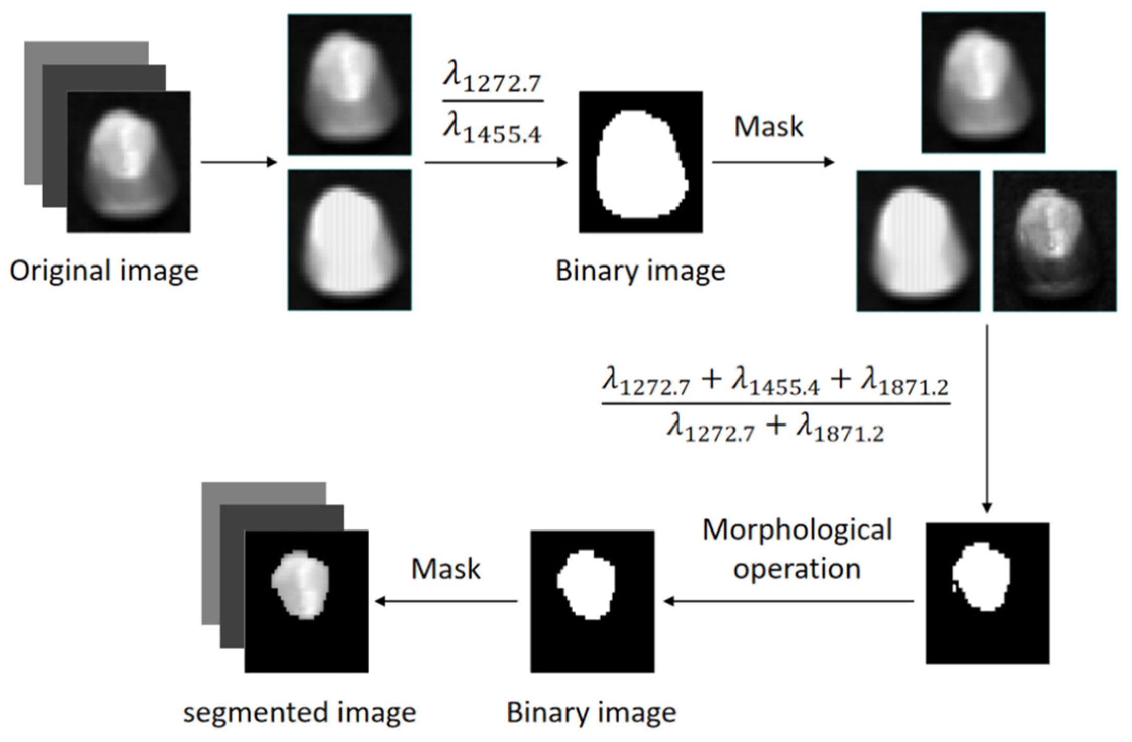
Figure 6.
Average spectral curve of embry.
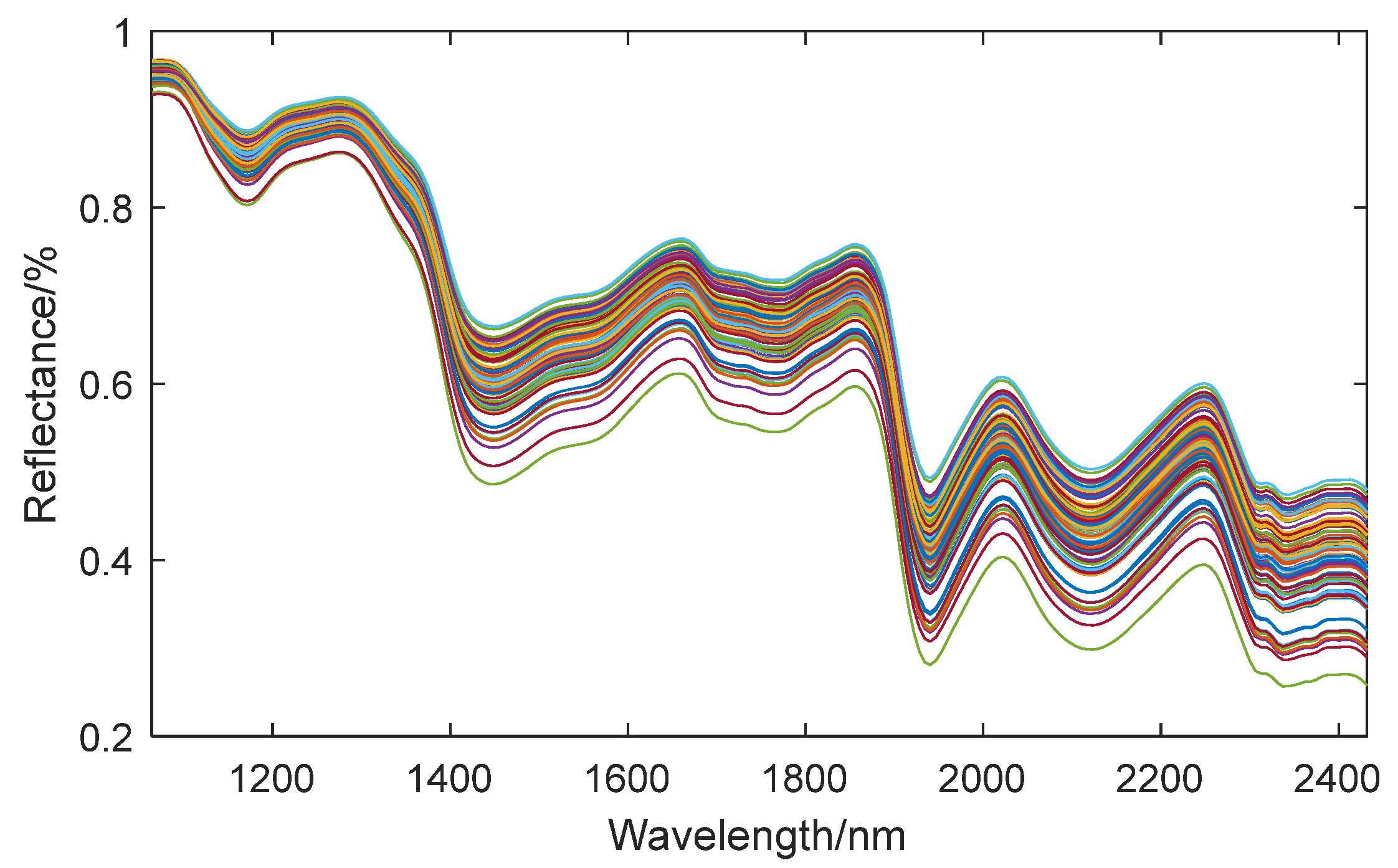
Figure 7.
Spectral curve after DT preprocessing.
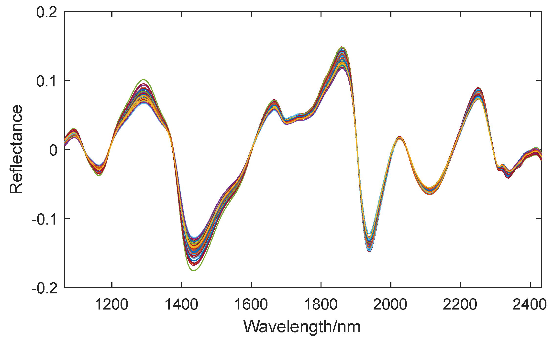
Figure 8.
Location of the characteristic wavelengths extracted by SPA for different components.
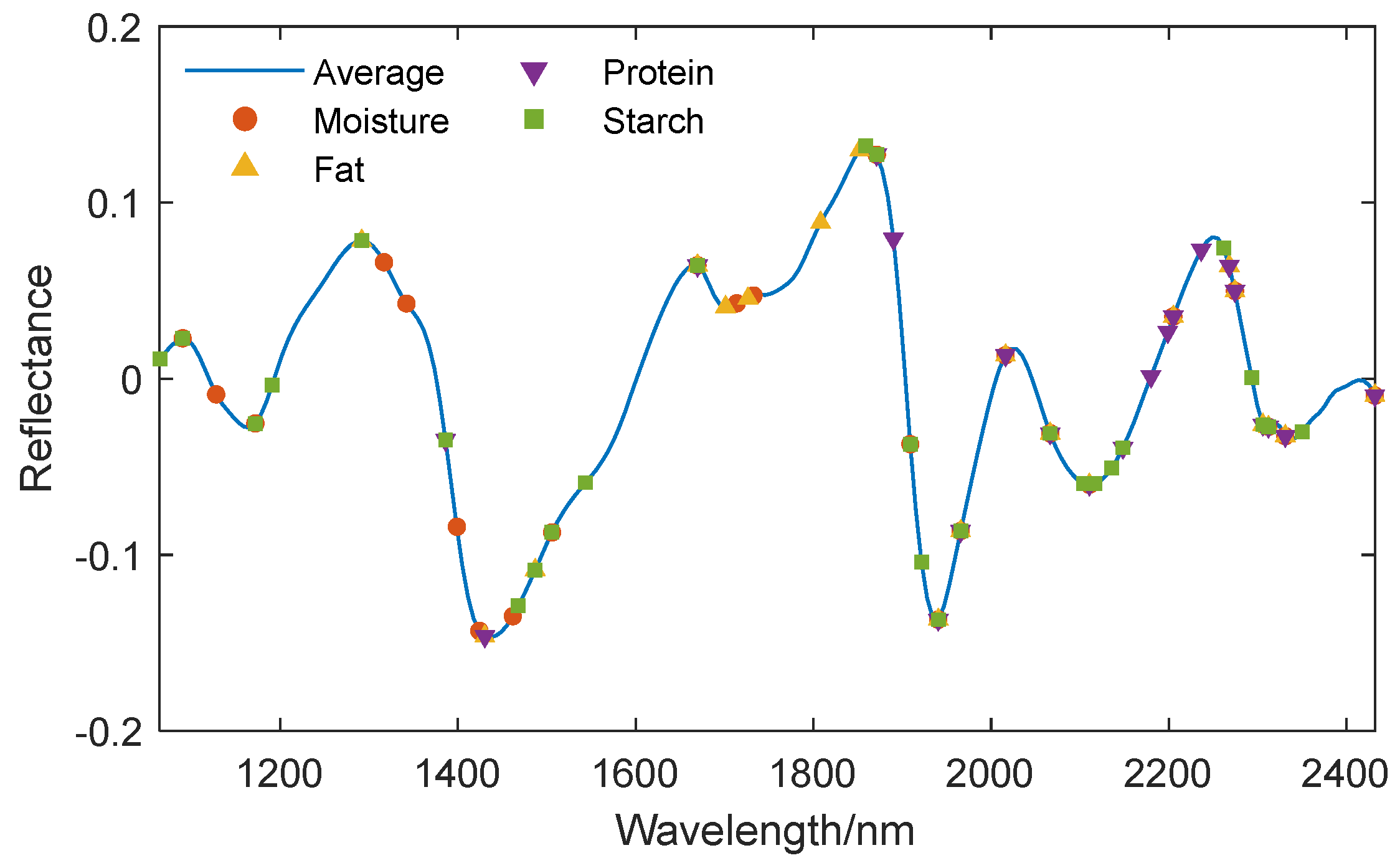
Figure 9.
Location of the characteristic wavelengths extracted by UVE for different components.
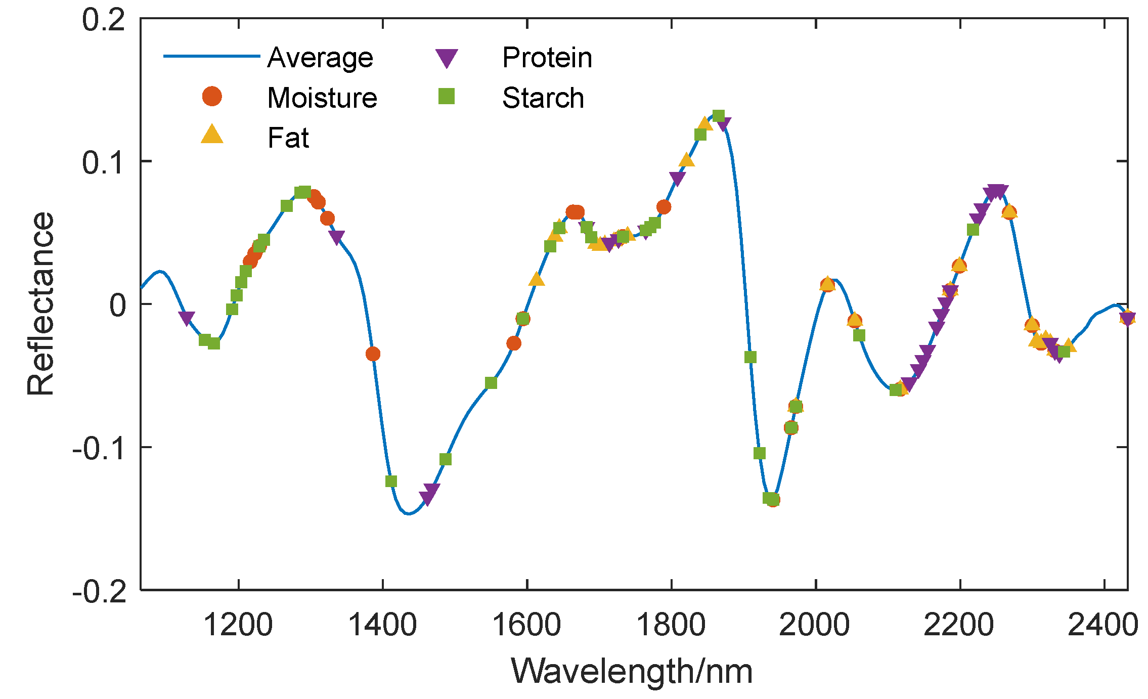
Figure 10.
Location of the characteristic wavelengths extracted by CARS for different components.
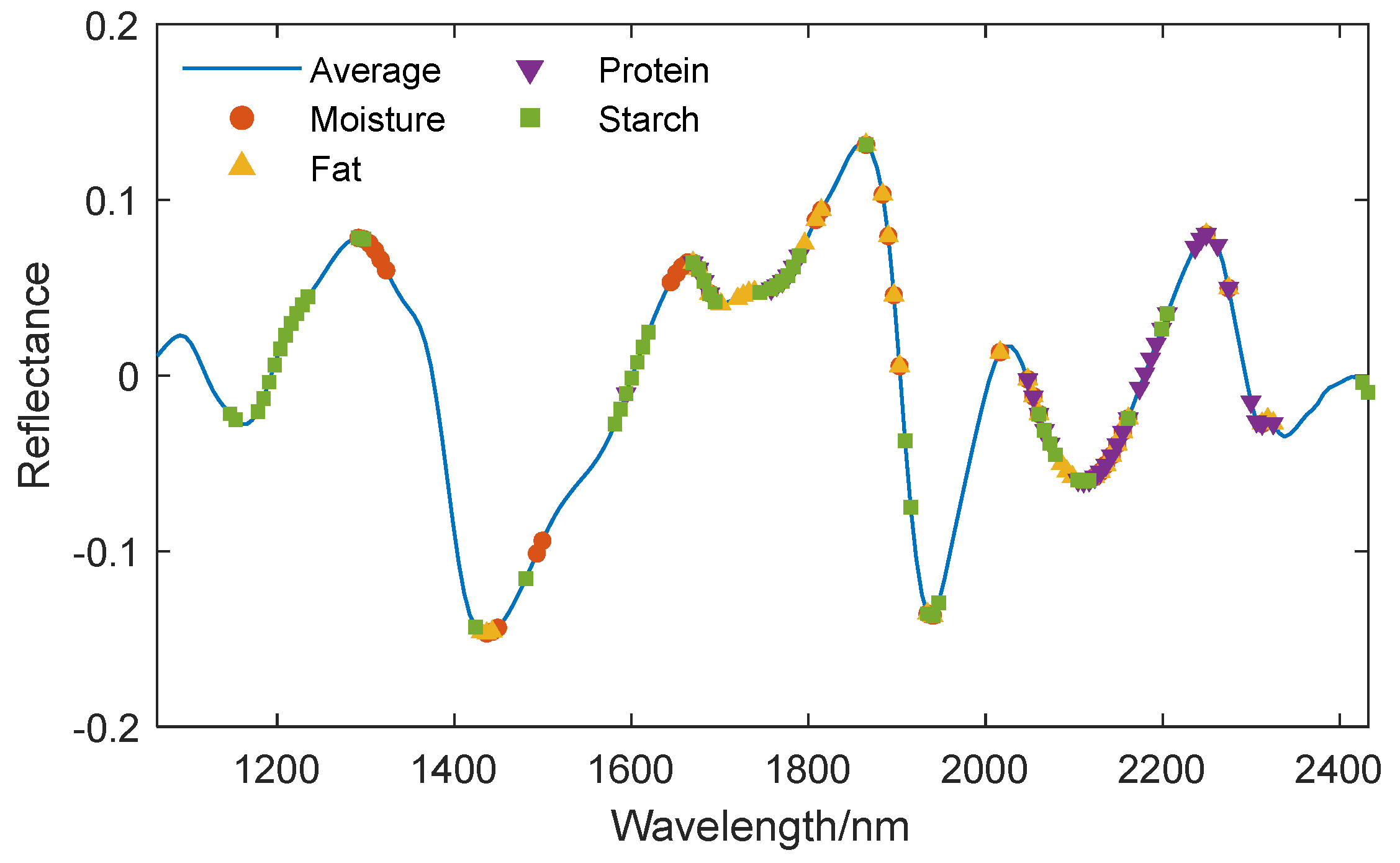
Figure 11.
Prediction results of moisture content detection models. (a) Prediction results of moisture content using full-band modeling; (b) Prediction results of moisture content based on SPA characteristic wavelength modeling; (c) Prediction results of moisture content based on UVE characteristic wavelength modeling; (d) Prediction results of moisture content based on CARS characteristic wavelength modeling.
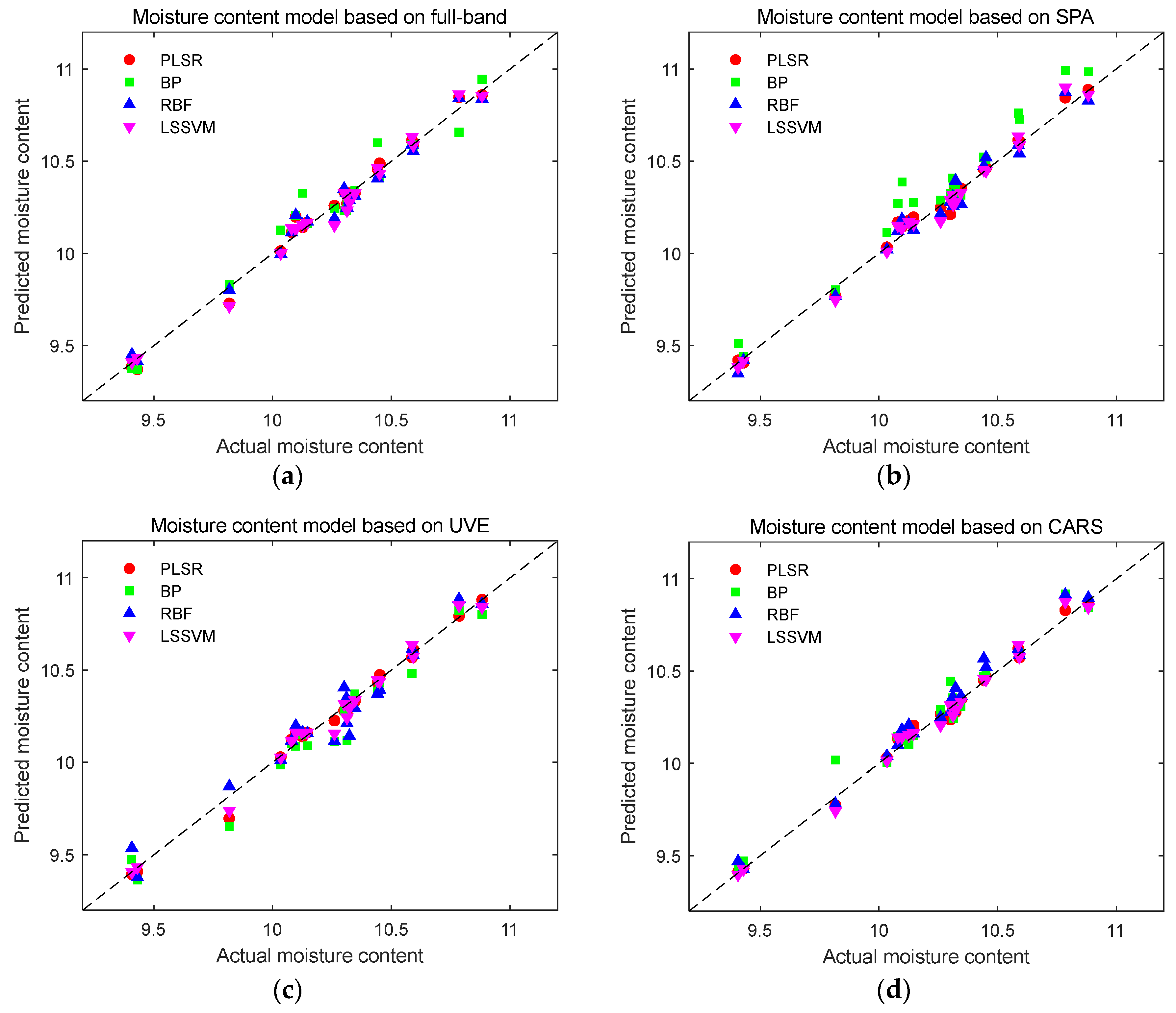
Figure 12.
Prediction results of fat content detection models. (a) Prediction results of fat content using full-band modeling; (b) Prediction results of fat content based on SPA characteristic wavelength modeling; (c) Prediction results of fat content based on UVE characteristic wavelength modeling; (d) Prediction results of fat content based on CARS characteristic wavelength modeling.
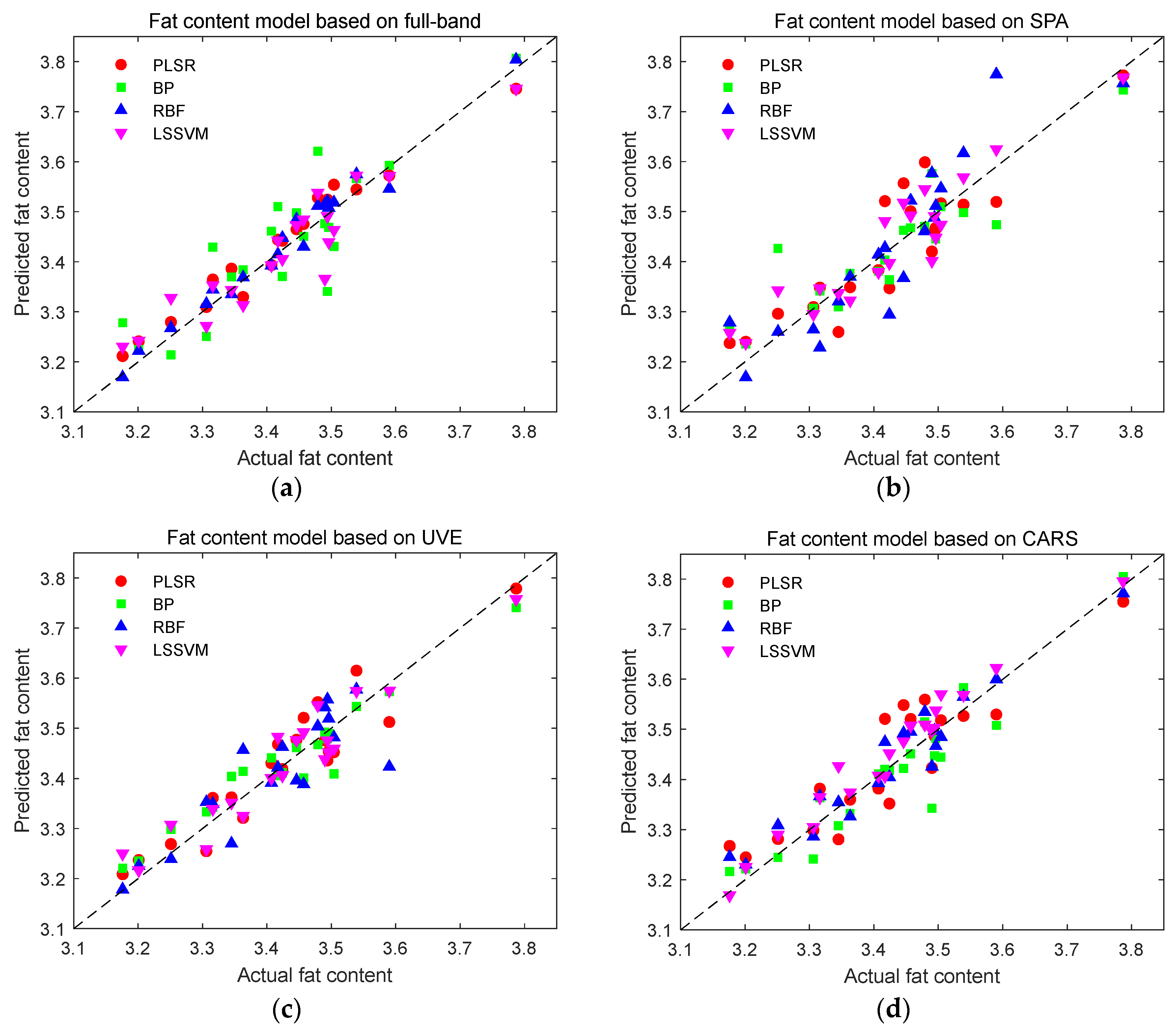
Figure 13.
Prediction results of protein content detection models. (a) Prediction results of protein content using full-band modeling; (b) Prediction results of protein content based on SPA characteristic wavelength modeling; (c) Prediction results of protein content based on UVE characteristic wavelength modeling; (d) Prediction results of protein content based on CARS characteristic wavelength modeling.
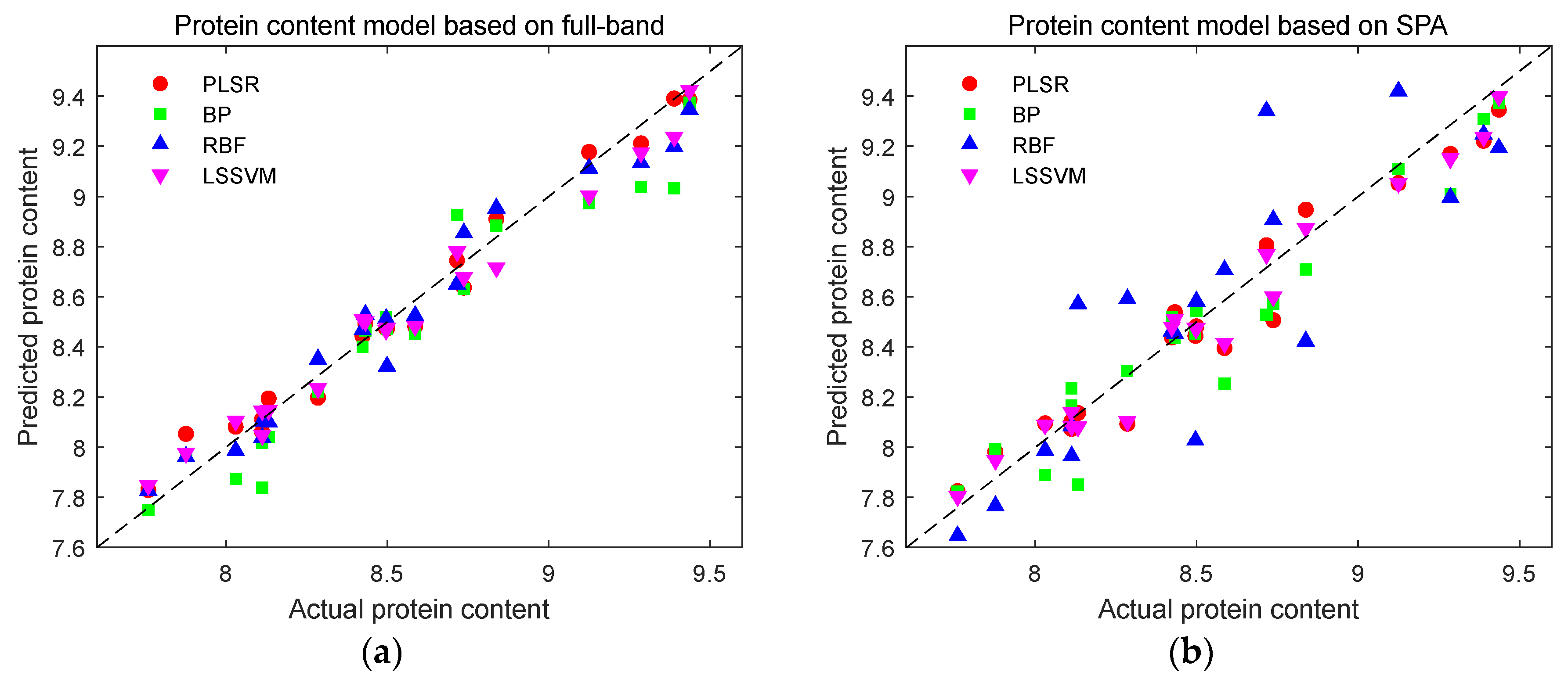
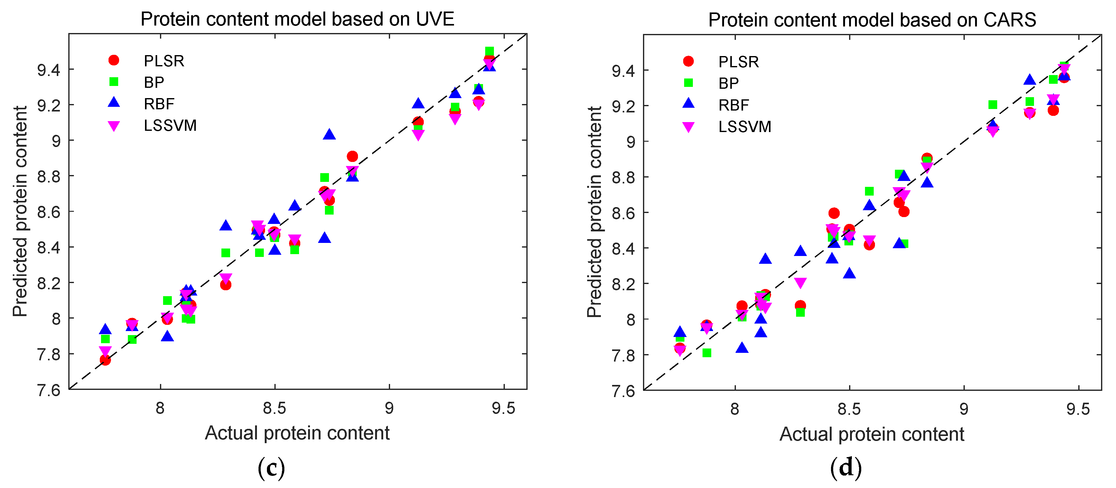
Figure 14.
Prediction results of starch content detection models. (a) Prediction results of starch content using full-band modeling; (b) Prediction results of starch content based on SPA characteristic wavelength modeling; (c) Prediction results of starch content based on UVE characteristic wavelength modeling; (d) Prediction results of starch content based on CARS characteristic wavelength modeling.
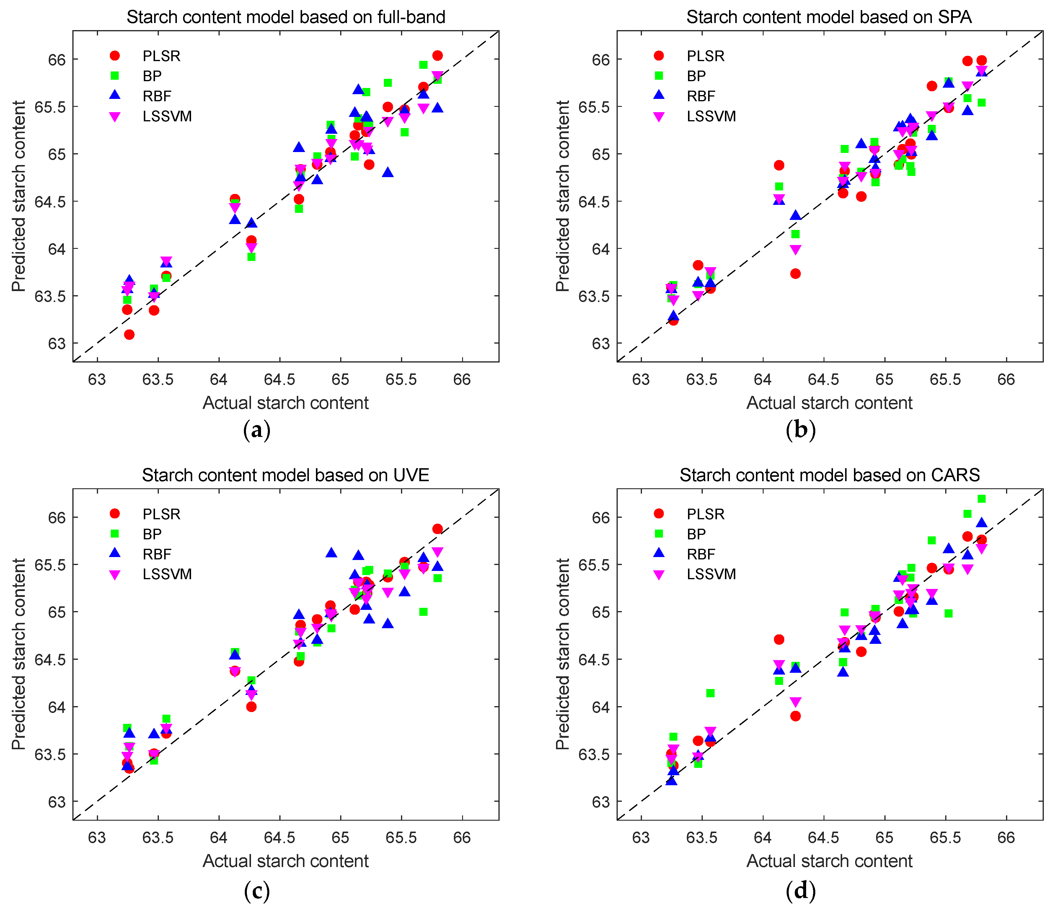

Table 1.
Statistics of the content of each component in the calibration set and prediction set of corn seed samples.
Table 1.
Statistics of the content of each component in the calibration set and prediction set of corn seed samples.
| Sample set | Number of samples | Parameter | Content/% | |||
|---|---|---|---|---|---|---|
| Moisture | Fat | Protein | Starch | |||
| Calibration set | 60 | Maximum | 10.993 | 3.832 | 9.711 | 66.472 |
| Minimum | 9.377 | 3.088 | 7.654 | 62.826 | ||
| Average | 10.233 | 3.523 | 8.692 | 64.691 | ||
| Standard deviation | 0.381 | 0.181 | 0.478 | 0.828 | ||
| Validation set | 20 | Maximum | 10.882 | 3.787 | 9.694 | 65.795 |
| Minimum | 9.407 | 3.176 | 7.759 | 63.246 | ||
| Average | 10.237 | 3.424 | 8.598 | 64.711 | ||
| Standard deviation | 0.368 | 0.137 | 0.538 | 0.778 | ||
Table 2.
Prediction results of PLSR models established based on different preprocessing methods.
| Component | Pretreatment method | PCs | Calibration set | Validation set | ||
|---|---|---|---|---|---|---|
| RMSEC | RMSEP | |||||
| Moisture | No pretreatment | 22 | 0.9928 | 0.0310 | 0.9748 | 0.0644 |
| MA | 27 | 0.9893 | 0.0378 | 0.9611 | 0.0800 | |
| SG | 27 | 0.9925 | 0.0317 | 0.9733 | 0.0662 | |
| NOR | 13 | 0.9831 | 0.0475 | 0.8227 | 0.1708 | |
| BC | 25 | 0.9925 | 0.0317 | 0.8720 | 0.1451 | |
| MSC | 11 | 0.9925 | 0.0317 | 0.8708 | 0.1458 | |
| SNV | 11 | 0.9925 | 0.0317 | 0.8720 | 0.1451 | |
| DT | 22 | 0.9997 | 0.0061 | 0.9906 | 0.0393 | |
| Fat | No pretreatment | 37 | 0.9052 | 0.0549 | 0.7483 | 0.0845 |
| MA | 23 | 0.8757 | 0.0628 | 0.6588 | 0.0984 | |
| SG | 28 | 0.8993 | 0.0565 | 0.7309 | 0.0874 | |
| NOR | 20 | 0.9809 | 0.0246 | 0.6982 | 0.0925 | |
| BC | 26 | 0.9937 | 0.0141 | 0.8275 | 0.0699 | |
| MSC | 13 | 0.9937 | 0.0141 | 0.8305 | 0.0693 | |
| SNV | 13 | 0.9937 | 0.0141 | 0.8275 | 0.0699 | |
| DT | 26 | 0.9985 | 0.0068 | 0.8706 | 0.0606 | |
| Protein | No pretreatment | 29 | 0.9563 | 0.1032 | 0.8995 | 0.1554 |
| MA | 36 | 0.9286 | 0.1320 | 0.8684 | 0.1778 | |
| SG | 40 | 0.9532 | 0.1069 | 0.8964 | 0.1578 | |
| NOR | 16 | 0.9933 | 0.0404 | 0.9265 | 0.1329 | |
| BC | 36 | 0.9981 | 0.0214 | 0.9365 | 0.1235 | |
| MSC | 13 | 0.9981 | 0.0214 | 0.9361 | 0.1239 | |
| SNV | 13 | 0.9981 | 0.0214 | 0.9365 | 0.1235 | |
| DT | 27 | 0.9994 | 0.0117 | 0.9535 | 0.1057 | |
| Starch | No pretreatment | 24 | 0.9162 | 0.2421 | 0.8249 | 0.3106 |
| MA | 29 | 0.8744 | 0.2964 | 0.7372 | 0.3806 | |
| SG | 19 | 0.9094 | 0.2517 | 0.8226 | 0.3127 | |
| NOR | 23 | 0.9942 | 0.0635 | 0.8793 | 0.2579 | |
| BC | 27 | 0.9980 | 0.0372 | 0.8986 | 0.2364 | |
| MSC | 20 | 0.9980 | 0.0373 | 0.8982 | 0.2369 | |
| SNV | 19 | 0.9980 | 0.0372 | 0.8986 | 0.2364 | |
| DT | 12 | 0.9979 | 0.0382 | 0.9145 | 0.2170 | |
Table 3.
The number of wavelengths selected based on different feature wavelength extraction algorithms.
Table 3.
The number of wavelengths selected based on different feature wavelength extraction algorithms.
| Algorithm | Moisture | Fat | Protein | Starch | Total |
|---|---|---|---|---|---|
| None | — | — | — | — | 218 |
| SPA | 24 | 14 | 10 | 24 | 51 |
| UVE | 27 | 14 | 25 | 35 | 105 |
| CARS | 41 | 15 | 39 | 53 | 89 |
Table 4.
Prediction results of various components in different models.
| Model | Feature wavelength extraction algorithm | ||||
|---|---|---|---|---|---|
| Moisture | Fat | Protein | Starch | ||
| PLSR | None | 0.9874 | 0.9472 | 0.9833 | 0.9532 |
| SPA | 0.9876 | 0.8017 | 0.9587 | 0.8692 | |
| UVE | 0.9900 | 0.8855 | 0.9792 | 0.9671 | |
| CARS | 0.9914 | 0.8215 | 0.9615 | 0.9395 | |
| BFNN | None | 0.9527 | 0.7398 | 0.9250 | 0.8906 |
| SPA | 0.8952 | 0.7994 | 0.9121 | 0.8941 | |
| UVE | 0.9522 | 0.9212 | 0.9701 | 0.8753 | |
| CARS | 0.9628 | 0.8680 | 0.9594 | 0.8621 | |
| RBFNN | None | 0.9847 | 0.9707 | 0.9696 | 0.8697 |
| SPA | 0.9804 | 0.7335 | 0.7495 | 0.9479 | |
| UVE | 0.9502 | 0.7903 | 0.9460 | 0.8387 | |
| CARS | 0.9744 | 0.9192 | 0.9346 | 0.9499 | |
| LSSVM | None | 0.9822 | 0.8799 | 0.9775 | 0.9453 |
| SPA | 0.9841 | 0.8696 | 0.9715 | 0.9520 | |
| UVE | 0.9857 | 0.9097 | 0.9768 | 0.9619 | |
| CARS | 0.9877 | 0.9344 | 0.9827 | 0.9592 | |
Disclaimer/Publisher’s Note: The statements, opinions and data contained in all publications are solely those of the individual author(s) and contributor(s) and not of MDPI and/or the editor(s). MDPI and/or the editor(s) disclaim responsibility for any injury to people or property resulting from any ideas, methods, instructions or products referred to in the content. |
© 2024 by the authors. Licensee MDPI, Basel, Switzerland. This article is an open access article distributed under the terms and conditions of the Creative Commons Attribution (CC BY) license (http://creativecommons.org/licenses/by/4.0/).
Copyright: This open access article is published under a Creative Commons CC BY 4.0 license, which permit the free download, distribution, and reuse, provided that the author and preprint are cited in any reuse.


