Submitted:
14 August 2024
Posted:
15 August 2024
You are already at the latest version
Abstract
The increasing demand for large-scale, high-frequency environmental monitoring has driven the adoption of satellite-based technologies for effective forest management, especially in the context of climate change. This study explores the potential of SAR for estimating the mass of harvesting residues, a significant component of forest ecosystems that impacts nutrient cycling, fire risk, and bioenergy production. The research hypothesizes that while the spatial distribution of residues remains stable, changes in moisture content—reflected in variations in the dielectric properties of the woody material—can be detected through SAR techniques. Two models, generalized linear model (GLM) and random forest (RF), were used to predict the mass of residues using interfer-ometric variables (phase, amplitude and coherence) as well as the backscatter signal from several acquisition pairs. The models provided encouraging results (R2 of 0.48 for GLM and 0.13 for RF), with acceptable bias and RMSE. We concluded that SAR data are feasible to predict the mass of harvesting residues and the findings could lead to improved monitoring and management of forest residues, contributing to sustainable forestry practices and enhanced bioenergy resource utilization.
Keywords:
Interferometry
; harvesting residues
; SAR
; sustainable forest management
1. Introduction
At the global level there has been an increasing demand for large-scale observations at high temporal frequency to monitor environmental changes and manage natural resources effectively, such as forests [1]. The increasing use of satellite-based technology offers a solution by enabling frequent, wide-area monitoring of forests, their status and biomass, along with other ecological parameters [2,3]. Traditional methods of forest monitoring, such as ground surveys and aerial photography, are labor-intensive and limited in spatial and temporal coverage [4]. Therefore, obtaining accurate and timely data is essential for informed decision-making, especially under the particularly crucial context of climate change and sustainable forest management.
Interferometric Synthetic Aperture Radar (InSAR) is a powerful remote sensing technique that generates high-resolution maps of surface deformation, topography, and other characteristics by analyzing the phase difference between two or more SAR images of the same area taken from slightly different positions or at different times [5]. Differential Interferometric SAR (DInSAR), an extension of InSAR, enhances this capability by comparing multiple SAR images over time to detect changes in the Earth's surface, providing detailed information on ground deformation and other dynamic processes [6].
DInSAR has become a valuable tool in environmental and forestry research, particularly since the BIOMASS mission, there is increasing interest in the use of this information for estimating forest biomass [7,8]. By capturing subtle changes in the forest canopy and ground structure, this technique can provide accurate measurements of forest height and volume [9], which are crucial for biomass estimation. Researchers leverage the sensitivity of SAR to the physical and dielectric properties of the observation objects to infer biomass from changes in signal phase and amplitude [10]. This method has been shown to be effective in various forest types and conditions, e.g. in the boreal forest of Canada [11] and Norway [12], in Brazilian Amazon [13] and tropical forests [14], making it an important technique for large-scale biomass monitoring and carbon stock assessment.
Harvesting residues, mainly consisting in branches and other non-commercial parts left on the ground after logging operations, are a significant component of forest ecosystems [15]. The role, presence and management of residues is a key factor for several reasons: they actively contribute to nutrient cycling within the forest [16], especially when it comes to influence Carbon and Nitrogen [17,18]; more to that, they also affect soil physical structure [19], biodiversity [20,21,22] and overall ecosystem health [23]. On the other hand, to reduce the impact and frequency of wildfires, the management of residues has helped to reduce the fire risk, as accumulated biomass can serve as fuel for wildfires [24]. At the same time, harvesting residues are a potential source of biomass for bioenergy production, an increasingly important element of renewable energy strategies [25,26].
Forest management procedures, such as clear-cutting, selective logging, and thinning, also depending on the machines and harvesting systems adopted, can generate varying amounts of harvesting residues [27]. The type and intensity of management practices influence the distribution and composition of residues, affecting subsequent decomposition rates and nutrient cycling.
Previous research on harvesting residues has primarily focused on field-based methods and statistical models to estimate the quantity and distribution of residues. Studies have explored various approaches at various scales and levels. Both Woo et al. [28] and Li et al. [29] have explored the possibility of integrating direct measurement from forest machinery during logging operations with allometric equations. Windrim et al. [30], on the other hand, developed an automated mapping of woody debris over recently harvested areas using UAV-borne data, high-resolution imagery and machine learning, and remote sensing techniques. However, these methods often face challenges in terms of scalability and accuracy, particularly over large and diverse forest landscapes.
The aim of this study is to understand the possibility to predict the quantity of harvesting residues over clear-felled areas for SAR data, in particular adopting InSAR and DInSAR techniques. The hypothesis is that along the observation period there will be little or no change in the residues spatial distribution (i.e., the geometry of the object), whereas most likely there will be changes in their properties, in particular the water content, that would be reflected in a variation of the dielectric constant of the woody material. Therefore only the change in moisture content will be investigated.
2. Materials and Methods
2.1. Study Area
The study area is part of an industrial forest plantation located in the KwaZulu-Natal province in South Africa (Figure 1). The complex topography of the province grants a varied and verdant climate: the area is characterized by a dry-winter humid subtropical climate, with warm summers and frequent rainfall. Winters are dry with high diurnal temperature variation, with possible light air frosts (South African Weather Service). The site, with a total surface of 17.54 ha, is divided into two parts which were both felled in the same period: the southern part has a surface of 7.34 ha, whereas the northern part is larger with a surface of 10.24 ha.
The species planted in the study area was Mexican weeping pine (Pinus patula Schiede ex Schltdl. & Cham.), hereafter identified as Pine. The harvesting operations were performed during February 2023, where the timber was mechanically felled by a harvester machine and then extracted and transported by forwarder to depot. The felling machine adopted was a Tigercat LH822D equipped with Log Max 7000XT head working with cut-to-length (CTL) technique, whereas the forwarder adopted was a Tigercat 1075C.
To better understand and inspect the area, the whole site was flown using a DJI Mavic Air 2S with a flying altitude of 65 m with 80% forward and 70% lateral overlap. The flight was performed in scattered cloud cover conditions, with Ground Control Points (GCP) positioned and recorded as well. The images were handled using a Structure-from-Motion (SfM) technique with Agisoft Metashape®, from which an orthomosaic was derived.
2.2. Field Data: Sampling Design and Residue Mass Estimation
The field measurements, used to estimate the harvesting residues mass, were first carried out in March 2023 in the southern part of the site, after the majority of the forwarding operations were completed and before the site was burnt and replanted at the end of October of the same year.
The sampling technique adopted was a line intercept sampling (LIS) method [31,32,33], used to estimate volumes and weights of downed woody material over completely clear-felled areas [34,35]. This technique considers residues on site to be randomly spread, with a random orientation under the sampling line and positioned horizontally, their circular shape, and the normal distribution of diameters.
Following the guidelines from Rizzolo [36], under each sampling line the diameter of every piece of woody debris was registered and classified in time lag classes (Table A 1). Each plot was composed of three sampling lines of 20 m each and organized as a perfect triangle with random orientation [37] (Figure 2); the number of triangles accounted for a total of 13 plots. For each triangle, the vertex positions were recorded using a GNSS system. The time lag division of woody material refers to the time required (in hours) for their moisture condition to fluctuate, Large woody debris, for example, will inherently take longer to dry out than finer material. According to this division, material finer than 76 mm in diameter belongs to fine woody debris (FWD) and larger material to coarse woody debris (CWD). The length has also been recorded for CWD larger than 203 mm.
Furthermore, 14 additional virtual plots were added across the area (using visual inspection in QGIS) to increase the information available for the training of the model, hereafter named “interpreted plots”, of which 8 were positioned in the northern part of the compartment. For each interpreted plot, the sampling design was similar to what was performed for the field plots: the plot corresponded to a perfect triangle with a side of 20 m and residues were sampled and digitized over the lines. The diameter for each piece was recorded and sorted in classes according to Table A 1. In particular, considering the resolution of the orthophoto (2.5 cm/pixel), it was possible to record residues with diameter with that dimension or higher.
The residue quantity estimation (Mg·ha-1) was performed for all categories of residues: for 1h, 10h, 100h, and 1000h classes, the Brown’s formula was used [34,35], described in Equation 1. Whereas for bigger elements, the ones falling in the 1000h+ class, the estimator was computed using the Woodall formula [35], expressed by Equation 3.
Where: 1.234 is a computational constant to convert the volume to m3/ha; n is the number of elements for each class; d is the average squared diameter for the class; c is the corrected slope (Equation 2); a is the correction coefficient for the position of the elements, equal to 1.13 for FWD and equal to 1 for CWD; SG is the specific gravity of the wood, in this case an average value of 0.575 was adopted (575 kg m-3); L is the length of the sampling line(s); kdecay is the decay coefficient as described in [35], in this case kdecay = 1 since the material was freshly cut; 10,000 are the square meters in 1 ha; yi is the volume for the single CWD piece and li is the length of the piece.
2.3. Satellite Data and Interferometric Processing
The Sentinel-1 mission included a constellation of two synchronous satellites where currently only one is still operating properly, equipped with a C-band synthetic aperture radar (SAR), enabling them to get acquisitions regardless of the weather. For this study, 4 dual polarization Sentinel-1 SAR C-band acquisitions were downloaded from the Alaska Satellite Facility (Copernicus Sentinel data 2023, processed by ESA), date of download: 13/07/2024. The images were acquired in the interferometric wide swath mode, containing data with a 250 km swath at 5 m by 20 m spatial resolution (single look, SLC), and captured in three sub-swaths using Terrain Observation with Progressive Scans SAR (TOPSAR). Each SLC-IW image contains single-look complex data, from which amplitude and phase can be computed for each polarization: the amplitude describing the strength of the signal and the phase the number of cycles modulo 2Pi of oscillation that the wave executes between the radar and the surface and back again.
In this study, we used a technique known as SAR Interferometry (InSAR), in which two images acquired from slightly different positions (i.e., separated by a spatial baseline) are used to obtain a three-dimensional image of the Earth’s surface.
In order to measure the changes of the surface, images need to be acquired at different times (i.e., using a temporal baseline), a technique denoted Differential SAR Interferometry (DInSAR). In this case, a reference image (“master”) was selected (in our case, 12/04/2023) to compare all following changes, whereas the others were defined as “slave” images (06/05/2023, 17/07/2023 and 09/10/2023) (Figure 3).
2.4. Pre-Processing of Satellite Images
The SAR images were first processed using the Sentinel Application Platform (SNAP) from ESA (ESA Copernicus Hub). First of all, the images were inspected and the first sub-swath was selected, as it alone contained the study area. Moreover, among the two polarizations (VH and VV), the proposed methodology relied only on VV-polarization since it has been proved to be more sensitive to surface moisture [38,39], whereas the cross-polarization signal is more sensitive to changes in the geometry and physical properties, such as the roughness.
The main steps of the following methodology are summarized in Figure 4. To better fulfill the aims of this research, images were coupled in short (April-May), medium (April-July) and long-period (April-October). For each pair of SLC-IW single-pol images, three explanatory variables were derived: the phase, the amplitude and the coherence using the interferometric approach and the intensity of the signal expressing the backscatter. The coherence provides a measure of similarity for each pixel ranging from 0 to 1, where 0 indicates that change did happen and 1 where no change has happened. First, the images were coregistered, their orbit corrected and stacked; then, the interferogram was computed. After the Topographic Phase removal, the interferogram was multilooked (number of looks = 3) and Goldstein phase filtered (coherence threshold = 0.4). After this, the DInSAR phase (∆φ), amplitude and coherence images were geocoded and exported.
To compute the backscatter, the VV-pol images were handled individually. After orbit and radiometric correction, the images underwent multilooking (number of looks = 3) and speckle filtering (sigma = 0.9). The images were terrain corrected and exported as γ0 images describing the backscatter coefficient normalized by the illuminated area projected into the look direction.
2.5. Feature Extraction and Prediction Model for Residue Mass Estimation
The following steps in the elaboration were performed using R [40] and RStudio environment (R version 4.4.1; RStudio 2024.04.2+764 "Chocolate Cosmos"). After the pre-processing, the ∆φ, amplitude, coherence and γ0 images were stacked together and handled as raster, using the terra package [41]. The plots were paired with the mean quantity value obtained by averaging the estimations from their sample lines. The shapefile containing this information was used to extract the mean value from the stacked backscatter and then converted to data frame.
The data frame was used to feed two models: a generalized linear model (GLM) and a Random Forest model (RF). In the first case, the application of a linear model also had the intention to find possible correlations between the variables and to underline possibly significant variables available in the data frame. The RF model used is a machine learning algorithm built with the R package randomForest [42], with forest size of 500 trees (ntree = 500). All variables were used to initially feed the model, adequately setting the split decision parameter (mtry), and training and testing was performed using a leave-one-out cross-validation (LOOCV) procedure. The RF model was then iteratively adjusted by excluding the variables that reported a negative importance score.
2.6. Coherence Difference Analysis
To better gain insights on the results, a separate analysis was performed by considering the coherence values, comparing each image pair and by computing the differences between the pairings. Coherence (ϒ) values are calculated at pixel level and range from 0 to 1; a value of 1 indicates no alteration in the scattering properties between images [43]. However, when the observed surface changes, the complex backscatter is impacted causing a decrease in coherence, which is known as decorrelation. This approach moves from already established coherence difference analysis (CDA) methods [44] but still follows the same purpose, to define and to investigate the source of decorrelation. Consistent with [45] the interferometric coherence is affected by three main factors of decorrelation: radar thermal noise decorrelation (ϒN), geometric decorrelation (ϒG), and temporal decorrelation (ϒT). Considering that all images were acquired by the same antenna, it is reasonable to assume that the variation in thermal noise between images will not influence the coherence decorrelation [43] The geometric decorrelation, on the other hand, is highly influenced by the perpendicular baseline; if this parameter is major than the critical value, then ϒG becomes 0, causing maximum decorrelation [46]. Finally, the temporal decorrelation is the one that would contribute the most since the loss in coherence is mainly due to changes in the object's properties (i.e., geometry structure and dielectric properties).
2.7. Validation Assessment
Both models were validated by using the field plots as reference by comparing the predicted values against the estimates obtained through volume calculation. In this case, two indicators were considered: the squared Pearson index (R2) to evaluate the correlation between the field values and the predicted, and the Root Mean Squared Error (RMSE) to assess the model performance. At the end, the model was used to predict the residues mass distribution throughout the study site.
To further evaluate the goodness of the produced residues estimations and mapping, the field plots were also visually inspected, and the diameter of the material was registered, with the residues mass computed. After this, the bias and RMSE were computed.
3. Results
3.1. Field and Interpreted Plots Residues Quantity
The estimated quantities per hectare and per plot surface are reported in Table 1. Considering the average values, it can be shown that the Interpreted plots have higher values in both quantities per hectare and per plot surface (+113% compared to the field measurements). Nonetheless, if considering the total mass for each plot, the two series report comparable information (Table A 2 and Table A 3).
3.2. Coherence Difference Analysis
The coherence differences were computed for each image pair and between pairs (Figure 5). For the first pair (April-May), the coherence values were estimated between 0.036 and 0.793 (mean = 0.302; standard deviation = 0.13), whereas for the second pair (April-July), the values ranged from a minimum of 0.031 to 0.779 (mean = 0.258; standard deviation = 0.102). The last pair, April-October, showed coherence values between 0.037 and 0.679 (mean = 0.249; standard deviation = 0.097). The observed difference in the statistics results over time (short, medium and long period) denote an important decorrelation process between acquisitions. The coherence difference maps showed values between −0.531 and 0.555 (mean = −0.044; standard deviation = 0.152) for Figure 5C map, while the values reported in Figure 5E ranged from −0.651 to 0.482 (mean = −0.053; standard deviation = 0.156).
3.3. Prediction Models and Validation Assessment
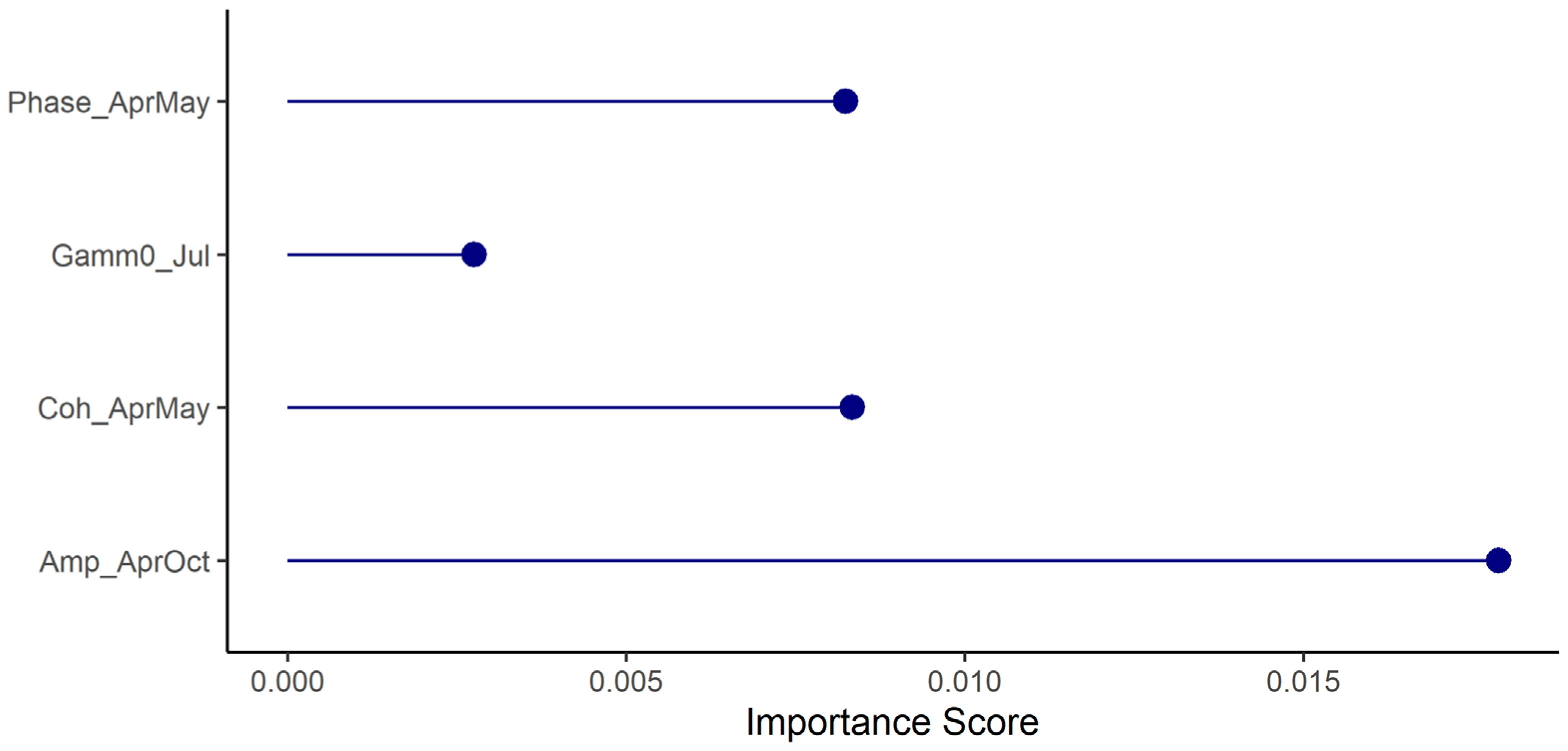
The results for the GLM and RF models are shown in Figure 6, with the distinction between field plots and interpreted plots. In this case, the GLM model have used all the variables (Table A 5) with only one showing significant contributions at the end (p < 0.1), i.e. the phase from the April-May interferogram. The variables feeding the RF model, on the other hand, were filtered based on their importance score using only variables with a positive score (Figure A 1): in this case, the variables reaching the highest scores are the amplitude from the April-October interferogram and the phase from April-May, with also the contribution of the Coherence April-May and the γ0 from July; the rest of the variables show the same importance score. Overall, the GLM model performed better in terms of both R2 and RMSE compared to RF. In the validation process, i.e. by considering only the field plots, the GLM model outperformed RF again (Figure 7).
For the bias assessment, the field plots have been inspected and interpreted, with the resulting volumes reported in Table A 5 and the error indices per single plot values (Mg) in Table 2. In this case, the errors computed underline how the residues estimated with the visual interpretation method are biased, on average, with a -0.05 Mg when considering just the CWD components (1000h and 1000h+ classes), and 0.14 Mg when considering all classes of material. The RMSE is lower than the one provided by both the GLM and RF models.
The representation of the residue distribution over the study area is then reported in Figure 8, with respect to the single plots quantity. In this case, the heat map built with the GLM model tends to represent all the spectrum of values, whereas the RF model tends to represent values converging towards the mean of the distribution. Regardless of the accuracy of the model used to depict such spatial representation, this tendency can be seen by using the plots values as references.
4. Discussion
This paper aimed to evaluate the possibility of using SAR data techniques (InSAR and DInSAR) to quantify the mass of harvesting residues left in clear-felled areas. The proposed approach was to compare two prediction models and evaluate their goodness-of-fit (R2), RMSE, and bias. This paper offers an innovative approach to estimate residues quantities more conveniently than physically weighing their mass.
The coherence difference analysis assumed that the presence of harvesting residues in clear-felled areas would be less stable over time than the surrounding solid soil (due to decomposition processes, residue pile volumes gradually collapsing to a solid ground layer etc.). Hence, residues would decorrelate more (measured as decreasing coherence) as time passes. The variation in dielectric constant was assumed to be lower for the surrounding clear-cut plantation, and hence present only smaller changes in the backscatter between SAR images. The perpendicular baselines ranged from -117 m to 80 m, which is a bit large for the sensitivity we aimed for. Nevertheless, the loss of coherence was useful in our predictions.
In the short term , the coherence exhibits higher values inside the harvesting area with more variations outside the perimeter, where the trees are still standing, as also reported by Akbari et al. [47], whereas the coherence gradually decreases with time, resulting in values close to 0. Considering the absence of inclement weather conditions throughout the time of observation, the changes in coherence in the short term are likely due to changes in volume scattering and changes of the dielectric constant throughout the drying process; changes in the surrounding trees are more likely related to fluctuations in the crown water content, due to the SAR operating at C-band [48]. These assumptions are also supported by the coherence differences , where lower changes are noticed outside the logged area (Figures 5C and 5E). Some of these findings were also noted when developing the linear prediction models, where the relation and contribution of various variables were studied. For example, in the GLM model the variables with the highest significance came from the short period interferogram (i.e., the April-May interferogram), that is also exhibiting higher variation in coherence values. On the other hand, the RF model prefers the phase difference between April and May, but also the amplitude from April-October (long term) and the γ0 from July.
The magnitude of residue masses estimated through the field survey are comparable with the values available in the literature for the species considered [37,49]. The higher residue mass values of the interpreted plots (+113% compared to the field plots) can be due to the influence of several factors. First of all, the interpretation and visual inspection of the logging area by the means of aerial photogrammetry: although available with fairly high resolution (2.5 cm/pixel), still the orthomosaic used for the visual assessment of the residues did not allow for the inspection and registration of the smaller woody material, with diameters lower than 3 cm (i.e., 1h and 10h classes). This could be reflected in the average quantities per plot that are higher in the interpreted plots compared to the field ones. Moreover, whereas the field survey also considers stumps, the visual inspections do not, therefore further reducing the CWD material estimations. A similar issue can be found also in [30], although using a different system for manual annotation. Second, the presence of residue piles in the area does not allow for an optimal visual annotation of material from QGIS, since it would be possible to register only the diameter of the elements on the very top of the pile, whereas with the field survey some material also from the deeper layer can be registered. Therefore, the volumes or masses considered results in different values, also for the same plots, as exposed by the bias evaluation (-0.05 Mg and 0.14 Mg, for CWD and FWD+CWD considered material).
Nevertheless, there are different factors and limitations to consider for this study and the proposed methodology. The main principle of the DInSAR technique adopted is that it allows for the retrieval of any changes on the surface of the area investigated, through the scatter of the beam signal; the rougher the object, the more scatter it should produce.
- Overall, this study investigated only the use of VV-polarization acquisitions, based on previous literature, considering any major detectable changes due to moisture variation in the residues and piles;
- A second general limitation is regarding the object of the investigation, the harvesting residues. Although not individually detectable using the SAR pixel size (10 x 10 m), they can be addressed in piles, providing a large (on average, 5 meters wide and 1.5 meters tall, at maximum), complex and rough object, when performing this kind of research. However, obtaining precise information of pile masses and volumes is still challenging, both with field measurements and remote sensing-based techniques [49,50,51];
- A topic more related to the prediction models is the number of available plots used to feed the model and its design. To increase the R2 of the results and their robustness, it would have been necessary to have more field observations for both GLM and RF models. In fact, both models can be easily exposed to dataset with a limited number of observations, in particular RF [52], therefore more in-field observation are preferrable;
- The analysis of coherence provided insightful information about the signal scattering and its changes throughout the monitored period. Although minimized, different sources of decorrelation might have still played a role in the obtained results, especially the geometric decorrelation. Moreover, to properly address the volume scattering, the proposed methodology featured also the backscatter signal γ0, but saw limited contribution from the majority of them (Figure A 1). In this case, the possible addition of VH-polarization backscatter could add complexity to the response, delivering a more comprehensive output.
5. Conclusions
The paper evaluated the possibility for SAR data to predict the quantity of harvesting residues over clear-felled areas, performed over a study area of a pine plantation in South Africa. The models predictions provided results with an R2 index of 0.47 and 0.13 for GLM and RF, respectively, when using all plots, and 0.23 and 0.006 when using only the field plots. The RMSE stabilized between 0.20-0.28 Mg. Overall, the bias regarding the interpretation of the woody material ranged between -0.05 and 0.14 Mg. Nevertheless, we can positively affirm that, even at this stage and with the limitations listed above, it is possible to derive harvesting residues mass from SAR data handled with InSAR and DInSAR techniques.
This information could be suitable to forest owners and managers for the possible retrieval of material to convoy to bio-energy producing plants, or to provide an indirect estimation of possible C-stock in woody material to help industrial companies to account for carbon or reduce their impact on biogeochemical cycles and nutrient fluxes in the re-establishment of timber plantations and the use of fertilizers.
Future research should address the necessity of defining a suitable number of plots or sampling design to derive residues information and train/test any prediction model. Moreover, the possibility of having different observations on different sites at the same time could be interesting to explore to address local variability between sites and/or species.
Author Contributions
Conceptualization, A.U. and S.G.; methodology, A.U. and H.J.P.; investigation, data curation and data collection, A.U., and B.T.; software and validation, A.U. and H.J.P.; formal analysis, B.T.; writing—original draft preparation, A.U.; writing—review and editing, A.U., S.G., H.J.P., and B.T.; visualization, A.U., S.G., H.J.P., and B.T.; supervision, S.G. All authors have read and agreed to the published version of the manuscript.
Funding
The study was supported by the European Union’s HORIZON 2020 research and innovation programme under the Marie Skłodowska Curie grant agreement N° 778322 and by the Agritech National Research Center and received funding from the European Union Next-Generation EU (PIANO NAZIONALE DI RIPRESA E RESILIENZA (PNRR) – MISSIONE 4 COMPONENTE 2, INVESTIMENTO1.4—D.D. 103217/06/2022, CN00000022) within the Task 4.1.4 (Spoke4).
Data Availability Statement
The raw data supporting the conclusions of this article will be made available by the authors on request.
Acknowledgments
The authors would like to thank Simon Ackermann, Hilton Brown and the whole staff at Merensky Timbers’ Weza plantation for the help provided during the field campaign.
Conflicts of Interest
The authors declare no conflicts of interest.
Appendix A

Table A 1.
Time lag class distribution, with diameter (D) thresholds, and category for forest residues (FWD - fine woody debris, CWD - coarse woody debris) [34,36].
| Class | D min (mm) | D max (mm) | Category |
|---|---|---|---|
| 1h | 0 | 6 | FWD |
| 10h | 6 | 25 | |
| 100h | 25 | 76 | |
| 1000h | 76 | 203 | CWD |
| 1000h+ | >203 |
Table A 2.
Average mass value (Mg ha-1) for residues (FWD - fine woody debris, CWD - coarse woody debris) for the field plots and divided for each class. Standard deviation is also reported in brackets.
Table A 2.
Average mass value (Mg ha-1) for residues (FWD - fine woody debris, CWD - coarse woody debris) for the field plots and divided for each class. Standard deviation is also reported in brackets.
| Plot | FWD | CWD | Average mass | |||
|---|---|---|---|---|---|---|
| 1h | 10h | 100h | 1000h | 1000h+ | ||
| 1 | 0.63 | 9.48 | 21.20 | 11.54 | 43.31 | 18.32 |
| 2 | 0.51 | 8.52 | 19.37 | 46.68 | 56.44 | 27.72 |
| 3 | 0.45 | 7.23 | 22.45 | 16.19 | 36.38 | 17.45 |
| 4 | 0.52 | 7.72 | 14.40 | 34.69 | 21.00 | 16.19 |
| 5 | 0.49 | 7.02 | 9.62 | 9.34 | 23.80 | 10.65 |
| 6 | 0.52 | 9.56 | 15.55 | 11.61 | 29.18 | 14.02 |
| 7 | 0.52 | 8.80 | 18.51 | 27.83 | 75.66 | 28.16 |
| 8 | 0.57 | 8.43 | 19.54 | 23.23 | 3.79 | 11.21 |
| 9 | 0.61 | 10.98 | 21.28 | 20.88 | 22.74 | 15.87 |
| 10 | 0.47 | 6.29 | 14.76 | 48.61 | 30.35 | 20.86 |
| 11 | 0.60 | 11.68 | 25.37 | 32.42 | 43.13 | 23.72 |
| 12 | 0.53 | 5.74 | 15.76 | 20.81 | 50.07 | 19.84 |
| 13 | 0.59 | 9.18 | 22.29 | 18.56 | 27.87 | 16.39 |
| Average | 0.54 (0.13) | 8.51 (3.63) | 18.47 (6.55) | 24.80 (19.29) | 35.67 (47.70) | 18.49 (5.30) |
Table A 3.
Average mass value (Mg ha-1) for residues (FWD - fine woody debris, CWD - coarse woody debris) for the interpreted plots and divided for each class. Standard deviation is also reported in brackets.
Table A 3.
Average mass value (Mg ha-1) for residues (FWD - fine woody debris, CWD - coarse woody debris) for the interpreted plots and divided for each class. Standard deviation is also reported in brackets.
| Plot | FWD | CWD | Average mass | |||
|---|---|---|---|---|---|---|
| 1h | 10h | 100h | 1000h | 1000h+ | ||
| 14 | - | - | 17.49 | 98.67 | 6.25 | 40.81 |
| 15 | - | - | 14.06 | 130.97 | 7.39 | 50.81 |
| 16 | - | - | 21.95 | 102.26 | 51.65 | 58.62 |
| 17 | - | - | 12.01 | 93.29 | 0.00 | 35.10 |
| 18 | - | - | 19.55 | 91.50 | 0.00 | 37.02 |
| 19 | - | - | 6.86 | 80.73 | 0.00 | 29.20 |
| 20 | - | - | 7.89 | 93.29 | 41.01 | 47.40 |
| 21 | - | - | 1.03 | 8.20 | 28.73 | 12.65 |
| 22 | - | - | 11.32 | 123.79 | 16.24 | 50.45 |
| 23 | - | - | 11.32 | 104.06 | 20.21 | 45.19 |
| 24 | - | - | 3.09 | 138.14 | 12.02 | 51.09 |
| 25 | - | - | 3.43 | 48.44 | 20.49 | 24.12 |
| 26 | - | - | 2.74 | 89.70 | 7.39 | 33.28 |
| 27 | - | - | 4.80 | 96.88 | 3.83 | 35.17 |
| Average | - | - | 9.82 (6.43) | 92.85 (31.65) | 15.37 (15.27) | 39.95 (11.92) |
Table A 4.
Average interpreted mass value (Mg ha-1) for residues (FWD - fine woody debris, CWD - coarse woody debris) for the field plots and divided for each class. Standard deviation is also reported in brackets.
Table A 4.
Average interpreted mass value (Mg ha-1) for residues (FWD - fine woody debris, CWD - coarse woody debris) for the field plots and divided for each class. Standard deviation is also reported in brackets.
| Plot | FWD | CWD | Average mass | |||
|---|---|---|---|---|---|---|
| 1h | 10h | 100h | 1000h | 1000h+ | ||
| 1 | - | - | 28.09 | 5.37 | 5.21 | 13.81 |
| 2 | - | - | 20.63 | 32.38 | 5.21 | 19.41 |
| 3 | - | - | 24.49 | 5.41 | 49.12 | 26.34 |
| 4 | - | - | 26.01 | 50.12 | 14.48 | 30.20 |
| 5 | - | - | 14.75 | 19.73 | 6.81 | 13.76 |
| 6 | - | - | 29.59 | 30.60 | 17.32 | 26.98 |
| 7 | - | - | 23.04 | 44.96 | 3.83 | 23.94 |
| 8 | - | - | 21.58 | 46.58 | 0.00 | 22.72 |
| 9 | - | - | 28.12 | 35.88 | 28.10 | 30.70 |
| 10 | - | - | 13.71 | 71.72 | 3.83 | 29.75 |
| 11 | - | - | 19.50 | 62.64 | 4.27 | 30.17 |
| 12 | - | - | 14.37 | 71.58 | 14.81 | 33.59 |
| 13 | - | - | 23.67 | 52.03 | 0.00 | 25.23 |
| Average | - | - | 22.91 (5.80) | 40.69 (21.11) | 11.77 (13.24) | 25.13 (6.06) |
Table A 5.
Summary of GLM model, with variables used and significance based on computed t value.
| Estimate Std. | Error | t value | Pr(> |t|) | |
|---|---|---|---|---|
| (Intercept) | 43.93124 | 48.15602 | 0.912 | 0.3771 |
| Coherence_AprMay | 0.04598 | 0.74621 | 0.062 | 0.9517 |
| Coherence_AprJul | -0.02640 | 0.72589 | -0.036 | 0.9715 |
| Coherence_AprOct | -0.09081 | 0.88356 | -0.103 | 0.9196 |
| Gamma0_Apr | -0.08089 | -0.10316 | -0.7840 | 0.4460 |
| Gamma0_May | 0.08588 | 0.07806 | 1.100 | 0.2898 |
| Gamma0_Jul | NA | NA | NA | NA |
| Gamma0_Oct | 0.08323 | 0.09982 | 0.834 | 0.4184 |
| Amp_AprMay | -2.56988 | 1.49622 | -1.718 | 0.1079 |
| Amp_AprJul | -0.08817 | 1.20188 | -0.073 | 0.9426 |
| Amp_AprOct | 0.87675 | 1.14049 | 0.769 | 0.4548 |
| Phase_AprMay * | -0.47721 | 0.24671 | -1.934 | 0.0735 |
| Phase_AprJul | 0.02123 | 0.04168 | 0.509 | 0.6185 |
| Phase_AprOct | -0.02152 | 0.05746 | -0.375 | 0.7136 |
| Residual standard error: 0.2751 on 14 degrees of freedom | ||||
| Multiple R-squared: 0.4666, Adjusted R-squared: 0.009482 | ||||
| F-statistic: 1.021 on 12 and 14 DF, p-value: 0.4798 | ||||
Signif. codes: 0 ‘***’ 0.001 ‘**’ 0.01 ‘*’ 0.05 ‘.’ 0.1 ‘ ’ 1
Figure A1.
Importance score for the variables used in the final RF model. The Mean of squared residual computed by the model was 0.069 Mg with a 9.42% of variance explained.
Figure A1.
Importance score for the variables used in the final RF model. The Mean of squared residual computed by the model was 0.069 Mg with a 9.42% of variance explained.
References
- Achat, D.L., Deleuze, C., Landmann, G., Pousse, N., Ranger, J., Augusto, L., 2015. Quantifying consequences of removing harvesting residues on forest soils and tree growth - A meta-analysis. For Ecol Manage. [CrossRef]
- Akbari, V., Solberg, S., 2022. Clear-Cut Detection and Mapping Using Sentinel-1 Backscatter Coefficient and Short-Term Interferometric Coherence Time Series. IEEE Geoscience and Remote Sensing Letters 19. [CrossRef]
- Bispo, P.D.C., Pardini, M., Papathanassiou, K.P., Kugler, F., Balzter, H., Rains, D., dos Santos, J.R., Rizaev, I.G., Tansey, K., dos Santos, M.N., Spinelli Araujo, L., 2019. Mapping forest successional stages in the Brazilian Amazon using forest heights derived from TanDEM-X SAR interferometry. Remote Sens Environ 232, 111194. [CrossRef]
- Bose, T., Vivas, M., Slippers, B., Roux, J., Kemler, M., Begerow, D., Witfeld, F., Brachmann, A., Dovey, S., Wingfield, M.J., 2023. Retention of post-harvest residues enhances soil fungal biodiversity in Eucalyptus plantations. For Ecol Manage 532, 120806. [CrossRef]
- Bousbih, S., Zribi, M., Lili-Chabaane, Z., Baghdadi, N., El Hajj, M., Gao, Q., Mougenot, B., 2017. Potential of Sentinel-1 Radar Data for the Assessment of Soil and Cereal Cover Parameters. Sensors 2017, Vol. 17, Page 2617 17, 2617. [CrossRef]
- Brown, J.K., 1974. Handbook for Inventorying Downed Woody Material, USDA For. Serv. Gen. Tech. Rep.
- Buchhorn, M., Lesiv, M., Tsendbazar, N.E., Herold, M., Bertels, L., Smets, B., 2020. Copernicus Global Land Cover Layers—Collection 2. Remote Sensing 2020, Vol. 12, Page 1044 12, 1044. [CrossRef]
- Bullock, E.L., Woodcock, C.E., Souza, C., Olofsson, P., 2020. Satellite-based estimates reveal widespread forest degradation in the Amazon. Glob Chang Biol 26, 2956–2969. [CrossRef]
- Chen, H., Beaudoin, A., Hill, D.A., Cloude, S.R., Skakun, R.S., Marchand, M., 2019. Mapping Forest Height from TanDEM-X Interferometric Coherence Data in Northwest Territories, Canada. Canadian Journal of Remote Sensing 45, 290–307. [CrossRef]
- Ducey, M.J., 2009. Sampling trees with probability nearly proportional to biomass. For Ecol Manage 258, 2110–2116. [CrossRef]
- Fassnacht, F.E., White, J.C., Wulder, M.A., Næsset, E., 2024. Remote sensing in forestry: current challenges, considerations and directions. Forestry: An International Journal of Forest Research 97, 11–37. [CrossRef]
- Fritts, S.R., Moorman, C.E., Grodsky, S.M., Hazel, D.W., Homyack, J.A., Farrell, C.B., Castleberry, S.B., Evans, E.H., Greene, D.U., 2017. Rodent response to harvesting woody biomass for bioenergy production. J Wildl Manage 81, 1170–1178. [CrossRef]
- Garzo, P.A., Fernández-Montblanc, T., 2023. Land Use/Land Cover Optimized SAR Coherence Analysis for Rapid Coastal Disaster Monitoring: The Impact of the Emma Storm in Southern Spain. Remote Sens (Basel) 15, 3233. [CrossRef]
- Gregoire, T.G., Valentine, H.T., 2007. Sampling strategies for natural resources and the environment, Sampling Strategies for Natural Resources and the Environment. Chapman & Hall/CRC, Boca Raton, Florida. [CrossRef]
- Grodsky, S.M., Hernandez, R.R., Campbell, J.W., Hinson, K.R., Keller, O., Fritts, S.R., Homyack, J.A., Moorman, C.E., 2020. Ground beetle (Coleoptera: Carabidae) response to harvest residue retention: Implications for sustainable forest bioenergy production. Forests 11, 48. [CrossRef]
- Hardy, C.C., 1996. Guidelines for estimating volume, biomass, and smoke production for piled slash. USDA Forest Service - General Technical Report PNW.
- Hauglin, M., Rahlf, J., Schumacher, J., Astrup, R., Breidenbach, J., 2021. Large scale mapping of forest attributes using heterogeneous sets of airborne laser scanning and National Forest Inventory data. For Ecosyst 8, 65. [CrossRef]
- Hengbo, X., Fengjun, L., Xuan, D., Zhu, T., 2020. Analysis on the Applicability of the Random Forest. J Phys Conf Ser 1607, 012123. [CrossRef]
- Hijmans, R.J., 2023. terra: Spatial data Analysis.
- James, J., Page-Dumroese, D., Busse, M., Palik, B., Zhang, J., Eaton, B., Slesak, R., Tirocke, J., Kwon, H., 2021. Effects of forest harvesting and biomass removal on soil carbon and nitrogen: Two complementary meta-analyses. For Ecol Manage 485. [CrossRef]
- Jang, W., Page-Dumroese, D., Han, H.-S., 2017. Comparison of Heat Transfer and Soil Impacts of Air Curtain Burner Burning and Slash Pile Burning. Forests 8, 297. [CrossRef]
- Janowiak, M.K., Webster, C.R., 2010. Promoting ecological sustainability in woody biomass harvesting. J For 108, 16–23. [CrossRef]
- Kaiser, L., 1983. Unbiased Estimation in Line-Intercept Sampling. Biometrics 39, 965. [CrossRef]
- Keydel, W., 2007. Normal and Differential SAR Interferometry. Radar Polarimetry and Interferometry 3-1-3–36.
- Law, D.J., Kolb, P.F., 2007. The Effects of Forest Residual Debris Disposal on Perennial Grass Emergence, Growth, and Survival in a Ponderosa Pine Ecotone. Rangel Ecol Manag 60, 632–643. [CrossRef]
- Li, W., Bi, H., Watt, D., Li, Y., Ghaffariyan, M.R., Ximenes, F., 2022. Estimation and Spatial Mapping of Residue Biomass following CTL Harvesting in Pinus radiata Plantations: An Application of Harvester Data Analytics. Forests 13. [CrossRef]
- Liaw, A., Wiener, M., 2002. Classification and Regression by randomForest. R News 2, 18–22.
- Lu, C.H., Ni, C.F., Chang, C.P., Yen, J.Y., Chuang, R.Y., 2018. Coherence Difference Analysis of Sentinel-1 SAR Interferogram to Identify Earthquake-Induced Disasters in Urban Areas. Remote Sensing 2018, Vol. 10, Page 1318 10, 1318. [CrossRef]
- Mastro, P., Masiello, G., Serio, C., Pepe, A., 2022. Change Detection Techniques with Synthetic Aperture Radar Images: Experiments with Random Forests and Sentinel-1 Observations. Remote Sensing 2022, Vol. 14, Page 3323 14, 3323. [CrossRef]
- Pepe, A., Calò, F., 2017. A Review of Interferometric Synthetic Aperture RADAR (InSAR) Multi-Track Approaches for the Retrieval of Earth’s Surface Displacements. Applied Sciences 2017, Vol. 7, Page 1264 7, 1264. [CrossRef]
- Qi, W., Armston, J., Stovall, A., Saarela, S., Pardini, M., Fatoyinbo, L., Papathanasiou, K., Dubayah, R., 2023. Mapping Large-Scale Pantropical Forest Canopy Height by Integrating GEDI Lidar and TanDEM-X InSAR Data. [CrossRef]
- Quegan, S., Le Toan, T., Chave, J., Dall, J., Exbrayat, J.F., Minh, D.H.T., Lomas, M., D’Alessandro, M.M., Paillou, P., Papathanassiou, K., Rocca, F., Saatchi, S., Scipal, K., Shugart, H., Smallman, T.L., Soja, M.J., Tebaldini, S., Ulander, L., Villard, L., Williams, M., 2019. The European Space Agency BIOMASS mission: Measuring forest above-ground biomass from space. Remote Sens Environ 227, 44–60. [CrossRef]
- R Core Team, 2023. R: A language and environment for statistical computing.
- Repo, A., Eyvindson, K., Halme, P., Mönkkönen, M., 2020. Forest bioenergy harvesting changes carbon balance and risks biodiversity in boreal forest landscapes. Canadian Journal of Forest Research 50, 1184–1193.
- Rizzolo, R., 2016. Fuel models development to support spatially-explicit forest fire modelling in Eastern Italian Alps. Università degli Studi di Padova.
- Ross, T.I., du Toit, B., 2004. Fuel load characterisation and quantification for the development of fuel models for Pinus patula in South Africa. Institute for Commercial Forestry Research (ICFR) Bullettin 1–24.
- Saatchi, S.S., Moghaddam, M., 2000. Estimation of crown and stem water content and biomass of boreal forest using polarimetric SAR imagery. IEEE Transactions on Geoscience and Remote Sensing 38, 697–709. [CrossRef]
- Soja, M.J., Persson, H.J., Ulander, L.M.H., 2015. Estimation of forest biomass from two-level model inversion of single-pass InSAR data. IEEE Transactions on Geoscience and Remote Sensing 53, 5083–5099. [CrossRef]
- Solberg, S., Astrup, R., Breidenbach, J., Nilsen, B., Weydahl, D., 2013. Monitoring spruce volume and biomass with InSAR data from TanDEM-X. Remote Sens Environ 139, 60–67. [CrossRef]
- Sukojo, B.M., Hayati, N., Sa’adatul Usriyah, B., Bamler, R., Hartl, P., 1998. Synthetic aperture radar interferometry. Inverse Probl 14, R1. [CrossRef]
- Tompalski, P., White, J.C., Coops, N.C., Wulder, M.A., Leboeuf, A., Sinclair, I., Butson, C.R., Lemonde, M.O., 2021. Quantifying the precision of forest stand height and canopy cover estimates derived from air photo interpretation. Forestry: An International Journal of Forest Research 94, 611–629. [CrossRef]
- Trindade, A. de S., Ferraz, J.B.S., DeArmond, D., 2021. Removal of Woody Debris from Logging Gaps Influences Soil Physical and Chemical Properties in the Short Term: A Case Study in Central Amazonia. Forest Science 67, 711–720. [CrossRef]
- Trofymow, J.A., Coops, N.C., Hayhurst, D., 2014. Comparison of remote sensing and ground-based methods for determining residue burn pile wood volumes and biomass. Canadian Journal of Forest Research 44, 182–194.
- Udali, A., Chung, W., Talbot, B., Grigolato, S., 2024a. Managing harvesting residues: a systematic review of management treatments around the world. Forestry: An International Journal of Forest Research 1–19. [CrossRef]
- Udali, A., Garollo, L., Lingua, E., Cavalli, R., Grigolato, S., 2023. Logging Residue Assessment in salvage Logging Areas: a Case study in the North-Eastern Italian Alps. South-east European forestry 14, 1–14. [CrossRef]
- Udali, A., Talbot, B., Ackerman, S., Crous, J., Grigolato, S., 2024b. Enhancing precision in quantification and spatial distribution of logging residues in plantation stands. Eur J For Res. [CrossRef]
- Walmsley, J.D., Godbold, D.L., 2010. Stump Harvesting for Bioenergy – A Review of the Environmental Impacts. Forestry: An International Journal of Forest Research 83, 17–38. [CrossRef]
- Windrim, L., Bryson, M., McLean, M., Randle, J., Stone, C., 2019. Automated mapping of woody debris over harvested forest plantations using UAVs, high-resolution imagery, and machine learning. Remote Sens (Basel) 11, 733. [CrossRef]
- Woo, H., Acuna, M., Choi, B., Han, S.K., 2021. Field: A software tool that integrates harvester data and allometric equations for a dynamic estimation of forest harvesting residues. Forests 12. [CrossRef]
- Woodall, C.W., Monleon, V.J., 2008. Sampling protocol, estimation, and analysis procedures for the down woody materials indicator of the FIA Program. Gen. Tech. Rep. NRS-22 68.
- Zebker, H.A., Villasenor, J., 1992. Decorrelation in Interferometric Radar Echoes.
- Zhu, J., Xie, Y., Fu, H., Wang, C., Wang, H., Liu, Z., Xie, Q., 2023. Digital terrain, surface, and canopy height model generation with dual-baseline low-frequency InSAR over forest areas. J Geod 97, 1–28.
Figure 1.
Overview of the study area and location of sample plots.
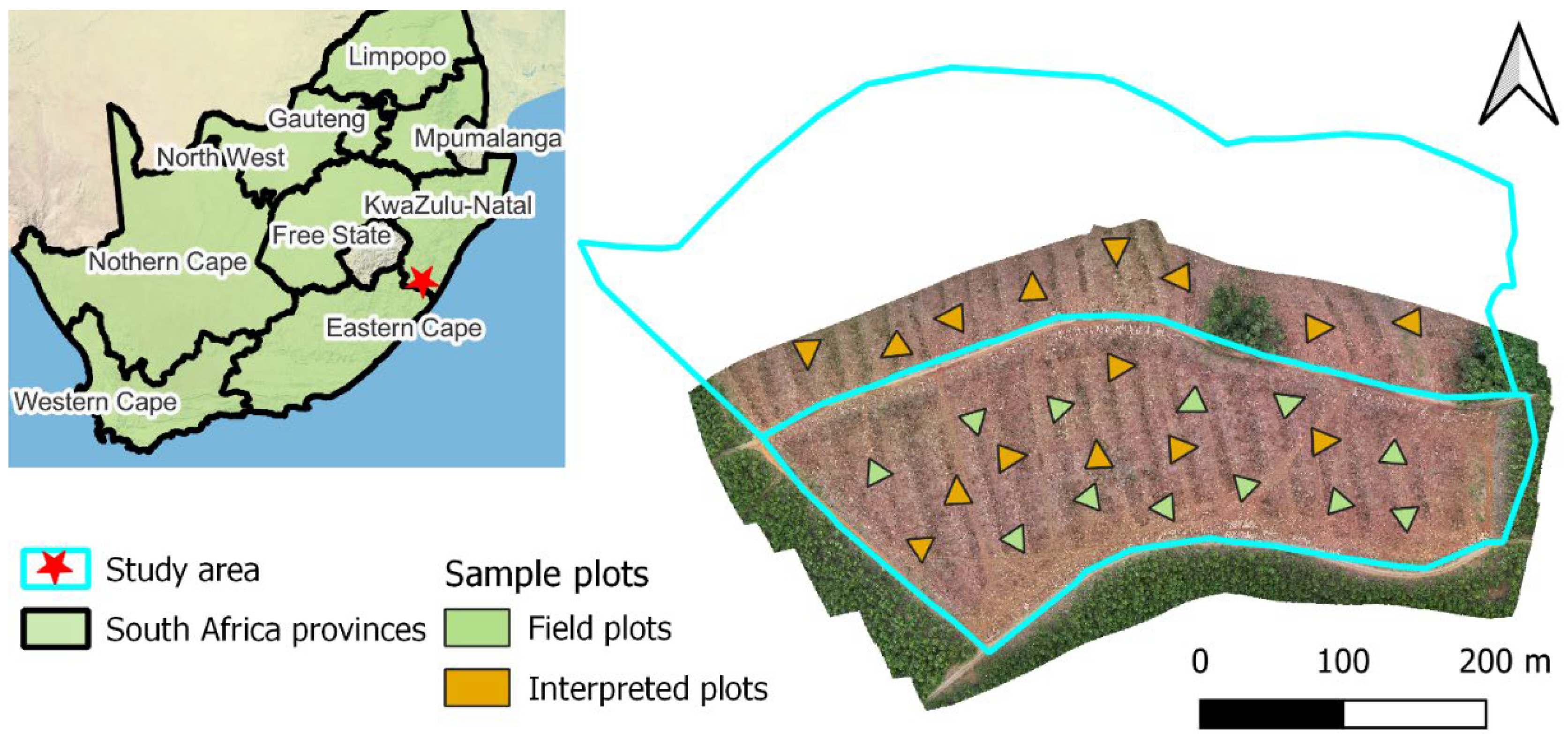
Figure 2.
(A) Example of a transect organization and localization with respect to a hypothetical machine trail, but could be applied generally; (B) Example of residues distribution over a plantation after a clear-cut; it is possible to notice the presence of material of different size.
Figure 2.
(A) Example of a transect organization and localization with respect to a hypothetical machine trail, but could be applied generally; (B) Example of residues distribution over a plantation after a clear-cut; it is possible to notice the presence of material of different size.
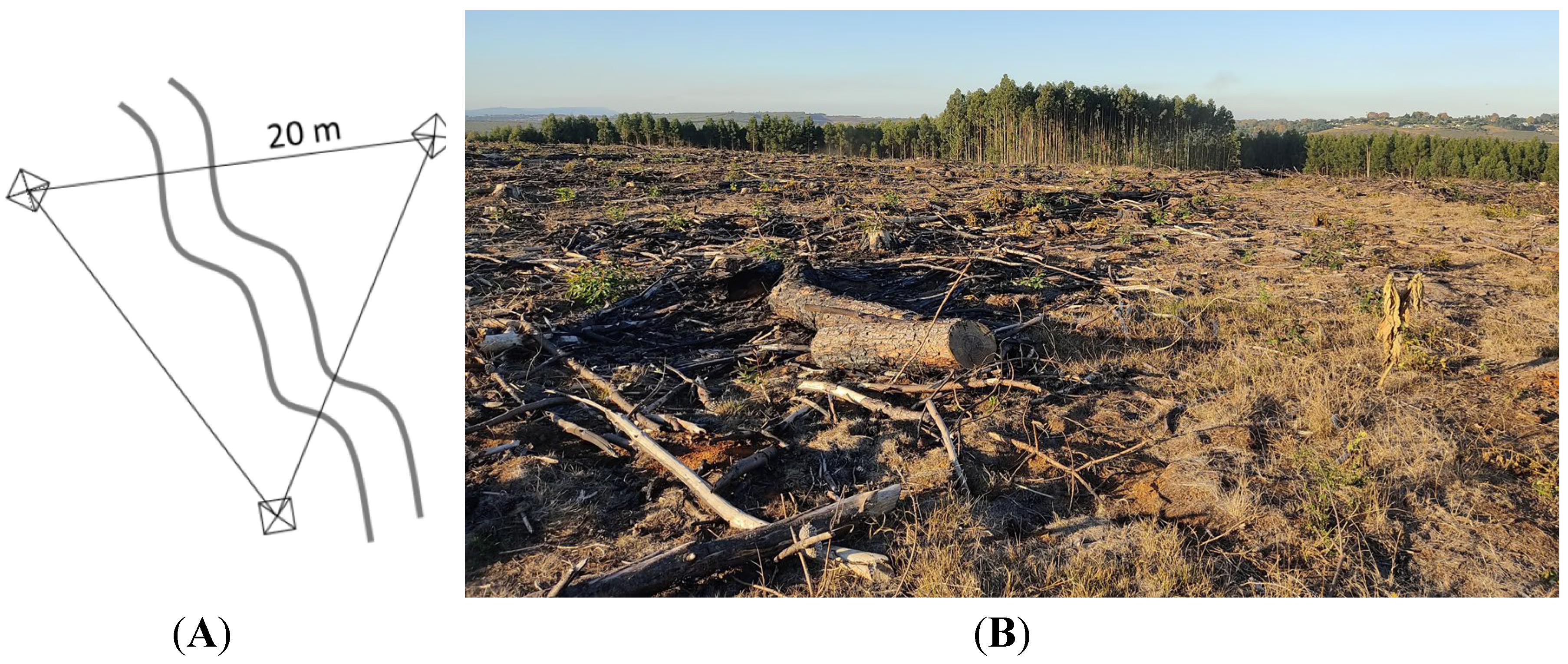
Figure 3.
Spatial and temporal distance (i.e., baseline) between the acquired images, also considering the subdivision into master and slave images.
Figure 3.
Spatial and temporal distance (i.e., baseline) between the acquired images, also considering the subdivision into master and slave images.
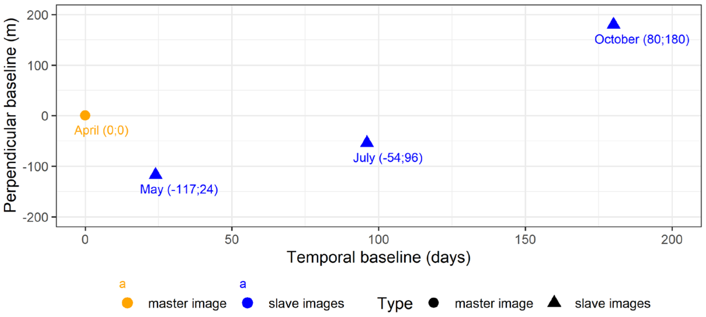
Figure 4.
Methodology flowchart to estimate residue mass using SAR and field data.
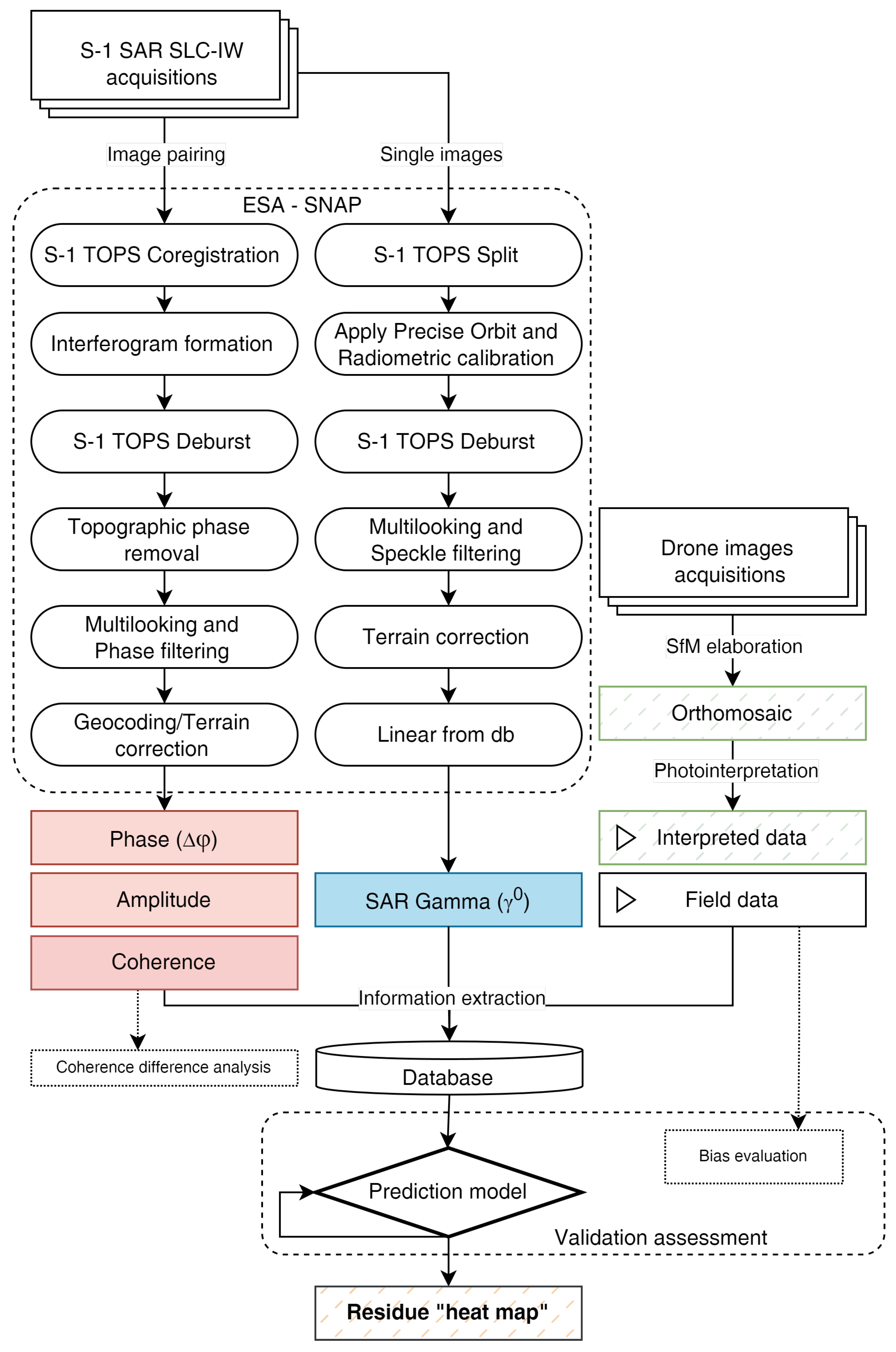
Figure 5.
The coherence difference obtained from and between the image pairs: A) April-May, B) April-July, C) Coherence difference between A and B, D) April-October, E) Coherence difference between A and D. The coherence scale in A, B and D is from 0–1, whereas the coherence difference scale is from -1 to 1.
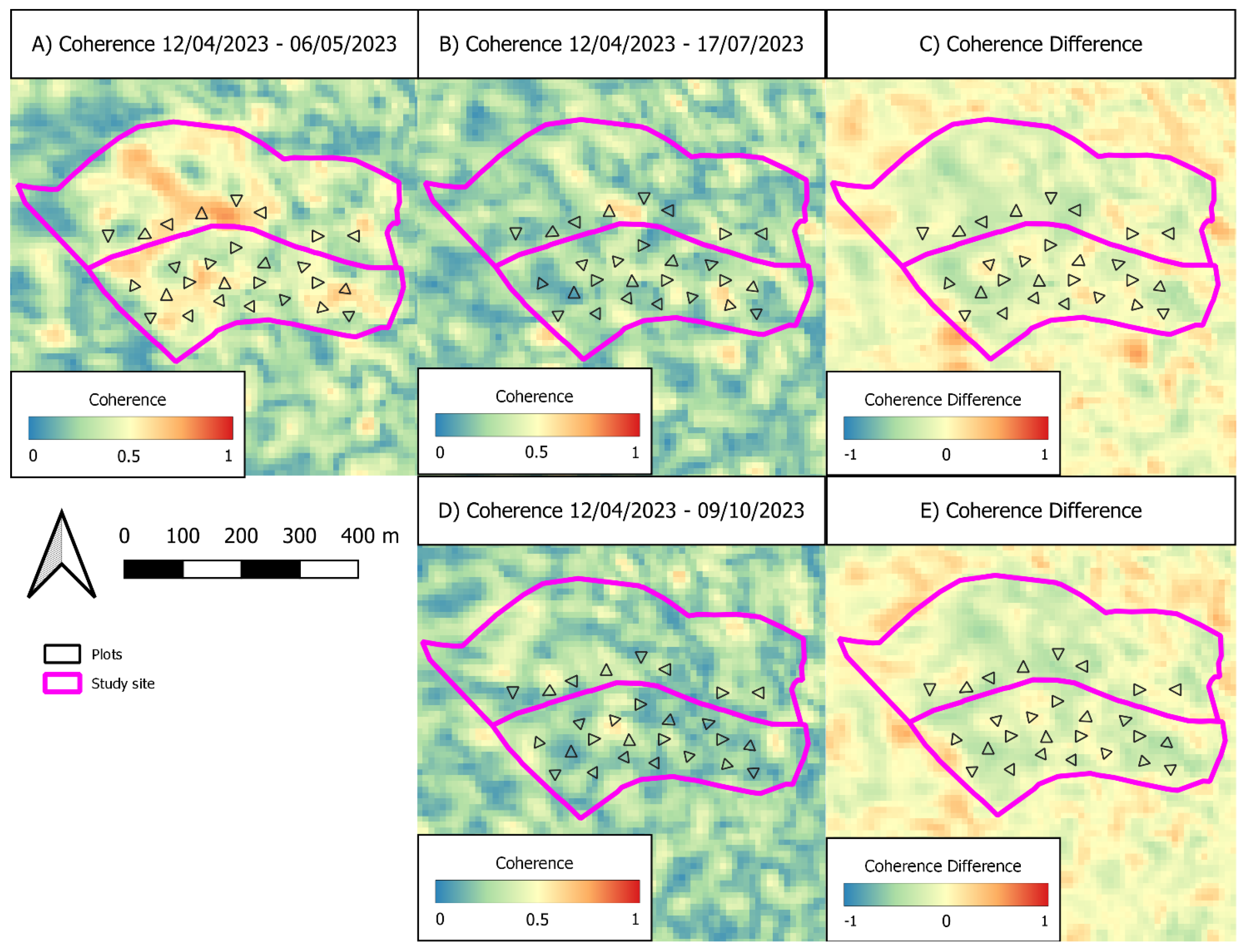
Figure 6.
Linear interpolation of predicted and field mass using Field plots (circles) and Interpreted plots (triangles) together for (A) GLM and (B) RF. The dashed line represents a 1:1 diagonal, whereas the full one depicts the regression line for the distribution.
Figure 6.
Linear interpolation of predicted and field mass using Field plots (circles) and Interpreted plots (triangles) together for (A) GLM and (B) RF. The dashed line represents a 1:1 diagonal, whereas the full one depicts the regression line for the distribution.
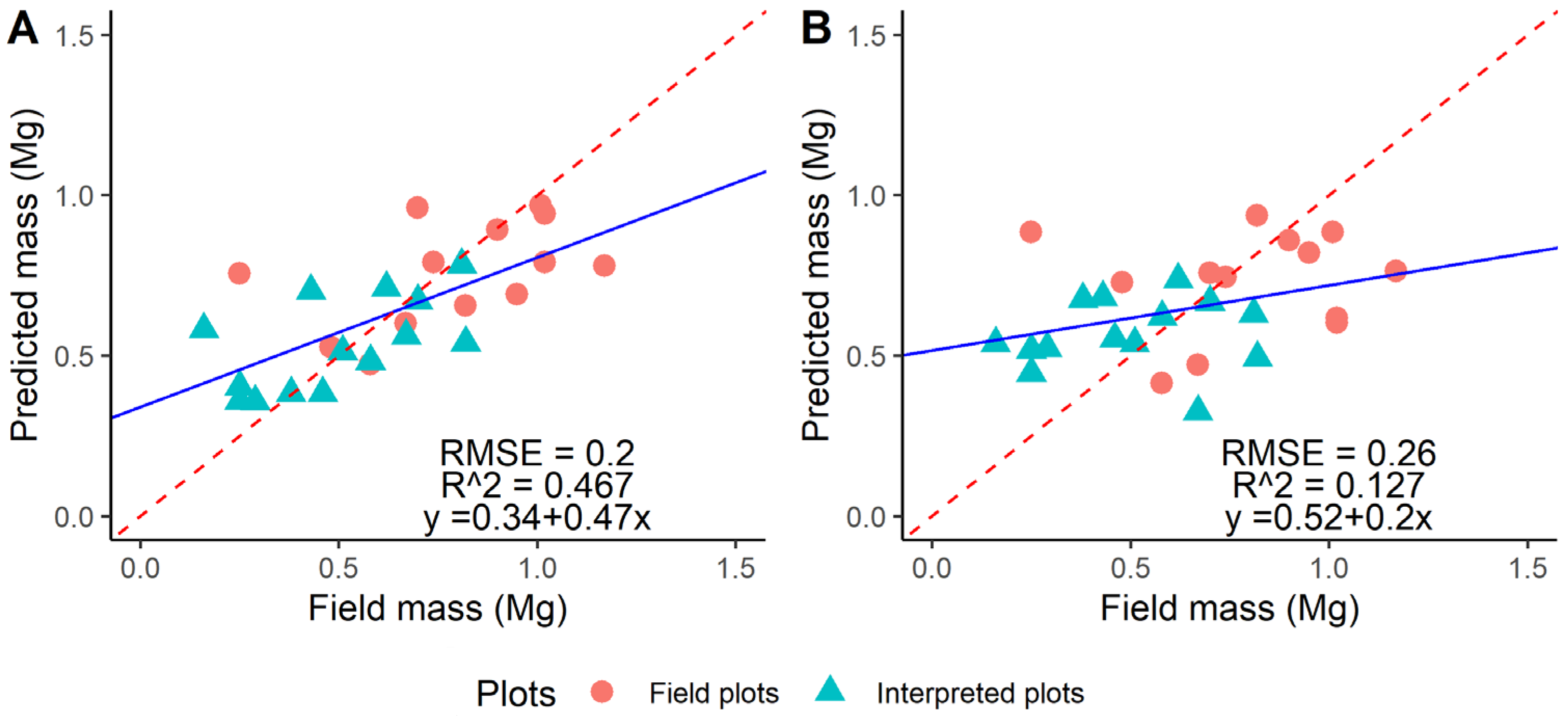
Figure 7.
Performance assessment through the linear interpolation of predicted and field mass for (A) GLM and (B) RF. The dashed line represents a 1:1 diagonal, whereas the full one depicts the regression line for the distribution.
Figure 7.
Performance assessment through the linear interpolation of predicted and field mass for (A) GLM and (B) RF. The dashed line represents a 1:1 diagonal, whereas the full one depicts the regression line for the distribution.
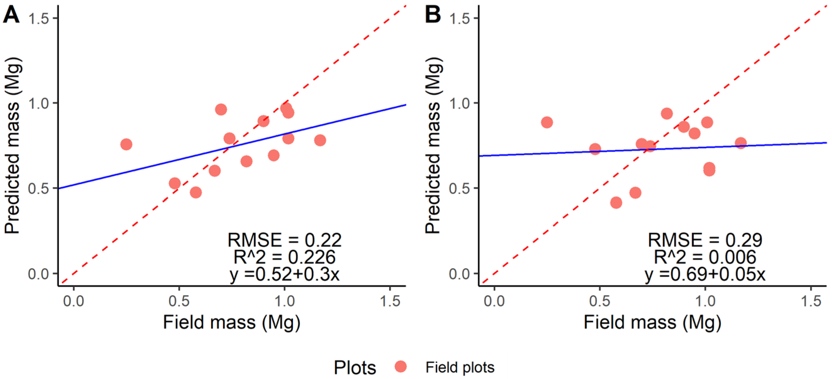
Figure 8.
The comparison of the predictions of the residue mass (i.e., residue “heat map”) performed by (A) GLM and (B) RF.
Figure 8.
The comparison of the predictions of the residue mass (i.e., residue “heat map”) performed by (A) GLM and (B) RF.
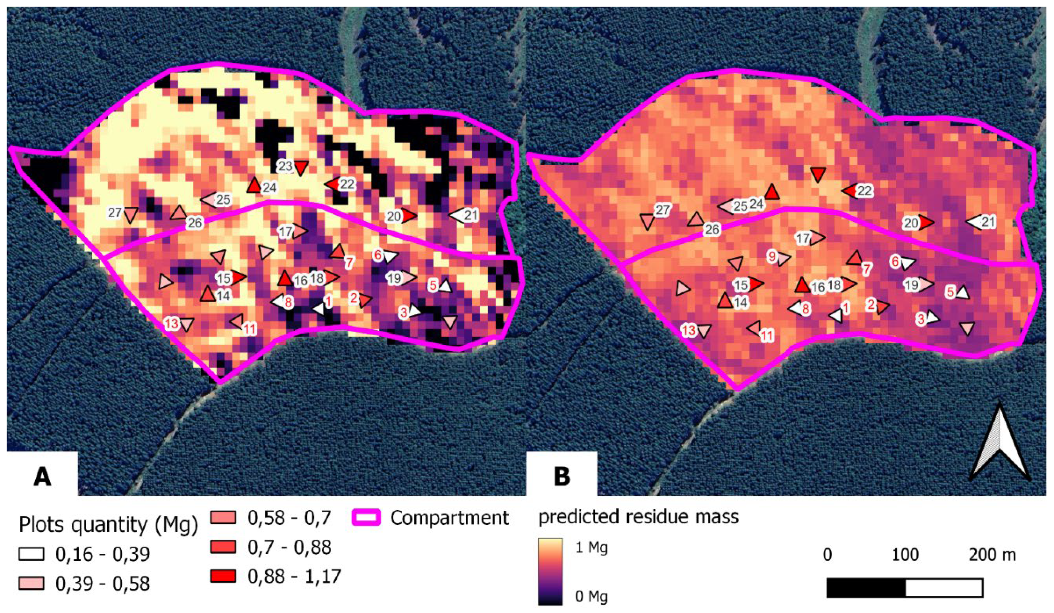
Table 1.
Average mass value (Mg ha-1) and actual mass value for residues (FWD - fine woody debris, CWD - coarse woody debris) for the study site and divided for each plot, also considering the division between field plots and interpreted plots. Standard deviation is also reported in brackets.
Table 1.
Average mass value (Mg ha-1) and actual mass value for residues (FWD - fine woody debris, CWD - coarse woody debris) for the study site and divided for each plot, also considering the division between field plots and interpreted plots. Standard deviation is also reported in brackets.
| Plot n. | Field Plots | Plot n. | Interpreted Plots | ||
|---|---|---|---|---|---|
| Mass estimator (Mg ha-1) | Measured Mass per plot (Mg) | Mass estimator (Mg ha-1) | Estimated Mass per plot (Mg) | ||
| 1 | 18.32 | 0.37 | 14 | 40.81 | 0.82 |
| 2 | 27.72 | 0.55 | 15 | 50.81 | 1.02 |
| 3 | 17.45 | 0.35 | 16 | 58.62 | 1.17 |
| 4 | 16.19 | 0.32 | 17 | 35.10 | 0.70 |
| 5 | 10.65 | 0.21 | 18 | 37.02 | 0.74 |
| 6 | 14.02 | 0.28 | 19 | 29.20 | 0.58 |
| 7 | 28.16 | 0.56 | 20 | 47.40 | 0.95 |
| 8 | 11.21 | 0.22 | 21 | 12.65 | 0.25 |
| 9 | 15.87 | 0.32 | 22 | 50.45 | 1.01 |
| 10 | 20.86 | 0.42 | 23 | 45.19 | 0.90 |
| 11 | 23.72 | 0.47 | 24 | 51.09 | 1.02 |
| 12 | 19.84 | 0.40 | 25 | 24.12 | 0.48 |
| 13 | 16.39 | 0.33 | 26 | 33.28 | 0.67 |
| - | - | 27 | 35.17 | 0.70 | |
| Average (St.dev) | 18.49 (5.30) | 0.37 (0.11) | 39.95 (11.92) | 0.79 (0.24) | |
Table 2.
Error assessment based on the field survey derived residue mass and the visual assessment residue mass over the field plots.
Table 2.
Error assessment based on the field survey derived residue mass and the visual assessment residue mass over the field plots.
| Error index | Unit | Value | |
|---|---|---|---|
| Average bias | CWD | Mg | -0.05 |
| RMSE | 0.20 | ||
| Average bias | FWD+CWD | Mg | 0.14 |
| RMSE | 0.20 |
Disclaimer/Publisher’s Note: The statements, opinions and data contained in all publications are solely those of the individual author(s) and contributor(s) and not of MDPI and/or the editor(s). MDPI and/or the editor(s) disclaim responsibility for any injury to people or property resulting from any ideas, methods, instructions or products referred to in the content. |
© 2024 by the authors. Licensee MDPI, Basel, Switzerland. This article is an open access article distributed under the terms and conditions of the Creative Commons Attribution (CC BY) license (http://creativecommons.org/licenses/by/4.0/).
Copyright: This open access article is published under a Creative Commons CC BY 4.0 license, which permit the free download, distribution, and reuse, provided that the author and preprint are cited in any reuse.


