Submitted:
14 August 2024
Posted:
14 August 2024
You are already at the latest version
Abstract
The relationship between the returns and volatility of stocks, gold, bonds, and Bitcoin (BTC) to changes in inflation, interest rates (SBI), and exchange rates is a compelling topic, encompassing factors such as inter-asset interactions, and the roles of assets as hedge or safe-haven. We aims the inter-assetscorrelation using Granger Causality Test and the role of hedge or safe-haven assets against uncertainty using GARCH for normal condition and quantile regression in crisis. Last, we built an optimal portfolio using the Arbitrage Pricing Model (APT) consists of 28% stocks, 16% gold, 27% bonds, and 29% BTC, with returns 1.7796% over the Rf. Monthly trading records from 2018 until 2023 are used. The results demonstrate a correlation between the returns of gold and bonds with BTC, while stock volatility is found to correlate with BTC volatility. Furthermore we found a negative correlation between gold returns and exchange rates, though gold shows no correlation with other variables, indicating its effectiveness as a hedge in normal conditions. The bond serve primarily as a diversifier against exchange rate and inflation in normal, bearish, and bullish market conditions. These findings suggest that gold and bonds are more stable instruments and serve as risk mitigation strategy for BTC.
Keywords:
Optimal Portfolio
; Safe-Haven Asset
; Hedge Asset
; Arbitrage Pricing Theory
; Bitcoin
; Gold
; Indonesia Stock Market
; Bond
; Inflation
; Exchange Rate
1. Introduction
The increasing global economic uncertainty is a result of various events, such as global inflation, the Ukraine-Russia war, and food shortages. The Indonesian government has implemented dynamic regulations, fiscal policies, and monetary policies to adapt to these changes. This situation can increase market information asymmetry and alter investor confidence, especially towards risky assets. During the Covid-19 pandemic, the stock market experienced a significant contraction, yielding a negative return of -0.008204 (Figure 1). Investors shifted from stocks to perceived safer assets like gold or bonds, known as flight-to-safety (Chen et al., 2023). The government gradually reduced interest rates from 5% to 4.5% in April 2020, and then to 4% in July 2020, to stimulate the market. This policy was positively received, resulting in positive returns from October to December 2020.
The volatility of the returns and prices of one asset will influence another asset (Köse et al., 2024). Figure 1 shows that bonds experienced negative returns of -0.007173 in July 2022 and -0.111115 in August 2022 due to the government’s decision to increase bond interest rates. This step was taken as a precautionary measure against rising inflation and the depreciation of the rupiah. In response, investors shifted to the stock market, which was seen as offering positive returns of 0.005720 in July 2022 and 0.032724 in August 2022. This aligns with the findings of Arshanapalli et al. (2006), who noted that the risk premiums of US bonds and stocks are positively correlated with conditional variances and covariances from 1979 to 2000, based on the CAPM method. They pointed out that bond and stock prices are interconnected and typically respond to announcements of labor, industrial, and Producer Price Index data. Consequently, investors experience negative abnormal returns when market sentiment is negative, and positive returns when sentiment is positive. Adrian et al. (2015) support these findings through their non-linear research using the polynomial VIX method on US Treasury Bonds from 1990 to 2007, showing that stock prices tend to increase with moderate to high volatility, while bond prices tend to decrease.
Between 2018 and 2023, gold prices consistently rose, achieving the second highest value in the past two centuries of global gold pricing history, peaking at $2,074 per ounce on August 6, 2020. Historically, gold has been viewed as an inflation hedge due to its weak positive or negative correlation with other assets (Arshad et al., 2023; Selmi et al., 2018). Previous studies have found that gold serves as a safe haven against monetary policy and the US dollar (Capie et al., 2005), helps maintain purchasing power during times of uncertainty, offers long-term advantages, and has high liquidity (Terraza et al., 2024). Gold is a homogeneous investment and a universally accepted medium of exchange. The return and price movements of gold consistently exhibit a positive trend in response to macroeconomic news and policy uncertainty (Selmi et al., 2018). However, Baur and Lucey (2010) suggest that long-term investment in gold is not advisable, especially during bull markets, due to the potential for opportunity costs.
In contrast, Bitcoin (BTC) experienced a significant price surge in March 2020 amid economic uncertainty caused by the virus outbreak. BTC investors enjoyed positive returns throughout 2020, except in June 2020 (-0.033781) and September 2020 (-0.074552). Selmi et al. (2018) noted that BTC attracts investors due to global uncertainties and diminishing trust in the banking system’s stability. BTC prices are highly dependent on market demand and supply dynamics. As a speculative asset, its limited supply makes BTC prices highly volatile, presenting considerable risks. BTC is deemed highly resilient during market disruptions and global uncertainties (Köse et al., 2024; Selmi et al., 2018), and its returns are unaffected by government or central bank policies (Paule-Vianez et al., 2020).
Portfolio formation involves several factors including: 1) asset valuation, 2) investment objectives, 3) asset allocation, and 4) diversification. Asset valuation and allocation involve the interrelationship between assets and the complexity of their interaction with macroeconomic changes to achieve the desired investor objectives. Asset diversification must consider the risks of each instrument and the correlations between assets. When uncertainty increases, investors will switch to other instruments that can avoid losses (Chen et al., 2023; Terraza et al., 2024). Understanding the relationships between assets helps investors choose non-correlated instruments to build portfolios that maintain or increase their value (Adrian et al., 2015). The role of hedge assets and safe-haven assets is needed to reduce losses and assist investors. This aligns with the prospect theory proposed by Kahneman & Tversky (1979) about investor irrationality, where investors tend to apply asymmetrical values to gains and losses by seeking a safe zone to avoid losses rather than pursuing equivalent gains, as their reference point is not total wealth.
Bottom of FormThis study aims to investigate the relationship between the returns and volatility of stocks, gold, bonds, and BTC concerning changes in inflation, interest rates, and the US dollar exchange rate. Following Paule-Vianez et al. (2020), we use price volatility and returns as dependent variables, while interest rates, inflation, and exchange rates are used as independent variables, and we conduct a Granger Causality test. Price volatility is estimated using Parkinson’s Volatility, which measures the difference between the highest and lowest values within the same period, while returns are calculated from the weighted average returns of the instruments. The goal is to understand the characteristics of each instrument and their interaction with the independent variables to form a better optimal portfolio.
The second objective is to determine which instruments can function as hedges or safe-havens under normal and uncertain conditions. We test the instruments under normal conditions using Generalized Autoregressive Conditional Heteroskedasticity (GARCH) to capture the heteroscedastic nature of asset volatility and returns (Maghrebi et al., 2006; Paule-Vianez et al., 2020). This method captures the volatility dynamics following changes in fiscal and monetary policy to determine portfolio investment strategies. We then build an optimal portfolio using the Arbitrage Pricing Model (APT), where returns are estimated based on their sensitivity to all systematic risks, as conducted by Amtiran et al. (2017) and Roll & Ross (1995). If investors know the magnitude of asset risk, they can measure the sensitivity of asset returns to that risk, and assets with similar risk sensitivity are close substitutes. The ability to select instruments and determine their composition is crucial for investors seeking to profit from their asset values in accordance with the risk they can bear. Finally, we analyze which instruments can function as hedges or safe-havens during a crisis. We use quantile regression to identify asymmetries that may not be visible in average regression as performed by GARCH under normal conditions. If macro conditions deteriorate, investors will seek these assets to reduce losses during crises, as seen in studies by Arshad et al. (2023), Paule-Vianez et al. (2020), and Selmi et al. (2018).
We acknowledge that many studies have explored the correlation between returns and economic uncertainty. However, we have not found the use of the APT method in accounting for increased idiosyncratic risk. APT assumes that the returns of financial assets are influenced by several macroeconomic factors as systematic factors, such as inflation rates, interest rates, and exchange rates. Although these risks cannot be avoided, investors can anticipate them if they know the magnitude and sensitivity of asset returns to these risks. We also take a novelty by forming an optimal portfolio consisting of four assets: stocks, gold, bonds, and bitcoin, which has not been studied before. The inclusion of BTC in the portfolio is generally avoided by risk-averse investors but is starting to be chosen by moderate and aggressive investors. This drives us to include BTC as part of asset diversification in the portfolio, despite the potential for high standard deviation values. The last novelty we offer is a discussion of the hedge and safe-haven roles of each instrument during a crisis. The increasing economic uncertainty has become a major concern for investors and governments worldwide, including Indonesia. Investors must be able to choose instruments that can keep their portfolio values stable or even reduce losses from their values.
This study is structured as follows: Section 2 presents a literature review supporting the relationship between instruments and economic uncertainty phenomena. Section 3 contains the data and methodology used. Section 4 explains the results and discussions built from the tests conducted. Section 5 provides the conclusions and implications of the research, while Section 6 offers opportunities for future research.
2. Literature Review
The Arbitrage Pricing Theory (APT), proposed by Roll & Ross (1995), asserts that asset prices are influenced by systematic risks that cannot be diversified away, and unsystematic risks that can be eliminated in a well-diversified portfolio. Systematic risks such as inflation (Amtiran et al., 2017; Tandiontong & Rusdin, 2015), bond yields, industrial production, and interest rate and market risks (Chen, Roll, and Ross, 1986; Miasary & Rachmawati, 2023) affect the risk sensitivity or beta of different sectors uniquely. Assets with similar risk sensitivities are close substitutes, distinguished by their unsystemic risks. Investors can use arbitrage strategies in their portfolios by leveraging market imbalances caused by systematic risks to generate profits. Over time, these arbitrage actions will establish a new market equilibrium, returning asset prices to their fair values.
Stock market volatility reflects the economy of a country, where the activity and presence of an integrated market indicate robust market conditions. Changes in monetary, fiscal, and government regulatory policies create uncertainty that is reflected in stock market trading. Conversely, changes made by the government or central bank will consider the market and its impact on stakeholders. This complex relationship is explained by various researchers, including Chen et al. (2023), who demonstrated that rising US inflation and increasing Fed interest rates lead to negative returns in the stock markets of G7 countries, except Japan. Amtiran et al. (2017) examined macroeconomic variables impacting Indonesia’s capital market and found that investors prefer domestic investments when the economy is stable, marked by falling interest rates, exchange rates, and inflation. When inflation rises, market returns decline, and the increased volatility in stocks heightens the risk, which can be offset by gold during periods of extreme negative returns (Baur & Lucey, 2010).
Since ancient times, gold has been regarded as a highly liquid investment, resistant to inflation, and a safeguard against losses. Baur and Lucey (2010) concluded that gold can preserve portfolio value because it typically has no or a negative average correlation with other assets (acting as hedge) during normal market conditions. They also found that gold serves as a safe-haven asset during volatile markets, due to its lack of or negative average correlation with other assets (Arshad et al., 2023). Hedge assets are characterized by their ability to reduce investor losses during extreme market conditions. This finding is supported by Baur and McDermott (2010), who studied the role of gold in G7 markets using daily, weekly, and monthly data with GARCH methods for normal times and quantile methods for crisis periods. Their results indicated that gold is a safe-haven during crises but not during normal times. Additionally, gold serves as a safe-haven against currency exchange rate fluctuations (Capie et al., 2005; Paule-Vianez et al., 2020). However, Aftab et al. (2019) found that gold primarily acts as a diversifier against exchange rate movements. This conclusion is reinforced by Köse et al. (2024), who used SVAR methods to analyze daily and weekly price data of gold, bitcoin, and the dollar. They found that gold has a significant positive correlation with exchange rates, indicating its role as a diversifier.
Bitcoin (BTC), often referred to as digital gold, has increasingly been seen as a safe-haven and hedge asset in recent years. Paule-Vianez et al. (2020) investigated the impact of economic policy uncertainty (EPU) on BTC by collecting EPU data from 2011 to 2019 and conducting quantile regressions with BTC volatility and return data over the same period. They concluded that BTC is a safe-haven asset during periods of high uncertainty, as shown by positive returns during crises. This conclusion is supported by Arshad et al. (2023), who exemined BTC behavior amid inflation in ASEAN countries and found its acts as a safe-haven in Indonesia and a hedge in other countries studied using the EGARCH method. The relationship between BTC and other investment instruments, such as energy and non-energy commodities, was examined by Bouri Elie et al. (2017). They concluded that BTC was a hedge before the 2013 European economic crisis and served as a diversifier afterward. Terraza et al. (2024) showed that the relationship between BTC, gold, and the US stock market has strengthened since the spread of Covid-19, with both BTC and gold acting as hedges against the stock market. Investors tend to exit the stock market when BTC returns increase and accumulate gold as another asset in their portfolios. This evolving understanding of gold and BTC underscores their significance as part of a diversified investment strategy, particularly during times of economic uncertainty and market volatility.
3. Data And Methodology
3.1. Data
This study relies on secondary data with time frame from January 1, 2018, to December 31, 2023. We use monthly transaction of stock trades, gold, Indonesian government 10-year bonds (http://www.investing.com), and Bitcoin (https://www.coindesk.com/price/BTC/), as dependent variables. These instruments are representing viable investment choices. Data on inflation, exchange rates, and Bank Indonesia interest rates (SBI) were obtained from the Indonesian Central Bureau of Statistics and Bank Indonesia websites. The risk-free rate used is the coupon rate of the Government Bonds SBR010. The variables used in this study are measured as shown in Table 1, following the methodologies of Arshad et al. (2023), Paule-Vianez et al. (2020), and Amtiran et al. (2017).
3.2. Analysis of Data
Our data analysis procedure begins by mapping all variables into a descriptive analysis to understand the type and distribution of the data. Especially for dependent variables, we, we forecast the dependent variable to determine the surprise factor. After it process we are conducting stationarity tests on all variables using the Augmented Dickey-Fuller (ADF) Test and the correlogram analysis to identify significant lags, autocorrelation patterns, seasonality, and cycles. The hypothesis is that if the p-value from these tests is below the significance level (< 0.05), the null hypothesis (Ho) is rejected, indicating that the data is stationary. Conversely, if the p-value exceeds 0.05, Ho is accepted, suggesting that the data is non-stationary, and differentiation is applied to achieve stationarity and remove unit roots.
Next, we investigate the causal relationships between assets using the Granger Causality Test, based on the study by Köse et al. (2024). The test employed to evaluate whether an uncertainty variable can be used to predict the dependent variable in a time series dataset over the monthly periods within the study’s timeframe. This method allows us to evaluate the predictive influence of economic uncertainty on asset returns and their interactions over time.
If is the dependent variable, then is the model constant. The variable represents the predictive variable tested against . The influence of the lagged Y at t-i is indicated by the coefficient and is the influence of the lagged X at t-j. If ≠ 0, then X has predictive power over Y, and vice versa.
Once the relationship is mapped, we forecast the variables Exc, Inf, and SBI using the simple exponential smoothing method to identify the surprise factor values from systematic risk (Miasary & Rachmawati, 2023). This method predicts future values based on the repetition of past patterns by smoothing out irregular components of the data through weighted averages of past observations. The advantage of this method is that it uses data without trends or seasonality and assigns decreasing weights to longer-term observations, making it more responsive to the uncertainties of systematic risk. The formula used is:
After mapping the relationships, we forecast the variables Exc, Inf, and SBI using the simple exponential smoothing method to identify the surprise factors from systematic risk (Miasary & Rachmawati, 2023). This method predicts future values based on past patterns by smoothing out irregular data components through weighted averages of past observations. The benefit of this method is more responsive to systematic risk uncertainties and it applies to data without trends or seasonality and assigns decreasing weights to older observations. The formula we used:
where represents the prediction for the upcoming period while is the current forecast derived from the previous period and is the actual value in the current period. After determining the forecasts for each systematic risk, we evaluate asset prices using the Arbitrage Pricing Theory (APT). Under APT, the expected return is calculated based on several systematic risks or factors exert a linear influence on the market under equilibrium conditions. The sensitivity of an asset’s return to changes in systematic risks is analyzed using time series and cross-sectional data, as illustrated by the formula below:
where represents the sensitivity of instrument i to factor k dan refers to the surprise factors. These values are calculated as the actual values minus the predicted values. However, this factorial model does not yet describe the equilibrium condition of the model, necessitating a cross-sectional regression between the expected return and the systematic risk of each factor for the investment instruments. The risk premium of the instrument ( and are obtained from the expected return of the instruments and factor k minus the risk-free rate (Rf). To analysis data, we implemet univariate GARCH regression accros all variables to estimate volatility overtime, serving as risk mitigation and price derivatives strategy (Arshad et al., 2023; Baur & Lucey, 2010; Köse et al., 2024). The GARCH (0,1) model we employ follows the formula:
If is dependent variable at t period then represents model’s constant and is shock at time t, the formula given by . The conditional variance at time t is defined as where , and are the model parameters. Here is the squared shock from time t-1 and is conditional variance at time t-1. These estimated result are used to detect the hedging role of each instrument under normal conditions. The hypothesis posits that an asset serves as a hedge if the p-value in the GARCH model is below the significant levela (< 0.05) a nd the variable’s coefficient is negative. Conversely, an asset functions as a diversifier if the p-value is below the significance level (< 0.05) but the coefficient is positive.
The next step involves constructing an arbitrage portfolio based on several key assumption 1) The investors will not inject additional capital into the portfolio, denoted by , where is the weight of each instrument into portfolio, 2) the arbitrage portfolio should have no sensitivity to systematic risk factors, expressed by where is weighted average sensitivity of assets within portfolio and 3) The portfolio is structured to yield positive expected returns, mathematically validated by , where is expected return.
We recognize that the study period encompassed the Covid-19 pandemic from 2020 to 2022, which led to increased volatility and uncertainty in market instrument prices. The GARCH method, however, has limitations due to its volatility persistence and inability to capture asymmetries, unlike the EGARCH and TARCH models. To address these limitations, we supplemented our analysis with quantile regression, following the approaches of Arshad et al. (2023), Paule-Vianez et al. (2020), and Selmi et al. (2018). This method serves as a valuable benchmark for investors aiming to construct more resilient and stable portfolios during financial crises. We use quantiles of 0.06 and 0.07 to identify asymmetry during bearish period and quantiles of 0.8 and 0.9 during bullish one. If the quantile regression results indicate a significant negative β coefficient or no correlation, we can conclude that the asset acts as a safe haven (Baur & Lucey, 2010; Bouri Elie et al., 2017). In such cases, investors will pursue these assets to mitigate losses during economic crises. Conversely, if the p-value is below the significance level (< 0.05) but the coefficient is positive, the asset serves as a diversifier.
4. Empirical Results and Discussion
4.1. Descriptive Analysis of Data
We conducted a descriptive analysis of the returns and price volatility for all instruments as detailed in Table 2, highlighting several key points. Notably, BTC is a highly speculative asset with significant volatility, exhibiting a substantial disparity between its maximum and minimum values. Its average return is the highest at 0.04109, which correlates with the highest volatility of 0.30714. This finding supports the research by Köse et al. (2024), Selmi et al. (2018), and Terraza et al. (2024), which suggest that bitcoin is a speculative asset. Bonds provided an average return of 0.00124 with the lowest average volatility of 0.05868 among the instruments, supporting Arshanapalli et al. (2006), who noted an inverse relationship between bond volatility and returns. Stocks offer an average return of 0.007434 with an average volatility of 0.06447, which is the second highest among all instruments. Adrian et al. (2015) noted that increased stock volatility leads investors to expect higher returns, whereas bond returns decrease as investors are compensated with higher coupon rates. During periods of high stock volatility, investors tend to favor bonds over stocks (flight-to-safety). Gold provides an average return of 0.00678, the second highest after bitcoin, with an average volatility of 0.06473. The data distribution shows that market returns are not normally distributed, with a left-skewed tail, while volatility is right-skewed with leptokurtic kurtosis. In contrast, the return distributions for gold and bitcoin are approximately normal, with right-skewed skewness and leptokurtic volatility distributions for both. Bond returns exhibit a non-normal distribution with leptokurtic skewness and kurtosis. These conditions indicate the presence of outliers in both return and volatility data. We will detect these outliers using the Mahalanobis method and replace the outlier values with the mean values.
We also assess Inf, Exc and SBI as indicators of economic uncertainty, detailed in Table 3 below. Throughout the observation period, the rupiah exchange rate experienced a significant negative contraction in May 2020, resulting in a minimum return of -0.02925. However, on average, the exchange rate returns remained positive at 0.00354, due to Indonesia’s managed floating exchange rate system. The currency price mechanism is determined by the market, but the Central Bank can use monetary policy to stabilize prices through triple intervention, including interventions in the spot market, Domestic Non-Deliverable Forward (DNDF) market, and government securities buybacks. Fisher’s theory states that investors tend to demand higher interest rates as compensation for rising inflation and the loss of expected market returns. Reflecting this, the government adjusted its monetary policy after the COVID-19 pandemic to counteract rising inflation, global supply chain issues, and soaring energy prices. Notably, Bank Indonesia increased the SBI rate in September 2022 from 3.50% (June 2022) to 4.75%. As of April 2024, the BI 7-Day Reverse Repo Rate (BI7DRR) has reached 6.25%, with data indicating an average positive SBI return of 0.00389. Indonesia’s average inflation rate stands at -0.00304, suggesting that stringent monetary policies have effectively lowered the prices of essential goods and services. The distribution statistics in Table 3 indicate that the exchange rate and inflation data are normally distributed, while the SBI data is leptokurtic, with a value of 15.01046.
Next, we determined the surprise values for the factors Exc, Inf, and SBI using the exponential smoothing method in Eviews 13. This method is particularly effective for short-term forecasting, which aligns with our analysis. The results are displayed in Figure 2 below.
4.2. Correlation Between Instruments
After all the surprise factors and other variables were structured, we conducted a stationarity test using the ADF Test to ensure that the data exhibited constant variance and mean, which enhances the stability and validity of the predictive model. According to the results in Table 4, all variables except SBI had a probability value of 0.0000, indicating that the null hypothesis was rejected and the data were stationary at the level. For the SBI variable, we applied first differencing, and the results showed that the probability value at this level was below the significance threshold.
We performed Granger Causality tests on all instrument returns using a lag length of 3. The results, presented in Table 5 below, revealed only two short-term causal relationships: one between gold returns and BTC returns, and the other between bond returns and BTC returns. The return on gold or the return on 10-year government bonds of Indonesia influences the return on BTC, but not vice versa. This relationship suggests that gold and government bonds can serve as risk mitigation tools for BTC investors. These results corroborate the findings of Arshad et al. (2023), Baur & Lucey (2010), and Terraza et al. (2024), who discussed the connection between gold and BTC. But contrast from those of Chen et al. (2023), who explored the flight-to-safety phenomenon from high-risk to low-risk assets. The lack of a relationship between stock market returns and the returns on gold, government bonds, and BTC indicates that these instruments move independently without influencing each other under normal market conditions (Baur & McDermott, 2009). The Granger test also shows that stock price volatility affects BTC price volatility but not vice versa. These findings align with Arshad et al. (2023) but contradict Bouri Elie et al. (2017), who stated that BTC has a negative correlation with energy commodity stock markets and a positive correlation with non-energy commodities. We conclude that a decline in stock prices leads aggressive investors to turn to BTC, which exhibits highly fluctuating price movements.
4.3. Hedge Acts in Normal Condition
The subsequent phase involves verifying the hedging capabilities of the four instruments against economic uncertainty using the GARCH (0,1) model, as depicted in Table 6 below. It was observed that Rm exhibit a significant negative correlation with Exc (βExc = -1.1436), while Vm have a significant positive correlation with Exc (βExc = 0.6521). This relationship highlights the integration between the domestic currency market and the stock market. Exchange rates are critical indicators for investors because it can change in a very short period compared to other variables. We conclude that stock returns serve as a hedge under normal market conditions, while their price volatility acts as a safe haven against the same variable. These findings are consistent with the studies by Amtiran et al. (2017), Chinzara (2011), and Maghrebi et al. (2006), though it contradict the results of Köse et al. (2024). Furthermore, the regression results reveal a significant negative correlation between Rm and Inf (βInf = -0.0585), supporting the conclusions of Chen et al. (2023) and Maghrebi et al. (2006). When inflation decreases, stock price volatility increases, driven by investors’ desire for gains from risky assets.
From Table 6 above, Rg exhibits a significant negative correlation with Exc (βExc = -1.3825), while Vg shows a significant positive correlation with Exc (βExc = 0.2296). This indicates that gold returns hedge against exchange rate fluctuations but not against Inf or SBI. Gold helps protect an investor’s portfolio value during currency depreciation. From a volatility perspective, we observe that the appreciation of the rupiah is in line with global gold prices. It indicates that suggesting gold’s role as a diversifier. When gold prices rise and the rupiah appreciates, investors will buy gold, driving its price even higher. This finding aligns with the traditional Indonesian perception of gold as a highly liquid and safe investment, symbolizing wealth and passed down through generations. This cultural perception influences conservative investors to prefer gold. Our results support those of Paule-Vianez et al. (2020), Baur & Lucey (2010), and Baur & McDermott (2009), identifying gold as a hedge, and align with Aftab et al. (2019) and Köse et al. (2024), who recognize gold as a diversifier.
We also demonstrate that 10-year government bonds are diversifiers that can help investors reduce losses during global uncertainty. The analyzing of relationshif of Rb against Exc and Inf reveals significant positive correlations at 1.1910 and 0.0996, while Vb has a significant positive correlation with the Exc at 0.5453. This contrasts with Chen et al. (2023), who reported that US inflation negatively impacts G7 country bond prices across various maturities, suggesting bonds can serve as a hedge. This difference is due to the spillover effects of US stock market volatility and monetary policy on the global economy.
Finally, we find that Rbtc is solely influenced by the Exc at -2.7089 and is unaffected by other variables. The negative correlation suggests BTC’s role as a hedge during rupiah depreciation, supported by positive returns throughout the study period. Vbtc is unaffected by all dependent variables, consistent with Bouri Elie et al. (2017) and Terraza et al. (2024). This supports previous findings that BTC is resistant to inflation (Arshad et al., 2023) and immune to government monetary policies (Paule-Vianez et al., 2020). We concur with Selmi et al. (2018) that BTC returns are driven by supply and demand dynamics and market availability. However, BTC returns are influenced by both positive and negative news, especially fraud and hacking incidents, which can generate negative sentiment (Köse et al., 2024).
The findings in Table 6 above demonstrate that GARCH (0,1) is significant across all tests, as evidenced by the probability values below the significance threshold. However, the GARCH coefficient is not significant. The value of C in the variance equation refers to the conditional variance at time t being influenced by the conditional variance at the previous period (t − 1). This suggests an autoregressive impact on the current return volatility and price volatility of each instrument for the next period’s return volatility and price volatility. Additionally, the GARCH return variance reveals significant persistence in volatility, which tends to remain over time. All models were tested for heteroskedasticity using the ARCH-LM test, confirming the absence of heteroskedasticity with Prob. F values greater than the 0.05 significance level. The low AIC values in all tests suggest that the model has a good fit for predicting the relationship between return volatility and the movement of all instruments.
4.4. Safe-Haven Acts in Crisises Condition
Next, we conducted quantile regression in Table 7 above to analyze the behavior of return volatility and prices under bearish at the percentiles of 0.06 and 0.07, and bullish condition at 0.8 and 0.9.
We revealed a significant negative relationship between Exc and Inf on Rm, indicating that the stock market can function as a safe-haven during bearish phases. Nevertheless, Rm serves primarily as a diversifier in bullish periods, indicated by a significant positive coefficient to Inf. This finding supports Chinzara’s (2011) conclusion on the interconnection between money and stock markets in emerging economies. During currency depreciation and high inflation, investors receive positive returns as compensation for portfolio losses. These positive returns indicate that companies are performing well, aimed at maintaining future cash flows through efficiency and improved performance.
Conversely, during bearish phases, none of the independent variables significantly impact Vm. Our result contradicts Chen et al. (2023) regarding flight-to-safety but it demonstrates investor trust in the government’s ability to maintain macroeconomic stability, particularly in stabilizing the exchange rate and controlling inflation. We concur with Maghrebi et al. (2006), who noted that the political regime in Asian countries influences market volatility when confronted with currency depreciation. Our findings are also consistent with parts of Köse et al. (2024), which stated that stock price volatility is unaffected by exchange rates, inflation, or interest rates during crises. Nevertheless, we found that Vm has a positive relationship with interest rates during bullish periods, similar to the conclusions of Amtiran et al. (2017), further supporting our conclusion that there is no flight-to-safety from the stock market to low-risk assets during both bullish and bearish.
Gold continues to be a safe-haven investment during crises driven by currency depreciation in Indonesia, as evidenced by a significant negative correlation between Rg and Exc. This result aligns with Capie et al. (2005) and Paule-Vianez et al. (2020). However, during crises triggered by inflation and interest rates, gold serves as a diversifier, marked by a significant positive correlation. We also observed a similar role during bullish periods, indicating that Rg only act as a diversification asset against Exc and Inf. This outcome is in line with Baur & McDermott (2010), Aftab et al. (2019), and Arshad et al. (2023), who who stated that gold does not act as a safe-haven or hedge during normal periods or post-crisis.
An interesting observation we made is Rb only act as diversifiers for Exc under bearish and bullish conditions, although this role is not evident at the extreme quantile of 0.06. Similarly, Vb can only act as a diversification asset for Exc and Inf during bullish phases, this result contradicts Chen et al. (2023). We suspect that there are several reasons for this low volatility in the face of uncertainty, including: 1) the Fed’s interest rate hikes from 2020 to 2022 were more attractive to investors compared to Indonesia’s 10-year government bond yields, and 2) the increase in Indonesian government debt from 4.917 quadrillion rupiahs in 2018 to 8.002 quadrillion rupiahs is an unfavorable sentiment for investors. This conclusion aligns with Mita Niia & Hamzah (2021), who found that investors preferred not to invest in long-term Indonesian government bonds post-economic recovery following the discovery of the Covid-19 vaccine due to the government’s debt burden.
Rbtc act as a safe haven against Inf during bearish periods, marked by a significant negative correlation in 0.06 and 0.07 percentile while Rbtc serves as a safe haven against SBI in bullish periods,. These results are consistent with the findings of Bouri Elie et al. (2017), Köse et al. (2024), Paule-Vianez et al. (2020), and Terraza et al. (2024). We conclude that BTC’s high price volatility during crises precludes its use as a currency. However, this volatility can make BTC a profitable investment for investors with a high tolerance for risk. Top of Form
4.5. Optimal Portfolio
Finally, we conducted a cross-sectional test to validate the factor loadings in this study using panel data regression on ARMA (3,0). The results show that Er is influenced by changes in Exc and Inf but not by SBI in Table 8 below. This suggests that investors have successfully anticipated changes in interest rates to mitigate their portfolio risks. Conversely, the government’s ability to stabilize exchange rates and control inflation is a more critical indicator for investors. The R-Squared value of the test is 0.2385, indicating that the independent variables can only explain 23.85% of the dependent variable, with the rest attributed to other factors. The standard deviation of the model is 0.9751, indicating that the model is reasonably accurate.
The purpose of all analyses is to identify the correlation between assets and their relationship with systematic risk. Using the factors that constitute the portfolio, we determine asset allocation using the APT method by forming an arbitrage portfolio based on expected returns and factor loadings analyzed with time series and cross-sectional data under normal conditions (Table 9).
We assume that the weight of Rm ( is 0.03 and calculated the weights of each instrument using python. The computed weights are = 0.0176 dan = 0.0396. Subsequently, we multiplied the weights of each instrument by their expected returns to calculate the expected return of the arbitrage portfolio. The result is 0.00132 or 0.132%, indicating that the arbitrage portfolio has been successfully identified. Investors will continue to engage in arbitrage in the market until a new equilibrium price is reached. Therefore, we constructed an optimal portfolio under the assumption that investors have evenly allocated their funds across the four instruments in the portfolio, as shown below:
According to Table 10, the negative allocation of gold in the arbitrage portfolio suggests that investors can short sell gold and shift to other assets to maintain their wealth. The optimal portfolio is composed of 28% stocks, 16% gold, 27% bonds, and 29% BTC. The expected return for this optimal portfolio is calculated by multiplying the weights of the instruments by their expected returns, resulting in 0.017796 or 1.7796%, which exceeds the risk-free rate. The portfolio’s risk is a linear function of the loading factor and the risk-free rate return, formulated as follows:
From model above, we can assume if all the loading factors are 0 then the investor would expect a return of 0.00596, equivalent to risk-free rate. However, if the rupiah depreciates by 1%, the portfolio return would increase by 0.2402. Conversely, if inflation risk decreases by 1%, the portfolio return would increase by 0.1901.
5. Conclusion and Implementation
Over the past decade, significant global economic changes have increased the volatility of returns and prices of market instruments. To navigate the condition, investors must formulate effective investment strategies by considering the relationships between instruments and their exposure to systematic risks. Initially, it is essential to examine the correlations between assets to comprehend their movements, thereby enabling effective portfolio diversification. A positive or negative correlation indicate that the returns and prices of one instrument are influenced by another. Investors can strategically buy inversely correlated assets and short-sell positively correlated ones. Further, investors need to evaluate the correlations between instruments and systematic risks to identify assets that can function as hedges or safe-havens under varying conditions. Hedge assets can preserve portfolio value during normal conditions due to their inverse correlation, while safe-haven assets can enhance portfolio value during times of uncertainty.
Using the Granger Causality Test, we investigated the correlation of returns and prices among stocks, gold, 10-year government bonds, and bitcoin. Our findings reveal that g the returns of gold and bonds are correlated with BTC returns, while stock volatility is correlated with BTC price volatility. We concluded that gold and 10-year government bonds are more stable instruments and serve as risk mitigation measures for BTC investors in Indonesia. Meanwhile, stock price volatility can be used as an asset diversification strategy in BTC portfolio. Given BTC’s speculative nature and significant price volatility, poses risks to portfolio value, especially for conservative investors. Thus, mitigating and diversifying strategies using gold, bonds, and stocks are the best approaches under normal market conditions.
Additionally, we investigated the relationship between instruments and systematic risks such as exchange rates, inflation, and interest rates using the GARCH (0,1) method under normal conditions and quantile regression under uncertainty. Our findings suggest that stock returns serve as hedges and diversifiers against exchange rate and inflation changes in normal markets. In bearish phases, stocks act as safe-havens, whereas in bullish phases, they function as diversifiers. Exchange rates are critical indicators frequently observed by investors due to their rapid fluctuations over short periods compared to other variables. We acknowledge that Indonesia’s extensive international trade, primarily conducted in US dollars, means currency depreciation boosts export competitiveness and company profitability, thus driving up stock prices and returns, particularly in industries like palm oil, coal, rubber, and gas. Maghrebi et al. (2006) state that depreciation impacts more significantly than appreciation in similar events. The close relationship between the domestic stock market and the currency market can be a good indicator for investors before taking buy or sell positions in the stock market.
We identified a significant negative relationship between gold returns and exchange rates, though no significant ties were found with other variables. This suggests that gold serves as an effective hedge against exchange rate volatility under normal circumstances. Conversely, the volatility of gold prices acts as a diversifier against exchange rate fluctuations, indicating that currency depreciation can be mitigated through gold purchases to sustain or boost portfolio value. In crisis periods, gold functions both as a safe-haven and a diversifier against all three systematic risks. Public perception of gold as a universally accepted currency with high liquidity has elevated its returns and prices amidst currency depreciation, inflation, and interest rate variations. This finding aligns with the traditional Indonesian perception of gold as a highly liquid and safe investment, symbolizing wealth and passed down through generations. This cultural perception influences conservative investors to prefer gold.
Furthermore, our findings show that returns on 10-year government bonds only act as diversifiers against exchange rate and inflation changes due to their significant positive relationship across normal, bearish, and bullish markets. Bond price volatility also diversifies against exchange rate changes in normal and bullish markets and against interest rate changes during bullish phases. These results contrast with Chen et al. (2023) but support Mita Niia & Hamzah (2021), who state that the government compensates for higher debt ratios and bond risks by offering increased returns. Investors can take advantage of this by investing in short- to medium-term bonds, but preferred not to invest in long-term Indonesian government bonds post-economic recovery following the discovery of the Covid-19 vaccine due to the government’s debt burden.
We also found that BTC returns are significantly negatively affected by exchange rates, while its price volatility is unaffected by the three independent variables under normal conditions. During bearish markets, BTC can act as a safe-haven against inflation, and during bullish periods, it serves as a safe-haven against changes in Bank Indonesia’s interest rates. We conclude that BTC is resistant to inflation and monetary policy but is susceptible to news sentiment, particularly regarding fraud and hacking. BTC’s lack of underlying assets and high price volatility can be concerning for conservative investors, yet it remains attractive to those with higher risk tolerance. We advise BTC investors to diversify their portfolios with more stable instruments and serve as risk mitigation such as gold and bond to preserve their wealth, especially during crises.
Return and risk are key factors in investor decisions. Investors aim to maximize returns while minimizing risk. The APT method is a multi-factor asset valuation method that can be used to form an arbitrage portfolio based on expected returns and factor loadings analyzed using time series and cross-sectional data. Our research indicates that the optimal portfolio composition consists of 28% stocks, 16% gold, 27% bonds, and 29% BTC, with returns exceeding the risk-free rate at 1.7796%. However, arbitrage conditions will be followed by other investors, causing asset prices to reach a new equilibrium, and investors must re-estimate their portfolio composition by considering macro factors and global economic conditions. Our optimal portfolio can be effectively utilized by investors if the government maintains a managed floating exchange rate system, allowing the central bank to intervene and stabilize the rupiah, thereby encouraging stock market investment.
Our formatting portfolio require investor to avoid re-injection fund and determine tolerance risk limit that investors are willing to bear. It is better to reduce weight of high risk instrument for conservatif investors while moderat and aggressive investors can assign stoploss and profit target to be achieved in our portfolio model.
6. Future Research
The formation of a portfolio comprising four instruments is a spectacular and daring endeavor. The allocation of each instrument is determined by the price trends and returns of the assets over the past six years. We acknowledge that during this period, the spread of the virus caused the world to nearly come to a standstill, impacting economic recovery to this day. This situation led to highly fluctuating asset returns and prices, which serves as a disclaimer for very risk-averse investors. We recommend incorporating investor classification as a risk factor that can be used in subsequent research to ensure that the formed portfolio aligns with the risk tolerance levels. Additionally, the APT method is a multi-factor model where return volatility can be influenced by various systemic factors. We acknowledge that using three risk variables, namely exchange rate, inflation, and interest rates, only explains 23.85% of the return-forming factors. We open the possibility for further research by including other systemic variables so that the factors influencing return volatility can be more elaborated.
References
- Adrian, T., Crump, R. K., & Vogt, E. (2015). Nonlinearity and Flight to Safety in the Risk-Return Trade-Off for Stocks and Bonds. SSRN Electronic Journal, November. [CrossRef]
- Aftab, M., Shah, S. Z. A., & Ismail, I. (2019). Does Gold Act as a Hedge or a Safe Haven against Equity and Currency in Asia? Global Business Review, 20(1), 105–118. [CrossRef]
- Amtiran, P. Y., Indiastuti, R., Nidar, S. R., & Masyita, D. (2017). Macroeconomic factors and stock returns in APT framework. International Journal of Economics and Management, 11(SpecialIssue1), 197–206.
- Arshad, S., Vu, T. H. N., Warn, T. S., & Ying, L. M. (2023). The Hedging Ability of Gold, Silver and Bitcoin Against Inflation in Asean Countries. Asian Academy of Management Journal of Accounting and Finance, 19(1), 121–153. [CrossRef]
- Arshanapalli, B., d’Ouville, E., Fabozzi, F., & Switzer, L. (2006). Macroeconomic news effects on conditional volatilities in the bond and stock markets. Applied Financial Economics, 16(5), 377–384. [CrossRef]
- Baur, D. G., & Lucey, B. M. (2010). Is gold a hedge or a safe haven? An analysis of stocks, bonds and gold. Financial Review, 45(2), 217–229. [CrossRef]
- Baur, D. G., & McDermott, T. K. (2009). Is gold a safe haven? The international evidence revisited. International Evidence, September. [CrossRef]
- Baur, D. G., & McDermott, T. K. (2010). Is gold a safe haven? International evidence. Journal of Banking and Finance, 34(8), 1886–1898. [CrossRef]
- Bouri Elie, Jalkh Naji, Molnar Peter, & Roubaud David. (2017). Bitcoin for energy commodities before and after the December 2013 crash: Diversifier, hedge or safe haven? Applied Economics, 49(50).
- Capie, F., Mills, T. C., & Wood, G. (2005). Gold as a hedge against the dollar. Journal of International Financial Markets, Institutions and Money, 15(4), 343–352. [CrossRef]
- Chen, Y. F., Chiang, T. C., & Lin, F. L. (2023). Inflation, Equity Market Volatility, and Bond Prices: Evidence from G7 Countries. Risks, 11(11), 1–22. [CrossRef]
- Chinzara, Z. (2011). Macroeconomic uncertainty and conditional stock market volatility in South Africa. South African Journal of Economics, 79(1), 27–49. [CrossRef]
- Kahneman, D., & Tversky, A. (1979). Prospect theory: An analysis of decision under risk. Econometrica, Econometrica Society, 47(2), 263–291. [CrossRef]
- Köse, N., Yildirim, H., Ünal, E., & Lin, B. (2024). The Bitcoin price and Bitcoin price uncertainty: Evidence of Bitcoin price volatility. Journal of Futures Markets, 44(4), 673–695. [CrossRef]
- Maghrebi, N., Holmes, M. J., & Pentecost, E. J. (2006). Are there asymmetries in the relationship between exchange rate fluctuations and stock market volatility in pacific basin countries? Review of Pacific Basin Financial Markets and Policies, 9(2), 229–256. [CrossRef]
- Miasary, S. D., & Rachmawati, A. K. (2023). Aplikasi Arbitrage Pricing Theory (APT) Dalam Penentuan Expected Return Saham Syariah.
- Mita Niia, V., & Hamzah, H. (2021). Forecasting of Government Yield Curve in Post-Corona Pandemic. Jurnal Manajemen Dan Organisasi, 11(3), 143–157. [CrossRef]
- Paule-Vianez, J., Prado-Román, C., & Gómez-Martínez, R. (2020). Economic policy uncertainty and Bitcoin. Is Bitcoin a safe-haven asset? European Journal of Management and Business Economics, 29(3), 347–363. [CrossRef]
- Roll, R., & Ross, S. A. (1995). The Arbitrage Pricing Theory Approach to Strategic Portfolio Planning. Financial Analysts Journal, 51(1), 122–131. [CrossRef]
- Selmi, R., Mensi, W., Hammoudeh, S., & Bouoiyour, J. (2018). Is Bitcoin a hedge, a safe haven or a diversifier for oil price movements? A comparison with gold. Energy Economics, 74, 787–801. [CrossRef]
- Terraza, V., Boru İpek, A., & Rounaghi, M. M. (2024). The Nexus Between The Volatility Of.
Figure 1.
Instruments Price During Jan, 1, 2018 Until dec, 31, 2023 (Processed by Author).
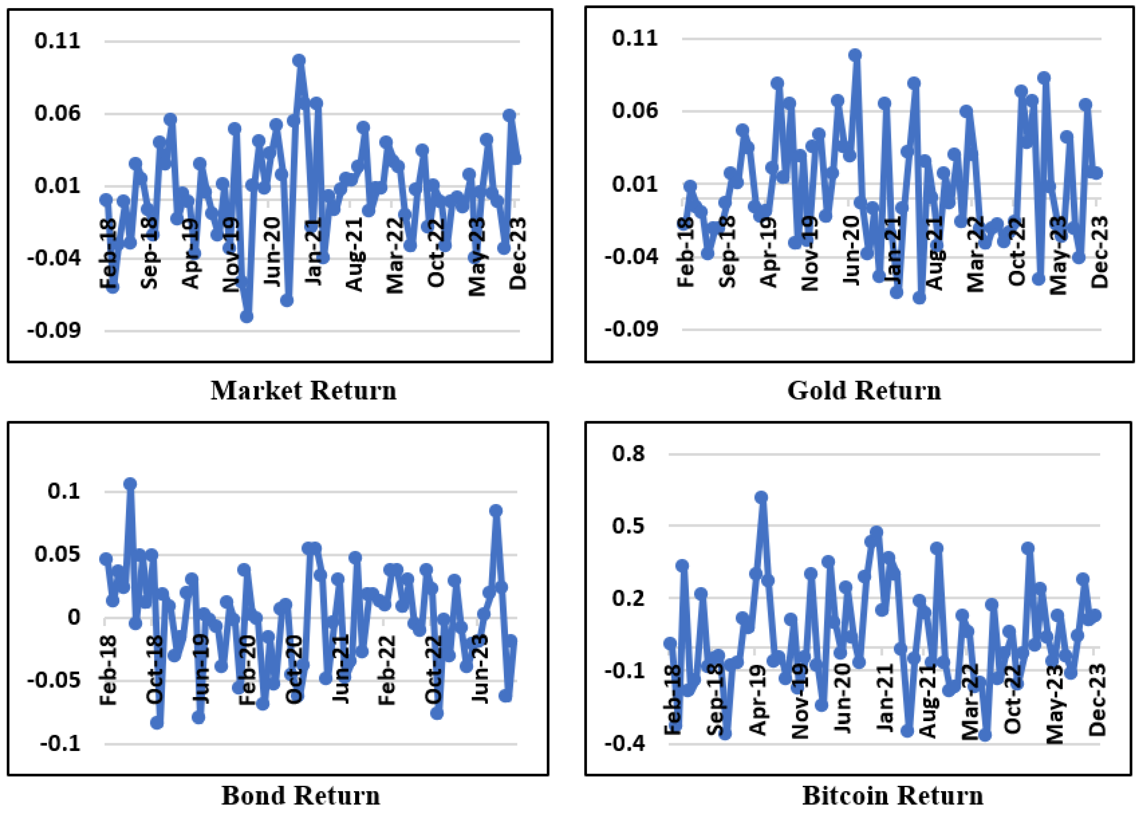
Figure 2.
Exc, Inf and SBI Surprise Factors. Note: The surprise factors were measured using the exponential smoothing method in EViews 13. The average returns for Act_Exc, Act_Inf, and Act_SBI are 0.0023, 0.0036, and 0.0039, respectively. The values for Pred_Exc, Pred_Inf, and Pred_SBI were obtained using the exponential smoothing method. The surprise factors for Exc, Inf, and SBI have averages of -0.0003, -0.0081, and 0.0001, respectively.
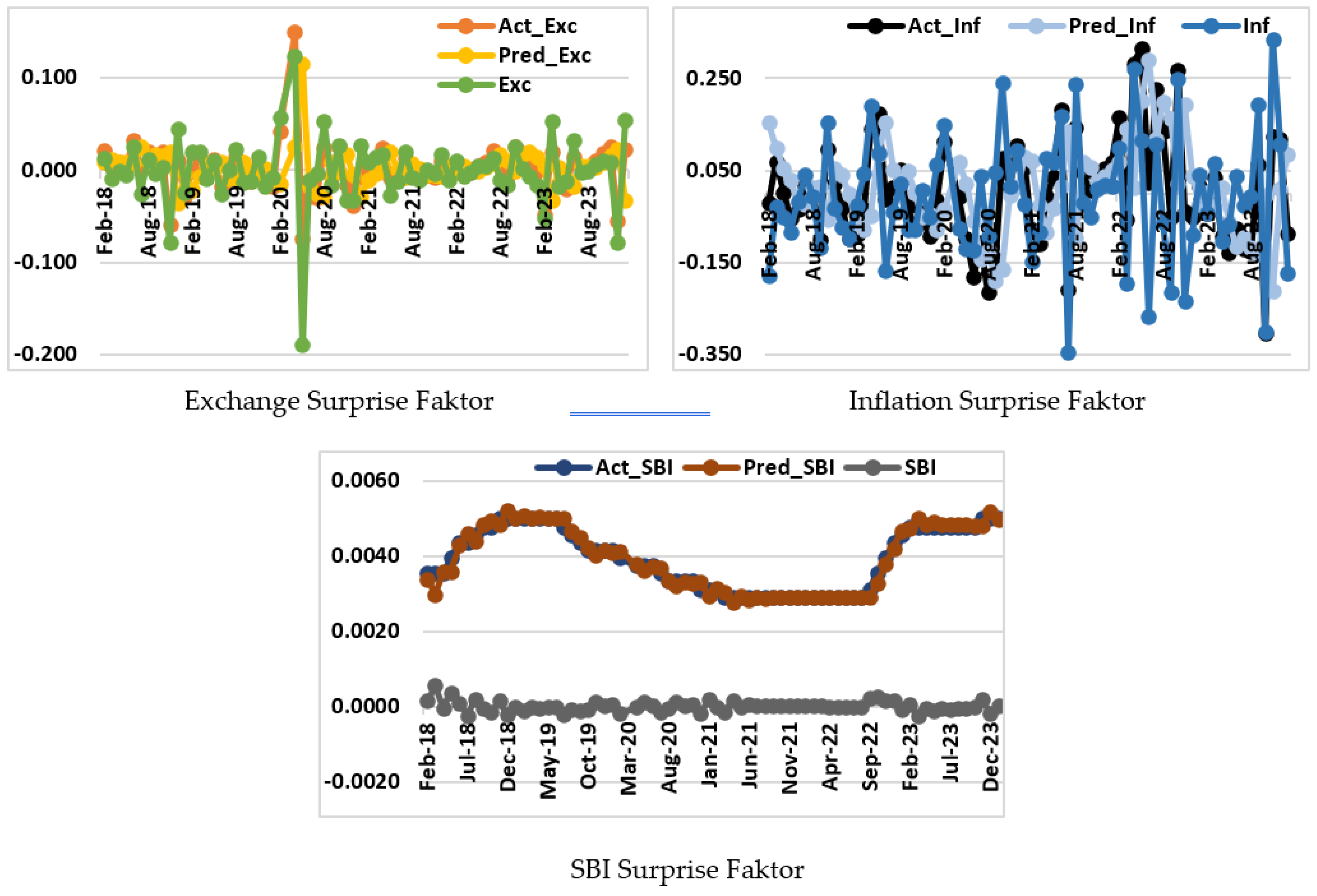

Table 1.
Variables Measurement Used In Analysis.
| Variable | Indicator | Measurement | Scale |
| Return of Investment ( | Rm (For Stock) Rg (For Gold) Rb (For Bond) Rbtc (For BTC) |
Ratio | |
| Volatility | Vm (For Stock) Vg (For Gold) Vb (For Bond) Vbtc (For BTC) |
Ratio | |
| Expected Return of Investment () | Erm (For Stock) Erg (For Gold) Erb (For Bond) Erbtc (For BTC) |
Ratio | |
| Inflation (Inf) | Consumer Price Index | Ratio | |
| Exchange Rate (Exc) | Rp/USD | Ratio | |
| Interest Rate (SBI) | SBI 1/Month | Ratio |
Table 2.
Analysis Descriptif of Dependent Variables.
| Rm | Rg | Rb | Rbtc | Vm | Vg | Vb | Vbtc | |
|---|---|---|---|---|---|---|---|---|
| Mean | 0.00214 | 0.00678 | 0.00124 | 0.04109 | 0.06447 | 0.06473 | 0.05868 | 0.30714 |
| Median | 0.00431 | -0.00368 | 0.00571 | 0.00023 | 0.05556 | 0.05855 | 0.05430 | 0.28614 |
| Max | 0.09442 | 0.09718 | 0.14811 | 0.60846 | 0.37480 | 0.16123 | 0.24220 | 0.81397 |
| Min | -0.16758 | -0.06996 | -0.08546 | -0.37325 | 0.02092 | 0.02326 | 0.02018 | 0.05971 |
| Std.Dev | 0.03925 | 0.03839 | 0.04251 | 0.21076 | 0.04581 | 0.02704 | 0.03194 | 0.15191 |
| Skew | -1.07506 | 0.34145 | 0.39031 | 0.35412 | 4.55218 | 0.98695 | 2.82187 | 0.96663 |
| Kurtosis | 6.76807 | 2.41795 | 4.12593 | 2.74918 | 30.84016 | 3.85904 | 16.58875 | 3.88144 |
| JB | 55.67995 | 2.38181 | 5.55307 | 1.66998 | 2538.14322 | 13.70969 | 640.49657 | 13.35514 |
Source: Processed by Author.
Table 3.
Analysis Descriptif of Independent Variables.
| Exc | Inf | SBI | |
|---|---|---|---|
| Mean | 0.00354 | -0.00304 | 0.00389 |
| Median | 0.00219 | -0.00671 | 0.00396 |
| Maximum | 0.03247 | 0.28155 | 0.00500 |
| Minimum | -0.02925 | -0.30275 | 0.00014 |
| Std. Dev. | 0.01372 | 0.11238 | 0.00094 |
| Skewness | -0.27401 | 0.17228 | -0.81621 |
| Kurtosis | 2.76637 | 3.23433 | 4.55215 |
| Jarque-Bera | 1.04992 | 0.51368 | 15.01046 |
Source: Processed by Author.
Table 4.
ADF Test Result For Unit Roots.
| Var | Level | 1st Differences | Var | Level | 1st Differences | ||||
| t-stat | Prob | t-stat | Prob | t-stat | Prob | t-stat | Prob | ||
| Rm | -7.6996 | 0.0000 | Vb | -3.8007 | 0.0045 | ||||
| Rg | -9.7548 | 0.0000 | Vbtc | -6.3534 | 0.0000 | ||||
| Rb | -7.8943 | 0.0000 | Exc | -9.4378 | 0.0000 | ||||
| Rbtc | -6.8974 | 0.0000 | Inf | -7.0533 | 0.0000 | ||||
| Vm | -5.4990 | 0.0000 | DSBI | -1.3716 | 0.5912 | -4.0015 | 0.0025 | ||
| Vg | -6.0199 | 0.0000 | |||||||
Source: Processed by Author. ADF Test has using maximum Lag = 11.
Table 5.
Granger Causality Tests.
| Return | F-Stat | Prob. | Volatility | F-Stat | Prob. |
| RIG does not Granger Cause RIM | 0.3011 | 0.8244 | VG does not Granger Cause VM | 0.0917 | 0.9125 |
| RIM does not Granger Cause RIG | 0.6822 | 0.5663 | VM does not Granger Cause VG | 1.7907 | 0.1751 |
| RIBTC does not Granger Cause RIM | 0.0755 | 0.9729 | VB does not Granger Cause VM | 0.1082 | 0.8976 |
| RIM does not Granger Cause RIBTC | 0.4695 | 0.7046 | VM does not Granger Cause VB | 0.8527 | 0.4310 |
| RIB does not Granger Cause RIM | 0.3643 | 0.7790 | VBTC does not Granger Cause VM | 1.1402 | 0.3262 |
| RIM does not Granger Cause RIB | 0.6212 | 0.6040 | VM does not Granger Cause VBTC | 3.7902 | 0.0278* |
| RIBTC does not Granger Cause RIG | 0.1360 | 0.9382 | VB does not Granger Cause VG | 0.3279 | 0.7217 |
| RIG does not Granger Cause RIBTC | 2.6551 | 0.0564* | VG does not Granger Cause VB | 0.6683 | 0.5161 |
| RIB does not Granger Cause RIG | 0.5266 | 0.6657 | VBTC does not Granger Cause VG | 0.2899 | 0.7493 |
| RIG does not Granger Cause RIB | 0.5285 | 0.6644 | VG does not Granger Cause VBTC | 0.8724 | 0.4228 |
| RIB does not Granger Cause RIBTC | 2.9582 | 0.0393* | VBTC does not Granger Cause VB | 1.0635 | 0.3513 |
| RIBTC does not Granger Cause RIB | 1.0512 | 0.3765 | VB does not Granger Cause VBTC | 0.8110 | 0.4489 |
| RIBTC does not Granger Cause RIG | 0.1360 | 0.9382 | VG does not Granger Cause VM | 0.0917 | 0.9125 |
Source: Processed by Author. Note: We have tested dependent variable accros other dependent variable using maximum lag 12. A variable denotes by * indicates that it is significant at a probability level greater than 0.05.
Table 6.
GARCH Estimation Result For Volatility Return and Price.
| C | Variance Equation | AIC | ARCH-LM | |||||
|---|---|---|---|---|---|---|---|---|
| C | GARCH(-1) | |||||||
| Rm | 0.0110 | -1.1436 | -0.0585 | 26.4462 | 5.35 x 10⁻⁵ | 0.9406 | -4.1887 | 0.7642 |
| (0.0149)** | (0.0000)* | (0.0124)** | (0.2640) | (0.1251) | (0.0000)* | |||
| Rg | 0.0106 | -1.3825 | 0.0098 | 22.8724 | 0.0002 | 0.9090 | -3.7734 | 0.3836 |
| (0.0002)* | (0.0000)* | (0.7905) | (0.3842) | (0.6420) | (0.0000)* | |||
| Rb | -0.0073 | 1.1910 | 0.0996 | -8.0945 | 0.0002 | 0.8131 | -3.8121 | 0.6161 |
| (0.0000)* | (0.0001)* | (0.0019)* | (0.6781) | (0.6705) | (0.0757)*** | |||
| Rbtc | 0.0516 | -2.7089 | -0.0870 | -272.4830 | 0.0045 | 0.8681 | -0.3092 | 0.7537 |
| (0.0990)*** | (0.0878)*** | (0.6692) | (0.2208) | (0.1251) | (0.0000)* | |||
| Vm | 0.0635 | 0.6521 | 0.0356 | -32.6773 | 0.0002 | 0.8372 | -3.5854 | 0.9900 |
| (0.0000)* | (0.0000)* | (0.6113) | (0.5360) | (0.5902) | (0.0097) | |||
| Vg | 0.0716 | 0.2296 | -0.0192 | -28.5638 | 5.73 x 10⁻⁵ | 0.9014 | -4.4426 | 0.4398 |
| (0.0000)* | (0.0018)* | (0.4951) | (0.1607) | (0.6071) | (0.0000)* | |||
| Vb | 0.0550 | 0.5453 | -0.0143 | -22.9669 | 0.0010 | -0.9956 | -4.5067 | 0.8507 |
| (0.0000)* | (0.0000)* | (0.5530( | (0.3016) | (0.0000)* | (0.0000)* | |||
| Vbtc | 0.2928 | 0.8612 | 0.2025 | -126.2299 | 0.0052 | 0.6690 | -0.9657 | 0.7759 |
| (0.0000)* | (0.4305) | (0.2426) | (0.5260) | (0.2951) | (0.0306)** | 0.7642 | ||
Table 7.
Quantile Regression For Return Volatility and Price Volatility.
| Dependent Variabel | Rm | Vm | Rg | Vg | |||||
| t | Var | Coeff Value |
Prob (>|t|) | Coeff Value |
Prob (>|t|) | Coeff Value |
Prob (>|t|) | Coeff Value |
Prob (>|t|) |
| 0.06 | C | -0.0410 | 0.0000* | 0.0279 | 0.0000* | -0.0356 | 0.0000* | 0.0344* | 0.0000* |
| Exc | -0.6564 | 0.0786*** | -0.1217 | 0.6675 | -1.1784 | 0.0080** | -0.1001 | 0.7013 | |
| Inf | -0.1700 | 0.0418** | 0.0213 | 0.3534 | 0.0913 | 0.0304** | 0.0102 | 0.7623 | |
| DSBI | -1.9816 | 0.7507 | -1.9240 | 0.9450 | 12.0044 | 0.0292** | -26.8948 | 0.4161 | |
| 0.07 | C | -0.0370 | 0.0006* | 0.0285 | 0.0000* | -0.0329 | 0.0000* | 0.0346 | 0.0000* |
| Exc | -0.6149 | 0.0931*** | -0.1558 | 0.5963 | -1.4104 | 0.0060* | -0.0925 | 0.7205 | |
| Inf | -0.1542 | 0.0700*** | 0.0248 | 0.2760 | 0.1435 | 0.0030* | 0.0087 | 0.7966 | |
| DSBI | -3.5243 | 0.5584 | -1.7859 | 0.9561 | 10.3931 | 0.0431* | -25.6888 | 0.4323 | |
| 0.8 | C | 0.0313 | 0.0000* | 0.0901 | 0.0000* | 0.0397 | 0.0001* | 0.0895 | 0.0000* |
| Exc | -0.5685 | 0.1566 | 0.4154 | 0.1525 | -0.9859 | 0.2467 | 0.3912 | 0.0012* | |
| Inf | -0.0901 | 0.0616*** | 0.0397 | 0.6479 | -0.0429 | 0.5986 | -0.0294 | 0.4427 | |
| DSBI | -25.0122 | 0.0000* | -62.3997 | 0.0515** | -7.6494 | 0.2492 | -42.3748 | 0.1972 | |
| 0.9 | C | 0.0454 | 0.0000* | 0.1005 | 0.0000* | 0.0692 | 0.0000* | 0.1041 | 0.0000* |
| Exc | -0.4210 | 0.3916 | 0.4511 | 0.0862*** | -0.2675 | 0.7658 | 0.3350 | 0.0033* | |
| Inf | 0.0270 | 0.7854 | 0.0479 | 0.5362 | -0.0934 | 0.2524 | -0.0307 | 0.4649 | |
| DSBI | -31.6940 | 0.0000* | -86.8034 | 0.0040* | -16.0449 | 0.0153** | -32.0841 | 0.3146 | |
| 0.06 | C | -0.0700 | 0.0000* | 0.0225 | 0.0000* | -0.2169 | 0.0000* | 0.1189 | 0.0000* |
| Exc | 0.6530 | 0.3872 | -0.1344 | 0.6830 | 0.3539 | 0.8385 | 0.7638 | 0.5790 | |
| Inf | 0.0351 | 0.7639 | -0.0169 | 0.6404 | -0.7267 | 0.0086* | 0.3461 | 0.0066* | |
| DSBI | -35.7577 | 0.8509 | 28.8965 | 0.4918 | -28.3947 | 0.4270 | -25.0035 | 0.8578 | |
| 0.07 | C | -0.0266 | 0.0001* | 0.0225 | 0.0000* | -0.2169 | 0.0000* | 0.1291 | 0.0000* |
| Exc | 1.3275 | 0.0128* | -0.1344 | 0.7236 | 0.3539 | 0.8393 | 0.8531 | 0.5065 | |
| Inf | 0.0397 | 0.6265 | -0.0169 | 0.6993 | -0.7267 | 0.0071* | 0.3007 | 0.0111* | |
| DSBI | 8.9263 | 0.1766 | 28.8965 | 0.5518 | -28.3947 | 0.3869 | -25.5275 | 0.8520 | |
| 0.8 | C | 0.0210 | 0.0002* | 0.0745 | 0.0000* | 0.2164 | 0.0000* | 0.4306 | 0.0000* |
| Exc | 1.3460 | 0.0045* | 0.2550 | 0.1505 | -3.0241 | 0.2960 | -0.0050 | 0.9982 | |
| Inf | -0.0040 | 0.9337 | -0.0057 | 0.8928 | 0.2997 | 0.4073 | 0.5095 | 0.2794 | |
| DSBI | -4.2278 | 0.4298 | 52.2871 | 0.0357** | -163.3711 | 0.0001* | -197.3619 | 0.3792 | |
| 0.9 | C | 0.0328 | 0.0000* | 0.0927 | 0.0000* | 0.3496 | 0.0000* | 0.5170 | 0.0000* |
| Exc | 1.2332 | 0.0017* | 0.5000 | 0.0356** | -1.9785 | 0.6078 | 0.8943 | 0.1776 | |
| Inf | -0.0888 | 0.0232* | -0.0047 | 0.9564 | 0.1064 | 0.8703 | 0.3080 | 0.4548 | |
| DSBI | -5.8383 | 0.2843 | 5.5794 | 0.8765 | -199.7364 | 0.0000* | -390.8188 | 0.0399** | |
Source: Processed by Author. Note: In the context of regression analysis, the constant term CCC is interpreted as the expected return in the return regression model, and as the expected volatility in the volatility regression model. The coefficient values quantify the impact of the independent variables on the dependent variable. The probability values (>|t|) indicated the significantof the coefficient. A * denotes significance at the 1% level, ** denotes significance at the 5% level, and *** denotes significance at the 10% level.
Table 8.
Cross Sectional Result.
| Variable | Coefficient | Std. Error | t-Statistic | Prob (>|t|) |
| C | 0.00057 | 0.00716 | 0.07902 | 0.93710 |
| DRf | 13.95689 | 31.68150 | 0.44054 | 0.66004 |
| Exc | -0.24017 | 0.10505 | -2.28620 | 0.02333** |
| Inf | -0.19006 | 0.02962 | -6.41658 | 0.00000* |
| DSBI | 20.94218 | 23.31436 | 0.89825 | 0.37017 |
Source: Processed by Author. Note: The analysis was conducted using panel data OLS with the Fixed Effect Model approach. To address issues of heteroskedasticity and autocorrelation, we applied specific weights to the observations (GLS Period Weight). The model successfully passed the classical assumption tests required for the above methods. The prob (>|t|) indicates the probability values, where values marked with * denote variables significant at the 1% level, and those marked with ** indicate significance at the 5% level.
Table 9.
Expected Return And Loading Factors.
| Er | |||||||
|---|---|---|---|---|---|---|---|
| Rm | 0.011 | -1.1436 | -0.0585 | -0.2402 | -0.1901 | ||
| Rg | 0.0106 | -1.3825 | -0.2402 | -0.1901 | |||
| Rb | -0.0073 | 1.191 | 0.0996 | -0.2402 | -0.1901 | ||
| Rbtc | 0.0516 | -2.7089 | -0.2402 | -0.1901 |
Source: Processed by Author.
Table 10.
Optimal Portfolio.
| Instrumen | Old Portfolio | Arbitrage Portfolio | Optimal Portfolio |
| Saham | 25% | 0.03 | 28% |
| Emas | 25% | -0.0872 | 16% |
| Obligasi | 25% | 0.0176 | 27% |
| BTC | 25% | 0.0396 | 29% |
Source: Processed by Author.
Disclaimer/Publisher’s Note: The statements, opinions and data contained in all publications are solely those of the individual author(s) and contributor(s) and not of MDPI and/or the editor(s). MDPI and/or the editor(s) disclaim responsibility for any injury to people or property resulting from any ideas, methods, instructions or products referred to in the content. |
© 2024 by the authors. Licensee MDPI, Basel, Switzerland. This article is an open access article distributed under the terms and conditions of the Creative Commons Attribution (CC BY) license (https://creativecommons.org/licenses/by/4.0/).
Copyright: This open access article is published under a Creative Commons CC BY 4.0 license, which permit the free download, distribution, and reuse, provided that the author and preprint are cited in any reuse.


