Submitted:
08 August 2024
Posted:
14 August 2024
You are already at the latest version
Abstract
Interaction between multiple phases especially liquid-gas is one of the most common phenomena in industrial systems. Computer Vision enables modern systems to derive an automated and robust image-processing technique to address this issue. However, diverse experimental conditions still make it a challenging task to overcome. In Deep Learning, instance segmentation has created a niche in various computer vision applications as it aims to provide different instance IDs to objects belonging to the same class. In this paper, we propose a novel approach employing the YOLO (You Look Only Once) an end-to-end deep learning architecture for the detection and segmentation of bubbles in fluid flows. YOLOv5 offers significant improvements in both speed and accuracy compared to its predecessors like YOLOv3. Therefore, we train the YOLOv5 network on a dataset consisting of annotated images representing instances of bubbles across varied fluid flow environments. This paper provides both qualitative and quantitative evaluation of three YOLOv5 networks (small, medium, and extra-large) in detecting and segmenting bubbles with high accuracy and efficiency. Based on the metrics all three YOLOv5 models achieved high precision above 0.98 for bounding box detection and 0.97 for segmentation mask, and high recall value greater than 0.97 for box and 0.96 for mask quality was achieved. The achieved results indicate that the models accurately localize bubbles within the image frame, and distinguish bubble pixels from the background. Also, mean average precision (mAP50-95) consistently exceeds 0.84 across all models for the bounding box and 0.73 for the segmentation mask. The ascertained results emphasize the potential of YOLOv5 architecture as a powerful tool for automated bubble analysis in real-world applications. Our research contributes to advancing the field of deep neural networks in fluid systems and provides a fresh approach for future developments in automated bubble analysis.
Keywords:
Computer-Vision
; Image-Processing
; Object-Detection
; Instance-Segmentation
; YOLO
; Artificial Neural Networks (ANNs)
; Deep Learning
; Fluid Flows
; Bubbles
1. Introduction
In a multiphase flow system interaction between more than one phase takes place. The most common multiphase flows are Two-Phase flows like Gas-Solid, Gas-Liquid, Liquid-Liquid, and Liquid-Solid flows. The scenario addressed in this paper is about the Liquid-Gas phase. Purging gas is employed in cases where mechanical stirring is restricted due to high temperatures or economic reasons. Detailed knowledge regarding the Liquid-Gas phase in this case water-bubble flow characteristics and dynamics is imperative for process optimization. The distribution of bubble size plays an important role in thermodynamic reactions and numerical flow models. Knowledge regarding the interaction between liquid bubbles is important for determining the quantity of energy transferred during the mixing process. Determining the flow characteristics of bubbles can also help in validating several numerical models [1]. There are several flow measurement techniques available covering various applications, which are mainly divided into two parts intrusive and non-intrusive methods. As the name suggests in intrusive methods a physical probe is inserted into the flow of the fluid and then its flow characteristics are measured. On the other hand, non-intrusive methods do not obstruct the fluid flow and therefore does not affect the phenomena to be examined. Most widely used methods like Laser Doppler Velocimetry (LDV) [2], helps in measuring flow fields, while, Shadowgraph experiments [3], helps in study convection patterns in dissipative nonequilibrium systems, shadowgraphs are employed to study fluctuations close to but below the onset of convections at much smaller wave numbers. Whereas, methods like Particle Image Velocimetry (PIV) [4], measures displacements of known particles during two consecutive laser flashes. Generally, PIV provides less spatial and temporal resolutions than LDV method, except when using high speed laser and cameras. Specific to the condition of liquid-bubble interaction, bubble characteristics like coordinates, shape, and size can be ascertained by using multi-staged pixel intensity level approaches by employing traditional image processing and computer vision techniques [5,6,7,8,9]. A general shortcoming of traditional image processing techniques is that the parameters during the different stages of flow are dependent on the experimental conditions during which the images were captured. Recent enhancements in computing power and sensor capability have helped deep learning to achieve greater accuracy in tasks such as image classification, object detection, and segmentation as compared to traditional image processing techniques like Support Vector Machine (SVM) [10], K-Nearest Neighbor [11], Naive Bayes Algorithm [12].
Deep Learning: The term deep learning is essentially associated with a neural network with multiple hidden layers generally three or more. These neural networks try to simulate the actions of the human brain and attempt to learn from the large amount of data. The training data, weights, and bias in combination empower a neural network to classify and recognize objects within the dataset with good accuracy and precision. Deep neural networks consist of multiple hidden layers of interconnected nodes, each layer builds upon the previous layer to optimize the prediction. The data is fed into the input layer for processing and the output layer is where the final prediction or classification is made, and the progression of information through the network is termed as forward propagation. Another important process of neural networks is backpropagation in which the network uses algorithms like gradient descent to compute errors in predictions and accordingly adjusts the weights and biases of the function by backpropagating through the layers and hence training the model. In combination forward and backpropagation iteratively makes a model more accurate by making predictions and correcting the errors accordingly.
Object Detection: Object detectors help to detect the coordinates of any object class with a recognized label. Object detectors are divided into two main categories: one-stage, and two-stage detectors. One-stage detectors follow an end-to-end process in which the localization of the bounding boxes and their class labels are determined. Whereas, in the case of two-stage detectors, in the first stage a region proposal network (RPN) is employed to extract the features from each candidate box for bounding-box regression while recognition is carried out in the second stage. The most commonly used two-stage object detector is Faster R-CNN [13], which was proposed to improve R-CNN [14], and Fast R-CNN [15]. Faster R-CNN uses a fully convolutional region proposal network (FCRPN) to predict the bounding box efficiently and hence achieved mean average precision (mAP) of 73.2% with 7 frames per second (FPS) on the PASCAL VOC 2007 and 2012 train-validation dataset. YOLO [16], and SSD [17], are the most commonly used one-stage object detectors. In this paper, we test the capabilities of YOLO so it is imperative to know how it processes the input image. First, the image is divided into S x S grid cells, these cells are in charge of detecting N objects whose centers lie within them. Every grid cell predicts N bounding boxes represented using x, y, w, h where x and y are coordinates whereas w, h is the width and height of each box respectively. Object localization and recognition are achieved with the help of 24 convolutional layers in the backbone, followed by two fully connected layers. YOLO [16] achieved mAP of 63.4% with 45 FPS on the PASCAL VOC dataset. A series of optimizations in architecture with increased bounding boxes were proposed in YOLOv2 [18], and YOLOv3 [19]. A detailed description of YOLOv5 [20], architecture is provided in the methodology section below.
Instance Segmentation: In instance segmentation both object detection and semantic segmentation take place simultaneously. The process flow starts with predicting the instances of the object class followed by a binary segmentation mask. In two-stage instance segmentation methods, the process starts with detection of the bounding box followed by a binary segmentation of each detections. In case of two-stage detectors like Mask R-CNN [21], in which an additional branch is added to Faster R-CNN architecture, which eventually computes the segmentation mask to the detected object by using Region of Interest (RoI) Align instead of Region of Interest (RoI) Pooling. The above-mentioned changes achieved better accuracy when the loss function combines the computed losses of the bounding box, recognized class, and the segmented mask. Further improvements are achieved in PANet [22], and Mask Scoring R-CNN [23]. In one-stage detectors, both detection and segmentation are performed directly. In InstanceFCN [24], a fully convoluted network is used to produce multiple instance-sensitive score maps that carry details of the relative location followed by a proposal of object instances generated employing an assembling module. One of the first attempts for real-time instance segmentation was YOLOACT [25], which used a feature backbone followed by two parallel branches, where the first branch produces several prototype masks and the second branch computes mask coefficients for each instance of the object class. The produced prototype masks and their associated mask coefficients are combined linearly, and finally, a concluding object instance is produced by cropping and thresholding operation. YOLOACT achieved mAP of 29.8% on the COCO dataset at 33.5 FPS using Titan Xp GPU. Several other methods were also released like YOLOACT++ [26], and INSTA-YOLO [27], with improved designs that addressed the same case.
Related Work: The use of computer vision techniques to investigate bubbly flows as a non-intrusive method has gained some popularity in recent years. However, the complexity of bubble overlapping, and dense bubble swarms can make image processing and evaluation a tedious task. This issue is addressed in depth by Yucheng Fuâs dissertation [28]. The most widely tried approach to solving this problem is the identification of bubbles by detecting the anchor points within a bubble which is generally the center point. Using a CNN-based sliding window approach to approximate anchor points is explored by Poletaev et al., [29]. BubCNN [1], uses Faster R-CNN [13], and proposes anchor points with matching bounding boxes around detected bubbles. In the case of overlapping bubbles, another approach is to directly predict a segmentation mask for an image using down-and-upsampling CNN by classification and assigning each pixel to specific objects. A customized Mask-RCNN version was used by Kim and Park [30], which directly offers a segmentation mask as the output. All of the above-mentioned methods identify bubbles, and ellipsoidal fit segments and reconstruct the object resolving the tasks of segmentation and reconstructing overlapping bubbles. In BubCNN [1], a CNN-based shape regression model fits an ellipse around the detected bubble. Another approach to using CNN for pixel-pixel predictions to identify and segment bubbles is explored by Hessenkemper et al., [31], where different approaches were examined to evaluate gas volume fraction and bubble sizes. In this work, we adopt the strategy to use YOLOv5 [20], algorithm with many practical advantages over the previous versions like YOLOv3 [19], for the faster detection and instance segmentation of bubbles in the liquid-gas multiphase flow system.
2. Materials and Methods
In this section, detailed information about the YOLOv5 model is provided, starting with datasets, followed by the network architecture, metrics, and finally the training setup.
Datasets: In this paper, the YOLOv5 model was trained and evaluated on the dataset generated and used in BubCNN [1], the dataset was created for different experimental conditions such that both shape regression CNN and Faster R-CNN can be used. The dataset was acquired in four parts encompassing different experimental conditions such that a diverse set of datasets is ascertained. The first quarter of images were extracted from a 1:5 water model of a steel casting ladle using a highspeed video of bubble swarms, where the model cylinder with a diameter of 0.64 meters was filled up to a height of 0.646 meters. A porous plug with a diameter of 0.02 meters placed at the eccentrical radius of 0.21 meters was used to generate bubbles. By varying certain physical parameters like the aperture of the camera, the distance between the camera and the bubble column helped with acquiring a diverse set of data. In the above-mentioned case, the average equivalent bubble size is between 3-5 mm with a void fraction up to 0.07 as per trial conditions. Also, the bubble column fluctuates radially resulting in blurring of the recorded bubble outlines. The second quarter of the data was acquired from the experiment of the rise of single bubbles in different water-glycerin mixtures where the size of the bubble ranged between 2-8 mm. The images were captured by using two different highspeed cameras namely Photron FASTCAM SA3 and Dalsa Genie Nano M1280. The third quarter was generated artificially by random modification of the existing data. This process helps in increasing the diversity of the dataset by incorporating various techniques like data augmentation namely, adding noise to raw data, blurring of images by a Gaussian filter, and random intensity adjustment. The last quarter was generated synthetically using BubGAN [32], which is based on the measurement of a bubble swarm with a void fraction of 0.1, where the average equivalent size of the bubble is approximately 3 mm. Several bubble parameters like swarm density, size distribution, and background intensity were randomly varied in a relatively small water model. Figure 10, Figure 11, Figure 12 and Figure 13, show some of the images from the dataset encompassing a diverse set of bubbles under diverse experimental conditions.
To train a deep learning model like YOLO for object detection tasks, ground truth needs to be represented by a bounding box in which the center, width, and height coordinates are defined during the process of data labeling. On the other hand, segmentation ground truth is generally provided as dense pixel-wise annotation. In this paper, instance segmentation is performed where prediction of the polygon of each object instance in this case bubble is carried out through the center of the object. Systematically in the process flow of pattern recognition, four constituent pillars are perceived, namely data collection, data preprocessing, feature extraction, and finally classification or prediction. The first step i.e. data collection is discussed above, which brings us to the next step of data preprocessing. As discussed earlier for training YOLO, ground truth is required for instance segmentation which in simple terms means the raw images should be labeled with the exact coordinates of each object present in an image such that the algorithm learns from marked objects in the form of polygons during the training process. Generally, working with custom datasets like bubbles, in this case, requires manual labeling of each bubble using labeling tools to generate XML files which is a simple machine data serialization format file designed for human-machine interaction. The dataset is represented in XML files along with corresponding images which contain the information of the labeled objects. Manual labeling of hundreds of images seems like an achievable task if time is no constraint but custom datasets that comprise thousands of images with single and multiple bubbles in a single image seem like an enormous task, hence data scientists and engineers often use transfer learning to reuse the pre-trained model on a completely new platform such that the knowledge gained from a prior project can be applied to detect or predict about a new task. For this purpose, Segment Anything (SA) [33], a deep learning algorithm introduced by Meta AI Research was employed which enables zero-shot generalization to unfamiliar objects and images without requiring additional training. The model is designed, trained, and evaluated on numerous problems and the zero-shot performance was found to be impressive. The pre-trained weights of the Segment Anything model can be accessed from the GitHub repository [33], the model checkpoint- and specific model type- , was compiled in Python environment using Visual Studio Code to segment raw images of our custom datasets. The images are labeled using , running on CUDA mode. The specific details of hardware configuration for this project will be provided in the section on training setup. The pre-trained weights of the SA model generate masks for segmenting the input images with user-defined object classes. In our case we have only one class i.e. bubbles. The generated mask consists of a list of masks, where each mask is a dictionary containing information about the same, Figure 1, provides a detailed view of the properties of the generated masks.
Although auto-labeling reduces the amount of time required for manual labeling greatly due to the transfer learning module incorporated for the case this comes with its challenges. For example, in some of the labeled images some bubbles are labeled multiple times or many false positives are encountered as well. A possible reason for this might be that the Segment Anything model is an automatic mask generation algorithm. It does not require a class object to be specified but learns by itself about the features from the input images. Therefore, visualizing the labeling of bubbles and manual correction of the same becomes imperative for the ascertainment of a quality dataset. For this purpose, Roboflow [34], an end-to-end computer vision tool was employed, which empowers data engineers to develop a computer vision project. It helps to upload, organize, collaborate, and label datasets which can be further used for training a deep learning algorithm. In our case, Roboflow [34], was used to manually correct the mislabeled bubbles and finally create an appropriate custom dataset for training the PyTorch-based YOLOv5 model for instance segmentation. The entire workflow of ascertainment of the custom dataset is shown in Figure 2.
Network Architecture: "You Only Look Once" is an object detection method where an input image is treated in its entirety, which makes it different from the âsliding windowâ approach in which the specific segments of an image are classified individually. YOLO permits faster processing of data features because it does not have to perform several independent evaluations. This approach helps in achieving improved accuracy because the total image framework is made accessible to the entire network architecture. YOLO [16], was first released in 2018, and since then it has improved with multiple releases YOLOv2 [18], and YOLOv3 [19]. YOLOv5 [20], is an improved version of YOLO detection architecture that employs several optimization strategies in the context of convolutional neural networks (CNNs) such as mosaic data augmentation [36], self-learning bounding box anchors, and the cross-stage partial network. YOLO was the first object detection network that provided an end-to-end connection between the process of predicting bounding boxes with class labels of the objects.
The architecture consists of three main pillars: a backbone network, a detection neck, and output. It employs advanced methods such as BottleneckCSP based on CSPDarknet53 [36], Spatial Pyramid Pooling (SPP) [36], and PANet to boost object detection. Figure 3, explains a basic workflow of YOLOv5 architecture. It commences at the input terminal with data preprocessing tasks such as mosaic data augmentation [37], and adaptive image filling. YOLOv5 also incorporates adaptive anchor frame calculation on the input, which makes it feasible for a variety of dataset by automatic generating an initial anchor frame size. The backbone of YOLOv5 is a convolutional neural network (CNN), where feature extraction of different sizes from an input image is achieved with the help of a spatial pyramid pooling (SPP), and a cross-stage partial (CSP) network. To reduce the amount of calculation and achieve a higher rate of inference BottleneckCSP is used, whereas SPP helps in feature extraction from different scales for the same feature map. It can generate three-scale feature maps which eventually helps in achieving better detection accuracy. The detection neck network incorporates the advantages of feature pyramid structures of FPN [38], by using its semantic features from the top to lower feature maps as well as using the localization features of PAN [39], from lower to higher feature maps to improve the feature extraction property of the network. Finally, the head output is used to predict targets of diverse dimensions on the feature maps. A detailed and descriptive explanation of the model architecture can be found on the website of Ultralytics [20]. Ultralytics provides 5 individual architectures for segmentation namely YOLOv5n-seg, YOLOv5s-seg, YOLOv5m-seg, YOLOv5l-seg, YOLOv5x-seg. The difference between these architectures is built on the grounds of the number of feature extraction modules and convolution kernels.
Table 1, provides the quantitative results of the study of the above-mentioned architectures when trained on the COCO dataset for 300 epochs at image size 640 using A100 GPUs. A piece of detailed information regarding the model performance can be found on the following GitHub repository [20]. In this paper YOLOv5s-seg, YOLOv5m-seg, YOLOv5x-seg model will be employed as the study requires a considerable amount of accuracy in the detection and segmentation of bubbles.
Accuracy, Losses, and Metrics: In deep learning, every model or architecture is evaluated both qualitatively and quantitatively. In this section a detailed description of some of the quantitative metrics is discussed:
IoU: âIntersection over Unionâ (IoU, IU) is one of the most important metrics used for object detection. IoU is represented in the form of an equation:
where A is the set of proposed object pixels and B is the set of true object pixels. In definition, IoU is the ratio between the area of overlap and the area of union. Figure 4, provides an overview of the area of overlap which is calculated between the predicted bounding box and the ground-truth bounding box. Whereas, the area of union is the area encompassed by both the ground-truth and predicted bounding box. Generally, if the value of IoU is greater than the threshold value of 0.5 it is considered a hit; otherwise, if the value of IoU is less than 0.5 it is a fail detection.
Confusion Matrix: An object detection task is evaluated by several standard metrics namely Precision, Recall, F1-score and Mean Average Precision (mAP) when the threshold value of IoU is 0.5. These metrics are computed based on the Confusion Matrix shown in Figure 5. A predicted bounding polygon is considered as a true positive (TP), when it overlaps more than the IoU threshold value with a labeled bounding polygon, else it is considered a false positive (FP). Likewise, when the value of IoU of the labeled bounding polygon with a predicted bounding polygon is lower than the threshold is considered as a false negative (FN). Precision is the ratio of correctly detected objects to the total number of detected objects, whereas, Recall is the ratio of correctly detected objects to the total number of objects in the dataset. Mean average precision (mAP) is the indication of the model evaluation under different confidence thresholds. F1-score is important for tasks like segmentation as it combines both Precision and Recall with equal weight as it offers a trade-off between Precision and Recall. Generally, increasing Precision reduces Recall and vice versa, this is where F1-score calculates the harmonic mean of both metrics and thus attaining a high score implies maximizing both Precision and Recall. The metrics are defined as:
Another significant improvement in YOLOv5 compared to previous versions is in the strategy to improve box prediction. In YOLOv5, the box coordinates were directly predicted using the activation of the last layer with a modified formula to reduce the grid sensitivity. Figure 6, shows the mechanism behind the same. The losses are computed using Binary Cross Entropy (BCE) which compares the predicted result of a classification model and the ground truth. The equation below describes the mathematical representation of BCE where , is the predicted value whose value is closer to 1, then the value of the loss function should be closer to 0, therefore the aim is to reduce the difference between the predicted and the ground truth value.
According to the Ultralytics webpage for YOLOv5, the loss is calculated as a sum of three individual components namely: Classes Loss (BCE), Objectness Loss (BCE), and Location Loss (CIoU) where the first two are BCE and the last one is an IoU loss. The mathematical representation of the overall loss function is shown in the equation below, where the class loss is the measure of the error for the classification task, objectness loss is the measure of the error in the detection of an objectâs presence in a particular grid cell, and finally, the location loss is the measure of the error in object localization within a grid cell. A detailed explanation of losses is provided on the official Ultralytics [20] website for YOLOv5.
Training Setup: The experiment deploys Python 3.8.10 and torch 1.9.0+cu102 deep learning framework for YOLOv5 model training and testing on a system with an Intel(R) Xeon (R) W-2155 CPU @ 3.30GHz, 64-bit with 128GB installed RAM, NVIDIA Quadro RTX 6000 24Gb GPU graphics card in Windows 11 operating system with VS Code version 1.89 as source-code editor. Incorporating the general procedures for network training on the YOLOv5 platform, this paper presents comprehensive information regarding multiple YOLOv5s, YOLOv5m, and YOLOv5x segmentation models on the dataset containing different experimental cases of bubbles. The dataset comprises 5820 images in total and Roboflow [34], was used to create a Train-Validation-Test split using a 70-20-10 % ratio. The image resolution size is 640*640 pixels, and the core hyperparameters values and functions involved in the training model are shown in Appendix Table A1. Parallel training of each segmentation model was carried out, on one hand by using the pre-trained weights from the Ultralytics YOLOv5 GitHub repository [20] and second by random weight initialization technique for training the models from scratch. Each model was trained for 300 epochs with default hyperparameters listed in Appendix Table A1. The trained models were evaluated on the validation dataset for the calculation of metrics and losses like Precision, Recall, mAP50 (computed value of mAP for minimum IoU threshold of 0.5), and mAP50-95 (mAP averaged over IoU thresholds from 0.50 to 0.95 at 5% steps), presenting comprehensive view of the model’s performance across different levels of detection difficulty. The ascertained results showed that the pre-trained models performed slightly better than the models trained from scratch for all three configurations of YOLOv5s, YOLOv5m, and YOLOv5x with the difference of metrics between 1.5 - 3%. Therefore, it is better to use the pre-trained model configurations, as transfer learning is faster and more efficient although bubbles were not part of the training data in the COCO dataset. Still, it empowers the model to focus on learning the specifics of the new object class i.e. bubbles, resulting in the efficient training process. On the other hand, training from scratch forces the model to learn everything including low-level features, although an advantage of this approach is a better generalization. The workflow for the above-mentioned approach is depicted in Figure 7. Therefore, it was decided that the pre-trained models with transfer learning advantages would be employed for further experiments.
An important aspect of training in deep learning architectures is batch-size or in simple words it refers to the number of samples used to update the network weights at each iteration. Larger batch sizes e.g., 32 or 64 may provide more accurate gradient estimates but requires more memory and computation power. On the other hand, smaller batches e.g., 4 or 8 are faster to train but may lead to deafening updates and potentially inferior convergence. Finding the optimal batch size depends on the dataset, hardware, and desired output. Ultralytics [20], addressed this issue for YOLOv5 by experimenting to monitor the effects of varying batch sizes on model training for YOLOv5s on the COCO dataset for 300 epochs with 8 different batch sizes: (16, 20, 32, 40, 64, 80, 96, 128) respectively.
Developers at Ultralytics tried to make the train code batch-size agnostic so that users ascertain similar results at any batch size. This was achieved by scaling loss, and weight decay with batch size. For batch sizes below 64, optimization of losses was delayed until the batch was complete. Conversely, losses were optimized after processing each batch when the size exceeded 64. To validate the results for the bubble dataset, different batch sizes (16, 32, 1) were selected for the YOLOv5 models for the train-validation-test split.
Figure 8, depicts the training and validation loss (box, seg, obj) curves for the pre-trained YOLOv5 models (s, m, x). The y-axis represents the loss value, and the x-axis represents the best epoch for each model configuration respectively. Detailed information regarding the model summary is provided in Table 2. The graph depicts three categories of loss namely box loss, segmentation loss, and object loss. Ideally, as the number of epochs increases, the training and validation loss tends to decrease, which points to the fact that the model is learning to perform better on the task of object detection and segmentation. In general, the training loss curve should smoothly decrease toward zero, while the validation loss curve may plateau after a certain number of epochs. A gap between the training and validation loss suggests that the model may be overfitting on the training data. An important observation about the graphs depicts that the segmentation loss (seg_loss) appears to be higher than the box loss (box_loss) and object loss (obj_loss) for all three models. This means that segmenting objects is more challenging than detecting and classifying bounding boxes around bubbles. In comparison to all three models, YOLOv5s appears to have the highest training loss curves, while validation loss curves for box loss plateaus, whereas the segmentation loss and object loss for YOLOv5x is more as compared to YOLOv5m and least for YOLOv5s.
Figure 9, depicts the qualitative results for YOLOv5 modelâs evaluation on the validation dataset, evaluation metrics like Precision, Recall, mAP50, and mAP50-95 (Y-axis) for both bounding box and segmentation mask for the best epoch (X-axis) respectively. Based on the graph YOLOv5m and YOLOv5x outperform the YOLOv5s model across all metrics by a very small margin. Table 3, presents the quantitative results for the above-mentioned metrics with the best metric being highlighted in the table.
3. Results & Discussion
This section presents the qualitative and quantitative evaluation of the above-trained YOLOv5 models for the detection and segmentation of bubbles on the test dataset. For rigorous testing of the models and evaluation of generalization capabilities, the test dataset contains a variety of scenarios for bubbles. Table 4, shows the quantitative results of the YOLOv5 models employing the standard metrics to assess both detection accuracy and segmentation mask quality with the best metric value highlighted for the three models. It is evident that all three YOLOv5 models (s, m, x) achieved high precision above 0.98 for bounding box detection and 0.97 for segmentation mask, and a similar result can be seen for recall where it achieved more than 0.97 for box and 0.96 for mask quality as well. This is a strong indication that the models accurately localize bubbles within the image frame, and accurately distinguish bubble pixels from the background, this can be explained by the value mAP50-95 consistently exceeding 0.84 across all models for the bounding box and 0.73 for the segmentation mask. Finally, model performance comparison based on the above-mentioned metrics shows that all models exhibited high performance, it is evident that YOLOv5s appears to have a slightly lower mAP compared to YOLOv5m, and YOLOv5x. This points to a minor trade-off between model size and segmentation mask precision.
A qualitative investigation of the model capabilities is shown in Figure 10, Figure 11 and Figure 12, highlighting three scenarios from the test dataset regarding bubbles with small, medium, and large sizes respectively. The first column displays the raw images, and the subsequent columns show the results obtained using YOLOv5s, YOLOv5m, and YOLOv5x, respectively. In Figure 10, it is evident that segmentation mask quality is almost the same for each model with minor differences but an important observation for the third row where YOLOv5s detects a false positive (FP). Similarly, in Figure 11, in overlapping bubble flow, the shape of the segmentation mask in YOLOv5m, and YOLOv5x is slightly better than YOLOv5s. Similar results can be observed in Figure 12, as well for large bubble sizes in terms of mask shape and quality. Figure 13, shows the performance comparison of YOLOv5 models (s, m, x) for bubble detection and segmentation in a swarm scenario, where the model has to detect a high number of overlapping bubbles as well as performing a segmentation mask. It can be ascertained from the prediction results from YOLOv5s (top-right), YOLOv5m (bottom-left), and YOLOv5x (bottom-right) are capable of detecting and segmenting bubbles in a hard scenario like a swarm of bubble flow with good precision and recall.
4. Conclusions & Future Work
In this paper, YOLOv5 architecture, an end-to-end deep learning model was employed for bubble detection and segmentation. YOLOv5 aims to advance the object detection and instance segmentation approach with more intricate features and learning capabilities during the training process. The task at hand is to detect, segment with reconstruct overlapping bubbles in bubbly flow images. In particular, three variations of YOLOv5 (s, m, x) were implemented and tested for the purpose. Based on the qualitative and quantitative results all three models achieved satisfactory results in terms of evaluation metrics and segmentation mask quality. Although YOLOv5x outperformed YOLOv5s, and YOLOv5m by a small margin, the latter two indicate a good application capability when a trade-off between model size YOLOv5s with 7.39 million, and YOLOv5m with 21.65 million parameters, and accuracy is to be taken. Another key point for YOLOv5 especially for larger models is to be noted that it may segment more objects but the mask quality may not improve. The reason for this is that YOLOv5 segments mask over down-sampled images. The retina mask, a possible alternative was employed for prediction on a video of bubbly flow with a trade-off between good quality and frame per second (FPS). Further investigation is needed to ascertain a piece of detailed information regarding the above-mentioned observation and to explore potential solutions and their applications.
While the presented results suggest minor variations between models, itâs imperative to determine some statistical results regarding the deviations. Also, an important point is to acknowledge that the above-presented results are based on a specific dataset involving bubbly flow in fluid systems under different experimental conditions, and artificially generated data to enhance the quality and quantity of the dataset. The performance of these models might differ on a different dataset, so the generalizability of these results requires the evaluation of additional datasets encompassing additional scenarios of bubble flow.
Recent research suggests advanced versions of YOLO architecture like YOLOv7 [39], achieve a better balance between speed and accuracy compared to YOLOv5 in cases requiring both high object detection and instance segmentation. YOLOv7 might offer a better solution if the inference difference with YOLOv5 is not a major constraint. Ultimately, the optimal model selection pivots on the features of our bubble dataset and the specific needs of our application. Benchmarking both YOLOv7 and YOLOv5 on this dataset will provide a definitive assessment of their performance capabilities in this context.
Author Contributions
Conceptualization, methodology, software, validation, formal analysis, investigation, resources, data curation- Amit Sharma; writing—original draft preparation, Amit Sharma; writing—review Moritz Eickhoff, Thomas Echterhof, Christian Wuppermann; editing, visualization- Amit Sharma. All authors have read and agreed to the published version of the manuscript.
Data Availability Statement
The dataset used in this study can be provided by the author- Amit Sharma (sharma@iob.rwth-aachen.de), through an open access cloud storage link upon request. The code repository can be accessed by the GitLab link provided below. Link: https://git.rwth-aachen.de/sharma1/yolov5_bubble.
Conflicts of Interest
The authors declare no conflicts of interest.
Abbreviations
The following abbreviations are used in this manuscript:
| BCE | Binary Cross Entropy |
| CNN | Convolutional Neural Network |
| COCO | Common Objects in Context |
| CSP | Cross-Stage Partial |
| FPN | Feature Pyramid Network |
| FPS | Frames Per Second |
| GPU | Graphics Processing Units |
| IoU | Intersection Over Union |
| KNN | K Nearest Neighbour |
| LDV | Laser Doppler Velocimetry |
| mAP | Mean Average Precision |
| NBA | Naive Bayes Algorithm |
| PIV | Particle Image Velocimetry |
| ROI | Region of Interest |
| RPN | Region Proposal Network |
| SA | Segment Anything |
| SPP | Spatial Pyramid Pooling |
| SSD | Single Shot Detector |
| SVM | Support Vector Machine |
| YOLO | You Look Only Once |
Appendix A

Table A1.
List of hyperparameters used for YOLOv5 training configurations. Values of hyperparameters are initialized as default values by Ultralytics [20], and hyperparameters are optimized for YOLOv5 training based on the COCO train dataset.
Table A1.
List of hyperparameters used for YOLOv5 training configurations. Values of hyperparameters are initialized as default values by Ultralytics [20], and hyperparameters are optimized for YOLOv5 training based on the COCO train dataset.
| Hyperparameter | Initialization name | Initialization value |
|---|---|---|
| Initial learning rate (SGD, Adam) | lr0 | 0.01 |
| Final One Cycle learning rate (lr0 * lrf) | Lrf | 0.01 |
| Momentum | Momentum | 0.937 |
| Optimizer weight decay | weight_decay | 0.0005 |
| Warmup epochs | warmup_epochs | 3.0 |
| Warmup initial momentum | warmup_momemtum | 0.8 |
| Warmup initial bias learning rate | warmup_bias_lr | 0.1 |
| Box loss gain | box | 0.05 |
| Class loss gain | cls 0.5 | |
| Class BCE loss positive weight | cls_pw | 1.0 |
| Object loss gain | obj | 1.0 |
| Object BCE loss positive weight | obj_pw | 1.0 |
| IoU training threshold | iou_t | 0.20 |
| Anchor-Multiple threshold | anchor_t | 4.0 |
| Focal loss gamma | f1_gamma | 0 |
| Image HSV-Hue augmentation | hsv_h | 0.015 |
| Image HSV-Saturation augmentation | hsv_s | 0.7 |
| Image HSV-Value augmentation | hsv_v | 0.4 |
| Image rotation | degree | 0 |
| Image translation | translate | 0.1 |
| Image scale | scale | 0.5 |
| Image shear | shear | 0 |
| Image perspective | perspective | 0 |
| Image flip up-down | flipud | 0 |
| Image flip left-right | fliplr | 0.5 |
| Image mosaic | mosaic | 1.0 |
| Image mixup | mixup | 0 |
| Segment copy-paste | copy_paste | 0 |
References
- Haas, Tim and Schubert, Christian and Eickhoff, Moritz and Pfeifer, Herbert. BubCNN: Bubble detection using Faster RCNN and shape regression network. Chemical Engineering Science, 2020.
- Stevenson, W.H. Laser Doppler velocimetry: A status report. Proceedings of the IEEE, 1982; 652–658. [Google Scholar]
- Castrejón-Garcà a, R. and Castrejon-Pita, Rafael and Martin, G.D. and Hutchings, I.M. The shadowgraph imaging technique and its modern application to fluid jets and drops Revista mexicana de fà sica 2011, pp. 266-275.
- Hassan, Nurul Husna and Hafiz, Mohd and Abdullah, Mohd Mustafa Al Bakri and Rozainy, Z. and Kamaruddin, Mohamad and Nasir, W and Mazlan, M and Abd Rahim, Irfan. A Review on Applications of Particle Image Velocimetry. IOP Conference Series: Materials Science and Engineering, 2020.
- Yucheng Fu and Yang Liu. Development of a robust image processing technique for bubbly flow measurement in a narrow rectangular channel. International Journal of Multiphase Flow 2016, pp. 217-228.
- D Bröder and M Sommerfeld. Planar shadow image velocimetry for the analysis of the hydrodynamics in bubbly flows. Measurement Science and Technology 2007. [Google Scholar]
- A. Ferreira and G. Pereira and J.A. Teixeira and F. Rocha. Statistical tool combined with image analysis to characterize hydrodynamics and mass transfer in a bubble column. Chemical Engineering Journal 2012, pp. 216-228.
- Ashish Karn and Christopher Ellis and Roger Arndt and Jiarong Hong. An integrative image measurement technique for dense bubbly flows with a wide size distribution. Chemical Engineering Journal 2015, pp. 240-249.
- Y.M. Lau and K. Thiruvalluvan Sujatha and M. Gaeini and N.G. Deen and J.A.M. Kuipers. Experimental study of the bubble size distribution in a pseudo-2D bubble column. Chemical Engineering Journal 2013, pp. 203-211.
- Evgeniou, Theodoros and Pontil, Massimiliano. Support Vector Machines: Theory and Applications. 2001, pp. 249-257. [CrossRef]
- Taunk, Kashvi and De, Sanjukta and Verma, Srishti and Swetapadma, Aleena. A Brief Review of Nearest Neighbor Algorithm for Learning and Classification. 2019 International Conference on Intelligent Computing and Control Systems (ICCS), 2019, pp. 1255-1260.
- Yang, Feng-Jen. An Implementation of Naive Bayes Classifier. 2018 International Conference on Computational Science and Computational Intelligence (CSCI), 2018, pp. 301-306.
- Ren, S., He, K., Girshick, R., and Sun, J. Faster r-cnn: Towards real-time object detection with region proposal networks. Advances in neural information processing systems 2015, pp. 91-99.
- Girshick, R., Donahue, J., Darrell, T., and Malik, J. Rich feature hierarchies for accurate object detection and semantic segmentation. In Proceedings of the IEEE conference on computer vision and pattern recognition 2014, pp. 580-587.
- Girshick, R. Fast r-cnn. In Proceedings of the IEEE international conference on computer vision, 2015, pp. 1440-1448.
- Redmon, J., Divvala, S., Girshick, R., and Farhadi, A. You only look once: Unified, real-time object detection. In Proceedings of the IEEE international conference on computer vision, 2016, pp. 779-788.
- Liu, W., Anguelov, D., Erhan, D., Szegedy, C., Reed, S., Fu, C.-Y., and Berg, A. C. Ssd: Single shot multibox detector. In European conference on computer vision, 2016, Springer pp. 21-37.
- Redmon, J. and Farhadi, A. Yolo9000: better, faster, stronger. In Proceedings of the IEEE conference on computer vision and pattern recognition, 2017, pp. 7263-7271.
- Redmon, J. Redmon, J. and Farhadi, A. Yolov3: An incremental improvement. 2018. Available online: https://arxiv.org/abs/1804.02767.
- G. Jocher. ultralytics/yolov5: v6.0 - YOLOv5n âNanoâ models, Roboflow integration, TensorFlow export, OpenCV DNN support. Available online: https://github.com/ultralytics/yolov5. [CrossRef]
- He, K., Gkioxari, G., Dollár, P., and Girshick, R. Mask r-cnn. In Proceedings of the IEEE international conference on computer vision (ICCV), 2017, pp. 2980-2988.
- Liu, S., Qi, L., Qin, H., Shi, J., and Jia, J. Path aggregation network for instance segmentation. In Proceedings of the IEEE Conference on Computer Vision and Pattern Recognition, 2018, pp. 8759-8768.
- Huang, Z., Huang, L., Gong, Y., Huang, C., and Wang, X. Mask scoring r-cnn. In Proceedings of the IEEE Conference on Computer Vision and Pattern Recognition, 2019, pp. 6409â6418.
- Dai, J., He, K., Li, Y., Ren, S., and Sun, J. Instance-sensitive fully convolutional networks. In European Conference on Computer Vision, 2016, Springer pp. 534-549.
- Bolya, D., Zhou, C., Xiao, F., and Lee, Y. J. Yolact: real-time instance segmentation. In European Conference on Computer Vision, 2019, pp. 9157-9166.
- Bolya, D., Zhou, C., Xiao, F., and Lee, Y. J. Yolact++: Better realtime instance segmentation. preprint arXiv:1912.06218, 2019.
- Eslam Mohamed and Abdelrahman Shaker and Ahmad El-Sallab and Mayada Hadhoud. INSTA-YOLO: Real-Time Instance Segmentation. 2021. Available online: https://arxiv.org/abs/2102.06777.
- Fu, Yucheng. Development of Advanced Image Processing Algorithms for Bubbly Flow Measurement. Dissertation submitted to the faculty of the Virginia Polytechnic Institute and State University, September 18, 2018, Blacksburg, Virginia.
- Poletaev, Igor and Tokarev, Mikhail and Pervunin, Konstantin. Bubble patterns recognition using neural networks: Application to the analysis of a two-phase bubbly jet. International Journal of Multiphase Flow, 2020.
- Park G, Hong J, Duffy BA, Lee JM, Kim H. White matter hyperintensities segmentation using the ensemble U-Net with multi-scale highlighting foregrounds. NeuroImage, 2021. [CrossRef]
- H. Hessenkemper, S. Starke, Y. Atassi, T. Ziegenhein, D. Lucas. Bubble identification from images with machine learning methods. International Journal of Multiphase Flow, Volume 155, 104169, ISSN 0301-9322, 2022.
- Yucheng Fu and Yang Liu. BubGAN: Bubble generative adversarial networks for synthesizing realistic bubbly flow images. Chemical Engineering Science, 2019, pp. 35-47.
- Alexander Kirillov and Eric Mintun and Nikhila Ravi and Hanzi Mao and Chloe Rolland and Laura Gustafson and Tete Xiao and Spencer Whitehead and Alexander C. Berg and Wan-Yen Lo and Piotr Dollár and Ross Girshick. Segment Anything. https://arxiv.org/abs/2304.02643,, 2023. Available online: https://github.com/facebookresearch/segment-anything.
- Dwyer, B., Nelson, J. (2024), Solawetz, J., et. al. Roboflow (Version 1.0). computer vision. Available online: https://roboflow.com.
- Z. Wang, L. Jin, S. Wang, H. Xu. Apple stem/calyx real-time recognition using yolo-v5 algorithm for fruit automatic loading system. Postharvest Biology and Technology, vol. 185, p. 111808, 2022.
- Gong, Bo and Ergu, Daji and Ying, Cai and Ma, Bo. A Method for Wheat Head Detection Based on Yolov4. 10.21203/rs.3.rs-86158/v1, 2020.
- Wang, Pujin and Xiao, Jianzhuang and Kawaguchi, Ken’ichi and Lichen, Wang. Automatic Ceiling Damage Detection in Large-Span Structures Based on Computer Vision and Deep Learning. Sustainability. 14. 3275. 10.3390/su14063275, 2022.
- sung-Yi Lin and Piotr Dollár and Ross Girshick and Kaiming He and Bharath Hariharan and Serge Belongie. Feature Pyramid Networks for Object Detection. 2017. Available online: https://arxiv.org/abs/1612.03144.
- Wang, Chien-Yao and Bochkovskiy, Alexey and Liao, Hong-yuan. YOLOv7: Trainable Bag-of-Freebies Sets New State-of-the-Art for Real-Time Object Detectors. 10.1109/CVPR52729.2023.00721, 2022. Available online: https://arxiv.org/abs/2207.02696.
Figure 1.
The overview working flow of the generating automatic labeling process using the Segment Anything (SA) model.
Figure 1.
The overview working flow of the generating automatic labeling process using the Segment Anything (SA) model.
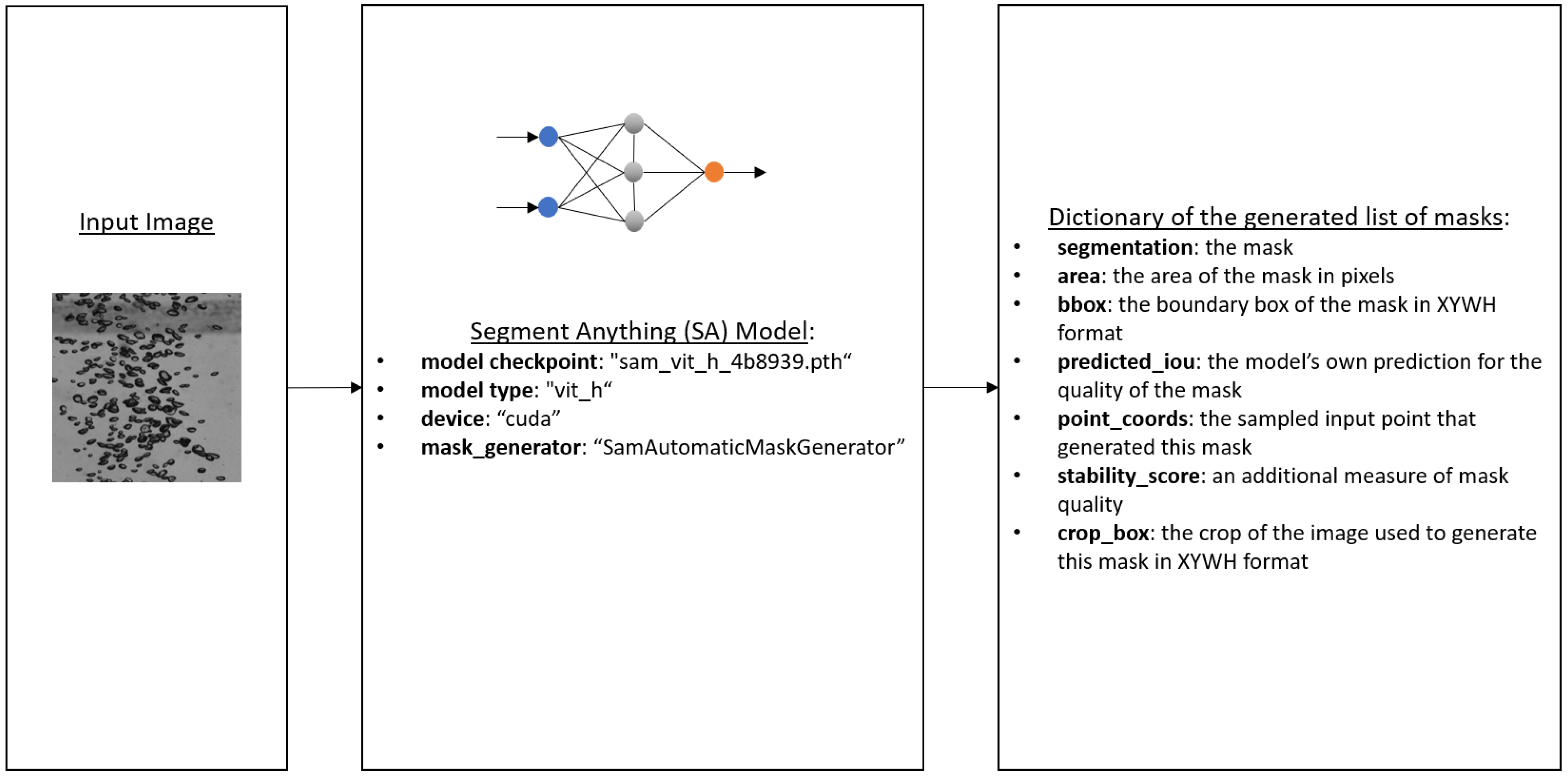
Figure 2.
The overview process scheme of creating a custom dataset for PyTorch YOLOv5 for instance segmentation.
Figure 2.
The overview process scheme of creating a custom dataset for PyTorch YOLOv5 for instance segmentation.
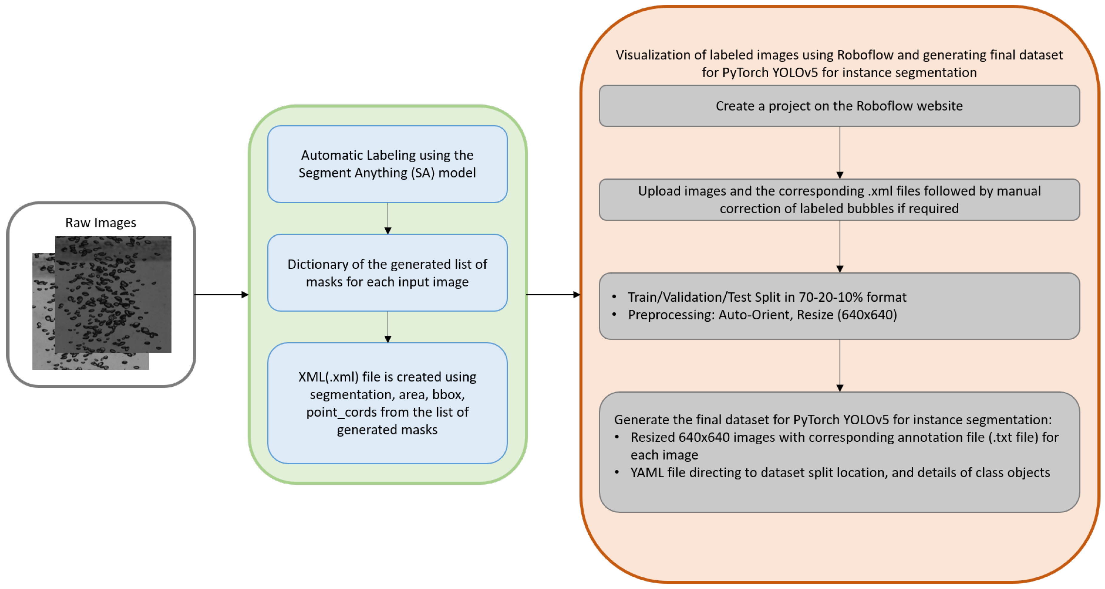
Figure 3.
A simple overview of a YOLOv5 architecture [20].
Figure 3.
A simple overview of a YOLOv5 architecture [20].
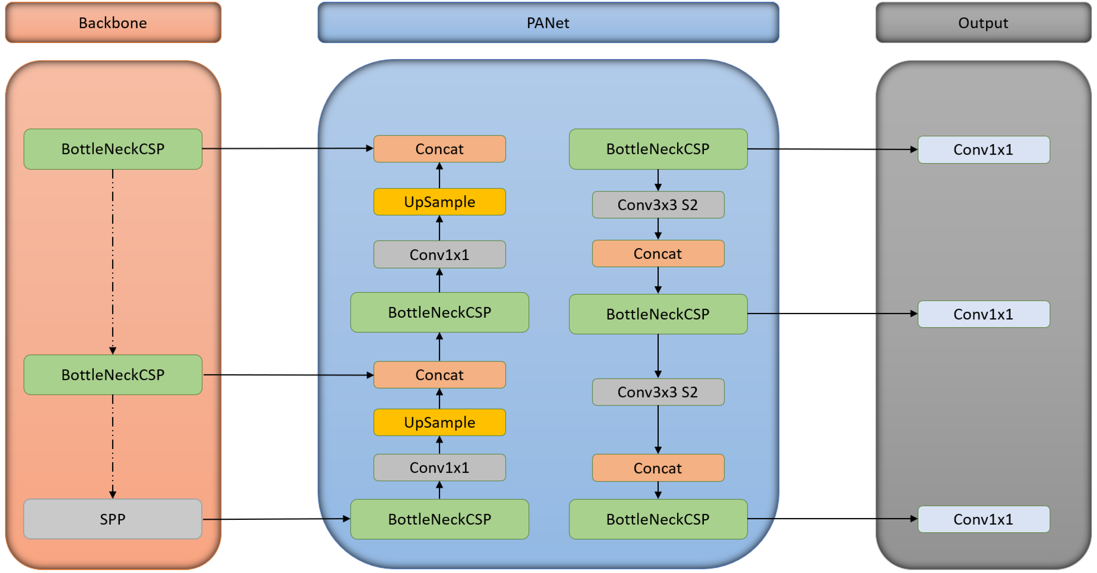
Figure 4.
A simple overview of computing IoU in object detection using ground truth and prediction bounding box.
Figure 4.
A simple overview of computing IoU in object detection using ground truth and prediction bounding box.
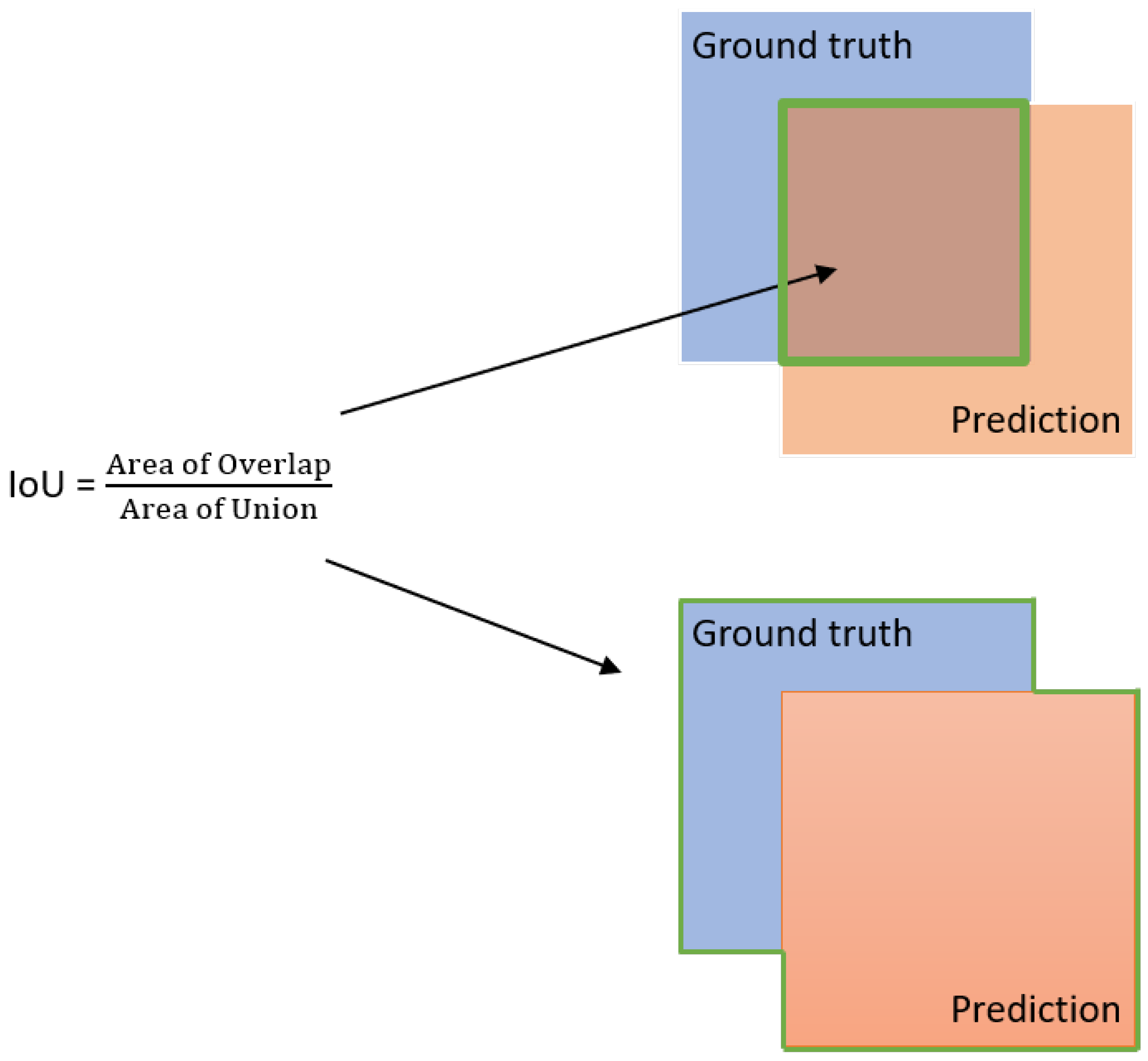
Figure 5.
A visual representation of the Confusion Matrix.
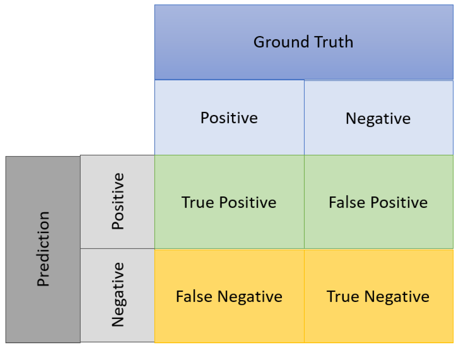
Figure 6.
Visual representation of mechanism used in YOLOv5 to eliminate grid sensitivity [20].
Figure 6.
Visual representation of mechanism used in YOLOv5 to eliminate grid sensitivity [20].
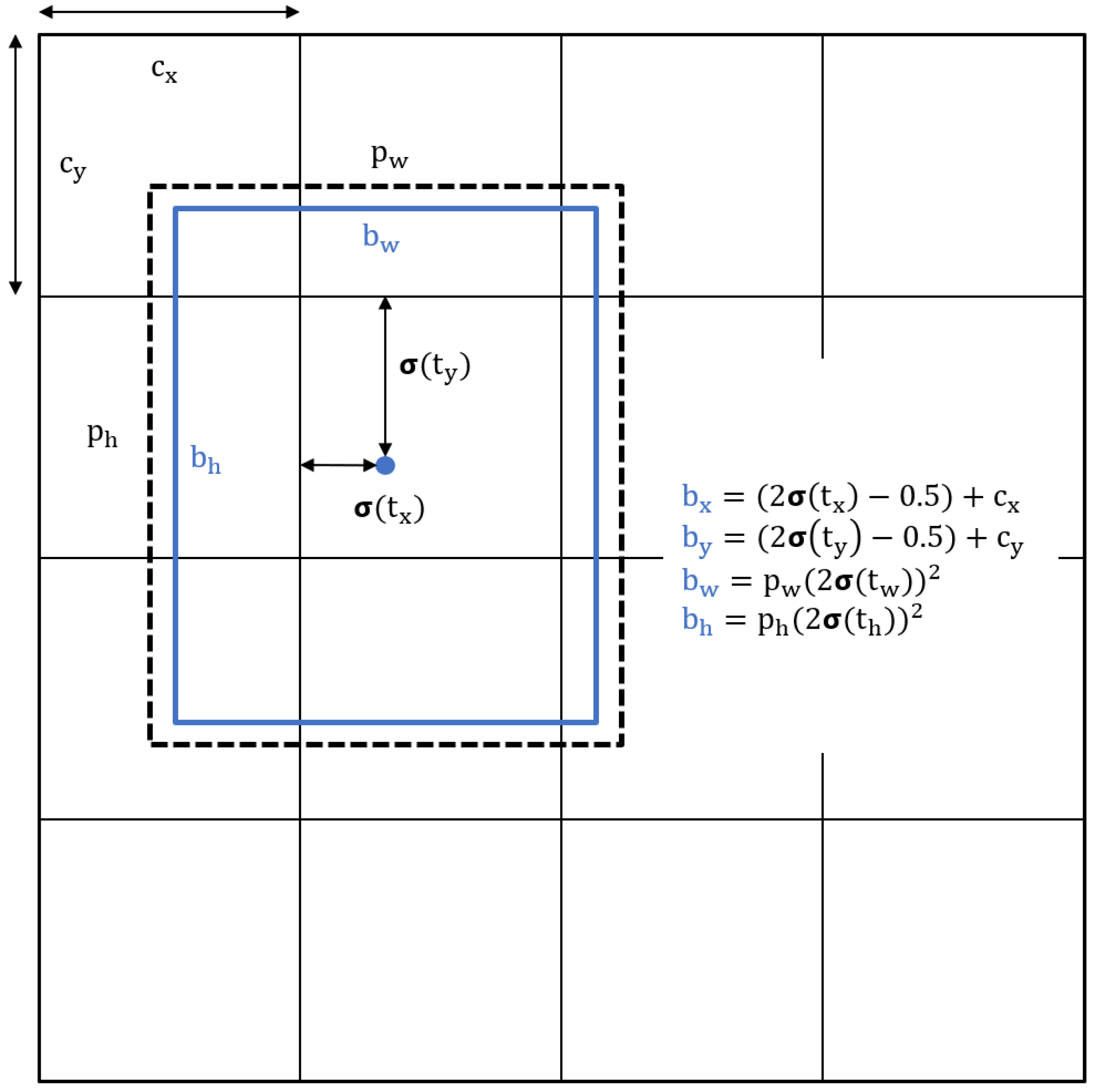
Figure 7.
A visual representation of the workflow for selecting the best-trained YOLOv5 model for the bubble dataset.
Figure 7.
A visual representation of the workflow for selecting the best-trained YOLOv5 model for the bubble dataset.
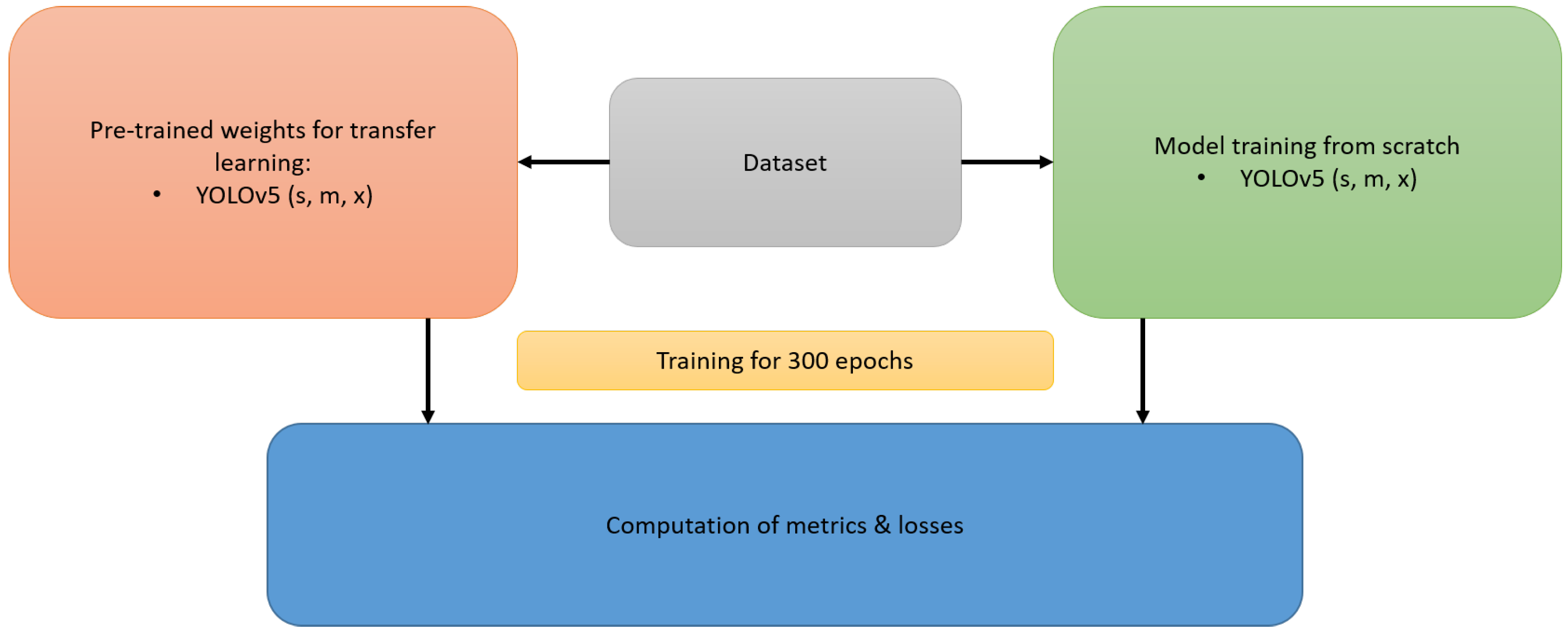
Figure 8.
YOLOv5 model training result, the above figure shows the qualitative results for training and validation losses (Y-axis) for the YOLOv5 (s, m, x) pre-trained models for 300 epochs (X-axis), during training all three models achieved the best training results before 300 epochs.
Figure 8.
YOLOv5 model training result, the above figure shows the qualitative results for training and validation losses (Y-axis) for the YOLOv5 (s, m, x) pre-trained models for 300 epochs (X-axis), during training all three models achieved the best training results before 300 epochs.
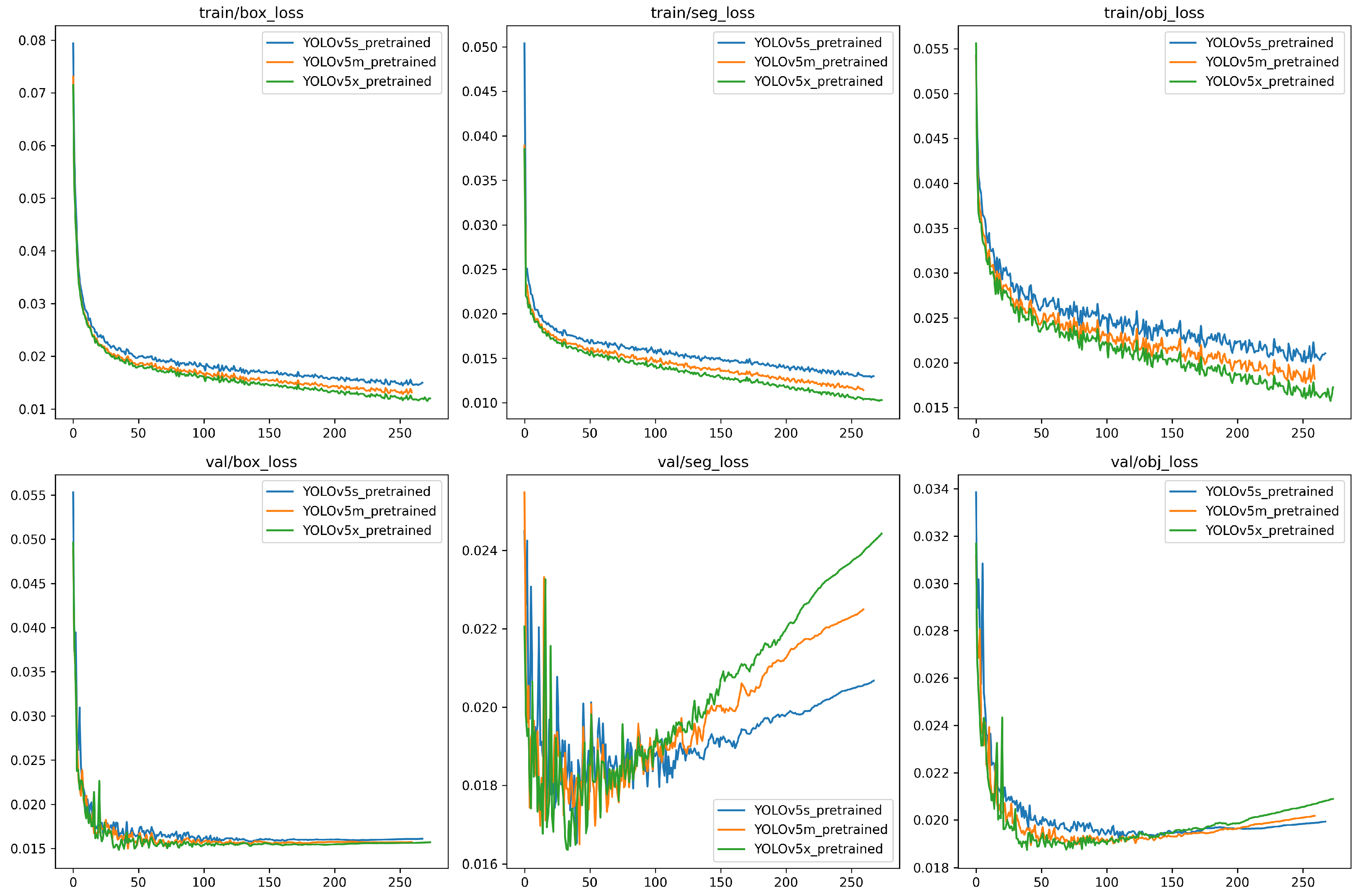
Figure 9.
A graphical representation of the YOLOv5 model evaluation on validation dataset, the figure shows the results for Precision, Recall, mAP50, and mAP50-95 (Y-axis) for both bounding box and mask for the YOLOv5 (s, m, x) models with best epoch (X-axis) respectively.
Figure 9.
A graphical representation of the YOLOv5 model evaluation on validation dataset, the figure shows the results for Precision, Recall, mAP50, and mAP50-95 (Y-axis) for both bounding box and mask for the YOLOv5 (s, m, x) models with best epoch (X-axis) respectively.
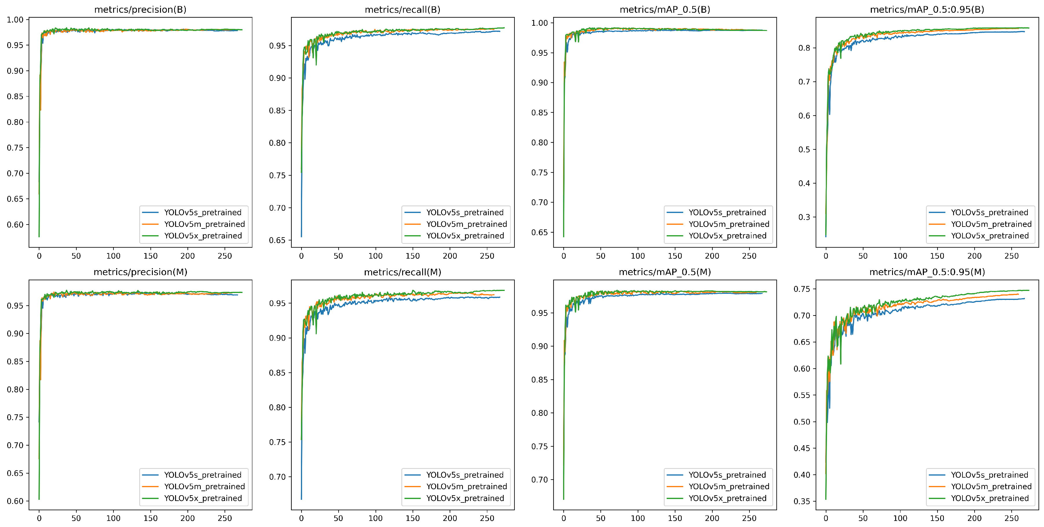
Figure 10.
This figure presents a qualitative comparison of the detection and segmentation capabilities of three YOLOv5 models (s, m, and x) on a test dataset containing images with small bubbles. The first column displays the raw images. The subsequent columns show the results obtained using YOLOv5s, YOLOv5m, and YOLOv5x, respectively.
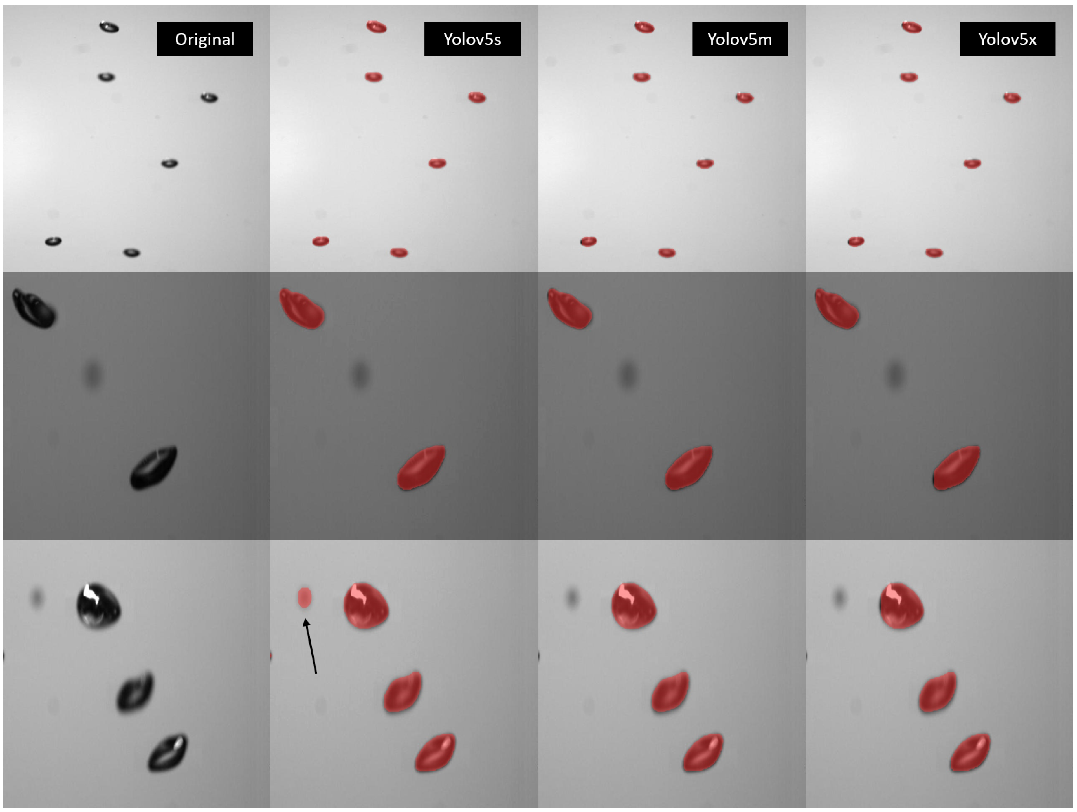
Figure 11.
This figure presents a qualitative comparison of the detection and segmentation capabilities of YOLOv5 models (s, m, and x) on the test dataset containing images with medium bubbles. The first column displays the raw images. The subsequent columns show the results obtained using YOLOv5s, YOLOv5m, and YOLOv5x, respectively.
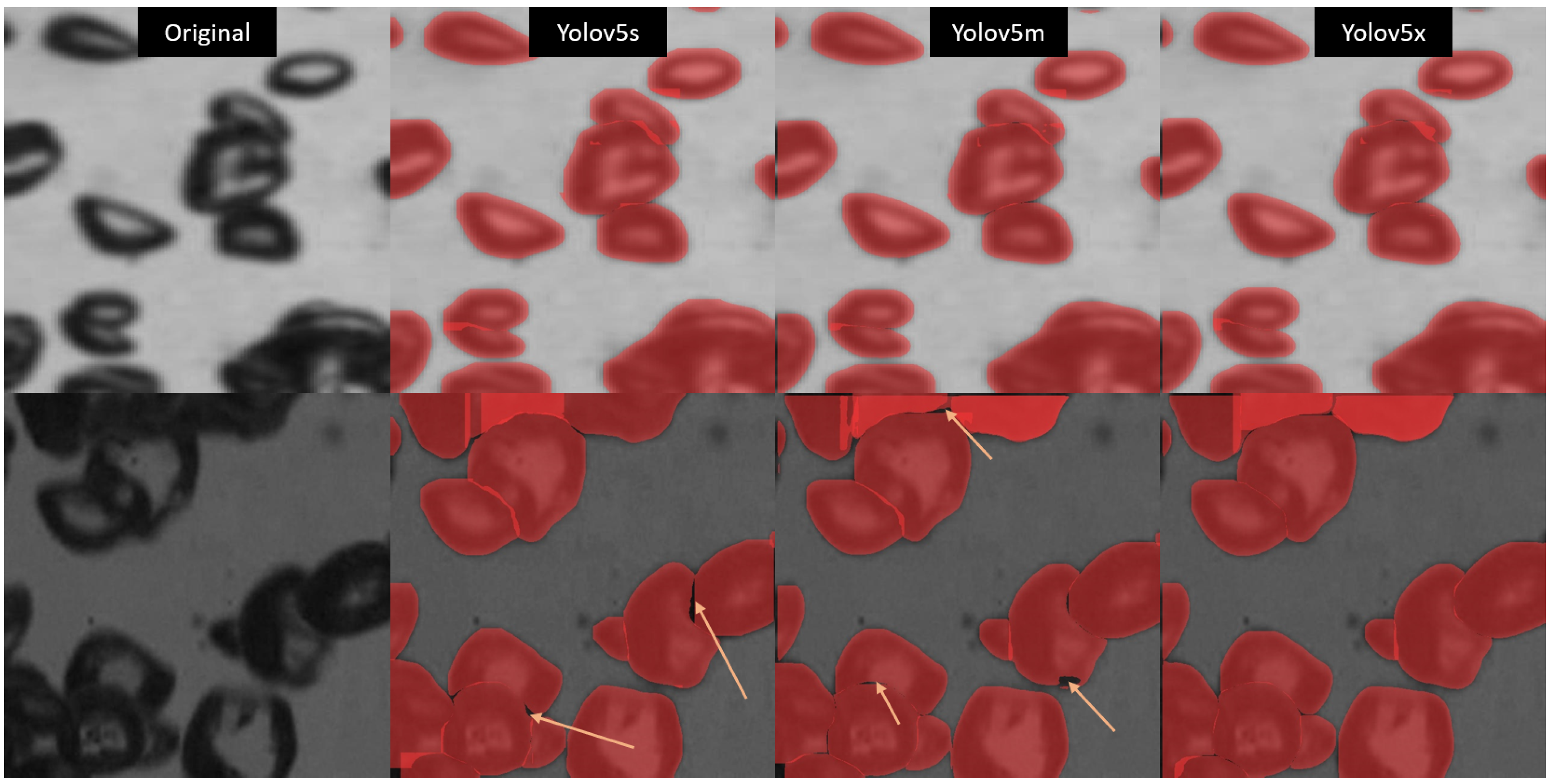
Figure 12.
This figure presents a qualitative comparison of the detection and segmentation capabilities of YOLOv5 models (s, m, and x) on the test dataset containing images with large bubbles. The first column displays the raw images. The subsequent columns show the results obtained using YOLOv5s, YOLOv5m, and YOLOv5x, respectively.
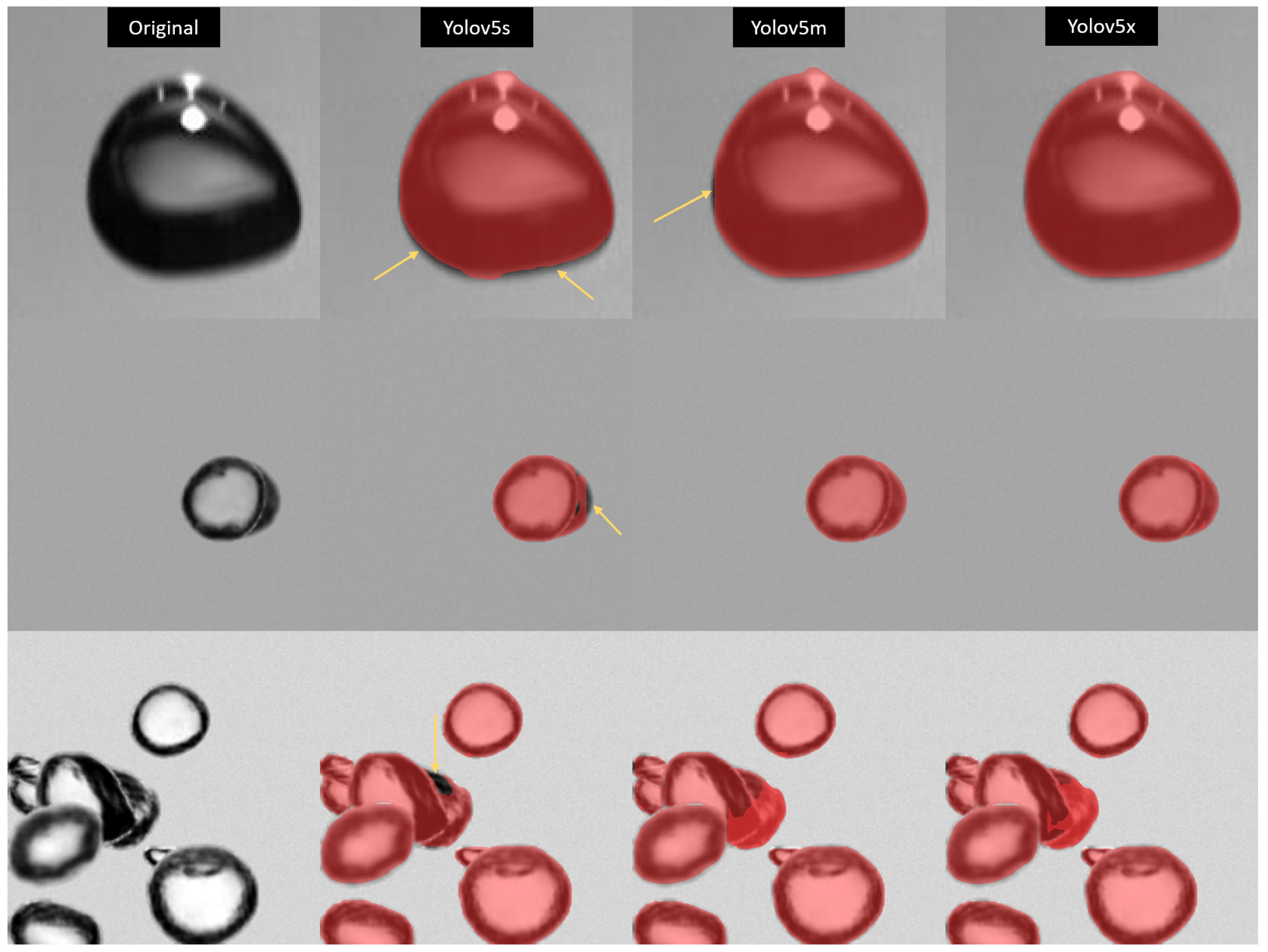
Figure 13.
Performance comparison of YOLOv5 models (s, m, x) for bubble detection and segmentation in a swarm scenario. Top-left: Raw Image. Remaining: Results from YOLOv5s (top-right), YOLOv5m (bottom-left), and YOLOv5x (bottom-right).
Figure 13.
Performance comparison of YOLOv5 models (s, m, x) for bubble detection and segmentation in a swarm scenario. Top-left: Raw Image. Remaining: Results from YOLOv5s (top-right), YOLOv5m (bottom-left), and YOLOv5x (bottom-right).
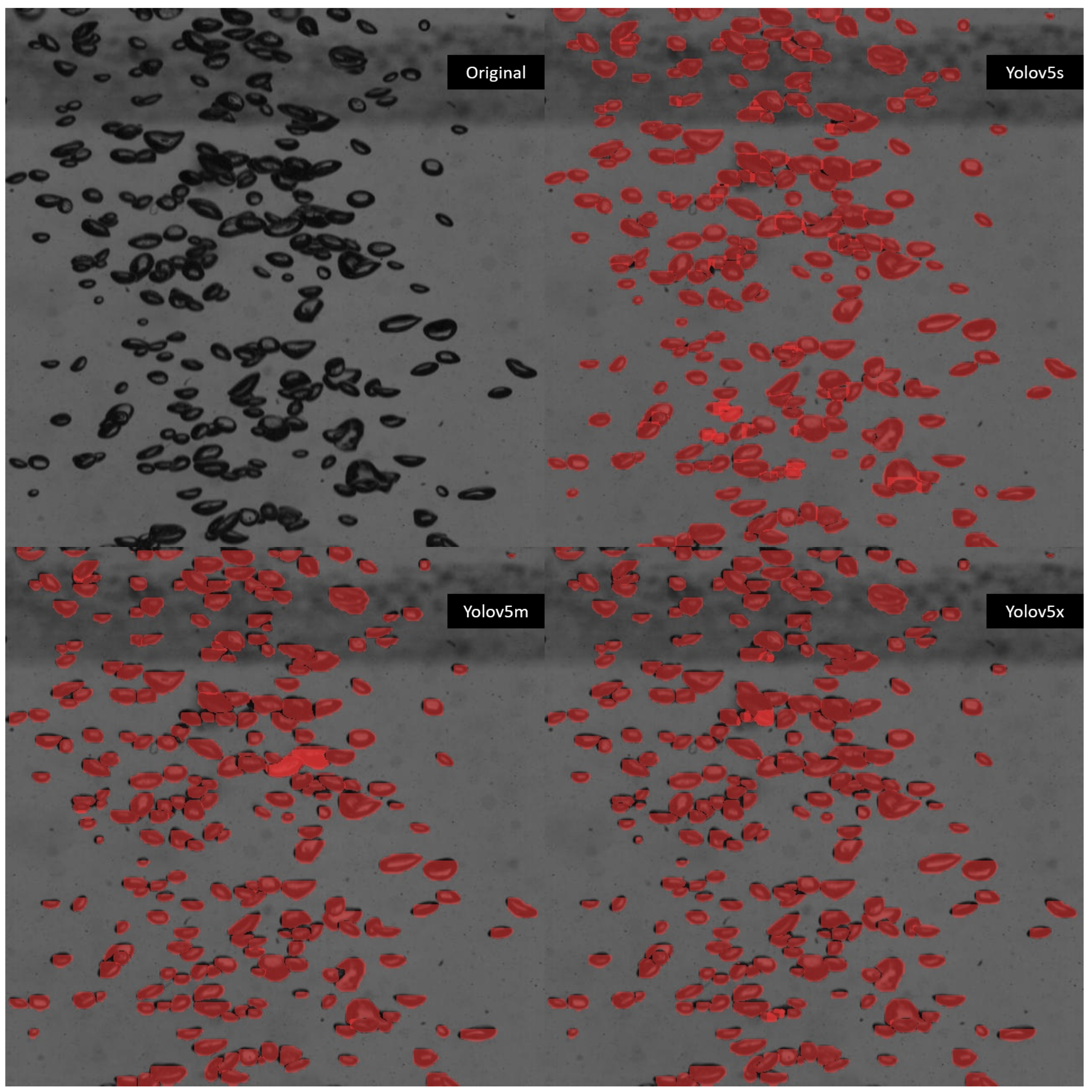
Table 1.
Performance overview of YOLOv5 segmentation models on the COCO dataset for 300 epochs using A100 GPUs [20].
Table 1.
Performance overview of YOLOv5 segmentation models on the COCO dataset for 300 epochs using A100 GPUs [20].
| Model | size (pixels) |
mAP50-95 (box) |
mAP50-95 (mask) |
Train 300 epochs (hours) |
Speed ONNX CPU (ms) |
Speed TRT A100 (ms) |
Params (M) |
FLOPs @ 640 (B) |
|---|---|---|---|---|---|---|---|---|
| YOLOv5n-seg | 640 | 27.6 | 23.4 | 80:17 | 62.7 | 1.2 | 2.0 | 7.1 |
| YOLOv5s-seg | 640 | 37.6 | 31.7 | 88:16 | 173.3 | 1.4 | 7.6 | 26.4 |
| YOLOv5m-seg | 640 | 45 | 37.1 | 108:36 | 427.0 | 2.2 | 47.9 | 147.7 |
| YOLOv5l-seg | 640 | 49 | 39.9 | 66:43 (2x) | 857.4 | 2.9 | 47.9 | 147.7 |
| YOLOv5x-seg | 640 | 50 | 41.4 | 62:56 (3x) | 1579.2 | 4.5 | 88.8 | 265.7 |
Table 2.
Model summary for YOLOv5 (s, m, x) pre-trained models, the table provides details about the important model training process and summary specifications.
Table 2.
Model summary for YOLOv5 (s, m, x) pre-trained models, the table provides details about the important model training process and summary specifications.
| Model | Best Epoch | Time (hours) | Layers | Parameters (M) | GFLOPs |
|---|---|---|---|---|---|
| YOLOv5s-seg.pt | 264 | 7.65 | 165 | 7.39 | 25.7 |
| YOLOv5m-seg.pt | 258 | 10.11 | 220 | 21.65 | 69.8 |
| YOLOv5x-seg.pt | 271 | 17.88 | 330 | 88.24 | 264 |
Table 3.
YOLOv5 model evaluation on validation dataset, the table shows the quantitative results for Precision, Recall, mAP50, and mAP50-95 for both bounding box and mask for the YOLOv5 (s, m, x) models.
Table 3.
YOLOv5 model evaluation on validation dataset, the table shows the quantitative results for Precision, Recall, mAP50, and mAP50-95 for both bounding box and mask for the YOLOv5 (s, m, x) models.
| Model | Box | Mask | ||||||
|---|---|---|---|---|---|---|---|---|
| Precision | Recall | mAP50 | mAP50-95 | Precision | Recall | mAP50 | mAP50-95 | |
| YOLOv5s-seg.pt | 0.978 | 0.972 | 0.987 | 0.848 | 0.969 | 0.958 | 0.979 | 0.731 |
| YOLOv5m-seg.pt | 0.98 | 0.975 | 0.988 | 0.857 | 0.973 | 0.962 | 0.981 | 0.74 |
| YOLOv5x-seg.pt | 0.98 | 0.977 | 0.987 | 0.859 | 0.974 | 0.969 | 0.982 | 0.747 |
Table 4.
YOLOv5 model evaluation on the test dataset, the table shows the quantitative results for Precision, Recall, mAP50, and mAP50-95 for both bounding box and mask for the YOLOv5 (s, m, x) models.
Table 4.
YOLOv5 model evaluation on the test dataset, the table shows the quantitative results for Precision, Recall, mAP50, and mAP50-95 for both bounding box and mask for the YOLOv5 (s, m, x) models.
| Model | Box | Mask | ||||||
|---|---|---|---|---|---|---|---|---|
| Precision | Recall | mAP50 | mAP50-95 | Precision | Recall | mAP50 | mAP50-95 | |
| YOLOv5s-seg.pt | 0.986 | 0.973 | 0.988 | 0.848 | 0.976 | 0.962 | 0.98 | 0.738 |
| YOLOv5m-seg.pt | 0.987 | 0.977 | 0.989 | 0.856 | 0.977 | 0.963 | 0.982 | 0.742 |
| YOLOv5x-seg.pt | 0.986 | 0.979 | 0.989 | 0.856 | 0.978 | 0.967 | 0.982 | 0.743 |
Disclaimer/Publisher’s Note: The statements, opinions and data contained in all publications are solely those of the individual author(s) and contributor(s) and not of MDPI and/or the editor(s). MDPI and/or the editor(s) disclaim responsibility for any injury to people or property resulting from any ideas, methods, instructions or products referred to in the content. |
© 2024 by the authors. Licensee MDPI, Basel, Switzerland. This article is an open access article distributed under the terms and conditions of the Creative Commons Attribution (CC BY) license (https://creativecommons.org/licenses/by/4.0/).
Copyright: This open access article is published under a Creative Commons CC BY 4.0 license, which permit the free download, distribution, and reuse, provided that the author and preprint are cited in any reuse.


