
Submitted:
15 April 2026
Posted:
15 April 2026
You are already at the latest version
Abstract
We define the function $Col: \mathbb{N} \to \mathbb{N}$ as the Collatz function, given by \(3n + 1\) if \(n\) is odd and \(\displaystyle\frac{n}{2}\) if \(n\) is even. The conjecture postulates that for any positive integer, at some point, its iteration will reach 1, or equivalently, every orbit will fall into the periodic cycle $\{4, 2, 1\}$. Two conditions would invalidate the conjecture: The existence of a divergent orbit or the presence of another cycle. We can study the dynamics of the orbits through the density of even terms in their orbit. If all points' accumulation density exceeds the value of \(\displaystyle\frac{\ln(3)}{\ln(2)}\) then the orbit is bounded. The main result of this work is to show that there are no natural numbers such that the accumulation points of the pair density are less than \(\displaystyle\frac{\ln(3)}{\ln(2)}\). In other words, there are no divergent orbits.
Keywords:
Collatz conjecture
; dynamical system
| Contents | ||
| 1 | Collatz’s Conjecture | 1 |
| 1.1 Main Idea of This Work.................................................................................................................................................. | 1 | |
| 1.2 Notations and Conventions............................................................................................................................................... | 1 | |
| 1.3 Organization of the Paper............................................................................................................................................... | 1 | |
| 2 | Background | 1 |
| 2.1 Metric Space............................................................................................................................................................ | 1 | |
| 2.2 Limit Superior (lim sup) and Limit Inferior (lim inf) of a Sequence:.................................................................................................... | 1 | |
| 2.3 Number Theory........................................................................................................................................................... | 1 | |
| 2.4 The Baker–Wüstholz Theorem on Linear Forms in Logarithms (Rational Case)............................................................................................. | 1 | |
| 2.5 The Ring of 2-Adic Integers Z2......................................................................................................................................... | 1 | |
| 2.6 Dynamical System........................................................................................................................................................ | 1 | |
| 3 | Set Generate by θ and ψq | 1 |
| 3.1 Summary of Propositions in the Section.................................................................................................................................. | 1 | |
| 3.2 Set Generate by θ and ψq.............................................................................................................................................. | 1 | |
| 4 | Stability and Instability of Integer Set | 1 |
| 4.1 Summary of Propositions in the Section.................................................................................................................................. | 1 | |
| 4.2 Stability and Instability of Integer Set................................................................................................................................ | 1 | |
| 5 | Coding of the Orbits | 1 |
| 5.1 Summary of Propositions in the Section.................................................................................................................................. | 1 | |
| 5.2 Coding of the Orbits.................................................................................................................................................... | 1 | |
| 5.3 Extension of the Collatz function on Q.................................................................................................................................. | 1 | |
| 6 | The G0, G∞ and G1 Sets | 1 |
| 6.1 Summary of Propositions in the Section.................................................................................................................................. | 1 | |
| 6.2 The G0, G∞, and G1 Sets............................................................................................................................................... | 1 | |
| 7 | Extension of the Collatz Function to Z2 | 1 |
| 7.1 Summary of Propositions in the Section.................................................................................................................................. | 1 | |
| 7.2 Extension of the Collatz Function to Z2................................................................................................................................. | 1 | |
| 7.3 Topological Conjugation................................................................................................................................................. | 1 | |
| 7.4 Periodic Points Analysis................................................................................................................................................ | 1 | |
| 8 | Real Function π1 and π2 Function | 1 |
| 8.1 Summary of Propositions in the Section.................................................................................................................................. | 1 | |
| 8.2 The π1 and π2 Functions............................................................................................................................................... | 1 | |
| 8.3 Definitions............................................................................................................................................................. | 1 | |
| 8.4 Characterization of G0 and G∞......................................................................................................................................... | 1 | |
| 9 | The Sigma Function | 1 |
| 9.1 Summary of Propositions in the Section.................................................................................................................................. | 1 | |
| 9.2 The Sigma Function...................................................................................................................................................... | 1 | |
| 9.3 Properties of the Sigma Function........................................................................................................................................ | 1 | |
| 9.4 The Sigma Function Modulo a............................................................................................................................................. | 1 | |
| 9.5 Extension of the Sigma Function to Qodd................................................................................................................................. | 1 | |
| 9.6 Properties of the Extension of the Sigma Function....................................................................................................................... | 1 | |
| 9.7 Coding of Sigma Function................................................................................................................................................ | 1 | |
| 10 | Coding of Set G∞ | 1 |
| 10.1 Summary of Propositions in the Section.................................................................................................................................. | 1 | |
| 10.2 π1(G∞) as Complete Metric Space...................................................................................................................................... | 1 | |
| 10.3 Topological Conjugation................................................................................................................................................. | 1 | |
| 11 | The G1 Is Positive Unstable | 1 |
| 11.1 Summary of Propositions in the Section.................................................................................................................................. | 1 | |
| 11.2 The Fix Function........................................................................................................................................................ | 1 | |
| 11.3 Minimality.............................................................................................................................................................. | 1 | |
| 11.4 G1 Is Unstable.......................................................................................................................................................... | 1 | |
| 12 | The Problem of Divergence | 1 |
| 12.1 Summary of Propositions in the Section.................................................................................................................................. | 1 | |
| 12.2 The Problem of Divergence............................................................................................................................................... | 1 | |
| 13 | Conclusion | 1 |
| References | 1 | |
1. Collatz’s Conjecture
The Collatz conjecture, also known as the conjecture, is an unsolved problem in number theory proposed by the German mathematician Lothar Collatz in 1937. Despite its seemingly simple formulation, it has challenged mathematicians for decades due to the extreme difficulty of proving its validity or finding a counterexample.
The formal formulation of the conjecture is as follows:
Let be defined by:
Then, for all , there exists such that:
An equivalent formulation of the conjecture argues that starting from any positive integer, the sequence will eventually reach the cycle . Two scenarios could invalidate the conjecture: the existence of a cycle strictly different from , or the existence of a divergent orbit (an orbit that grows toward infinity). To date, no evidence has been found for either of these exceptions; however, no rigorous proof has completely ruled them out. In 2019, Terence Tao [16] presented a major breakthrough demonstrating that almost all orbits attain almost bounded values (falling very close to the cycle).
Example 1.
Example 2.
1.1. Main Idea of This Work
The primary contribution of this work is not simply a proof concerning the Collatz Conjecture, but the development of a comprehensive mathematical framework: the Theory of Infinite Systems of Linear Diophantine Equations. For decades, the Collatz problem has resisted traditional approaches because its discrete dynamics are highly chaotic. To conquer this, our central premise establishes that the existence of divergent orbits must be translated into a rigid algebraic structure. Specifically, a divergent orbit can only exist if there is a simultaneous natural solution to an endlessly growing, infinitely constrained system of linear Diophantine equations.
To navigate and eventually break this infinite system, the majority of this paper is dedicated to building the necessary theoretical machinery from the ground up. We do this in three fundamental steps:
1. Construction of the Diophantine System: We associate to each natural number a unique binary sequence that represents the parity of its iterations. Every finite truncation of this sequence generates a specific affine linear transformation, which in turn defines a linear Diophantine equation. A divergent orbit would require a single natural number to perfectly satisfy this endless sequence of equations.
2. The Sigma Function () as the Analytical Engine: A critical challenge in this infinite system is tracking the ever-shifting constants generated by the affine transformations. To solve this, we introduce the Sigma function (). Far from being a mere auxiliary calculation, the Sigma function is the core algebraic tool of our theory. It exactly parametrizes and tracks the minimal non-negative solutions () of these Diophantine equations across infinite iterations, allowing us to measure the precise "friction" between multiplications and divisions.
3. Topological Classification and the Critical Threshold: To evaluate whether a simultaneous solution can exist, the sequence is encoded by assigning 0 if the iteration is even, and 10 if it is odd. We define the density function as the ratio , where is the total number of 0’s up to the k-th occurrence of the digit 1.
The critical threshold arises naturally from the geometric growth of the Collatz operations. An odd step multiplies the value by roughly 3, while an even step divides it by 2. After k odd steps and even steps, the global magnitude of the orbit is scaled by a factor of approximately . Setting this overall growth factor to 1 to find the state of equilibrium yields . By taking the natural logarithm, we obtain the precise ratio . Thus, this constant represents the exact arithmetic break-even point between the expansion and contraction of the orbit.
Using this threshold, our theory classifies all infinite sequences into three distinct sets:
- : The set of sequences where . Here, divisions by 2 strictly dominate. We prove that any integer whose coding falls into must inevitably have a bounded orbit.
- : The set of sequences where . Here, multiplications by 3 dominate. We prove that no natural number can exist in , because the “real-valued” limits of such sequences strictly map to negative integers or rationals.
- : The exact boundary where . This is the critical equilibrium threshold. By bridging our Diophantine theory with bounds from transcendental number theory, we demonstrate that this delicate balance is positively unstable. It cannot contain the coding of any natural number without the orbit exploding in a mathematically contradictory way.
Once this theoretical framework is fully established, the resolution of the Collatz divergence problem emerges as a natural, unavoidable consequence. Formally, we establish the following foundational results:
- 1.
- There is no whose coding satisfies .
- 2.
- The coding of belongs to if and only if its orbit is bounded.
We leverage this machinery to demonstrate the main theorem of this work:
Theorem 12:
There are no divergent orbits for the Collatz function on the natural numbers.
The core idea of the final proof is by contradiction: Suppose there exists an whose orbit is divergent. Then, necessarily, its coding cannot belong to . This means there must exist a subsequence of its density function whose limit is less than or equal to . Moreover, the density function cannot have accumulation points strictly greater than , because otherwise, there would exist a sub-orbit of n that is bounded (a consequence of Corollary 2).
Trapped by these restrictions, all accumulation points of the density function must be strictly less than or equal to . However, our established theory proves that contains no natural numbers, and the equilibrium in is positively unstable. Hence, the encoding of a divergent natural number has absolutely no valid mathematical space to exist within the topology of , making divergent orbits an impossibility.
1.2. Notations and Conventions
In this work, we denote the set of positive integers as , the set of non-negative integers as , the greatest common divisor of a and b as , and the least common multiple of a and b as .
We use the following symbology to refer to an arbitrary composition of functions:
1.3. Organization of the Paper
Due to the multidisciplinary nature of the mathematical tools employed, this work is structurally divided into three distinct parts. This division guides the reader from discrete arithmetic to continuous topological analysis, culminating in the resolution of the conjecture’s main problems.
Part I: Elementary Theory of Infinite Systems of Diophantine Equations (Chapters 1–5)
This first part establishes the discrete and algebraic framework of the problem, transforming dynamic orbits into coded sequences and systems of linear equations.
Main Definitions:
- Binary Coding of the Orbits (): The rule that translates the trajectory of a number into a symbolic sequence, assigning 0 for even steps and 10 for odd steps.
- Local Affine Transformations (): The representation of each finite truncation of the coded sequence as a linear affine map of the form .
- Stability of Integer Sets: The discrete criteria defining how the set of valid integer solutions evolves and is restricted as more iterations are added to the system.
Main Results:
- Diophantine Equivalence: It is demonstrated that the existence of any Collatz orbit is strictly equivalent to the existence of a simultaneous integer solution for an infinite system of Diophantine equations of the form .
- We prove that by composing the affine functions, the sets of integer solutions are strictly nested within each other ().
Chapters Overview:
- Chapter 1 & 2 (Collatz’s Conjecture & Background): Introduce the problem, the scenarios that would invalidate the conjecture, and the fundamental mathematical tools (metric spaces, p-adic analysis, Diophantine equations).
- Chapter 3 (Set Generated by and ): Models the Collatz operations as affine transformations and formalizes the integer sets generated by their truncations.
- Chapter 4 (Stability and Instability of Integer Sets): Establishes the algebraic rules governing the bounds of the integer solution sets.
- Chapter 5 (Coding of the Orbits): Details the symbolic binary assignment and explores the extension of the Collatz function over the odd rationals ().
Part II: Analytic Theory of Infinite Systems of Diophantine Equations (Chapters 6–11)
Here, the research takes a qualitative leap: the discrete problem is translated into the calculus of limits, 2-adic topology, and linear forms in logarithms.
Main Definitions:
- Parity Density Function: The asymptotic ratio , which measures the proportion between divisions by 2 and multiplications by 3.
- The Topological Sets (): The partition of all possible codings based on the critical threshold . represents division-dominated orbits, multiplication-dominated ones, and the perfect equilibrium.
- The 2-adic Space () and Functions: The extension of the domain to treat infinite sequences as convergent real series.
- The Sigma Function (): A fundamental auxiliary function introduced to trace the evolution of the constants in the Diophantine system.
Main Results:
- Exact Parameterization (Theorem 6): It is proved that the iterations of the Sigma Function exactly construct the minimal non-negative solution () of any generated Diophantine equation.
- Invariance of : We demonstrate topologically that any sequence dominated by multiplications by 3 corresponds strictly to negative integers or rational numbers, never to a natural number.
- The Positive Instability of : By invoking the Baker-Wüstholz Theorem (bounds for linear forms in logarithms), we prove that the delicate equilibrium at the threshold is positively unstable. The transcendental bound forces an infinite accumulation of binary carries, destroying the possibility of an integer solution.
Chapters Overview:
- Chapter 6 (The and Sets): Divides the total space of coding sequences based on their asymptotic density limits.
- Chapter 7 & 8 ( Extension & Real Functions ): Translates the system’s domain to the 2-adic integers and constructs weight functions to map topological evolution to real values.
- Chapter 9 (The Sigma Function): Introduces the main algebraic tool used to find minimal solutions for the affine mappings.
- Chapter 10 (Coding of Set ): Topologically proves that natural numbers cannot exhibit multiplication-dominated behavior.
- Chapter 11 (The Set is Unstable): The climax of the analytic theory, where transcendental number theory is applied to break the critical threshold.
Part III: The Proof of the Non-Existence of Divergent Orbits (Chapter 12)
The resolution section of the paper. All the analytic machinery developed in Parts I and II is directly applied to prove that divergent trajectories are mathematically impossible.
Main Definitions:
- Divergent Orbits: Trajectories generated by the Collatz function over the natural numbers that escape to infinity, i.e., .
Main Results:
- Non-Existence of Divergent Orbits (Main Theorem): We formally conclude that, since the codings of natural numbers cannot belong to or (as proven by the topological and transcendental bounds of Part II), every natural number strictly belongs to the set . This mathematically guarantees that the density of divisions by 2 eventually strictly dominates the multiplications by 3, implying that every orbit is bounded and no divergent orbits can exist.
Chapters Overview:
- Chapter 12 (The Problem of Divergence): Consolidates the theorems from the analytic theory to definitively prove that no natural number can have a divergent trajectory, successfully ruling out this major scenario for the Collatz Conjecture.
2. Background
2.1. Metric Space
A metric space is a set X equipped with a function , called a metric, that satisfies the following properties for all :
- Non-negativity:, and if and only if .
- Symmetry:.
- Triangle inequality:.
The function measures the "distance" between any two points x and y in the set X. The pair is called a metric space.
Examples of Metrics:
-
Euclidean Metric (on ):This metric defines the usual distance between two points and in Euclidean space .
-
Discrete Metric:In this metric, the distance between two distinct points is always 1, and the distance from any point to itself is 0.
-
Taxicab Metric (or Manhattan Metric, on ):This metric measures the distance between two points x and y as the sum of the absolute differences of their coordinates. It corresponds to the distance a taxi would drive on a grid of city streets.
-
p-adic Metric (on ):Here, p is a fixed prime number, and denotes the p-adic valuation of , whichThis metric measures the distance between two rational numbers based on their divisibility by p. The p-adic metric induces a non-Archimedean topology, meaning that the "triangle inequality" is strengthened to .
A complete metric space is a metric space in which every Cauchy sequence converges to a point within the space. Formally, a metric space is called complete if, for every sequence that is Cauchy (i.e., for any , there exists such that for all , ), there exists a point such that:
In other words, all Cauchy sequences in X must have a limit in X.
Examples:
- The Real Numbers with the Euclidean Metric: The set of real numbers with the usual Euclidean metric is a complete metric space. This is because every Cauchy sequence of real numbers converges to a real number.
- The Rational Numbers with the Euclidean Metric: The set of rational numbers with the Euclidean metric is not complete. For example, the sequence defined by and that approximate is Cauchy in but does not converge to a rational number (since ).
- The p-adic Numbers : The set of p-adic numbers , equipped with the p-adic metric , is a complete metric space. Every Cauchy sequence in converges to a p-adic number within .
2.2. Limit Superior (lim sup) and Limit Inferior (lim inf) of a Sequence:
Given a sequence of real numbers and . Let us consider the following subsequences of given by
we have that the sequence is monotonically increasing and is monotonically decreasing, that is:
Therefore there are limits
We will write and and we will call Limit Inferior and Limit Superior respectively.
Limit Superior (lim sup) and Limit Inferior (lim inf) of a Sequence of Sets: Let be a sequence of sets in a space X. The limit superior and limit inferior of the sequence of sets are defined as follows:
- 1.
- Set Sequence limit superior ():
- 2.
- Set Sequence limit inferior ():
- 3.
-
Limit of a Sequence of Sets If , then the sequence converges, and its limit is denoted as:Particular Case: Monotone Sequences of SetsNon-Decreasing Sequence (): If is a non-decreasing sequence (i.e., for all n), then:In this case, the limit of the sequence is simply the union of all the sets in the sequence. Non-Increasing Sequence (): If is a non-increasing sequence (i.e., for all n), then:In this case, the limit of the sequence is simply the intersection of all the sets in the sequence.
2.3. Number Theory
A linear Diophantine equation is an equation of the form
where . Such an equation has integer solutions if and only if the greatest common divisor divides c. When solutions exist, they form an infinite family given by:
where is a particular solution.
The Carmichael function is defined for each integer as the smallest positive integer m such that
for every integer a with . That is, is the exponent of the multiplicative group of units modulo n.
Some properties of include:
- If n is a power of an odd prime, say with p odd and , then .
- If , then:
- If n has the prime power decomposition , then:
2.4. The Baker–Wüstholz Theorem on Linear Forms in Logarithms (Rational Case)
In this subsection we present a simplified and completely elementary version of the main theorem of Baker and Wüstholz (1993), restricted exclusively to the case where the numbers are rational, distinct from zero and one. In this way, any reference to algebraic number fields of degree greater than 1 is avoided.
Let be a nonzero rational number, written in irreducible form as with , and . The logarithmic height of is defined by
The associated modified height is
Theorem 1:
(Baker–Wüstholz, 1993 – rational version). Let be rational numbers, none zero or one. Consider the linear form
with integer coefficients , not all zero. If
and then
where
and
Particular case: with not both zero and . Take , , and the linear form . Let .
Then:
- 1.
- 2.
- (since )
- 3.
Then
or equivalently
2.5. The Ring of 2-Adic Integers
To establish a rigorous algebraic foundation for the subsequent analysis, we must introduce the ring of 2-adic integers and its topological properties. This provides the necessary framework to study sequences and limits within a context where the standard Euclidean metric is replaced by one based on divisibility by 2.
Definition 1
(2-adic Valuation and Norm). For any non-zero rational number , we can uniquely write it in the form , where and ν are integers, and both p and q are odd. We define the2-adic valuationas . Conventionally, we set .
The2-adic normis defined as:
This norm induces an ultrametric given by .
Definition 2
(2-adic Integers). The ring of 2-adic integers, denoted as , is the metric completion of the set of integers with respect to the norm . Every element admits a unique canonical representation as an infinite power series:
The sequence of coefficients is known as the 2-adic expansion of α.
Lemma 1.
A rational number (in simplest form) belongs to if and only if its denominator q is odd.
Proof.
Let with . The rational number r belongs to if and only if , which is equivalent to . By definition, . Since p and q are coprime, they cannot both be even. If q is even, then and , leading to , meaning . If q is odd, then , so , and thus . □
The following theorem is fundamental for characterizing rational numbers within the 2-adic framework.
Theorem 2:
(Eventually Periodic Expansion of Rationals). Let . The 2-adic expansion of α is eventually periodic if and only if α is a rational number.
Proof.
Suppose the 2-adic expansion of is eventually periodic. Then, we can write , where is the pre-periodic integer part (of length k) and B is the strictly periodic part with period T. We can express B as an infinite geometric series:
where P is the integer formed by the periodic block of bits. Since P and are integers, B is a rational number. Because A and are also integers, we conclude that .
Let . By Lemma 1, we know q must be odd. Without loss of generality, suppose . By Euler’s Theorem, since , there exists an integer such that . Therefore, for some integer m. Thus, we can rewrite the fraction as:
By applying classical long division, the term generates a sequence of remainders that must necessarily repeat because the divisor is constant. This induces a sequence of coefficients in the power series expansion of 2 that is eventually periodic, with a period dividing T. □
An important geometric consequence arises when considering the sign of rational numbers within their 2-adic expansion.
Lemma 2
(2-adic Expansion of Negative Numbers). Let . If (in the sense of the standard metric in ), then the 2-adic expansion of α contains an infinite number of non-zero coefficients (infinite ’1’ bits). In particular, if α is a negative integer, its expansion possesses an infinite, uninterrupted tail of ones.
Proof.
For the case of a negative integer, consider . In , we can evaluate the sum of the infinite geometric series:
Multiplying by 2, we obtain . Solving for S under 2-adic arithmetic yields . Hence, the canonical representation of is . Any other negative integer can be expressed using two’s complement arithmetic, which guarantees that the most significant digits will all be ’1’ from a certain point onward.
For the general case of a negative rational fraction (with and q odd), we know from Theorem 2 that its expansion is eventually periodic. Assume for the sake of contradiction that the expansion contains only a finite number of ones. This would imply that after some index N, all coefficients are 0. However, if a 2-adic expansion ends in an infinite tail of zeros, the infinite series is structurally just a finite sum of positive powers of 2. In , a finite sum of non-negative terms must be a non-negative integer. This strictly defines a positive integer or zero, which contradicts the initial premise that . Therefore, the periodic part of the expansion of any negative rational must contain at least one ’1’ bit, thereby ensuring that the overall expansion possesses infinitely many ’1’ bits. □
Lemma 3
(Purely Periodic Expansion of Rationals). Let . The 2-adic expansion of α is purely periodic (meaning it possesses no pre-periodic block) if and only if . In particular, it is non-trivially purely periodic if and only if .
Proof.
Suppose the 2-adic expansion of is purely periodic with a period of length . We can express as a direct infinite geometric series:
where P is the integer value formed by the periodic block of T bits. The maximum possible value for a T-bit integer occurs when all its bits are ’1’, yielding . Since , we can bound as follows:
Excluding the trivial constant sequences where (yielding ) and (yielding ), any strictly non-trivial purely periodic sequence maps to a rational number .
Conversely, let be a rational number in . By Lemma 1, with and q odd. By Euler’s Theorem, since , there exists an integer such that q divides , meaning for some integer . We can rewrite as:
Since , multiplying the inequality by m yields . Let . Because , P can be exactly represented as a positive T-bit binary integer. Expanding the fraction back into a geometric series yields:
This explicitly constructs a purely periodic 2-adic expansion for without any pre-periodic terms, completing the proof. □
2.6. Dynamical System
A discrete dynamical system is a model of the evolution of a state over discrete time steps. Formally, it consists of a set X (called the state space) and a function that describes how the state evolves from one time step to the next. The system is described by the equation:
where represents the state of the system at the n-th time step. The evolution of the system is typically studied by iterating the function, f starting from an initial state . The sequence , where , is called the orbit or trajectory of the initial state .
Topologically Conjugate Dynamical Systems: Two discrete dynamical systems and are said to be topologically conjugate if there exists a homeomorphism such that the following diagram commutes:
In other words, the systems and are topologically conjugate if there is a bijective function such that:
- h is a homeomorphism, meaning h is continuous, bijective, and its inverse is also continuous.
- The following relation holds:
This means that the dynamics of f on X and g on Y are the same up to a change of coordinates given by h. The systems and have the same qualitative behavior, such as the structure of orbits and periodic points, despite potentially differing in their specific representations.
Properties of Topological Conjugation with Respect to Orbits and Periodic Points:
- Preservation of Orbits: If and are two topologically conjugate dynamical systems, with a homeomorphism such that , then h preserves the orbits of points. Specifically, for any point , the orbit of x under f is mapped to the orbit of under g by h. Mathematically, this means:
-
Preservation of Periodic Points: If is a periodic point of f with period p, then is a periodic point of g with the same period p. Specifically, if , then:Conversely, if is a periodic point of g with period p, then is a periodic point of f with the same period p.
Part I: Elementary Theory of Infinite Systems of Diophantine Equations
3. Set Generate by and
In this section, we delve into functions generated by the composition of two real linear functions, and , focusing on their properties over integers. We define the set , representing compositions of these functions, and examine their orbits and associated sets of integers. Before delving into their properties, we introduce the crucial concept of the integer set of a function. Denoted as , this set represents the integers generated by the orbit of the function S. We emphasize the one-to-one correspondence between functions of the same length and the partition of integers into sets based on this length. These results provide a solid foundation for a detailed understanding of the properties of these functions and their application in the study of iterative functions over rational numbers.
3.1. Summary of Propositions in the Section
- 1.
- Definition 3: Introduces the set , generated by two real linear functions and .
- 2.
- Definition 4 : Defines the Integer set of a function.
- 3.
- Lemma 4 Monotonicity of Integer Set Lemma.
- 4.
- Proposition 1: Establishes a relation of Monotonicity in the entire sets concerning the composition of functions.
- 5.
- Lemma 5 Establishes a characterization of the integer sets.
- 6.
- Proposition 2 : Establishes a one-to-one correspondence between functions of the same length and integer sets of the same length, and Affirms that the integer sets of functions of the same length are disjoint.
- 7.
- Theorem 3: Ensures that the integer sets are the disjoint union of the integer sets of functions in with the same length.
- 8.
- Proposition 3: Guarantees the existence of a unique sequence of elements for a function .
3.2. Set Generate by and
The Generated Spaces, denoted as . These spaces arise from the iterative composition of functions, where the individual contributions of and combine to form an enriched dynamic structure.
Definition 3
(Set Generated by and ).Let and defined by and , then we define the set as:
We will call the number n length of S.
Let define The integer sets of a function, denoted by , represent the integer values that a specific function takes on its domain. Examining allows for the identification of patterns and regularities in the interaction of the function with integers, which is essential for understanding the structure of spaces generated by such functions.
Definition 4
(Integer Set of a Function). Let a function, we called integer set of f or the integers of f the set:
and we called the integer set of f the set
In the following Proposition we are going to see that integer sets have a monotonic behavior concerning the composition of linear functions, this property will be fundamental to studying .
Lemma 4
(Monotonicity of Integer Set Lemma). Let such that and . Let and , then .
Proof.
In fact, we have Since there are solutions. Let then by definition , then we have
as then we have
□
Proposition
(Monotonicity of Integer Set). Let with and . Then if we have:
Proof.
As the functions generated by are linear of the form with . The result follows inductively from Lemma 4. □
Example 3.
Let . We will calculate the integer set of
we have that and are solutions of the Diophantine Equation, then the integer set is:
Let then
indeed
The following lemma states that if and only if .
Lemma 5
(Containment in Integer Sets). Let , then if and only if with . In particular if , then .
Proof.
Let then by proposition 1 we have with , then . On the other hand, we have then .
If with then so
then . □
In the following proposition, We will demonstrate that the integer sets associated with functions of the same length are disjoint. That is, if two integer sets share at least one element, then the functions must be the same.
Proposition
(One-to-One Correspondence and Disjointedness). Let of length k with q odd number, if if and only if .
Proof.
Let and with and let be the largest index such that for all
If This means that they have different first terms. Then and or, and in either case we have .
Suppose that exist by proposition 1 we have
Taken
and by lemma 5
which is a contradiction, On the other hand if then otherwise we would have
however, neither set can be empty □
As a consequence of the above proposition we have
Theorem 3:
(Partition of Integers). Let with length k and q odd number, then
i.e., the sets of integers are equal to the disjoint union of the integer sets of functions S of length k
Proof.
it is evident that
To prove the other contention we consider the Collatz function defined by given by
let’s take an integer u and calculate its k-th orbit, this orbit can be written as compositions of functions in , let’s call the resulting function S since all the values of the orbit are integers, we have by the lemma 5 we can conclude that u is in the entire set of the function S.
□
As a consequence of the Theorem, we have that each element generated by the functions and can be generated by a single combination.
Proposition
(Uniqueness of Basis Representation). Let with q odd number. Then there exists a unique sequence of k elements with such that
Proof.
Since , then there exists a sequence of elements with such that . Suppose for absurdity, that there is another sequence but of elements such that . Let , we have the following cases
- 1.
-
If . We haveby Proposition 1 we have , since and then . Since and are invertible functions, we haveFollowing the same idea up to , we haveThe latter is impossible since the slope of the resulting line is of the form with . The case is completely analogous, therefore the case where and are different is not possible.
- 2.
-
If . Since the sequences are different, there must exist some such thatthen by Proposition 2 we haveHowever, this is a contradiction to the Proposition 1, because for all . Then both sequences must be identical.
□
4. Stability and Instability of Integer Set
In this section, we delve into the stability and instability of sequences associated with integer sets. We begin by defining functions and that map real functions to integers. We introduce the concepts of positive and negative stability for sequences . The Monotonicity of and is established through Proposition 1, demonstrating the non-decreasing of and the non-increasing of for a given sequence . Further, the Proposition formally defines positive and negative stability, incorporating limits and intersections of sets. The ensuing Stability Limit Theorem (4) establishes the asymptotic behavior of the integer set of an iterative sequence.
4.1. Summary of Propositions in the Section
- 1.
- Definition 5 : Definition of functions and .
- 2.
- Proposition 4: Monotonicity of the functions and .
- 3.
- Definition 6: Definition of positively (negatively) stable (unstable) sequences.
- 4.
- Theorem 4: Establishes the asymptotic behavior of the integer set when we have a positively (negatively) stable (unstable) sequence.
4.2. Stability and Instability of Integer Set
We initiate this section by introducing functions that associate each integer set with its minimum positive integer value and maximum negative integer value. These values are determined by the solutions closest to zero for the variable x in the Diophantine equation . This equation is representative of the Diophantine equation linked to an element within the space generated by and .
Definition 5
( and functions.). Define the function by
and
As a consequence of the Proposition 1. We have that the functions and are monotone.
Proposition
(Monotonicity of and ). Let given by then is a non-decreasing function, and it is a non-increasing function.
Proof.
By the proposition 1 we have that
then and . □
From the result of the proposition above, we are going to make a classification of the sequences according to the behavior of the functions and .
Definition 6
(Stability of Sequences). Let sequence on given by . We will say that is positively stable if otherwise we will say that it is positively unstable. On the other hand, we will say that is negatively stable if , otherwise, we will say that it is negatively unstable.
Now we will give the central theorem of this section, which establishes the asymptotic behavior of the integer sets of from the stability or stability of this.
Theorem 4:
(Stability Limit Theorem). Let and
and
We have:
- 1.
- if is positively stable then
- 2.
- if is positively unstable, then
analogously
- 1.
- if is negatively stable then
- 2.
- if is positively unstable, then
Proof.
: Let and with numbers from to and numbers from to . We have
supposed that is stable, we will first prove that is non-empty. By Proposition 1 the sequence of sets is a decreasing sequence of sets i.e. that the next set is a subset of the previous one, then the limit set corresponds to the intersection of all the sets of the sequence.
Now since is a function of the natural ones in the natural ones and is convergent, it implies that this function reaches its limit in a finite amount of steps
this implies
then the limit set is non-empty.
Now we will prove the limit set contains a single element. Suppose there exists another element that is contained in all positive integer sets, then there exists a non-negative integer t such that
without loss of generality, we can assume that is constant. Solving the equation in terms of t, we have
This solution is a fraction less than 1 for k large enough., which contradicts the fact that t is an integer.
Now let us take the unstable case. Suppose there exists an element in the limiting set i.e. an element that is contained in all non-negative integer sets, then there exists t a non-negative integer such that
as diverges and constant, then there exists a K such that is greater than , then cannot belong to any integer set with , which is a contradiction. Analogously for the other case. □
Example 4.
is positively and negatively unstable. Indeed, by example 3, we have where as then . On the other hand .
Example 5.
is positively unstable and negatively stable. Let’s calculate the integer set , let’s observe that
Then then we have and as
5. Coding of the Orbits
In this section, we will delve into the study of the coding of the orbits of the Collatz function. The main results of this section are the invariance of the coding between and on the fractions with denominator q and the one-to-one identification of each element of with its coding.
5.1. Summary of Propositions in the Section
- 1.
- Definition 7: Coding maps and the space of sequences 0 and 10.
- 2.
- Proposition 5: General form of the elements generated by and .
- 3.
- Proposition 6: Fist Cod invariance: .
- 4.
- Definition 10: Definition of .
- 5.
- Definition 8: Extension of Collatz function on .
- 6.
- Proposition 7: Extension of Collatz function on is well-defined.
- 7.
- Proposition 8:.
- 8.
- Definition 9: Extension of the Collatz function on .
- 9.
- Proposition 9: equivalence : if then .
- 10.
- Proposition 10: Second Cod invariance: .
- 11.
- Proposition 11: if and only if
- 12.
- Proposition 12 if and only if
- 13.
- Proposition 13:.
- 14.
- Definition 11: The Coding set .
- 15.
- Proposition 15: Monotonicity of the Coding set .
- 16.
- Proposition 16: Generating property: if then .
- 17.
- Theorem 5: Uniqueness of the full coding .
5.2. Coding of the Orbits
It is a common practice in dynamical systems to encode orbits based on specific criteria. In our case, we encode the orbits of the Collatz function according to the parity of their elements, assigning the value 1 when they are odd and 0 when they are even. Since our primary focus is on the Collatz function over , we modify this initial coding by assigning 10 when an element is odd, instead of just 1. We denote the space where these codings reside by , as it is a subset of the sequence space consisting of 0s and 1s, usually denoted in dynamics by . Formally, we express this as
Definition 7
(Coding of the Orbits). Let with length k. We define the following application defined by
with
To rigorously examine the properties of the coding, it is essential to establish a precise form for the elements generated by and .
Proposition
(General form of S). Let and Let and and let and defined as
then
Proof.
We will prove by induction on k. For we have
- 1.
- , then, and then .
- 2.
- , then, and then .
Suppose the statement is true up to k, let of length with H of length .
Claim 1:. We have:
- 1.
- and for .
- 2.
On the other hand, we have:
where we observe that the values coincide with those calculated.
Claim 2:. We have
- 1.
- .
- 2.
- .
On the other hand, we have
where we observe that the values coincide with those calculated, then the statement is true. □
Now we will see the first property of the coding
Proposition
(First Cod invariance). Let given by and q odd number, we defined given by . Then .
Proof.
Let , since q is odd number then does not change the parity of the argument. To prove that they have the same coding, we have to prove that they have the same decomposition in principle, except that where there is we have a . let us observe that q has commutative properties with and .
- 1.
- .
- 2.
As then there exists such that
For convenience we will denote . Then we have
We have that if is then is still and if is then corresponds to . By Proposition 3 we have that the coding of has to be the same as that of S. □
Let us contemplate a generalization of the Collatz function applied to integers. In this variant, rather than adding 1, the function adds , where q is an odd integer. Subsequently, we will establish the compatibility of this generalization with the extension of the Collatz function to .
5.3. Extension of the Collatz function on
As the concept of parity is a concept defined for integers, the Collatz function can be naturally extended to the set of integers. This concept is not trivially extended to the set of rational numbers, as there is no unique representation, We are going to consider a modification of extension on the rationals proposed by Lagaria in [10], Lagaria defined the Collatz function for fractions such that . We will distinguish two subsets of . The set of rationals with odd denominators, denoted by , and the set of rationals with even denominators such that the numerator and denominator are co-prime, denoted by . We will say that a rational number in is odd if the numerator is odd, and it is even if its numerator is even. In the case of , since the denominator is already even and due to coprimality, all elements are odd. We are going to consider the following extension of the Collatz function.
Definition 8
(Extension of the Collatz function). Let’s consider the following sets
and
We defined the Collatz’s function by by
We are going to show that the extension of the Collatz function that we defined is well-defined on
Proposition
(Well-Defined). The Collatz’s function on is well-defined.
Proof.
We are going to show that is well-defined over . Let with and . Let an odd number, then
□
Let’s observe that when we apply the Collatz function to with odd number, we always obtain a fraction with an even numerator, and when applied to , we always obtain an odd number. This will be very important since in Section 5, we are going to define how to coding the orbits, assigning 1 if it is odd and 0 if it is even, in the case of , we will have that all its elements have the same encoding which is unlike , where the codings will be generated by 10 and 0. For this reason we are going to work mainly on , let’s simplify the Collatz function a bit, as given by
Proposition
(Invariance of ). The Collatz function defined above satisfies that
Proof.
We will show that does not change the parity of the numerator.
- 1.
-
if p is odd, we have with , thenSince q is odd, we have independent of the simplification .
- 2.
-
if with , we haveSince q is odd, we have independent of the simplification, we have .
□
Considering the proposition above, we are going to define the Collatz function on as
Definition 9
(Extension of the Collatz function on ). We define the Collatz Function on by
Example 6.
Let and we have:
and
We can observe that the extension of the conjecture on the set of rationals is false, since we have found a fraction with a divergent orbit, The first objective of the work is to show that there are no divergent orbits in ..
We define the following generalization of the Collatz function.
Definition 10
(The map).Let , we define the Collatz function defined by given by
Now, we will demonstrate the compatibility of this generalization
Proposition
( equivalence). Let . Then for all integer numbers we have
Proof.
We let’s observe that
Suppose first that . This fraction is irreducible. Indeed, we have that . Then the parity of the fraction depends only on the numerator since there is no possibility of simplification that changes the parity of the numerator, and we can continue with the iteration for all k since the irreducibility of the iterations only depends on the initial fraction is irreducible. Then we have
Now to suppose that , for this case, the resulting fraction is not irreducible. However, as we are going to prove below, this does not change the parity of the orbits, so the formula would continue to be valid for this case. Suppose that, with and let . We will divide this proof into two parts.
Case one : We are going to prove the statement by induction. To
Now suppose that the statement is true for k, observe before continuing that the expressions and have the same parity. Indeed,
if the expression on the left-hand side is even, if and only if it is even. On the other hand, if the left side is odd, must be odd and if is odd, since the product of odd is odd, the left side is odd, so the expressions have the same parity.
- 1.
-
if it is odd. Expanding the left-hand side of the proposition,developing the right-hand side of the proposition,We conclude in this case that both parts are equal
- 2.
-
if it is even. Expanding the left-hand side of the proposition,developing the right-hand side of the proposition,We conclude in this case that both parts are equal. Since in both cases it gave equality, we conclude that the proposition is true.
Case two : We are going to prove the statement by induction. To
Now suppose that the statement is true for k, observe before continuing that the expressions and have the same parity. Indeed,
if the expression on the left-hand side is even, if and only if it is even. On the other hand, if the left side is odd, must be odd and if is odd since the product of odd is odd, the left side is odd, so the expressions have the same parity.
- 1.
-
if it is odd. Expanding the left-hand side of the proposition,developing the right-hand side of the proposition,We conclude in this case that both parts are equal.
- 2.
-
if it is even. Expanding the left-hand side of the proposition,developing the right-hand side of the proposition,We conclude in this case that both parts are equal. Since in both cases it gave equality, we conclude that the proposition is true.
□
Other proof by induction:
Proof.
We proceed by induction on k.
Base Case (): By definition:
Inductive Step (): Assume that for some :
Let . We consider two cases based on the parity of :
Case 1: is odd, Using the inductive hypothesis:
Since is odd and q is odd, is odd in . Thus:
Case 2: is even, since is even, is even in . Thus:
In both cases, we have . By induction, the proposition holds for all . □
We will define a coding function for the Collatz q-functions and demonstrate that they produce the same coding as the fractions with denominator q.
We are going to consider the set of sequences 0 and 10 that we will denote by and we formally define it as
this set can be seen as a subset of the set of sequences 0 and 1 where after the entry 1 enters 0. Let’s consider the following application: defined by
with
and
Proposition
(Second Cod invariance). Let an irreducible fraction with and defined by
with
then we have
Proof.
By proposition 9 we have
Since q it is odd, then, we have coding of and must be the same. □
We will now establish the initial connection between sets of integers and coding. Specifically, we will demonstrate that all elements within the integer set S share the same coding.
Proposition
(First characterization of ). Let and of length k with , then
Proof.
Let and then by definition by Proposition 1 we have with , then .
Suppose that then , then . □
We show below the second connection between the integer sets and the encoding. Specifically, we demonstrate that all values p within the integer set indeed have the same coding as the corresponding fraction .
Proposition
(second characterization of ). Let and of length k with , then we have:
if and only if
Proof.
Let of length k such that , for the proposition 9, we have
then finally by the proposition 11, we have if and only if . □
The following proposition demonstrates that for a given rational number, we can generate a family of rationals that share the same encoding. This suggests that there exist many rationals with the same k-th encoding
Example 7.
Let’s consider the coding , we want to find rational numbers such that , we have that the function with coding ξ is
- 1.
- , we have to calculate some solution of the entire set of . We have , then then .
- 2.
- , we have to calculate some solution of the entire set of . We have , then then .
- 3.
- , we have to calculate some solution of the entire set of . We have that , then then we have that .
Proposition
(Invariance property of Coding of rational). Let an irreducible fraction with , numbers from 0 to and then
Proof.
Let such that then this implies
then
□
As we have seen so far, we can characterize the entire set S from its encoding. Exploiting this property, we generalize the entire set S to encompass all fractions sharing the same encoding. We will call the Coding set.
Definition 11
(The Coding set). Let , we define the k-th coding set of
The encoding set also exhibits the property of Monotonicity, similar to the integer set of S.
Proposition 14
(Monotonicity of the Coding set). Let then
Proof.
Let by definition then trivially we have , then . □
Definition 12
(The Coding set). Let , we define the Coding Set of
Similarly, the behavior of the solutions of Diophantine equations, in which knowing a particular solution allows us to determine other solutions, is reflected in the coding set. This connection is illustrated in the following proposition.
Proposition
(Generating property). Let , numbers from 0 to and then exist such that
Proof.
Let and such that , now consider and such that by proposition 12 we have the latter is equivalent
We are going to prove that and are elements of with . Indeed,
and
then
□
Now, we will present the main theorem of this section, establishing that the encoding of a rational number is unique.
Theorem 5:
(Uniqueness of the full coding on ). Let . If it exists such that then it is unique.
Proof.
Let numbers from 0 to . Suppose there is another element, such than by proposition 15 exist such that
Since then for all . So
which is a contradiction. □
Part II: Analytic Theory of Infinite Systems of Diophantine Equations
6. The , and Sets
Let . Let the quantity of 1 of . Define the function . This function corresponds to the slope of the function such that . Let us consider three subsets that will be relevant to study the non-existence of divergent orbits. and which correspond to the subset of the sequences such that converges to 0, ∞ and some real respectively.
6.1. Summary of Propositions in the Section
- 1.
- Definition 13: Sets , and .
- 2.
- Lemma 6: Characterization of and through accumulation points of .
- 3.
- Proposition 16: Let then exists such that .
- 4.
- Lemma 7: Let , then satisfies the following inequalities and if .
- 5.
- Proposition 5: Let , then is not convergent.
6.2. The , , and Sets
In this section, we classify the sequences in based on the asymptotic behavior of their cumulative exponents. This classification allows us to partition the space into three distinct sets: , , and . These sets will play a crucial role in determining the convergence properties of the associated dynamical systems.
Definition 13
(The , , and sets). Let be defined as with and for . Alternatively, if ξ has a null tail, let with for . Let . We define the following subsets of :
and
To illustrate these definitions, we present specific examples representing each category based on the growth rate of their exponents.
Example 8.
- 1.
- Let such that . Since the limit of the ratio is 3, and , we have .
- 2.
- Let such that . Since the linear coefficient is 1, and , we have .
- 3.
- Let such that . The ratio converges exactly to the critical threshold, so .
The following result provides an equivalent characterization of the elements in and in terms of the limit behavior of the sequence . It is important to note that this characterization applies specifically to sequences without a null tail, as the null tail cases are included in the sets by definition due to their functional convergence properties.
Lemma 6.
Let such that ξ does not have a null tail. Then:
- 1.
- if and only if .
- 2.
- if and only if .
Proof.
- 1.
-
Assume and is not a null tail. Then, by definition, . There exist such that for all . Thus:Conversely, suppose . If we assume , then (since is not a null tail). Let be a subsequence converging to the liminf. There exist such that for . Then:which contradicts the hypothesis that the limit is 0.
- 2.
- The proof for follows an analogous argument by reversing the inequalities.
□
Having characterized the asymptotic behavior of and as tending to zero or infinity, we now turn our attention to the boundary set . Unlike the previous sets, sequences in maintain a delicate balance. The following proposition establishes that elements in this set exhibit a bounded behavior, staying strictly away from both zero and infinity along the subsequences that define their critical density.
Proposition 16 .
Let and consider a subsequence such that . Then there exist such that on .
Proof.
Let such that . We aim to prove that there exist satisfying . Suppose, for the sake of contradiction, that such bounds do not exist. If there exists a subsequence such that as , then by the logic of Lemma 6, this would imply , which contradicts the hypothesis. Conversely, if the sequence diverges to ∞, it implies , which again contradicts the definition of the subsequence in . Therefore, the sequence must be bounded. □
To rigorously demonstrate that this sequence oscillates rather than converging to a single value, we require a technical estimate regarding the algebraic steps of the iteration. The following lemma provides the necessary inequalities to show that the sequence cannot remain trapped within an arbitrarily small neighborhood of a limit point, due to the discrete nature of the multiplicative jumps.
Lemma 7.
Let and . Then ε satisfies the following inequalities:
- 1.
- ,
- 2.
- provided that .
Proof.
We verify that any satisfying holds for both inequalities.
- 1.
- For the first inequality: . Expanding and simplifying, we obtain Since and , this inequality is strictly satisfied.
- 2.
-
For the second inequality, we first establish the bound:for . Indeed, this is equivalent to , which simplifies to , or , which holds for all .Now, rearranging the target inequality , we require:Since we chose and we proved that is the minimum value of the right-hand side (attained at ), the condition holds for all .
□
With the boundedness established and the jump inequalities in place, we can now state the main result regarding the dynamics of . Unlike and , which exhibit definite asymptotic trends, the following proposition proves that the associated sequence for oscillates perpetually, failing to converge to any real number.
Proposition .
Let . Then the sequence does not converge in .
Proof.
Suppose, for the sake of contradiction, that the limit exists. Let (implying no null tail, as ) such that . Assume there exists such that . Let . By the definition of the limit, there exists such that for all , .
Consider the recursive relation:
Applying the bounds, we get:
Using Lemma 7, we analyze the next step based on the value of :
- 1.
- If , Lemma 7 implies . Thus, the term jumps above the upper bound .
- 2.
- If , Lemma 7 implies . Thus, the term drops below the lower bound .
In either case, , which contradicts the assumption of convergence. Therefore, the sequence is not convergent. □
7. Extension of the Collatz Function to
In this section, we will study the extension of the Collatz function to the ring of 2-adic integers , as proposed by Lagarias in [10]. Analogously to the real case, we will define the dyadic integer sets and the coding set. We will prove that given a coding sequence, there exists a unique dyadic integer with this coding. Furthermore, we will show that this extension is topologically conjugate to the shift function on and we will use this result to prove that codings in correspond to unstable orbits.
7.1. Summary of Propositions in the Section
- 1.
- Lemma 8: Equivalence between the parity of rational numbers and their dyadic representation.
- 2.
- Definition 14: Extension of the Collatz function to the set of dyadic numbers, and definitions of the dyadic integer set and coding set.
- 3.
- Proposition 18: Characterization of the dyadic integer set.
- 4.
- Proposition 19: Establishes that the Coding set and the Dyadic Integer Set are equivalent.
- 5.
- Proposition 20: Establishes that for any given coding, there exists a unique dyadic number with that coding.
- 6.
- Theorem 6: The Collatz function on the set of dyadic numbers is topologically conjugate to the Shift map.
- 7.
- Corollary 1: The periodic points of the Collatz function in are dense.
- 8.
- Proposition 21: The periodic sequences of correspond to positive periodic points of the Collatz function, and the periodic sequences of correspond to negative periodic points.
7.2. Extension of the Collatz Function to
We begin by extending the Collatz function to the set . In order for the extension to be compatible with the results obtained in the previous sections, we will first show that the parity of the elements of is preserved in .
Lemma 8.
Let be the dyadic representation of . Then is even if and only if , and is odd if and only if .
Proof.
Let be an even number. We have:
Thus, , which implies . Since is an odd number (invertible in ), must be even, so .
Conversely, let be an odd number. We have:
Thus, . Since the left side is odd, must be odd. Since is odd, . □
With the parity well-defined, we can now consider the following extension of the Collatz function on .
Definition 14.
Let be given by:
We define the k-coding of as , where if and if .
Let . We define the -Coding set of as:
Let . We define the dyadic integer set of as:
Example 9.
Let . The orbit is:
Next, we will show the version in of the results seen in previous Sections. The following Proposition characterizes the set of dyadic integers of analogously to the integer set case.
Proposition .
Let and such that . If , then .
Proof.
Let . First, we show . Indeed, let be defined by:
Then for any :
since and .
Now we show . Let , so . Since satisfies the same congruence:
Since is invertible in , we have . Therefore:
□
The following proposition states that the dyadic integer set is exactly the coding set of .
Proposition .
Let and such that . Then
Proof.
Let . By definition, we have . We can rewrite as for any , where . We claim that . Indeed:
The parity on the right side depends only on because is even for . Thus, must have the same -coding as . By Proposition 11, we have (viewed as a natural number). So , which implies .
Conversely, let and let . Then by Proposition 18. Since is a natural number and (the denominator divides the numerator), we have that . By Proposition 11, we have that . Since for some , applying the Collatz map times with , we get:
Since the remainder term is always even for all , the parity of each iteration only depends on . Thus, . □
In Theorem 5, we saw that given , if there exists a rational whose encoding is exactly , then it is the only rational solution. However, we could not guarantee the existence of such a number. The following Proposition guarantees us that there exists a solution in the set of dyadic numbers.
Proposition .
Let . Then there exists a unique such that
Proof.
Let . By Lemma 36, we have . Now we are going to prove that is the solution.
Claim: for all .
Indeed, let such that . Then . We know that for all . Then:
Applying :
Since for , the powers of 2 are non-negative integers. Also, . Thus, the infinite sum converges in , so .
By Proposition 19, we have for all . Since , we have:
To prove uniqueness, suppose there exists another dyadic integer such that it is also in . Then for all :
Thus,
Therefore, . □
The existence of solutions to the equation in the dyadic numbers does not guarantee the existence of rational solutions. This will depend primarily on whether the dyadic solution can be represented as a rational number or, more generally, as a real number. Based on the nature of this solution, we can determine whether or not a rational solution exists.
7.3. Topological Conjugation
The Shift map on is defined as the operation that removes the leading symbol of the sequence. The following theorem states that the Collatz function on is dynamically equivalent to the Shift map on and that the function acts as a homeomorphism between these two spaces. A similar result can be found in [10], where the Shift function is defined on directly, rather than via symbolic coding.
Theorem 6:
( is topologically conjugate to ). Let be given by:
The map is topologically conjugate to , meaning the following diagram is commutative:
Σ2* [swap]d-1 []r[name=a-b] Σ2* []d-1
Z2 [swap]r[name=c-d]Col Z2 [to path=(c-d) node[midway,scale=2] ⥁ (a-b)]
and is a homeomorphism.
Proof.
We first prove that the diagram is commutative.
Let with . Writing this way, we get an explicit form for the function . If (meaning the first block is trivial or structure starts differently), we have:
On the other hand, applying :
where both parts are equal.
Now suppose that with and . Then .
And for the shift:
where again both parts are equal. Then we conclude that the diagram is commutative.
Bijectivity: Now we prove that is a bijection. Let be given by if and if .
- 1.
- : By Corollary 20, we have .
- 2.
- : Let and . Then for all . Also, for all . Let be the number of zeros in . There exists such that . Thus . Since as , we have . Thus .
Uniform Continuity: Let be the symbolic metric defined by:
where if and 0 otherwise. The space is a complete metric space where if and only if for all .
- is uniformly continuous: Let . Choose such that . Let . If , then the first blocks of and are identical. Let be the total length of these blocks. Then for . This implies that the partial sums match modulo .
- is uniformly continuous: Let . Choose such that . Let . If , then . This implies their first codings are identical, so . Therefore, .
Therefore, is a homeomorphism and is topologically conjugate to . □
7.4. Periodic Points Analysis
As a first consequence of the topological conjugation established in the previous theorem, we can determine the structure of the periodic points of the Collatz function. Since the periodic points of the shift map are well-understood, we can transfer this property to .
Corollary 1.
Let be the set of periodic points of ω. Then we have . In other words, the periodic points of the Collatz function are dense in .
Proof.
This is a direct consequence of the continuity of the homeomorphism and the fact that the periodic sequences of the Shift function are dense in the symbolic space . □
While the density tells us about the distribution of these points, it does not distinguish between their arithmetic properties. The topological conjugation implies that is a periodic point in if and only if is a periodic sequence. The following proposition establishes a crucial link between the asymptotic growth sets () and the sign of the rational number represented by these periodic points.
Proposition .
Let be a periodic sequence and let be its corresponding rational number. Then:
- 1.
- If , then is a positive rational number.
- 2.
- If , then is a negative rational number.
Proof.
Let with , i.e., periodic of period . Considering that , we have . Let us first show that with for all :
We are going to show that is rational.
which corresponds to a rational number.
For the case with , we take (where the periodic part starts immediately). We have that is purely periodic, so:
Then:
where its sign depends on the denominator .
- 1.
- If , then . So . The denominator is negative. Thus, .
- 2.
- If , then . So . The denominator is positive. Thus,
□
8. Real Function and Function
Let’s define a new function defined on given by , unlike case does not have a null tail and when it has a null tail with index J. It is not always convergent. Does this mean that when it is divergent, then there is no solution to the encoding problem? The answer is no, for example if we take the encoding which corresponds to the encoding of 1, however the function is divergent. As we will show in the next section, when it is convergent, it is in fact the only solution to the encoding problem. In addition to the real function , we will define the function which unlike which is a series, this is a function on the natural numbers to the rational numbers. We will show that the function is convergent if and only if and that the function is bounded if and only if .
8.1. Summary of Propositions in the Section
- 1.
- Definition 15: We will give the definition of the functions and .
- 2.
-
Proposition 22 Characterization of and through functions and .
- (a)
- if and only if .
- (b)
- if and only if is bounded.
- 3.
- Lemma 9: Let . Then exist such that if we have
- 4.
- Lemma 10: Let , if then, we have .
- 5.
- Corollary 2: Let . If exist a sub-sequence such that . Then exist such that .
8.2. The and Functions
In this section, we define the auxiliary functions and , which play a fundamental role in characterizing the asymptotic behavior of the sequences. These functions map symbolic sequences to real numbers and sequences of rational numbers, respectively.
8.3. Definitions
Definition 15
(The and functions). Let be a sequence without a null tail, given by , with and for . Let .
We define the function by:
We define by:
The -function, , is defined as the limit:
The -function, , maps a sequence to a function of , defined by:
Null Tail Case:Let be a sequence with a null tail starting at index , given by , with and for . We define as:
And is defined by:
We illustrate these definitions with the following examples, which highlight the different convergence behaviors.
Example 10.
We provide examples of the functions and for various sequences:
- 1.
-
Let . This is a null tail sequence.
- (a)
- .
- (b)
- For , . Thus, .
- 2.
-
Let . Here for all .
- (a)
- .
- (b)
- 3.
-
Let . Here .
- (a)
- .
- (b)
- .
- 4.
- Let be a sequence such that . Then , so . However, for :
- 5.
-
Let .
- (a)
- .
- (b)
-
,,and
8.4. Characterization of and
To characterize the sets and , we need some technical results relating the growth of the exponents to the behavior of the ratio .
Lemma 9.
Let . Then there exists such that for any length , the average slope of the exponents is bounded below by :
Specifically, there exists such that if , we have .
Proof.
Let . By the definition of the limit inferior of the average density:
for any , there exists such that for all :
for sufficiently long segments , the average density of exponents respects the global lower limit. Thus, we can assert locally for large enough separation. □
Lemma 10.
Let . If , then we have:
Proof.
Let . Writing explicitly, we have with and for . We can write . Suppose . Since the minimum value that can take for is 1, we have:
□
The following proposition provides a complete characterization of the sets and based on the behavior of and .
Proposition
(Characterization of the and sets). Let and . Then
- 1.
- if and only if .
- 2.
- if and only if is bounded.
Proof.
Proof of the first statement. Is obvious for the case of null tails with index J, since we have it is automatically finite, and as we see in the examples would be of the form when which implies that is finite. So we are going to assume that has no tail null.
Suppose that , then by Lemma 6 we have , so, there exists such that for all we have that
Let’s suppose , then
so then
□ of the first statement.
Proof of the second statement. Suppose is bounded, we will prove that converges to 0. Suppose for for any . Then we have
We have that the sum on the right is divergent.
which generates a contradiction to the fact that is bounded.
To demonstrate the other implication, let us consider the following lemmas:
Lemma 11.
Let . Then exist such that if we have
Proof.
Let and , then we have
On the other hand, by definition of lower limit, we have
Then exist such that if we have
□
Lemma 12
Let , if then, we have .
Proof.
Let writing explicitly, we have with and for , then we can write:
Suppose . Since the minimum value that can take is 1, we have
□
By Claim 3 and 4 we have, exist such that if we have
Then by claim 5, Let so
Let . Then we have . Then we conclude that is bounded.
□ of the second statement.
Corollary 2.
Let . Suppose that there exists a sub-sequence such that . Then there exists such that for all .
Proof.
Let then
then exist such that if we have
Using the lemma 12 we have
Therefore □
9. The Sigma Function
In this section, we immerse ourselves in the study of Diophantine equations of the form , where are integers. Solving these equations in the domain of integers x and y is a problem in number theory. Usually, these types of Diophantine equations are solved using Euclid’s algorithm or some similar technique, even by trial and error. However, these techniques begin to have a high degree of complexity for very large values. This mainly complicates when we want to study the behavior of the minimum positive values since in this case, we are interested in asymptotic solutions. We introduce the sigma function, symbolized as to address this challenge. This function, whose detailed analysis will constitute the core of our research, plays a fundamental role in the quest for specific solutions to the aforementioned Diophantine equations. Particularly noteworthy is the sigma function’s remarkable property of delivering solutions that are closest to zero in the context of these equations.
9.1. Summary of Propositions in the Section
- 1.
- Definition 16: Definition of the sigma function.
- 2.
- Theorem 7: Establish that and are solutions of the Diophantine equation . Additionally, is the minimum non-negative integer value.
- 3.
- Corollary 3: Establishes that the minimum value grows based on the number of times the sigma function takes odd values.
- 4.
- Corollary 4:
- 5.
- Corollary5: Let , then and
- 6.
- Proposition 23: Establishes inequalities that estimate the values of the sigma function
- 7.
- Proposition 24: It establishes the periods for the periodic points.
- 8.
- Proposition 25: Establish algebraic properties of additivity, dependent on the parity of the addends
- 9.
- Proposition 26 Let with a odd number. We have
- 10.
- Lemma 13 Let odd number, then
- 11.
- Proposition 27: Let odd number and such that , then
- 12.
- Corollary 6: Let with then n is a periodic point of periodic for In particular, if and then u is periodic point of periodic . Let then
- 13.
- Proposition 28: Let such that and , then
- 14.
- Corollary 7: Let such that and , then
- 15.
- Proposition 29: We consider the function sigma as a function of in , then it is a group additive automorphism. i.e.
- 16.
- Proposition 30 Establish that the sigma function is homogeneous modulo
- 17.
- Definition 19: Extension of the sigma function on
- 18.
- Lemma 14: The extension of the sigma function to is well-defined.
- 19.
- Definition 20: Characteristic Function
- 20.
- Lemma 15: Establishes an invariance in the coding of the orbits of the sigma function.
- 21.
- Proposition 31: Establishes homogeneity properties of the extension of the sigma function.
- 22.
- Proposition 46 Let , then is periodic if and only if .
- 23.
- Proposition 33 Algebraic properties of the Extension of the Sigma function.
- 24.
- Proposition 34: Let with odd number. We have
- 25.
- Definition : Definition of dyadic numbers.
- 26.
- Proposition : Characterization of the dyadic representation of rational numbers.
- 27.
- Definition 21: Definition of Cod-Sigma function.
- 28.
- Lemma 16: Invariant coding lemma for Cod-Sigma function.
- 29.
- Corollary 8: Let . Then
- 30.
- Proposition 35 is linear.
- 31.
- Lemma 17: Rational equivalence of the Cod-Sigma function.
- 32.
- Definition 22: we will say that has a null tail of index J if the smallest index such that we have .
- 33.
- Proposition 36: and
- 34.
- Lemma 18: Let with . Then
- 35.
- Proposition 37 Let such that . Then , where is the quantity of 0 of .
- 36.
- Corollary 9 Let such that . Then , where is the quantity of 0 of .
9.2. The Sigma Function
We introduce the Sigma function, a discrete dynamical system analogous to the Collatz function. The primary distinction lies in the arithmetic operation: while Collatz involves multiplication by 3, the Sigma function relies on parity-dependent adjustments without this multiplier, specifically tailored to analyze divisibility by 2 relative to a parameter a.
Definition 16
(The Sigma function). Let such that . We define the sigma function
In the following theorem, we explore solutions to the Diophantine equation , where a, k, and n are integers. This equation arises frequently in number theory, particularly in the study of Diophantine equations. We’ll demonstrate that the sigma function provides particular solutions for y, shedding light on the behavior of solutions in both positive and negative domains. Additionally, we’ll establish formulas for the smallest non-negative solution and the largest non-positive solution for the variable x, offering valuable insights into the structure of solutions to this equation.
Theorem 7:
(Theorem on Diophantine Solutions). Let with and . Consider the Diophantine Equation . Then a particular solution for y is given by
where and . Furthermore. Let be the smallest non-negative solution for x, then
let be the largest non-positive solution for x if then
Proof.
We can write the sigma function as
Since the sigma function is defined on the set of integers in the integers, we have that its k-th composition is also an integer value: Let then
and let then
replacing the k-th iteration sigma function in the equation and solving for , we have
and replacing the k-th iteration sigma function in the equation and solving for , we have
For the positive case, we have that , then due to the uniqueness of solutions in , L corresponds to the non-negative minimum value and for the negative case we have , again due to uniqueness of solutions in , we have that is the maximum non-positive solution. □
Example 11.
Let us consider the following Diophantine equation then
are solutions of the equation.
We will demonstrate that this minimum value increases every time is an odd number. This result is crucial for understanding how the parity of the sigma function influences the structure of non-negative solutions of the associated Diophantine equation.
Corollary 3
(Monotonicity relation). Let such that and and the minimum non-negative value of . Then increases every time is an odd number. In particular with if is even and if is odd.
Proof.
Let and then by Theorem 7 we have
then . So, we have that every time , the minimum positive integer value increases, and this only happens when is odd. □
In the following corollary, we explore the relationship between the sigma functions and in the context of the Diophantine equation .
Corollary 4
(Relation between and ). Let and . Consider the Diophantine Equation, , then
Proof.
By definition, we have that is the nearest non-negative solution to 0, and is the nearest non-positive solution to 0, which means that and are consecutive solutions. Therefore, . then we have
Therefore □
Corollary 5.
Let , then and
Proof.
Let given by . The integer set of f is determined by equation , then then
On the other hand by Corollary 4
□
In the following proposition, we examine the inequalities and estimations for the sigma function and , where n is an integer. We show that the sigma function lies in the interval for , and in the interval for . These inequalities are fundamental to understand the range of values the sigma function can take in the context of the considered Diophantine equations.
Proposition
(Inequality and estimation of the sigma function). Let and . Then,
Proof.
For we have two possible extreme paths, either we always get even or we always get odd, for the first case we would always have division by 2
for the second we would have
For , regardless of the cases, we always get a less stringent value to the initial value. If it is always even, we will have that it is always divided by 2, now in the case that it is always odd we have
and clearly, we have
□
9.3. Properties of the Sigma Function
In this section, we investigate the algebraic and dynamical properties of the sigma function. As previously mentioned, the following proposition establishes that for values strictly between 0 and a, the sigma function exhibits periodic behavior. The period of these orbits is intimately related to the multiplicative order of 2 modulo the divisors of a. To formalize this relationship, we first recall the necessary number-theoretic definitions.
Definition 17.
Let a and n be integers with . Themultiplicative orderof a modulo n, denoted , is the smallest positive integer k such that
The following are fundamental properties of the multiplicative order:
- 1.
- Divides any exponent satisfying the congruence:If , then .
- 2.
- Divides :By Euler’s theorem, , where ϕ is Euler’s totient function.
- 3.
- Order modulo a composite number:If with for , then
- 4.
- Primitive roots:If , then a is called a primitive root modulo n. These exist only for or , where p is an odd prime.
Definition 18.
TheCarmichael function, denoted by , is defined as the smallest positive integer k such that
for all integers n satisfying . That is, is the exponent of the multiplicative group . The Carmichael function can be calculated with the following formula
The following proposition describes the dynamics of the Sigma function; basically, all integers end up in some cycle between 1 and a.
Proposition
(Periodicity of periodic orbits). Let The sigma function has the following properties,
- 1.
- The only fixed points are a and 0.
- 2.
-
Let such that then, its orbit by is periodic with period is less thanwhere φ is the Euler’s totient function.
In particular, all points terminate in some periodic orbit (including periodic points) between 0 and a. When and u are co-prime with 3, then the period of the orbit of u is .
Proof.
we have
- 1.
- Let , if u is odd, then which implies . If u is even, we have, which implies .
- 2.
-
Let such that and , soThensuppose that , this implies that u is an invertible then, the equation is equivalentLet , thenas then , which is the necessary and sufficient condition for to admit decomposition in base 2 up to the power which implies that there exist such that .Now suppose that , then we divide by, dthen the development is completely analogous to the first case.In particular, when and u are co-prime with 3, then the period of the orbit of u is .
□
Let us observe that for the equation to have a solution it is necessary and sufficient that since the function is monotonically decreasing for .
Example 12.
For , let such that . Then the smallest solution to the equation is , so any n coprime to 7 has period 3. For example, we have and .
For , the smallest k such that is . Since , we compute the order of 2 modulo 3 and 5:
- because ,
- because .
Then, . So any n coprime to 7 has period 4. For example, we have and . On the other hand for 3 we have , then 3 have periodic 4, indeed and for 5 we have , then 5 have periodic 2, indeed .
Proposition 25 .
Let odd number and , then we have
- 1.
- if are even numbers, then .
- 2.
- if n is an even number and m is an odd number, then .
- 3.
- if are odd numbers, then .
Proof.
Let , then we have
- 1.
- If are even, we have
- 2.
- If m is even and n is odd, we have
- 3.
- If are odd, we have
□
Proposition .
Let with a odd number. We have
Proof.
Let us prove by induction that
For the case , we have, by the proposition, that if at least one of the summands is even, then we have linearity. However, in the case where both summands are odd, we obtain linearity minus a. Therefore,
Now suppose that the proposition holds for , that is,
Then for , we have
Suppose that and are even, then:
Now suppose that is even and is odd, then
Finally, suppose that both and are odd, then
Since is even, then
Therefore, we have that for all ,
□
9.4. The Sigma Function Modulo a
In this section, we address the linearity of the sigma function modulo a. Proposition 25 establishes the addition rules for the sigma function under different parity conditions of the involved numbers. We will see in Corollary 29 that the sigma function modulo a acts as an automorphism of . Furthermore, Proposition 30 establishes a relationship between and .
This next corollary states that the sigma function, seen as a function on the set taking values in , preserves the group structure under modular addition.
Lemma 13.
Let be an odd number. Then , where denotes the sigma function with parameter 1 (the ceiling function).
Proof.
By induction. For , we have:
Since a is an odd number, the parity of depends only on K (i.e., ). Therefore:
Suppose the proposition is true for k. Then:
□
Now we show that the function is well-defined for all .
Proposition 27 .
Let be an odd number and such that . Then .
Proof.
Let such that . Then there exists such that . By the quasi-linearity property, we have:
where is an integer correction term arising from the sum of parities. By Lemma 13, we have . Thus:
□
Corollary 6.
Let with . Then n is a periodic point with period for . In particular, if and , then u is a periodic point with period . Let , then:
Proof.
We know that the number of elements in is . Moreover, this is a cyclic multiplicative group since 2 is a primitive root modulo . This means that every element of the multiplicative group is congruent to some power of 2. Therefore, there exists a unique with such that:
Since , iterating k times corresponds to multiplying by . Thus, by Proposition 27, for any k:
The condition for the orbit to return to n is , which implies . The smallest positive k satisfying this is the order of 2 modulo , which is . □
An interesting particular situation arises when we consider pairs of numbers whose sum equals a. In this case, the behavior of the Sigma function exhibits a remarkable symmetry that contrasts with the general subadditive behavior previously discussed. Specifically, if two numbers add up to a, the sum of the values obtained by iterating the Sigma function on each number individually remains constant and equal to a through all iterations.
Indeed, let such that . Since a is an odd number, it follows that either m or n is even, but not both. By Proposition 25, the Sigma function is linear whenever at least one of the arguments is even. Furthermore, Proposition 24 asserts that a itself is a fixed point of the Sigma function. Therefore, applying the function iteratively k times, we obtain the identity:
This observation reveals the existence of a family of pairs whose images under the Sigma function remain connected through an additive identity. Moreover, in the specific case where , we can characterize these pairs more explicitly, as they share the same cyclic orbit under iteration.
Proposition 28 .
Let such that and . Let . Then:
(Note: Since the period is , this simplifies to ).
Proof.
Let n be coprime to and less than . Consider the equation for k:
Let and . Then the equation implies modulo :
Since , we can divide by n:
We know that the order of 2 is . The solution to occurs at half the period, so .
Now we verify that this k yields a valid integer solution (i.e., that the numerator does not "overflow" the necessary bounds improperly). We require . Indeed:
Claim: for all .
Let . We have:
- 1.
- and .
- 2.
- The derivative for . Thus, the function is monotonically increasing for integers .
Therefore, the term is a positive integer greater than or equal to 1. Consequently, , ensuring the existence of the binary coefficients. Thus, . □
As a consequence of the above Proposition, we have:
Corollary 7.
Let such that and . Let . Then:
Proof.
By Proposition 24 (periodicity) and Proposition 28:
□
We have seen that the function is, in general, a subadditive function where the error is a multiple of a. Therefore, the function is linear in .
Proposition
(Linearity modulo a). Consider the sigma function as a map from to . It is a group additive automorphism, i.e.,
Proof.
From the quasi-linearity proposition, we know that , where . Taking modulo a, the term vanishes, yielding the result. □
This proposition establishes the concept of homogeneity modulo a for the sigma function. It relates the value of to under modular arithmetic.
Proposition 30
(Homogeneity mod a). Let such that . Then:
Proof.
Using Proposition 29:
□
9.5. Extension of the Sigma Function to
We now extend the domain of the sigma function to the set of rational numbers with odd denominators.
Definition 19
(-extension of the sigma function). Let with u an odd integer. We define the sigma function as:
We provide a numerical interpretation of this extension. Recall that in the integer case, the sigma function generates the smallest non-negative solution to the Diophantine equation via the relation . We can generalize this logic to fractions with odd denominators. Specifically, the extension satisfies the following relation for some :
Dividing by , this is equivalent to:
In other words, the extension of the sigma function yields the fraction that solves the equation:
Lemma 14.
The extension of the sigma function to is well-defined.
Proof.
Let . Let the parameter of the sigma function be , where are both odd integers. The extended sigma function is defined for an input (where y is odd) as:
We must verify two conditions:
- 1.
- The value is independent of the representative fraction for and .
- 2.
- The image remains in .
1. Independence of Representation: Let and (with odd). Consider alternative representations and , where are odd integers.
Since is odd, shares the same parity as x. Similarly, since is odd and u is odd, is odd. The denominators and remain odd. Let .
Case 1: x is odd. Then is also odd.
Case 2: x is even. Then is also even.
Thus, the definition is independent of the representation.
2. Closure in : Let (with odd) and (with y odd).
Case 1: x is odd.
Since are all odd:
- and are products of odd integers, hence odd.
- Their sum is even. Let for some .
- The denominator is odd.
Substituting back:
Since is odd, the result is in .
Case 2: x is even. Let for some .
Since y is odd, the result is in .
We conclude that is well-defined. □
9.6. Properties of the Extension of the Sigma Function
The introduction of the sigma function extended to odd rationals is crucial for understanding its behavior in a broader domain. This extension, defined on the set , allows us to explore the algebraic and arithmetic properties of the sigma function in a more general context. In this section, we delve into this extension and explore its implications, focusing on how the sigma function modifies its behavior when applied to fractions with odd denominators. Additionally, we present an important lemma that establishes an invariant relationship between the characteristic function and the sigma function, providing a deeper understanding of how the sigma function preserves certain properties under different transformations.
Definition 20
(Characteristic Function). We define the characteristic function given by
The Invariant Coding Lemma, stated in Lemma 15, establishes a fundamental relationship between the characteristic function and the sigma function under certain conditions. Specifically, it asserts that for co-prime integers u and v, with u being odd, the characteristic function remains invariant under iterations of the sigma function. This means that the parity of the output of is the same as the parity of for all non-negative integers j. Furthermore, if v is odd, the lemma demonstrates that the parity of is identical to the parity of for all non-negative integers j.
Lemma 15.
(Invariant Characteristic Function Lemma). Let with u not null, such that then
- 1.
- 2.
- if v is odd then
Proof.
We have, first statement: Let where and where . We will prove by induction that For , Since if v is odd (or even) then is odd (or even) then
Suppose for , then , then we have
Since u is odd, we have that and have the same parity, then
Second statement Let where and where . We will prove by induction that
For , Since v is odd
Suppose for , then , then we have
Since v is odd, we have that and have the same parity, then
□
In the following proposition, we demonstrate homogeneity properties that leave the coding of the orbits of the sigma function invariant.
Proposition
(homogeneity). Let with u not null, such that then we have
- 1.
- 2.
Proof.
We have First statement: Let where and where . Then we have
Second statement: Let where and where . Then we have
□
Having extended the Sigma function to the set of odd rationals, , it is natural to investigate whether the properties previously established in the integer setting still hold in this broader context.
Proposition .
Let , then is periodic if and only if .
Proof.
Let . Then
Since , we have that is periodic, and therefore is periodic.
On the other hand, if is periodic, then there exists a such that .
Suppose that . Then
since if p is even we average with 0, and if p is odd we average with 1. In either case, we always obtain a value smaller than the initial one. Therefore, the only way for to be periodic is if it is within the interval . □
Despite the presence of denominators, the recursive structure of ensures that the behavior observed in the integer case persists, with the additive corrections involving appearing under similar conditions. The essential mechanism driving the quasi-linearity of the function, namely the cancellation of terms when one summand is even, extends directly to the rational setting, while the parity considerations remain encoded in the numerators.
Proposition
(Algebraic properties of the Extension of the Sigma function). Let with odd numerator and , satisfies the following identities
- 1.
- if are even fractions, then .
- 2.
- if is an even fraction and is an odd fraction, then .
- 3.
- if are odd fractions, then .
Proof.
Let’s proved first for . Let and let given by if n or m is even fraction and if n and m are odd fraction.
Dividing everything by , we have
Now let a an odd fraction with odd numerator, then we have is odd fraction, then multiplying by does not change the parity of or . Then we have
□
Proposition .
Let with odd number. We have
Proof.
Let with odd number. We have
By Proposition 26:
□
9.7. Coding of Sigma Function
Having established the framework of p-adic numbers, specifically the 2-adic integers (), we can now apply this structure to the dynamics of the sigma function. We associate a symbolic sequence to the orbit of any rational number in .
Definition 21.
Let and let be an odd number. We define the Coding of under σ as defined by
and the finite k-coding as .
This coding scheme possesses invariance properties that allow us to simplify the analysis of orbits by scaling the arguments.
Lemma 16
(Invariant coding lemma). Let with u non-zero, such that . Then:
- 1.
- 2.
- If v is odd, then
Proof.
This is a reformulation of Lemma 15. □
This structural relationship leads to a surprising property: the coding function behaves linearly with respect to addition in .
Corollary 8.
Let . Then
Proof.
Let and let be given by . By Proposition 25, we have
Then
On the other hand, we have that , so . Thus,
□
Extending the previous corollary to the infinite limit, we confirm the linearity of the coding function on the entire domain .
Proposition .
Let . Then is linear, i.e.,
Proof.
By Corollary 8, we have for all , which is equivalent to
Therefore,
□
To demonstrate the utility of this linearity, we calculate the codings for several distinct affine maps.
Example 13.
We now explore the specific form of the coding for powers of 3 and integer multiples, revealing a simple rational equivalence in .
Lemma 17.
(Rational equivalence of the Cod-Sigma function). Let . Then we have
Furthermore, let ; then
Proof.
Let with . Let ; then multiplying by we have , and subtracting, we have
On the other hand we have that , then
Another way to prove it is:
Now we demonstrate the second part. Let .
On the other hand,
Therefore, . □
Before presenting the relationship between the coding and the function, we define the concept of a null tail, which corresponds to sequences that eventually become zero.
Definition 22
(Null Tail). We say that has a null tail of index J if is the smallest index such that for all , we have .
Using this definition, we can link the partial sums and the function directly to the coding in the context of .
Proposition .
Let with and for and . We define . Let with null tail of index K given by with , for and for . We define if and if . We define the function given by and defined by if ξ does not have a null tail and if ξ has a null tail of index K. Then we have and
Proof.
Without loss of generality, let’s assume that does not have a null tail.
Claim 1: Let and ; then we have .
Indeed, let and . By Lemma 16, Proposition 35, and Lemma 17, we have
Since , it follows that .
Claim 2:.
Indeed, we have the following equivalence on (Proposition 3.3, page 76 of [8]):
On the other hand,
Therefore . Furthermore, we have that is a Cauchy sequence on . Indeed,
and by Proposition 2.10, page 59 of [8], we also have that is a complete metric space; therefore, . □
Finally, we apply these results to find the minimum positive integer value for the affine maps, expressing it in terms of the coding.
Lemma 18.
Let with . Then .
Proof.
Let . Then
□
As a consequence of the next proposition, we have that if is a negative or non-integer number, the minimum value diverges, since we have that the dyadic representation of these numbers always has an infinite amount of numbers.
Proposition 37 .
Let such that . Then , where is the quantity of zeros of .
Proof.
Let us assume without loss of generality that does not have a null tail. Let . Thus,
Then □
We can also express , derived from , using the coding with a shift.
Corollary 9.
Let such that . Then , where is the quantity of zeros of .
Proof.
Since , we have . □
The section concludes with examples illustrating the calculation of for various map families.
Example 14.
- 1.
- Let . We have so .
- 2.
- Let . We have , so .
- 3.
-
Let . Thenso .
10. Coding of Set
Now we are going to prove that there is a complete metric on . We will use this result to prove that if then and in the case that , then there is no rational r such that . We also show that the parity of the Collatz function on depends solely on the first term. Building upon this insight, we extend the Collatz function to and conclude the section by showing that the Collatz function is topologically conjugate to the Shift function in . We will use this result to establish that the set of periodic orbits is dense.
10.1. Summary of Propositions in the Section
- 1.
- Lemma 19: Established that when the function then and share at least the first terms.
- 2.
- Proposition 40: Establishes that is a complete metric space.
- 3.
- Corollary 10: Established that the coding set is an open set.
- 4.
- Theorem 8: Established that the full coding set is a singleton set or an empty set depending on whether is rational or not.
- 5.
- Proposition 39: is continuous.
- 6.
- Corollary 11: The is a continuous function with the usual metric of
- 7.
- Theorem 8: Let , then if it is rational, then the only rational that satisfies , in particular . If it is irrational, then there is no rational such that .
- 8.
- Proposition 40: It establishes that the parity of depends only on the first term of the series.
- 9.
- Definition 23: Defines an extension of the Collatz function on all .
- 10.
- Proposition 41: The Collatz functions are continuous.
- 11.
- Proposition 42: The Collatz function on is topological conjugacy to Shift map on
- 12.
- Corollary 12: It is stable that the periodic points of the Collatz function in are dense.
- 13.
- Proposition 43 : Let and and , then if and , then .
10.2. as Complete Metric Space
To ensure the coherent definition of a metric in , we need to "complete" the missing terms of the series to enable the calculation of the difference for all , irrespective of whether or has a null tail. To accomplish this, we define that when the sequence of 1s in ends, the function will take on the value . Hence, we have from the index of . Let with null tail with index J. We will write a short description.
In the following lemma, we are going to introduce a new function, which, as we will see later, corresponds to a metric in the space . Additionally, we will present another result that we will examine more closely in this section and essentially indicates to us that, since the parity of depends only on the first term, we can interpret this in the following way: If two sequences are arbitrarily close, then they share the first terms of their encoding. This is of great importance for understanding the behavior of the orbits of the Collatz function, since, if we consider the Euclidean metric in or that of the absolute value, we observe the phenomenon that even though two numbers are arbitrarily close, their dynamics are completely different. One may converge to a cycle in a few iterations, while the other may take a very long time.
Lemma 19
(Convergence and Coincidence Lemma). Let , then
- 1.
- is well defined.
- 2.
- . In addition, we have to for all .
Proof.
Let , then we have
Claim Let, then . If , then . Suppose that then
□ of the Claim.
Now we prove that it is well-defined, by Claim we have:
as and converge to 0, then for exist such that if we have
Then for we also have
Then we have that also converges to 0. Then by Proposition 22 we have . To prove the statement, we will consider whether the sequences and in have a null tail or not.
Let us first assume that the sequence does not have a null tail, then if we have
All terms less than r must be null. Suppose there exists some non-zero term between 1 and , then we have that
which is absurd. Then we have that . Which implies that
Now we will prove that the sequences coincide up to r.
writing this way, we have to
then
which means that and share the first blocks Now suppose that has a null tail of index and has no tail null. Then we have
if then we have the previous case, then . Now if we have
The latter makes sense if also has a null tail of index , then
In particular . Finally, suppose that and have a null tail of index and respectively, without loss of generality we can assume that . Then
- 1.
- If then all terms with an index less than r are null and in particular we have for . and as we already saw in the proofs above, this implies that for all .
- 2.
- If . Then we have that therefore . particular we have for .
□
Now we are going to show that the function we defined above is a complete metric on
Proposition 38
(Metric space complete). Let given by
Then is a metric space complete.
Proof.
Let’s prove that d is a metric through the axioms of metric:
- 1.
-
if and only if for all : Trivially we have that if , thenLet such thatby lemma 19 we haveIn particular, for we have .
- 2.
- for all :then
- 3.
- for all,then
then is a metric space. Now we are going to prove that it is a complete metric space. Let be a Cauchy sequence on then for any exist such that
Let such that by lemma 19 we have
On the other hand let the symbolic metric of two symbols given by
with
The space is a complete metric space with the property that if two sequences are arbitrarily close if and only if their first terms are equal.
then given a Cauchy sequence in by the observation above we obtain a Cauchy sequence in and the latter being complete there is a such that
We will now prove that is in and that the sequence converges to .
- 1.
-
Let’s prove that is complete. Let a Cauchy sequence on and let . Let’s show that . Let , then by definition we have exist such that for all , so we have and have the first R terms equal, Suppose has no null tail then andIf has a null tail, then by definition it is in .
- 2.
-
Let’s prove that is complete. Let a Cauchy sequence in . Let , then exist N such thatby Lemma 19 we have for all . In other words we have that is a Cauchy sequence in . As we proved in point 1, we have that is a complete metric subspace of , so exist such that . Let us now demonstrate thatTherefore it is a complete space.
then we can conclude that the metric space is complete. □
With this metric, we have that the coding sets are open sets.
Corollary 10
( is an open set). Let and . Then is an open set on
Proof.
Let and such that . Let us consider v in such that , by definition, exist such that and . By Lemma 19 have for , then we have that . Therefore, then i.e. the ball of radius and center u is a subset of , therefore is an open set. □
Proposition 39 .
is continuous.
Proof.
Let and a sequence on such that , so for all , then we have
Therefore as , that is to say that es □
Corollary 11.
The is a continuous function with the usual metric of
Proof.Let a sequence on such that . By continuity of we have
□
Theorem 8:
(Asymptotic Solutions Theorem). Let , then if it is rational, then the only rational that satisfies , in particular . If it is irrational, then there is no rational such that .
Proof.
Let , We have by definition that . First, we will prove that this limit also makes sense in . We have:
Claim 1: as .
Indeed, we have
By Proposition 22, we have as , then as □
We will now prove, using the completeness of , that :
Claim 2:.
We can be rewritten,
let’s prove that is a Cauchy sequence in . Let and with , then
Since we have by Proposition 22 is convergent, then as . Therefore, exists such that we have . Then the sequence is Cauchy and since is a complete metric space, we have that .
□ of the Claim.
Claim 3: Let , then .
Indeed, let such that by Proposition 12 we have
In other hand, we have
then , by Proposition 12 we have . Therefore .
□ of the Claim.
Claim 4: for all .
Let , we have by Claim 1, exist such that if so , By Lemma 19 we have to share the first L terms of the coding. On the other hand, by Claim 3, we have that and since we have , due to the Monotonicity of , we have . Therefore .
□ of the Claim.
Claim 5:.
Since for all , we have to
□ of the Claim.
Claim 6:.
We first show that . Let’s assume that converges to a fraction with an even denominator; then its coding is . However, is not an element of , which leads to a contradiction with claim 4. Then we have and, by Theorem 5, we have .
□ of the Claim.
For the next part of the proposition, we will leverage the results presented in Section 9. In this section, we introduce the Sigma function along with its main properties and applications in solving linear Diophantine equations. It serves as an alternative to classical methods for solving this type of equation.
Claim 7: If it is irrational, then there is no rational then there is no rational such that .
We will prove that there is no rational solution, By the theorem 4 we have that if there is another rational solution it must be a minimum positive integer value or a maximum negative integer value for such that for unique q not null, by proposition 5 we have
by Propositions 7 and 31 the minimum positive integer value is
and the maximum negative integer value is
On the other hand, by Proposition 37 we have that the coding of the
Since is irrational, then the dyadic expansion of will never have a tail of 0 or 1 for all , so has an infinite number of non-zero digits for all . In particular we have to . Now for , we have
for this sum to be finite it is necessary exist such that are all 1 for , however as is irrational for all , then there are infinitely many terms of that are null, then this sum is divergent.
Then if is irrational then there is no rational such that .
□ of the Claim.
Example 15.
- 1.
- Let , then (see Example 10). Therefore .
- 2.
-
Let , thenTherefore
Proposition 40
(Parity Preservation Proposition). Let such that , then
or equivalent if then
Proof.
Let’s prove that the parity of only depends on the first term
Claim: The series cannot converge to a fraction with an even denominator.
Let us assume by contradiction that have with . Let such that . Let given by so and since are in , this generates a contradiction to the Theorem 8.
Let with . We have:
if then is odd, since q is odd. Then is odd, and if then is even. Then is even. In the case that we have that or equivalent for all , so , then . □
Definition 23
(Extension Collatz functions on ). We defined by
or equivalent if then
The extension of the Collatz function on - is continuous.
Proposition
(Collatz function is continuous). is continuous.
Proof.
Let us consider the metric induced in by , that is, on , we will use the same notation for both metrics.
Let and sequence of such that . Let such that and .
then if so
and if , so
Therefore is continuous. □
10.3. Topological Conjugation
In a dynamic system, there is a well-studied dynamics in the space of sequences of two symbols, known as the shift map. This map acts on the sequences by eliminating the first term. It is known that with the metric D, this map is continuous, and its periodic orbits form a dense set. In the following proposition, we will show that the extension of the Collatz function on is, in fact, topologically conjugate to the dynamics of the Shift map.
Proposition .
Let us consider the following function given by,
Then and ω are Topologically Conjugacy.
Proof.
We are going to prove that this diagram is commutative
and that is a homeomorphism.
Claim 1: The diagram is commutative. Suppose that with . In this way, we get an explicit form for the function . If we have
and
where both parts are equal. On the other hand. suppose that with and . We have
and
where again both parts are equal. Then we conclude that the diagram is commutative.
Claim 2: with It is a bijective function. Let let us prove that and .
- 1.
-
: Let with . Since the parity of depends only on the first term, if starts with 0 then , then is even then the first term of its coding is 0, and if starts with 1 then then is odd then the first term of coding is 10. By applying the Collatz function, we obtain the same result as applying a translation of the terms of . Indeed
- (a)
- if
- (b)
- if
Then applying the function . Then we can repeat the same procedure and we recover . Therefore - 2.
- : Let and such that . On the other hand we have and then , applying on both sides we have .
□ of the Claim.
Claim 3: is continuous. Consequence of the Proposition 42.
□ of the Claim.
Claim 4: is continuous. Let and let . Take such that . then by Lemma 19 we have
□ of the Claim.
Therefore, is a homeomorphism and therefore a topological conjugation. □
Corollary 12
(The Periodic orbit of Collatz function). The set of periodic orbits of Collatz function is dense in
Proof.
Direct consequence of the proposition 42 □
As a consequence of the uniqueness of solutions to the coding problem in and in , we have that the numeric value of the function and coincide.
Proposition .
Let and and , then if and , then .
Proof.
By the Proposition we know that there exists a unique such that . On the other hand, we have that also satisfies . If (with odd denominator), then can be embedded in , hence by uniqueness we have . □
11. The Is Positive Unstable
Having successfully characterized the sets and via the asymptotic behavior of the auxiliary functions and , we now direct our analysis to the critical set . The primary objective of this section is to prove that is positive instability and, fundamentally, to demonstrate that no rational number admits a coding sequence belonging to this set.
To establish these results, we construct the proof through three analytical stages. First, we introduce the fix function, which maps a coding sequence to the fixed point of its associated affine transformation within . We demonstrate that the asymptotic behavior of acts as a discriminator between the sets: unlike and , the function is unbounded for . Second, we establish a necessary condition for positive stability through the concept of minimality, proving that any positively stable system must be reducible to a minimal form. Finally, we connect these dynamical properties with the arithmetic structure of by analyzing the stopping time and the 2-adic expansion of rational numbers. This synthesis reveals that the unbounded nature of the fix function in is incompatible with the arithmetic constraints of rational orbits, thereby confirming the instability of the set.
11.1. Summary of Propositions in the Section
- 1.
- Definition 24: Definition of the fix function.
- 2.
- Proposition 44: Establishes the asymptotic behavior of for the sets , , and .
- 3.
- Definition 25: Definition of minimal and reducible to minimal affine maps S.
- 4.
- Definition: Definition of minimal and reducible to minimal sequences of maps .
- 5.
- Proposition 45: If is positively stable, then it is reducible to minimal.
- 6.
- Lemma 20: Relates the stopping time to the exponents for minimal sequences.
- 7.
- Proposition 46: Establishes the relationship between the stopping time and the non-periodic part of the 2-adic expansion of .
- 8.
- Proposition 47: Ensures that if integer approximations eventually fall into the minimal region , the rational sequence will inevitably follow suit.
- 9.
- Proposition 49: Let . Then associated with is negatively unstable.
- 10.
- Proposition 48: If is positively stable and the perturbation term decays sufficiently fast, then it is strictly minimal.
- 11.
- Proposition 50: Proves that for .
- 12.
- Lemma 21: Provides a strict lower bound for the exponential incremental quotient (), crucial for applying transcendental bounds.
- 13.
- Proposition 51: Proves that the normalized limit of the fix function is zero: .
- 14.
- Proposition 52: Demonstrates that the topological proximity of periodic sequences forces their 2-adic non-periodic parts to be nested.
- 15.
- Theorem 9: Main theorem establishing that for , no rational number exists such that , proving that is positive unstable.
11.2. The Fix Function
Definition 24.
Let be a sequence without a null tail. We define the fix function, , by the mapping :
This function associates with each sequence the fixed point of the map whose first k coding bits correspond to . The asymptotic behavior of this function allows us to distinguish between the sets , and , as shown in the following proposition.
Proposition 44 .
Let and and . Then we have:
- 1.
- if then exist and .
- 2.
- if then is bounded and if is a subsequence convergent then .
- 3.
- if then exist a subsequence of such that
Proof.
Let , then:
- 1.
- If and let by Proposition 22 we havethen
- 2.
-
If then . On the other hand, we have the following.Then if is a convergent subsequence, then . Now we will demonstrate that is bounded. Let such that then
- 3.
-
If , then exist a subsequence of such that so exist such thatSuppose that exist a subsequence such that as , this is equivalent to as soThis contradicts Proposition 16 where it states that there exist such that for all .Therefore, we haveLet us denote by , as , then we have that is monotonically increasing, on the other hand as , then by Proposition 22 we have that as
□
11.3. Minimality
With the analytical properties of established, we now proceed to link these properties to the dynamical stability of the system. To do this, we need to introduce the concept of minimality for the affine maps involved.
Definition 25.
Let be given by . We say that S isminimalif:
and we say that S isreducible to minimalif exist such that :
Example 16.
Let given by . This is not minimal and reducible to minimal, since and with
Definition 26.
Let . Then is minimal (or reducible to minimal) if there exists such that is minimal (or reducible to minimal) for all .
Example 17.
Let given by . This is not minimal and reducible to minimal, since and with
The importance of minimality lies in its relationship with positive stability. As the following proposition shows, if a sequence of functions constitutes a positively stable system, it must eventually exhibit this reducibility property. This provides a necessary condition for stability.
Proposition .
Let . If is positively stable, then is reducible to minimal.
Proof.
Suppose that is not reducible to minimal. This means there exists a subsequence of such that . Let such that then with . Calculating the minimal value :
Thus is positively unstable. □
To quantify the "distance" of an element from stability, we introduce the stopping time function . This function measures the number of iterations required for an orbit to enter the unit interval .
Lemma 20.
Let . Define . If with is Minimal, then there exists such that for all .
Proof.
Since is Minimal, exists such that is minimal. This implies:
Thus, the orbit enters within steps. □
This stopping time is not arbitrary; it is intimately related to the structure of the 2-adic expansion of r.
Proposition .
Let and let be its 2-adic expansion, where the first sum corresponds to thenon-periodic partof and the second sum corresponds to theperiodic partof . Then .
Proof.
The proof relies on the fact that is periodic if and only if . Suppose is periodic:
Since , then implies . On the other hands, if , then is periodic, so is periodic. Thus, the non-periodic part of the 2-adic expansion of corresponds exactly to the iterations required to enter the periodic region. Hence . □
Having established the connection between the stopping time and the 2-adic expansion, we must now understand how sequences of rational approximations behave dynamically. The next proposition ensures that if the integer approximations eventually fall into the minimal region , the rational sequence will inevitably follow suit.
Proposition .
Let be a sequence of rational numbers on such that and . Let such that and . If exist such that for all . Then there exists such that for all .
Proof.
We have with . Since , then
Since , exist such that . Let , exist such that for all .
□
Building on this convergence behavior, we can now tighten our necessary condition for stability. If the perturbation term decays sufficiently fast relative to the 2-adic denominator, a positively stable sequence is not just reducible to minimal, but is strictly minimal.
Proposition .
Let . If is positively stable and , then is minimal.
Proof.Suppose that isnot minimal. This means there exists asubsequenceof such that . Calculating the minimal value :
Thus ispositively unstable. □
11.4. Is Unstable
Before delving into the main challenge of this section proving the positive instability of we first address its negative stability. Establishing that sequences in are negatively unstable is relatively straightforward. It relies directly on the real-valued divergence of the partial sums and the elementary invariant properties of the Collatz map on negative integers.
In stark contrast, demonstrating that is positively unstable is significantly more complex. The positive case forces us to confront the delicate interaction between the real-valued explosion of the orbits and their 2-adic topological boundaries. To achieve this, we will later need to introduce several new dynamical concepts, such as the minimality of affine maps, stopping times, and transcendental bounds. We begin with the simpler negative case.
Proposition .
Let . Then associated with ξ is negatively unstable.
Proof.
Assume for contradiction that the sequence is negatively stable. By definition, this implies that the maximal non-positive integer solution becomes constant for all sufficiently large k. That is, for some , where .
Consequently, its k-th Collatz iteration is exactly given by the evaluation of the :
We now analyze this orbit in the real numbers . Since , we established in Proposition 44 that the real sequence of partial sums diverges, meaning as . Because p is a fixed negative integer constant, there exists an iteration index such that for all :
Since the scaling factor is strictly positive, it guarantees that:
This implies that the Collatz orbit of the negative integer p eventually becomes strictly positive. However, it is a foundational property of the Collatz function on integers that the orbit of any strictly negative integer remains strictly negative forever. Specifically:
- If is even, .
- If is odd, .
Therefore, for all , making it impossible for the orbit to cross into the positive reals. □
Note that this contradiction does not arise for sequences in , because in that case converges to a finite real limit L. If , the term remains negative indefinitely, allowing the orbit to stay in the negative domain.
Proving that is negatively unstable turned out to be, in retrospect, a rather friendly endeavor. It sufficed to observe an elementary property: the Collatz function itself acts as an insurmountable wall that traps negative integers, preventing them from crossing over into the positive reals.
The positive case, however, is an entirely different challenge. In the domain of natural numbers, we do not have such a convenient “barrier”; orbits can bounce, grow, and shrink freely. To prove that none of these orbits can stabilize at our critical threshold, we will need a much finer analytical scalpel.
This is where the machinery we have been preparing comes into play. We already have on the table the fix function (which reveals how the real magnitude explodes) and the concept of “minimality” for affine maps. What we will do next is make these pieces interact.
In the following results, we will connect this minimality with “stopping times,” which will allow us to measure exactly how long it takes for an orbit to enter a region of strict contraction. From there, we will see how these times rigidly dictate the size of the non-periodic part of the 2-adic expansion.
But to seal this proof and deal with the delicate logarithmic resonances that occur exactly at the critical threshold, we will invoke a profound result from transcendental number theory: the Baker-Wüstholz Theorem (1993) on linear forms in logarithms. This powerful tool will guarantee that the exponential perturbations do not decay fast enough to evade our analysis.
In the end, all these pieces will come together to prove something fascinating: the constant oscillation in , backed by the Baker-Wüstholz bounds, generates a relentless avalanche of binary carries. Because these carries cannot be absorbed by the periodic part of the expansion, they accumulate infinitely. This pressure inexorably forces any possible initial integer solution to explode towards infinity, thereby confirming, once and for all, the absolute positive instability of the system.
Proposition 50 .
Let and . Then
Proof.
First, suppose that . Then, by the Proposition 22, we have , hence
Now suppose that . Again, by the Proposition 22, there exists such that
Suppose now that . By definition there exists a subsequence , then exist such that for all , then
□
To handle the critical case of in the subsequent analysis, we require a fine control over the exponential growth of the perturbations. The following technical lemma provides a strict lower bound for the exponential incremental quotient, which will be instrumental when applying transcendental number theory to our dynamical bounds.
Lemma 21.
For any , there exists a constant such that for all x satisfying , the following inequality holds:
Proof.
Let be fixed. We define the function as the continuous extension of the incremental quotient of the exponential function at the origin:
By the Taylor series expansion , we have , ensuring f is continuous on the compact interval . Calculating the derivative for :
The function satisfies and . Since for and for , has an absolute minimum at . Thus, for all , implying . Therefore, f is strictly increasing on .
The minimum value of f is attained at the lower bound . Let: Since and x always share the same sign, is always positive. Thus, implies , concluding the proof. □
With this exponential bound in hand, we can now tackle the normalized limit of the fix function. This is arguably one of the most delicate steps, as it requires the Baker-Wüstholz theorem to resolve the tight logarithmic resonances that occur precisely when sequences hover at the critical threshold of .
Proposition 51 .
Let and . Then
Proof.
Let us suppose that . Then, by Proposition 50, we have
and hence
Now suppose that . Then, by Proposition 50, we have that
and hence
Finally, suppose that . As we know, in this case there are many accumulation points. Let us assume that is an accumulation point of the sequence . Then we take
with and for all , and such that
We express as follows: as:
where we define the multiplicative perturbation . Given that , it follows that .
then
The scale factor in the denominator of is:
Substituting these terms into the original definition of the normalized limit:
Simplifying the constant and reorganizing the denominator:
Since , given there exists such that for all . Therefore, for we have:
First suppose that . Then , and since , it follows that
Now consider the case . In this situation,
Since and , for exist such that then by Lemma 21, there exists such that
for k sufficiently large.
We observe that
which defines a linear form in the logarithms of the algebraic numbers 2 and 3:
Here with , , and .
We apply the Baker-Wüstholz Theorem [3], Since , existe such that :
We have for all , then . Since , exist such that for , then
This is equivalent to , with and therefore
Finally,
since the numerator has polynomial growth while the denominator has exponential growth. We conclude that
□
Having tamed the real-valued asymptotic behavior of the fixed points, we must now translate these bounds back into the 2-adic realm. The next proposition bridges the gap, demonstrating that the topological proximity of periodic sequences forces their 2-adic non-periodic parts to be nested.
Proposition 52 .
Let and such that and positively stable. Let periodic such that . Then exist such that that all the non-periodic part of the 2-adic expansion of is contained in the non-periodic part of the 2-adic expansion of for all .
Proof.
We have that is positively stable, by Proposition 50 we have that
and by Proposition 48, we obtain that is minimal. Hence, there exists such that for .
Since we have exist such that . Let such that , then with with for and by Proposition 51 we have that
Hence by Proposition 47, then exist such that and for all and by Lemma 20 we have and by Proposition 46, we have that all the non-periodic part of the 2-adic expansion of is contained in the non-periodic part of the 2-adic expansion of . □
We are finally in a position to assemble the pieces. By juxtaposing the explosive real-valued growth of the fix function in with the rigid 2-adic nesting of its non-periodic expansions, we can force a profound arithmetic contradiction. This leads us to the culmination of this section: the proof that sequences cannot correspond to any rational orbit.
Theorem 9:
Let , then not exist such that . In particular, ξ is positive unstable.
Proof.
Let and such that . Assume for contradiction that is positively stable, so for any . Then by uniqueness .
We are going to consider two cases, the first case being if there exists periodic such that in the topology of and the second case being if there exists periodic such that in the topology of . By the continuity of , we have that in the 2-adic topology. This is equivalent to
Let , with representing the non-periodic part and representing the periodic part of the 2-adic expansion.
For the periodic part, assume the pattern repeats every bits. Let r be the integer value of this repeating pattern. We can factor out and write the sum as a geometric series:
In the 2-adic metric, since , the geometric series converges to :
Substituting this back into the original expression, we obtain the rational form:
Let us suppose that there exists some subsequence on such that . Since , we established in Proposition 44 that the real magnitude diverges to infinity. Since are positive rational numbers, we have on , this occurs if and only if
Since , then the number of 1-bits of the non-periodic part of the 2-adic expansion of must tend to infinity as and by Proposition 52, we have
which contradicts the positive stability of .
Let us suppose that there exists a subsequence such that as , where . Since , it follows from Proposition 22 that .
Suppose that there exists a sequence such that , that is, in the case where . Under these conditions, we have that
Therefore, we obtain:
Since we have . By Proposition 51 exist such that for all we have
Suppose now that there exists a subsequence, such that for all .
Let represent the integer part, and let , then the 2-adic expansion is purely periodic. Thus, we have:
Since , their 2-adic expansions share the first terms. This implies that in each iteration we add new bits that remain fixed. Furthermore, because the sequence of linear functions associated with is minimal, the non-periodic part of is contained within the first terms of its 2-adic expansion.
Let be the sum of the digits of the non-periodic part. We will show that this function diverges, meaning the number of bits equal to is infinite.
Since diverges in for , there exists a subsequence such that is monotonically increasing toward infinity. For simplicity, we continue denoting this by .
The first bits of each 2-adic expansion remain fixed in the next step; this is a consequence of convergence with respect to the 2-adic metric, thus, it suffices to show that at step , the count of bits equal to increases by at least one.
Let us first verify that at every iteration a new perturbation appears. Since , then
Let such that and and , then we have
So exist such that
Hence,
We evaluate the fractional component:
Since is purely periodic, then its shifted sequence is also purely periodic. Hence we have that:
Now, we evaluate the integer component. Since in , we have , meaning that is a strictly negative integer. In , the expansion of any negative integer is eventually periodic, ending in an infinite tail of 1s. Since consists exactly of the first bits of , we have:
Because the original sequence of bits ends in an infinite tail of 1s, this shifted sequence also ends in an infinite tail of 1s. Thus, this shifted sum represents a strictly negative integer, meaning:
Since is the sum of a strictly negative integer and a fraction strictly between and 0, it clearly follows that:
Therefore, cannot be purely periodic, meaning it must be eventually periodic. This strictly implies the existence of a new perturbation (the growth of the non-periodic part).
In the worst-case scenario, a bit carry is generated by this perturbation, creating a sequence of zeros. However, this carry cannot be infinite because the non-periodic part is finite and the carry does not enter the periodic part. By Proposition 34:
Since , and then
This means that the -th term of is equal to the -th term of . Therefore, if the carried 1 bit enters the periodic part, then it necessarily changes the first bit of the periodic part; we would then have that the periodic part begins after the -th term, which would be a contradiction, since marks the boundary between the periodic and the non-periodic part.
We conclude that:
This divergence implies that no natural number can satisfy the coding for , since
Therefore , which contradicts the assumption that is positively stable. Then, since it is always possible to form some subsequence in or that approximates any element in , we have that is positively unstable. □
Part III: The non-existence of divergent orbits through an analysis of the codification of linear Diophantine dynamical systems.
12. The Problem of Divergence
In this section, we address the fundamental aspects of divergence of the Collatz function. The primary focus is on the behavior of sequences and orbits, especially those with divergent slopes and their stability properties. The main results are summarized in the following key theorems:
- 1.
- Theorem 10: This theorem states that all sequences with a divergent slope are positively unstable, defining the sufficient condition under which a sequence becomes unstable.
- 2.
- Theorem 11: This theorem shows that all orbits with codings in are bounded.
- 3.
- Theorem 12: This theorem concludes that all natural numbers have bounded orbits, implying the non-existence of divergent orbits for natural numbers.
First, we examine the conditions under which the slope of a function diverges, leading to instability. Next, we explore the boundedness of orbits coded within and , providing proofs and corollaries to support these findings. Finally, we demonstrate the non-existence of divergent orbits for natural numbers.
12.1. Summary of Propositions in the Section
- 1.
- Theorem 10: It is stated that all sequences with a divergent slope are positively unstable.
- 2.
- Theorem 11: It is stated that all orbits with codings in are bounded.
- 3.
- Corollary 2: If exist a sub-sequence such that . Then exist such that .
- 4.
- Lemma 22 Let such that . Then not exist such that
- 5.
- Theorem 12: There are no divergent orbits for the Collatz function on natural numbers.
- 6.
- Lemma 23: Let then . In particular, if there is such that then and if for all , then .
- 7.
- Theorem 13: Consider the extension of Collatz’s function on , then all orbit fall into some cycle.
12.2. The Problem of Divergence
The following theorem shows that if the slope of the function diverges, then so does the minimum value, this is because the only value that satisfies the encoding of is negative.
Theorem 10:
(Positively unstable Theorem). Let such that , then is positively unstable for all .
Proof.
Let . Since then by Proposition 22, 20 and 37 and Theorem 8. We have is the only value whose coding is . On the other hand, regardless of rationality, this number is always negative. Therefore, the minimum value must necessarily be divergent. □
We are going to show a series of results referring to the bounds of the orbits of numbers whose coding is in and .
Theorem 11:
(Bounded Orbit Theorem). Let such that then the orbit of n is bounded for all odd.
Proof.
Let on such that . Without loss of generality we can assume that n is positive, because in the case that n is negative we have that
then eventually its orbit will fall into a non-negative number.
If the coding of has a null tail, the result is trivial. Suppose has no null tail, then:
Since we have by Proposition 22 we have that is bounded and let such that for all . On the other hand, since we have is bounded and let such that for all , then
Therefore . □
Monks and Yazinski [14] also extend the results of Eliahou [6] (1993) and Lagarias [10] (1985) concerning the density of "odd" points in an orbit. Let denote the number of ones in the first n digits of . If eventually enters an n-periodic orbit, then
where are the least and greatest cyclic elements in the eventual cycle. If diverges, then
We will now show the main theorem of this work, where we finally show the non-existence of divergent orbits for every positive integer. We will show that the necessary and sufficient condition for an orbit to be divergent is
which implies that the only solution if it exists must be
Lemma 22.
Let such that . Then not exist such that
Proof.
Suppose that exist such that such that and let such that . if by Theorem 9 we have so which contradicts the hypothesis, so . By Theorem 10 we have is positively unstable. Therefore then not exist such that □
Theorem 12:
(Divergent Orbits Theorem). There are no divergent orbits for the Collatz function on natural numbers.
Proof.
Let such that as and such that . We are going to prove that the necessary and sufficient condition for an orbit to be divergent is that the coding does not have a null tail and as .
If has a null tail, it means that from a certain iteration, the orbit of n must always be even, which implies that this orbit must be decreasing. This contradicts the fact that we have assumed that .
We can assume that does not have a null tail
If , then by Proposition 22, we have that . Thus, we have that is the only real number that satisfies the coding, and since , which contradicts the hypothesis that is positively stable, since as .
If , by Proposition 22 we have that then . Let’s show now in fact . Suppose that exist such that with , so using the estimated bound in the demonstration of the Lemma 2, we have
Since as . So then we have
Since for all , then exist such that . So we have that the orbit of n must fall into a cycle, which implies that which implies that is bounded, which contradicts the hypothesis that . Therefore . Therefore by Lemma 22 we have that cannot exist such that its orbit is divergent. □
Next we will present a more general result. Indeed, all rational ones have orbits that fall into some cycle.
Lemma 23.
Let then . In particular, if there is such that then and if for all , then .
Proof.
Let with . If then we can repeat the same argument from the proof of the Theorem 12 to show that . Now if . Suppose that . Additionally, let us assume that the orbit of p is always negative, since if there exists such that , then for all and we can repeat the argument of the Theorem 12 again using . Then assuming that the orbit of p is always negative we have
so
Since is monotonous, then and by Proposition 22 we have that □
Theorem 13:
Consider the extension of Collatz’s function on , then if then all orbit fall into some cycle and if then the orbit is divergent.
Proof.
By Lemma 23 we only have to analyses the cases where the coding is in or in . Let with . Suppose that and that does not have a null tail, otherwise its orbit falls at point 0. On the other hand, . since exist such that . Exist such that for all . so
Let , so for all By Proposition 9 we have
Since the orbits of are always negative, we have to . Since the sub-orbit of p is bounded, and is defined on the integers, we have to necessarily have the orbit fall into some cycle.
Now suppose that , then by Theorem 11 we have the orbit is bounded, Without loss of generality we can assume that its orbit is positive, so its orbit must necessarily fall in some cycle. □
Corollary 13.
Let . The element ξ is semi-periodic if and only if is rational.
Proof.
If is semi-periodic, then by the preceding Proposition 21, is rational.
Conversely, if is rational, then the orbit does not fall into any cycle, so the codification is semi-periodic. □
13. Conclusion
While the complete proof of the Collatz conjecture—specifically ruling out the existence of non-trivial periodic cycles—remains an open problem, this work successfully resolves two significant weak versions of the conjecture. First, we have rigorously proven the non-existence of divergent orbits for the natural numbers. Second, we have demonstrated that the extension of the Collatz function over the domain of rational numbers with odd denominators () always inevitably falls into a periodic cycle.
The overarching proof of the non-existence of divergent orbits relies on a conceptually simple argument by contradiction, grounded in the asymptotic parity density of the orbits. However, formally validating this intuition required the development of a comprehensive theoretical framework. A substantial portion of this paper is dedicated to building this machinery, which shifts the perspective from analyzing mere sequences of numbers to studying infinite sequences of linear Diophantine equations.
The most formidable challenge within this theory was proving that these sequences of Diophantine equations admit no natural solutions within the critical threshold set . The absolute crux of this demonstration was establishing the limit:
Without this specific convergence result, it would have been analytically impossible to leverage the real-valued divergence of to show that the number of ’1’ bits in the non-periodic part of the 2-adic expansion strictly and perpetually increases at each step. This infinite accumulation of binary carries is what ultimately forces the arithmetic contradiction.
To secure this limit and firmly bound the exponential perturbations at the threshold, we had to bridge discrete dynamics with transcendental number theory by invoking the Baker-Wüstholz Theorem. Without the precise bounds on linear forms in logarithms provided by this profound theorem, our framework would have fallen short; it would have merely established a logical equivalence to the divergent orbits conjecture, rather than a definitive proof of their non-existence.
Ultimately, this article highlights the deep and perhaps unexpected connections between symbolic dynamics, 2-adic topology, linear Diophantine systems, and transcendental number theory. We hope that the algebraic and topological tools developed here will not only provide a definitive answer to the problem of divergence in the Collatz function but also open new pathways for researching other discrete arithmetic dynamical systems.
References
- Andrei, S.; Kudlek, M.; Niculescu, R. S. Some results on the Collatz problem. Acta Inform. 2000, 31(2), 145–160. [Google Scholar] [CrossRef]
- Applegate, D.; Lagarias, J. Density bounds for the 3x+1 problem. I. Tree-search method. Math. Comput. 64 1995, 411–426. [Google Scholar] [CrossRef]
- Baker y, A.; Wüstholz, G. Logarithmic forms and group varieties . J. Reine Angew. Math. 1993, 442, 19–62. [Google Scholar]
- Bernstein, D. A non-iterative 2-adic statement of the 3N+1 conjecture. Proc. Am. Math. Soc. 1994, 121(1), 405–408. [Google Scholar] [CrossRef]
- Bernstein, D.; Lagarias, J. The 3x+1 conjugacy map. Can. J. Math. 1996, 48(5), 1154–1169. [Google Scholar] [CrossRef]
- Eliahou, S. The 3x+1 problem: New lower bounds on nontrivial cycle lengths. Discret. Math. 118 1993, 45–56. [Google Scholar] [CrossRef]
- Jeffrey, C. L. The ultimate challenge: The 3x+1 problem; American Mathematical Society, 2011. [Google Scholar]
- Katok, S. p-adic analysis compared with real.; American Mathematical Society, 2007. [Google Scholar]
- Lagarias, J. The 3x+1 problem and its generalizations. Am. Math. Mon. 92 1985, 1–23. [Google Scholar] [CrossRef]
- Lagarias, J. The set of rational cycles for the 3x+1 problem. Acta Arith. 56 1990, 33–53. [Google Scholar] [CrossRef]
- Matthews, K.; Watts, A. M. A generalization of Hasse’s generalization of the Syracuse algorithm. Acta Arith. 1984, 43(2), 167–175. [Google Scholar] [CrossRef]
- Müller, H. Das 3n+1-Problem. Mitteilungen Der Math. Ges. Hambg. 11 1991, 231–251. [Google Scholar]
- Müller, H. Über eine Klasse 2-adischer Funktionen im Zusammenhang mit dem 3x+1-Problem. Abh. Aus Dem Math. Semin. Der Univ. Hambg. 64 1994, 293–302. [Google Scholar] [CrossRef]
- Monks, K.; Monks, K. G.; Monks, K. M.; Monks, M. Strongly sufficient sets and the distribution of arithmetic sequences in the 3x+1 graph. Discret. Math. 2013, 313(4), 468–489. [Google Scholar] [CrossRef]
- Terras, R. A stopping time problem on the positive integers. Acta Arith. 30 1976, 241–252. [Google Scholar] [CrossRef]
- Tao, T. Almost all orbits of the Collatz map attain almost bounded values. In Forum of Mathematics, Pi, 10.; Cambridge University Press, 2022. [Google Scholar]
Figure 1.
Geometric interpretation: Excluding Null Tails, sequences in have their counting function asymptotically above the line . Sequences in lie below this line. Sequences in oscillate around or tend towards the line.
Figure 1.
Geometric interpretation: Excluding Null Tails, sequences in have their counting function asymptotically above the line . Sequences in lie below this line. Sequences in oscillate around or tend towards the line.
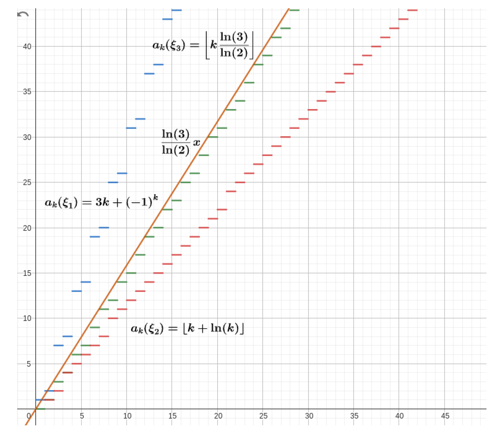
Figure 2.
Orbits of for .
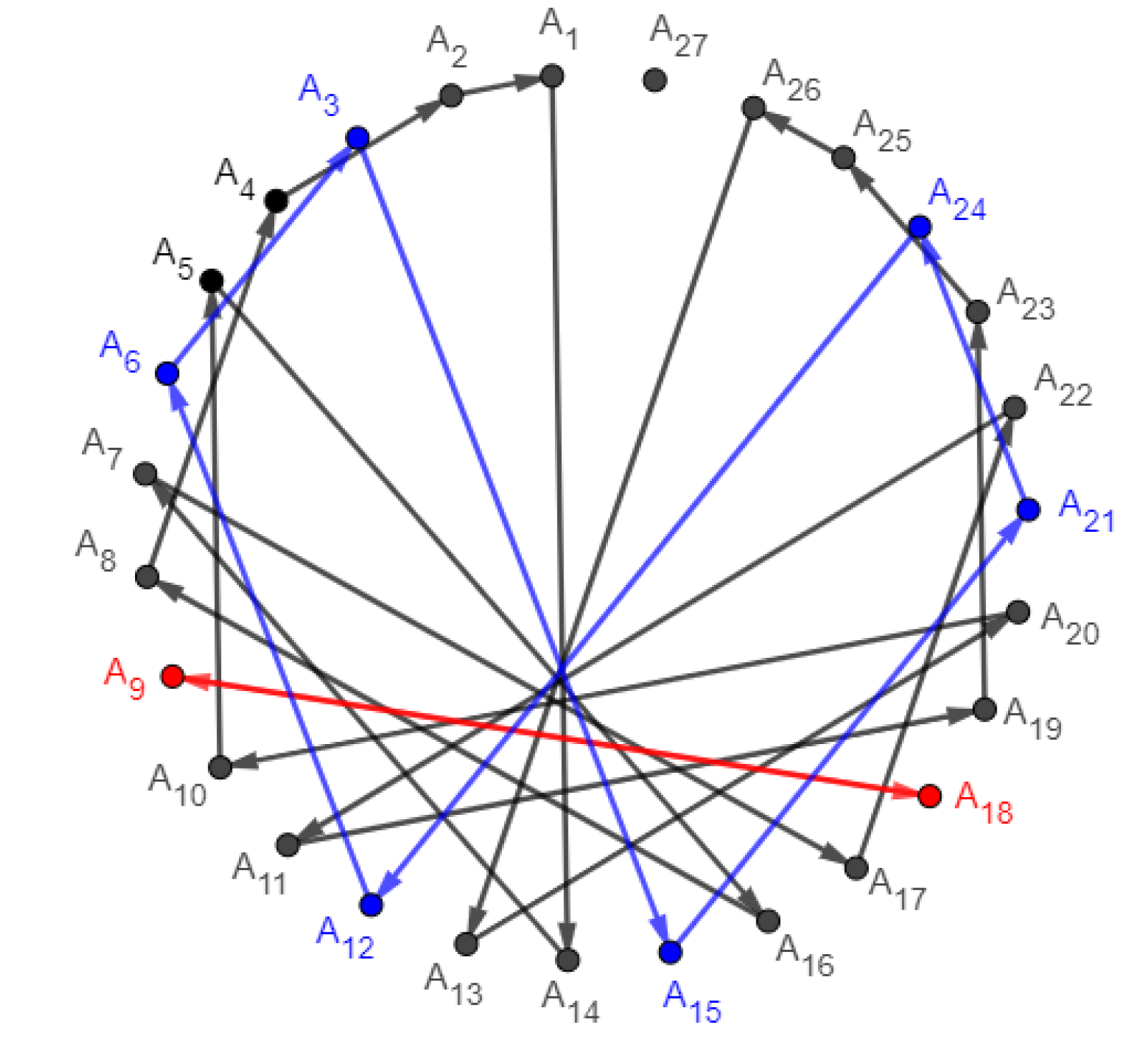
Disclaimer/Publisher’s Note: The statements, opinions and data contained in all publications are solely those of the individual author(s) and contributor(s) and not of MDPI and/or the editor(s). MDPI and/or the editor(s) disclaim responsibility for any injury to people or property resulting from any ideas, methods, instructions or products referred to in the content. |
© 2026 by the authors. Licensee MDPI, Basel, Switzerland. This article is an open access article distributed under the terms and conditions of the Creative Commons Attribution (CC BY) license (http://creativecommons.org/licenses/by/4.0/).
Copyright: This open access article is published under a Creative Commons CC BY 4.0 license, which permit the free download, distribution, and reuse, provided that the author and preprint are cited in any reuse.