
Submitted:
12 August 2024
Posted:
14 August 2024
You are already at the latest version
Abstract
In this study a novel approach of designing automatic control systems with the help of AI tools is proposed. Given plant dynamics, expected references, and expected disturbances, design of optimal neural-network based controller is done automatically. Several common reference types are studied including step, square, sine, sawtooth and trapezoid functions. Expected reference-disturbance pairs are used to train the system for finding optimal neural-network controller parameters. A separate test set is used to test the system for unexpected reference-disturbance pairs to show the generalization performance of the proposed system. Parameters of a real DC motor are used to test the proposed approach. Real DC motor’s parameters are estimated using particle swarm optimization (PSO) algorithm. Initially, a proportional-integral (PI) controller is designed using PSO algorithm for finding simple controller’s parameters optimally and automatically. Starting with neural-network equivalent of optimal PI controller, optimal neural-network controller is designed using PSO algorithm for training again. Simulations are conducted with estimated parameters for diverse set of training and test patterns. Results are compared with optimal PI controller’s performance and reported in the corresponding section. Encouraging results are obtained suggesting further research in the proposed direction.
Keywords:
Automatic control
; artificial intelligence
; controller growing
; neural-network based controller
; disturbance rejection
; robust control
; DC motor
1. Introduction
1.1. Automatic Control Concepts
Automatic control is interested in achieving desired performance for dynamic systems [1]. Dynamic system under control is called plant. Output of plant is measured with some kind of sensor and compared with desired output which is given as reference input. The difference between desired output and real output is called error signal and is the main information used in most of automatic control systems. The block diagram of a typical automatic control system is shown in Figure 1 below.
Aim of the controller is to minimize the error signal which is the difference between reference and output of plant. In order to design the controller mathematical model of the plant is derived first. Plants are generally fall into one of the two main classes: linear and non-linear. Linear plants are easier to control since their mathematical models are linear differential equations which is much easier to analyze mathematically.
Disturbance, also known as external disturbance, is a very important concept for automatic control systems. In order to have a practically useful working system, controller must be robust to external disturbances especially to expected ones. An important parameter of performance is disturbance rejection which represents performance of system under expected disturbances.
Automatic control systems date back to 19th century [2]. During World War I and especially World War II, significant advances were made in automatic control applications. With the advances in computer technology, modern control research gained an acceleration and various types of applications emerged. Applications include motor control [3,4,5,6,7], robot manipulator control [8,9,10,11,12,13,14], wheeled mobile robot control [15,16,17,18], legged mobile robot control [19,20], quadcopter control [21,22] among many others.
1.2. Intelligent Control Systems
Artificial intelligence (AI) has two main schools of thought: classical AI and machine learning. In classical AI, knowledge is hard coded into system by domain experts in terms of domain rules. This approach requires extensive human effort to encode the domain knowledge to computer and is restricted to well structured applications mainly. In a more recent approach, namely machine learning (ML) approach, knowledge is learnt automatically from data by computer.
In ML, there are several types of problems. In supervised learning, training data is labeled by humans and computer learns relation between data and labels. In unsupervised learning, training data is not labeled, so computer tries to find clusters of data with similar properties by some criteria. In reinforcement learning, there is no label for data but only a partial supervision about the consequences of actions as positive or negative so that the computer can learn the best actions leading to most positive results.
One important concept in ML is complexity of system model that computer uses to map data to classes or clusters. Selection optimal complexity of system model is important because if selected model is too simple, it cannot model the underlying process detailed enough. On the other hand, if the selected model is too complex, it can learn noises in training samples instead of parameters in the underlying process. This phenomenon is called overfitting and is a major concern in solutions to ML problems. System with optimal complexity has high generalization performance, which is another important ML concept of performance on the unseen data.
Intelligent control systems utilizing AI especially ML are studied extensively in literature. In [17], speed control of non-holonomic robots is achieved through adaptive gain scheduling and fuzzy multimodel intelligent control and two control strategies are compared. Both implementations are found to have satisfactory performance while that of intelligent controller is found to be higher. In [23], fuzzy intelligent control of servo press systems is studied. Step response experiments and sine tracking experiments are performed and results are reported. In [24], intelligent control research for power systems is reviewed. Studies using artificial neural networks (ANN), fuzzy logic, expert systems and evolutionary methods are reported. In [25], a novel robust innovative optimal robust control method for mobile robots is proposed. Kinematic model of a wheeled mobile robot is derived and a Lyapunov function is used for ensuring control stability. In [26], position tracking control of mobile robots is accomplished using neural network based fractional order sliding mode control. Radial basis function neural network is used to deal with nonlinear dynamics.
1.3. DC Motor Control
Since effective control of DC motor is crucial for performance of many robotic and automation systems, it is widely studied in the literature. In [27], a fuzzy-based predictive PID controller for controlling the speed of DC motor is proposed. Mathematical model of DC motor is derived using corresponding physical laws. Three stages of fuzzy controller, fuzzification, inference and defuzzification, are implemented as components of the controller. Fuzzy based PID controller is combined with receding horizon controller and it is shown that performance of proposed controller is higher than PID controller, fuzzy based PID controller and receding horizon controller implemented separately. In [28], a nonlinear PI controller for speed control of DC motor is proposed. An exponential block placed in front of PI controller introduces nonlinearity to the control system improving controller performance. Salp swarm optimization algorithm [29] is used to tune the parameters of the proposed controller. Experiments are conducted on real DC motor coupled with real DC generator for disturbance generation and results are reported. In [30], sliding mode control is used for performance improvement of DC servo motor. Closed loop control system succeeds to achieve first order system performance and maximum overshoot is reduced.
In this study, an automatic design technique for automatic control of DC motor plant is proposed. DC motor is a popular electrical actuator used in especially robotic systems. Its ease of control due to its simplicity makes it preferable in most industrial applications. Robot arms, mobile robots, CNC machines, 3D printers and many other electromechanical equipment are eligible for DC motor use as actuators. Note that DC motors are generally used with gearboxes to reduce speed and increase torque. As speed and position sensors there are many options available but optical encoder is among the most popular ones. Below is given block diagram of a typical DC motor in Figure 2.
As shown in Figure 2, DC motor consists mainly of three parts: electrical, mechanical and electromagnetic coupling. Electrical part consists of armature resistance and armature inductance. Mechanical part consists of rotor inertia and viscous friction due to bearings. In between there is an electromagnetic coupling due to back-emf force denoted by eb.
Mathematical model of the DC motor is derived using corresponding physical laws as shown in equations below.
where Va is armature voltage, ia is armature current, Ra is armature resistance, La is armature inductance, eb is back-emf voltage, Kω is back-emf constant, Km is motor torque constant, ω is rotor angular speed, Tm is motor torque, J is rotor inertia, b is viscous friction constant and Tl is load torque.
If we organize these four equations into proper order and make necessary replacements, we have a second order system from armature voltage input to rotor angular speed output. Making an additional assumption that La << Ra , that is armature inductance is much less than armature resistance, which is valid for most practical motors, we have a first order system from voltage input to angular speed output, which can be represented by the following transfer function:
which has only two parameters: constant coefficient c1 and constant coefficient c0.
A real DC motor’s parameters are estimated using parameter estimation experiments and following parameters are found using PSO algorithm:
c1=0.00253256, c0=0.09365946
Parameters of optimal PI controller are also found using PSO algorithm and are given as follows:
Kp=1.5, Ki=4980.0
Real DC motor setup used to estimate parameters of real DC motor is shown in Figure 3 below.
Note that real DC motor system consists mainly of three parts. DC motor itself, optical encoder to measure the speed of the motor and gear reduction mechanism to increase the output torque.
Optical encoder subsystems consists of a rotating disc with holes on it, an infrared (IR) transmitter and an IR receiver. Below is shown a close-up photo of the optical encoder used in this study in Figure 4.
IR transmitter sends continuous IR light to the IR receiver. In between the IR transmitter and IR receiver there is a rotating disc with known number of holes on it. The rotating disc is connected to the shaft of the DC motor so rotates at the same speed as the motor. As the disc rotates, IR light falling on the IR receiver is modulated in square wave form period of which depends on the speed of the motor. By calculating the period of the square wave, the speed of the motor is measured.
The gear reduction mechanism is important in many robotic and automation systems in order to obtain required torque to actuate the system. Output of gear reduction system is generally connected to the load which depends on the application. For robot arms, this may be joints connecting each sequential link. for wheeled mobile robots, wheels may be connected to the output shaft of the gear reduction mechanism. For walking mobile robots, again joints of legs may be connected to the shaft. Note that reduction ratio effects the output torque and depends on the application requirements.
In the above-mentioned applications of DC motors, loads vary in time as the system operates. The load to each DC motor is assumed to be external disturbance in this study. Several external disturbance types are applied to the system and results are observed and reported below.
2. Materials and Methods
2.1. Proposed System
Given plant dynamics, expected references, and expected disturbances, an optimal neural-network based controller is designed automatically using the proposed system. The optimal neural-network based controller is composed of two parts and is shown in Figure 5 below.
The first part is the optimal PI controller whose parameters are found using PSO algorithm. The second part is used for fine tuning of the system and has single layer neural-network structure. The input-output relations of the two controllers are as follows:
where e is the error signal which is the difference between reference and output.
Here, tpast and tfuture are past and future window size in terms of sampling time, w’s are neural-network weights, ω’s are plant’s output and ωref’s are references.
Note that this structure is theoretically equivalent to controller with only neural-network part but it is observed that using purely neural-network controller leads to difficult tuning of weights with sometimes unstable results. So, the controller is divided into two parallel parts with optimal PI controller is handling coarse error signals and neural-network part is improving with fine-tuning of the controller output.
2.2. Past and Future Windows
Input to the neural-network based controller is past, current and future references and past and current measurements as shown in Figure 6 below. Two time windows with different scales are used to capture the inputs to the system. The past window is larger than the future window. The past window has both reference and measurement values. The future window has only reference values since measurements of future can not be known in advance. Fixed sampling time of 1 ms is used for all experiments. As an example, with a past window size of 50 ms and a future window size of 20 ms, total number of inputs to the neural-network is 123. Sizes of windows can be changed if required by the application and optimal size of windows is another research topic of future studies.
2.3. Training Neural-Networks with PSO
Optimal weights of neural-network are found using PSO algorithm. Each reference-disturbance pair in training set is input to the system and experiments are conducted. Performance of system is measured using absolute total error metric.
PSO is an iterative optimization algorithm [31]. Vector variable to be optimized is represented by several particles. Particles are initialized randomly from a distribution. Each particle also has a velocity. Position update is simply done by adding velocity of the particle to the previous position. In each iteration, velocity of each particle is updated according to a well-defined rule. Velocity update rule includes three components. First component is calculated using previous velocity of the particle and represents momentum in a sense. Second component is calculated using particle’s known best point up to that iteration. Third component is calculated using global known best point of all particles. In this way randomly initialized particles search through parameter space for an optimum point in a systematic way. Below are the formulas for PSO updates in each iteration.
where x is particle’s position, v is particle’s velocity, p is particle’s known best point up to this iteration, g is global best point of all particles up to this iteration and c’s are constants multiplied by random numbers.
2.4. Discretization and Implementation of System
Discretization and simulation of the system is implemented using the trapezoid rule for differentiation [32]. So, derivative of the state variable is calculated from mathematical model of the system and the state variable, which is the speed of the motor, is calculated using the following formula iteratively:
Here, Δt is taken to be 1 millisecond, to be much lower than time constant of the plant, to minimize discretization errors.
3. Results
Five types of functions are used for references and disturbances: step, square, sine, sawtooth and trapezoid. Below are shown each function in Figure 7.
For step signal there is only one parameter and that is amplitude. For square, sin and sawtooth signals there are two parameters which are amplitude and frequency. For trapezoid signal there are three parameters namely maximum, acceleration and deceleration.
For training, ten different reference and ten different disturbance signals are used. This makes up hundred total reference-disturbance pairs totally. Below are given reference and disturbance signal parameters in Table 1 and Table 2, respectively.
A particle swarm size of 100 is used for training neural-network based controller for 1000 epochs. A optimal neural weight vector of size 123 is obtained with the following values:
g= [[-2.00956934e-02, 2.28251818e-02, 3.66802550e-03, 4.68787594e-03,
1.10714396e-02, -1.25274995e-03, -1.10151555e-02, 7.51440490e-02,
-1.35266461e-02, -2.01238715e-02, 5.46645054e-02, -6.47748694e-03,
2.40590535e-02, 1.97057222e-02, 5.17743275e-02, 1.81642138e-02,
4.33055085e-02, 1.74264836e-02, -4.58121589e-03, 1.42641135e-02,
-5.47776784e-04, -1.76951475e-03, 1.28168151e-02, 2.82062853e-02,
-1.77549715e-03, 1.81045855e-02, 5.28164547e-02, 2.44388379e-02,
-2.53992993e-02, 2.23594722e-05, -2.43687957e-02, -7.82207853e-02,
-1.04065066e-02, -1.26254889e-01, 3.25520224e-03, 1.74701081e-02,
-4.47201247e-03, 1.54930364e-03, -2.17759436e-02, 1.09310672e-01,
1.88470285e-01, 1.53151263e-01, 2.12573135e-01, 5.96647710e-02,
-6.36103418e-03, -1.65250932e-03, 4.89734504e-02, -4.26310941e-03,
1.64341826e-03, -5.74545106e-05, -6.14562688e-01, -8.89053434e-03,
-8.76923913e-04, 2.78282565e-02, -7.14593811e-02, 2.30802202e-02,
4.75389489e-02, 3.08541814e-03, -1.33222498e-03, 4.06371354e-03,
-4.34424866e-02, 9.25887701e-02, -1.17017702e-03, -3.28774384e-02,
5.91127735e-03, -6.76456032e-02, 3.54275769e-03, -2.80618073e-02,
-8.29980821e-02, -4.68078831e-02, -7.70450798e-03, -5.71033232e-04,
-1.97019313e-01, 4.10303154e-03, 5.82616963e-05, -9.41320891e-03,
1.49802579e-01, 3.78894107e-03, -5.41212802e-01, -2.03641023e-01,
6.36523382e-04, -4.50341962e-02, -3.60406881e-01, -3.54286361e-02,
-1.45335544e-02, -8.99566061e-02, 1.89285696e-01, 2.08332606e-01,
-5.91208362e-03, 2.05832348e-02, -2.71000803e-02, 1.92909940e-02,
9.39732840e-01, -4.22809155e-02, -1.97117429e-02, -2.09135482e-02,
-1.09053803e-02, 1.60087125e-03, -1.12127972e-02, 1.26364099e-01,
-1.46189620e-03, 4.01717382e-02, -3.45090396e-01, 1.69375043e-02,
1.18870052e-03, 1.29719444e-02, 4.57404515e-02, 6.09297038e-02,
-1.67111878e-02, 2.74538418e-02, 7.76283972e-02, -9.87016593e-03,
9.83296904e-03, 9.26160487e-03, -1.33904678e-01, -4.46698801e-02,
-6.22031478e-02, -2.08484381e-02, -1.36635522e-03, 2.37264064e-02,
8.05530251e-02, 6.80355357e-02, -1.95685395e-02]]
Average error for optimal PI controller for training set is obtained to be 1.5201955398258502 rad/s. Average error for optimal neural-network based controller for training set is reduced to 1.3890762003883137 rad/s. Hence an approximately 8,6 percent reduction in average error is observed for training set.
Note that training set corresponds to the expected reference-disturbance pairs. If the expected reference-disturbance pairs are estimated correctly, resulting controller will be more robust.
Below are some examples of system outputs of PI and neural-network based controllers for several reference-disturbance pairs.
In Figure 8 below, the result of the experiment run using the following reference-disturbance pair is shown.
Training reference type= step
Training reference amplitude= 100.0
Training reference frequency= 0.0
Training reference acceleration= 0.0
Training reference deceleration= 0.0
Training disturbance type= sine
Training disturbance amplitude= 3.0
Training disturbance frequency= 20.0
Training disturbance acceleration= 0.0
Training disturbance deceleration= 0.0
In this example configuration, neural-network based controller has clearly higher performance than optimal PI controller with the following costs:
Cost PID= 11.036012620309064
Cost ANN= 4.474398851829462
In another scenario with the following reference-disturbance pairs, neural-network based controller has higher performance than optimal PI controller. Result is shown in Figure 9 below.
Training reference type= sine
Training reference amplitude= 100.0
Training reference frequency= 3.0
Training reference acceleration= 0.0
Training reference deceleration= 0.0
Training disturbance type= step
Training disturbance amplitude= 3.0
Training disturbance frequency= 0.0
Training disturbance acceleration= 0.0
Training disturbance deceleration= 0.0
Cost PID= 4.365012134434239
Cost ANN= 3.639447860741749
These results show that for expected reference-disturbance pairs neural-network based controller has clearly higher performance than optimal PI controller.
An important concept in artificial intelligence is generalization performance which means the performance of the system for examples unseen during training. So, in order to test the generalization performance new examples different from training set must be shown to the system. This new set is called test-set and has samples different from that of training set. Below is shown the reference-disturbance signal values for test set used in this study.

Table 3.
Reference signal values for test set.
| Signal Number | Type | Amplitude (rad/s) | Frequency (Hz) | Acc. Time (ms) | Dec. Time (ms) |
|---|---|---|---|---|---|
| 1 | step | 100 | NA | NA | NA |
| 2 | square | 100 | 2 | NA | NA |
| 3 | square | 100 | 3 | NA | NA |
| 4 | square | 100 | 4 | NA | NA |
| 5 | square | 100 | 5 | NA | NA |
| 6 | square | 100 | 6 | NA | NA |
| 7 | square | 100 | 8 | NA | NA |
| 8 | square | 100 | 10 | NA | NA |
| 9 | trapezoid | 100 | NA | 200 | 200 |
| 10 | trapezoid | 100 | NA | 100 | 100 |
Table 4.
Disturbance signal values for test set.
| Signal Number | Type | Amplitude (Volts) | Frequency (Hz) | Acc. Time (ms) | Dec. Time (ms) |
|---|---|---|---|---|---|
| 1 | square | 1 | 5 | NA | NA |
| 2 | square | 1 | 10 | NA | NA |
| 3 | square | 1 | 20 | NA | NA |
| 4 | square | 2 | 5 | NA | NA |
| 5 | square | 2 | 10 | NA | NA |
| 6 | square | 2 | 20 | NA | NA |
| 7 | sawtooth | 1 | 5 | NA | NA |
| 8 | sawtooth | 1 | 20 | NA | NA |
| 9 | sawtooth | 2 | 5 | NA | NA |
| 10 | sawtooth | 2 | 20 | NA | NA |
Average error for optimal PI controller for test set is obtained to be 53.30442198786117 rad/s. Average error for optimal neural-network based controller for test set is reduced to 52.893195124124276 rad/s. A slight reduction in error is observed for unexpected reference-disturbance pairs. Note that this small improvement in error for unexpected reference-disturbance pairs is not that crucial but gives an extra advantage to proposed system since the main objective is to design automatic controller automatically for expected reference-disturbance pairs. But this also shows that the proposed system has better generalization performance than optimal PI controller.
4. Discussion
4.1. Performance Issues
Results clearly show that proposed method has very promising performance especially for expected reference-disturbance pairs. As an automatic design method for automatic controller design, the proposed method automates the engineering process by largely performing critical tasks. Expected reference-disturbance pair selection is important in the performance of the proposed automatic control system. Even in the unexpected reference-disturbance pairs, the proposed system shows superior performance than optimal PI controller ensuring acceptable generalization performance in AI terms.
Note that proposed system shows superior performance especially under difficult disturbances which is important for realistic missions of robust systems. Under low disturbance conditions almost any rational controller will have acceptable performance but real quality of the controller is seen under harsh conditions. For example, for an air vehicle carrying humans, either fixed wing or mobile wing, it is important to fly safely under relatively high-power external wind disturbance in order to be utilized more effectively.
4.2. Implementation Issues
Expected reference-disturbance pairs can be generated in several different ways. For example, for an aircraft autopilot application, commands of a human pilot can be saved for several real flights as expected references and for realistic disturbances, a neural-network based disturbance observer can be used to estimate the real disturbances during real flights. Similarly, for drone applications, references of a human pilot can be saved for realistic references and again a neural-network based disturbance observer can be used to estimate the real disturbances to occur in real flights under various air conditions. Information from real experts can also be incorporated into realistic reference-disturbance pair generation. Realistic simulations with complex realistic mathematical models can also be used for realistic reference-disturbance pair estimation.
4.3. Ethical Issues
Usage of AI to replace humans is discussed extensively in terms of ethics and many people have concerns for losing their jobs to machines. In fact, AI based robot doctors giving more reliable diagnosis results should not be taken as a threat to human doctors’ professions. AI designed automatic controllers controlling human carrying air vehicles more reliably must be welcome to humanity’s profession world just as well. As a matter of fact, it should be not scientists’ concerns to advance humanity’s knowledge on any branch of science including AI because as in any branch of science, advances in AI have very high benefits to humanity and adds to humanity’s overall wealth. It is up to leaders and politicians how to share the overall wealth gained by using AI and other scientific advances and global decisions involving every single nation must be taken to ensure fair and humanely distribution of wealth and income of humanity. Just like crashing all dams may have positive side effect of creating lots of human jobs but is not a rational decision, stopping or slowing production of AI tools is not a rational solution for unfair wealth distribution problem.
Funding
This research received no external funding.
Data Availability Statement
We encourage all authors of articles published in MDPI journals to share their research data. In this section, please provide details regarding where data supporting reported results can be found, including links to publicly archived datasets analyzed or generated during the study. Where no new data were created, or where data is unavailable due to privacy or ethical restrictions, a statement is still required. Suggested Data Availability Statements are available in section “MDPI Research Data Policies” at https://www.mdpi.com/ethics.
Conflicts of Interest
The author declares no conflicts of interest.
Appendix A
All simulations of the study are implemented in Python programming language in Anaconda environment. Jupyter Notebook is used as IDE. Below are given important parts of the code.
#Function implementing DC motor dynamic behavior
def DCMotorPlant(w_n_1, Va, disturbance):
#Forward system model starts here.
# Compare the Armature Voltage with Max/Min Value
if Va > VaMax:
Va = VaMax
if Va < VaMin:
Va = VaMin
#Simulation of DC Motor
dw_dt = -(coefficient0/coefficient1)*w_n_1+(1/coefficient1)*(Va+disturbance)
w = w_n_1 + deltaT*dw_dt
return w
#Function implementing PI controller
def pidController(wref_n, w_n_1, intError, prevError, PIDcontrollerParameters):
KP=PIDcontrollerParameters[0]
KI=PIDcontrollerParameters[1]
KD=PIDcontrollerParameters[2]
error = wref_n - w_n_1
intError = intError + error*deltaT
if intError>intErrormax:
intError=intErrormax
if intError<intErrormin:
intError=intErrormin
derError = (error - prevError)/deltaT
prevError = error
if derError>derErrormax:
derError=derErrormax
if derError<derErrormin:
derError=derErrormin
pidOut = KP*error + KI*intError + KD*derError
return pidOut, intError, prevError
#Function implementing single experiment performance
#with given reference-disturbance pair
def performExperiment(controllerType, PIDcontrollerParameters, ANNcontrollerParameters, reference, disturbance):
tempReference = np.zeros((int(tmax/deltaT)+1000))
tempReference[0:int(tmax/deltaT)] = reference[:]
inputToANNController = np.zeros((numberOfStateVariables*pastAndCurrentWindowSizeInTermsOfSamples+numberOfReferenceVariables*totalWindowSizeInTermsOfSamples+1,1))
intError=0
prevError=0
controllerOutput=0
n=0
w = np.zeros((int(tmax/deltaT)))
for n1 in np.linspace(0, n1max, num=n1max-1):
n=n+1
controllerOutput, intError, prevError = pidController(tempReference[n-1], w[n-1], intError, prevError, PIDcontrollerParameters)
if n<=nPast+1 or controllerType=='PID':
#pidOut will be that of PID controller's output
additiveTerm = 0
else:
#BUILD INPUT TO THE ANN CONTROLLER
inputToANNController[0,0] = 1 #1
inputToANNController[1:nPast+2,0] = w[n-nPast-2:n-1]
inputToANNController[nPast+2:2*nPast+3,0] = tempReference[n-nPast-2:n-1]
inputToANNController[2*nPast+3:2*nPast+3+nFuture,0] = tempReference[n-1:n+nFuture-1]
#HERE THE ANN CONTROLLER
additiveTerm = np.dot(ANNcontrollerParameters.transpose(), inputToANNController)
controllerOutput = controllerOutput + additiveTerm
w[n] = DCMotorPlant(w[n-1], controllerOutput, disturbance[n])
return w
References
- Ogata, K. (2020). Modern control engineering.
- Bissell, C. (2009). A history of automatic control. Springer handbook of automation, 53-69.
- Baidya, D.; Dhopte, S.; Bhattacharjee, M. Sensing system assisted novel PID controller for efficient speed control of DC motors in electric vehicles. IEEE Sensors Letters 2023, 7, 1–4. [Google Scholar] [CrossRef]
- Munagala, V.K.; Jatoth, R.K. A novel approach for controlling DC motor speed using NARXnet based FOPID controller. Evolving Systems 2023, 14, 101–116. [Google Scholar] [CrossRef]
- Saputra, D.; Ma'arif, A.; Maghfiroh, H.; Chotikunnan, P.; Rahmadhia, S. N. Design and application of PLC-based speed control for DC motor using PID with identification system and MATLAB tuner. International Journal of Robotics and Control Systems 2023, 3, 233–244. [Google Scholar] [CrossRef]
- Ekinci, S. , Izci, D., & Yilmaz, M. (2023). Efficient speed control for DC motors using novel Gazelle simplex optimizer. IEEE Access.
- Yıldırım, Ş. , Bingol, M. S., & Savas, S. (2024). Tuning PID controller parameters of the DC motor with PSO algorithm. International Review of Applied Sciences and Engineering.
- Son, J.; Kang, H.; Kang, S.H. A review on robust control of robot manipulators for future manufacturing. International Journal of Precision Engineering and Manufacturing 2023, 24, 1083–1102. [Google Scholar] [CrossRef]
- Han, D.; Mulyana, B.; Stankovic, V.; Cheng, S. A survey on deep reinforcement learning algorithms for robotic manipulation. Sensors 2023, 23, 3762. [Google Scholar] [CrossRef] [PubMed]
- Pistone, A.; Ludovico, D.; Dal Verme, L.D.M.C.; Leggieri, S.; Canali, C.; Caldwell, D.G. Modelling and control of manipulators for inspection and maintenance in challenging environments: A literature review. Annual Reviews in Control 2024, 57, 100949. [Google Scholar] [CrossRef]
- Bilal, H.; Yin, B.; Aslam, M.S.; Anjum, Z.; Rohra, A.; Wang, Y. A practical study of active disturbance rejection control for rotary flexible joint robot manipulator. Soft Computing 2023, 27, 4987–5001. [Google Scholar] [CrossRef]
- Chotikunnan, P.; Chotikunnan, R. Dual design PID controller for robotic manipulator application. Journal of Robotics and Control (JRC) 2023, 4, 23–34. [Google Scholar] [CrossRef]
- Villa-Tiburcio, J.F.; Estrada-Torres, J.A.; Hernández-Alvarado, R.; Montes-Martínez, J.R.; Bringas-Posadas, D.; Franco-Urquiza, E.A. ANN Enhanced Hybrid Force/Position Controller of Robot Manipulators for Fiber Placement. Robotics. 2024, 13, 105. [Google Scholar] [CrossRef]
- Chang, Y.-H.; Yang, C.-Y.; Lin, H.-W. Robust Adaptive-Sliding-Mode Control for Teleoperation Systems with Time-Varying Delays and Uncertainties. Robotics. 2024, 13, 89. [Google Scholar] [CrossRef]
- Kouvakas, N.D.; Koumboulis, F.N.; Sigalas, J. A Two Stage Nonlinear I/O Decoupling and Partially Wireless Controller for Differential Drive Mobile Robots. Robotics. 2024, 13, 26. [Google Scholar] [CrossRef]
- Bernardo, R.; Sousa, J.M.C.; Botto, M.A.; Gonçalves, P.J.S. A Novel Control Architecture Based on Behavior Trees for an Omni-Directional Mobile Robot. Robotics. 2023, 12, 170. [Google Scholar] [CrossRef]
- Miquelanti, M.G.; Pugliese, L.F.; Silva, W.W.A.G.; Braga, R.A.S.; Monte-Mor, J.A. Comparison between an Adaptive Gain Scheduling Control Strategy and a Fuzzy Multimodel Intelligent Control Applied to the Speed Control of Non-Holonomic Robots. Applied Sciences 2024, 14, 6675. [Google Scholar] [CrossRef]
- Rodriguez-Castellanos, D.; Blas-Valdez, M.; Solis-Perales, G.; Perez-Cisneros, M.A. Neural Robust Control for a Mobile Agent Leader–Follower System. Applied Sciences. 2024, 14, 5374. [Google Scholar] [CrossRef]
- Polakovič, D.; Juhás, M.; Juhásová, B.; Červeňanská, Z. Bio-Inspired Model-Based Design and Control of Bipedal Robot. Applied Sciences. 2022, 12, 10058. [Google Scholar] [CrossRef]
- Chi, K-H. ; Hsiao, Y-F.; Chen, C-C. Robust Feedback Linearization Control Design for Five-Link Human Biped Robot with Multi-Performances. Applied Sciences. 2023, 13, 76. [Google Scholar] [CrossRef]
- Godinez-Garrido, G.; Santos-Sánchez, O.-J.; Romero-Trejo, H.; García-Pérez, O. Discrete Integral Optimal Controller for Quadrotor Attitude Stabilization: Experimental Results. Applied Sciences. 2023, 13, 9293. [Google Scholar] [CrossRef]
- Sonugür, G.; Gökçe, C.O.; Koca, Y.B.; Inci, Ş.S.; Keleş, Z. Particle swarm optimization based optimal PID controller for quadcopters. Comptes rendus de l’Acade'mie bulgare des Sciences 2021, 74, 1806–1814. [Google Scholar]
- He, Y.; Luo, X.; Wang, X. Research and Simulation Analysis of Fuzzy Intelligent Control System Algorithm for a Servo Precision Press. Applied Sciences 2024, 14, 6592. [Google Scholar] [CrossRef]
- Alhamrouni, I.; Abdul Kahar, NH.; Salem, M.; Swadi, M.; Zahroui, Y.; Kadhim, D.J.; Mohamed, F.A.; Alhuyi Nazari, M. A Comprehensive Review on the Role of Artificial Intelligence in Power System Stability, Control, and Protection: Insights and Future Directions. Applied Sciences. 2024, 14, 6214. [Google Scholar] [CrossRef]
- Hu, Y.; Zhou, W.; Liu, Y.; Zeng, M.; Ding, W.; Li, S.; Knoll, A. (2024). Efficient Online Planning and Robust Optimal Control for Nonholonomic Mobile Robot in Unstructured Environments. IEEE Transactions on Emerging Topics in Computational Intelligence.
- Kumar, N.; Chaudhary, K. S. (2024). Neural network based fractional order sliding mode tracking control of nonholonomic mobile robots. Journal of Computational Analysis & Applications, 33(1).
- Freitas, J.B.S.; Marquezan, L.; de Oliveira Evald, P.J.D.; Peñaloza, E.A.G.; Cely, M.M.H. A fuzzy-based predictive PID for DC motor speed control. International Journal of Dynamics and Control 2024, 1–11. [Google Scholar] [CrossRef]
- Çelik, E., Bal, G., Öztürk, N., Bekiroglu, E., Houssein, E. H., Ocak, C., & Sharma, G. (2024). Improving speed control characteristics of PMDC motor drives using nonlinear PI control. Neural Computing and Applications, 1-12.
- Mirjalili, S.; Gandomi, A.H.; Mirjalili, S.Z.; Saremi, S.; Faris, H.; Mirjalili, S.M. Salp Swarm Algorithm: A bio-inspired optimizer for engineering design problems. Advances in engineering software 2017, 114, 163–191. [Google Scholar] [CrossRef]
- Dawane, M.K.; Malwatkar, G.M.; Deshmukh, S.P. Performance improvement of DC servo motor using sliding mode controller. Journal of Autonomous Intelligence 2024, 7. [Google Scholar] [CrossRef]
- Clerc, M. (2010). Particle swarm optimization (Vol. 93). John Wiley & Sons.
- Thomas, G. B. , Weir, M. D., & Hass, J. (2010). Thomas' Calculus: Multivariable.
Figure 1.
Block Diagram of a Typical Automatic Control System.
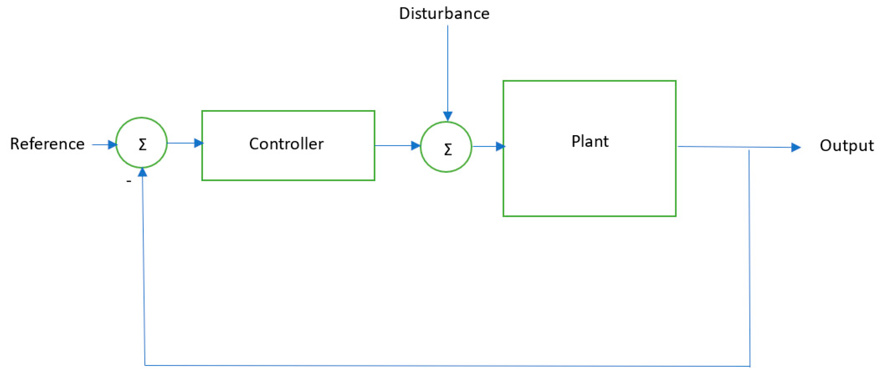
Figure 2.
Block Diagram of a DC Motor System.
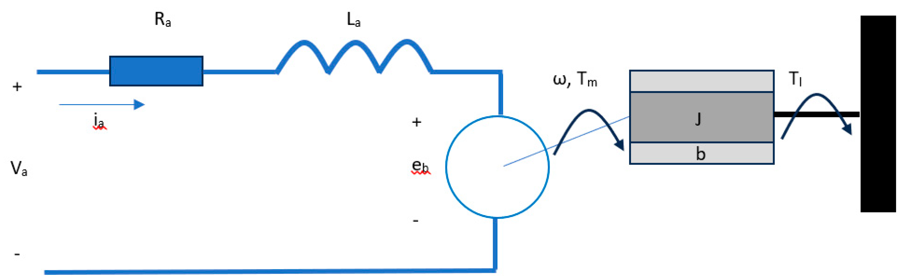
Figure 3.
Real DC Motor Setup Used to Estimate Parameters of Real DC Motor.
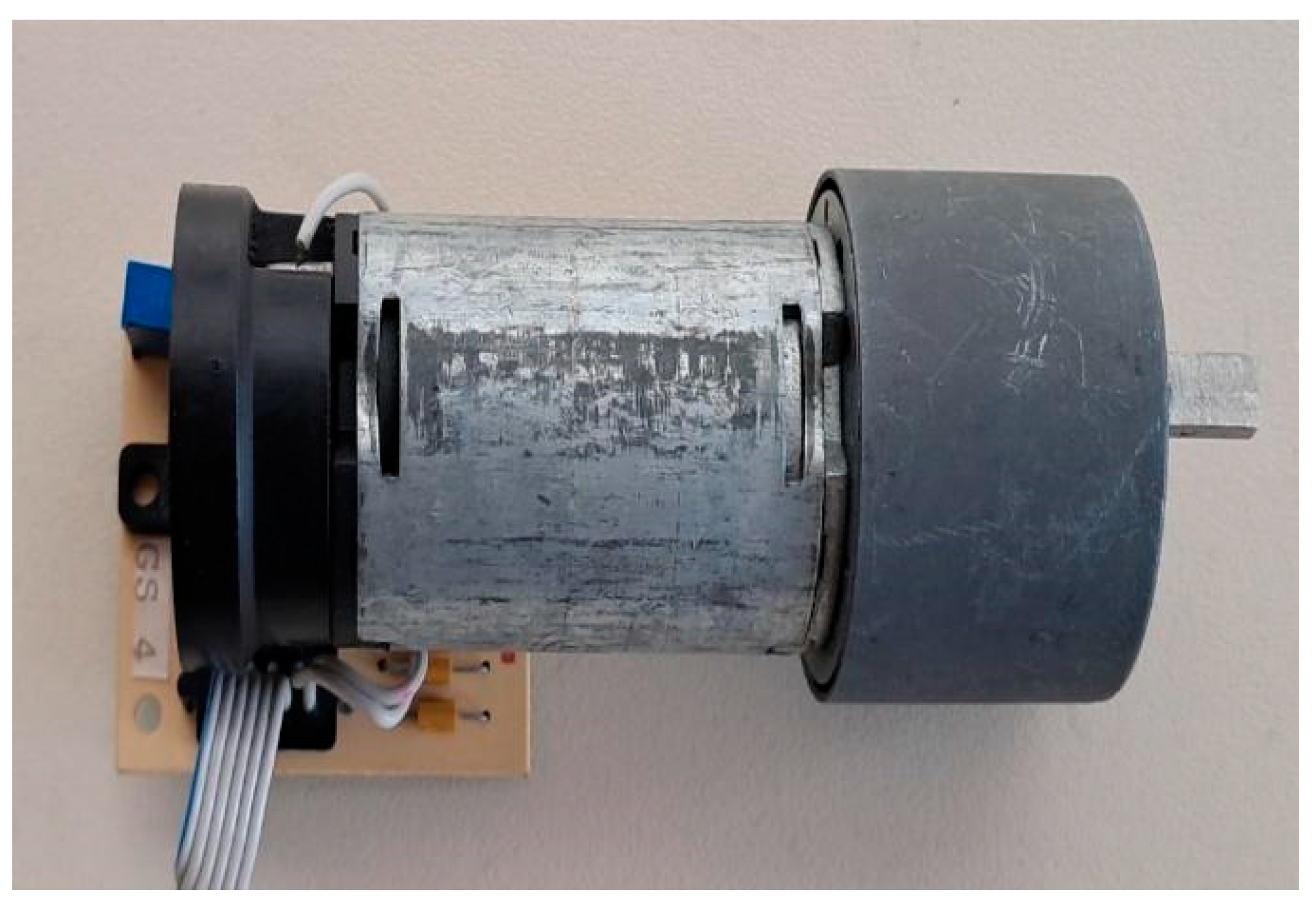
Figure 4.
Close-up photo of optical encoder used to measure speed of the motor.
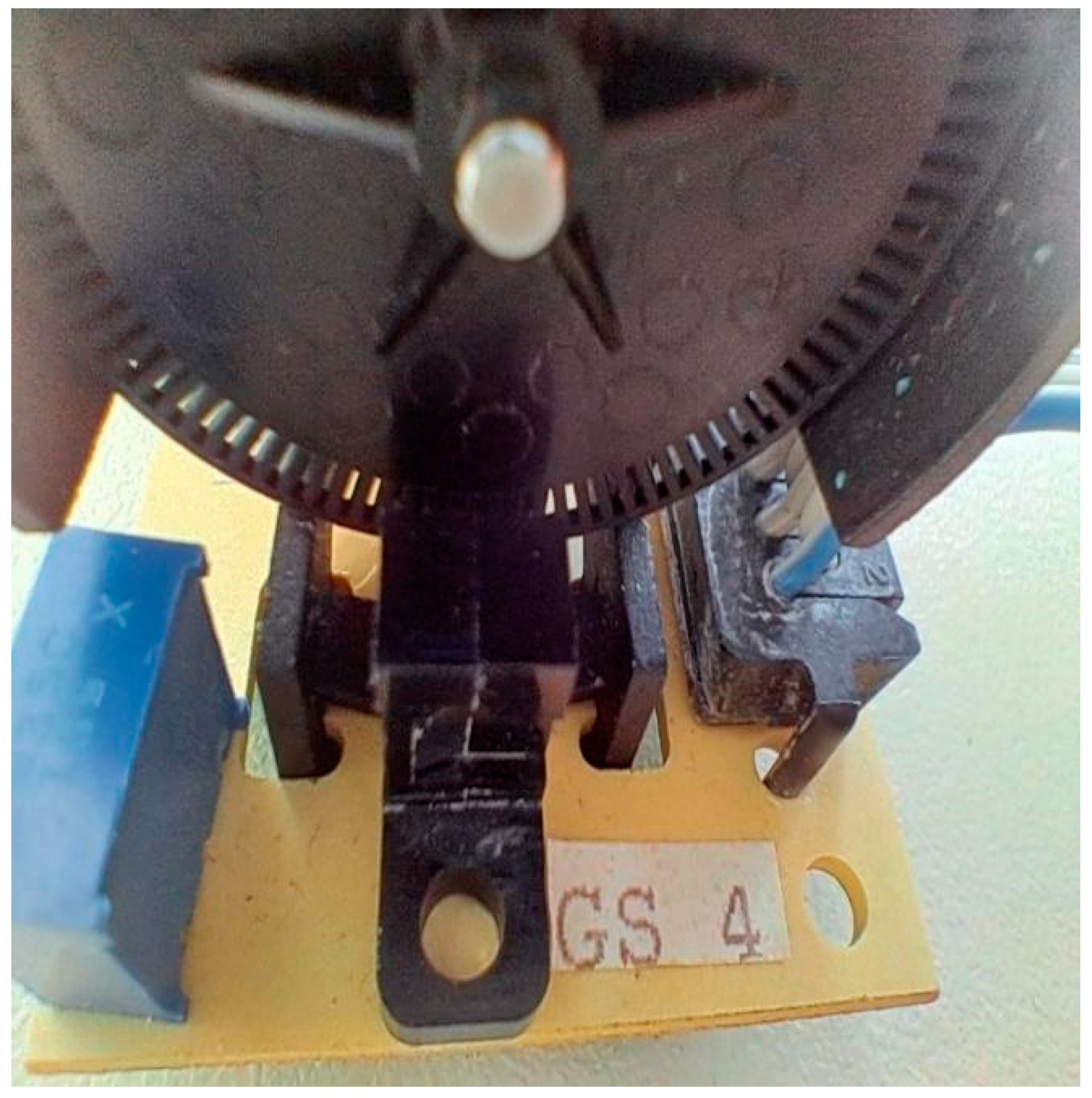
Figure 5.
System with proposed controller structure.
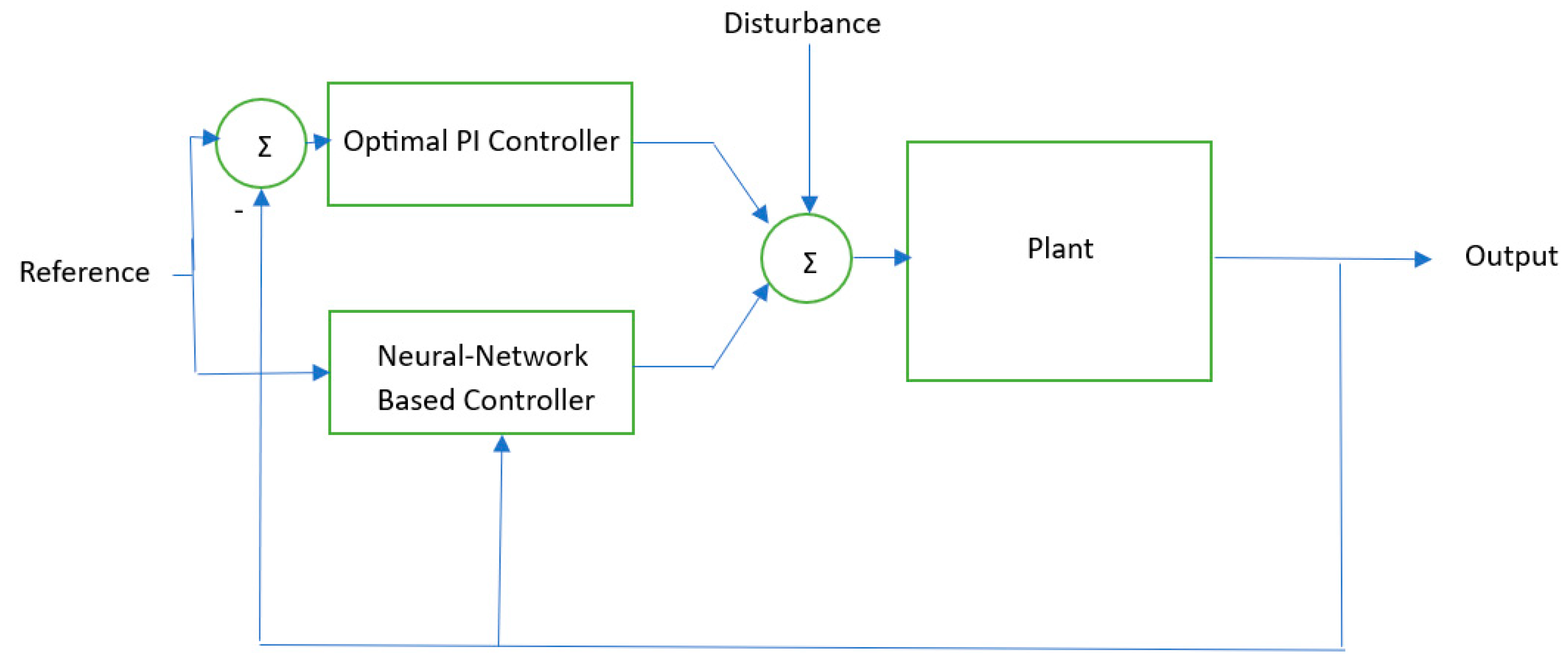
Figure 6.
Input past and future windows illustrated.
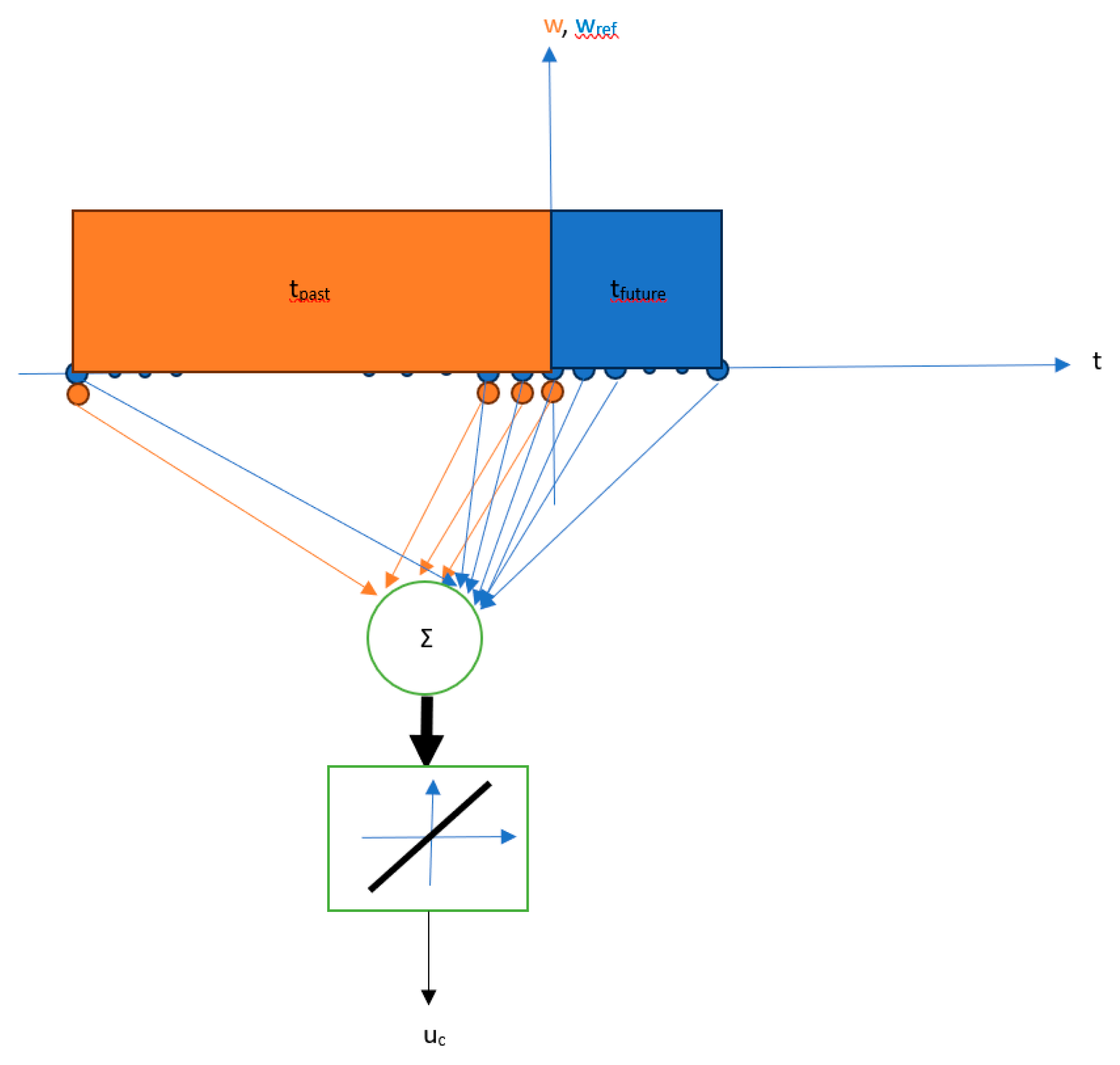
Figure 7.
Five types of functions for references and disturbances.
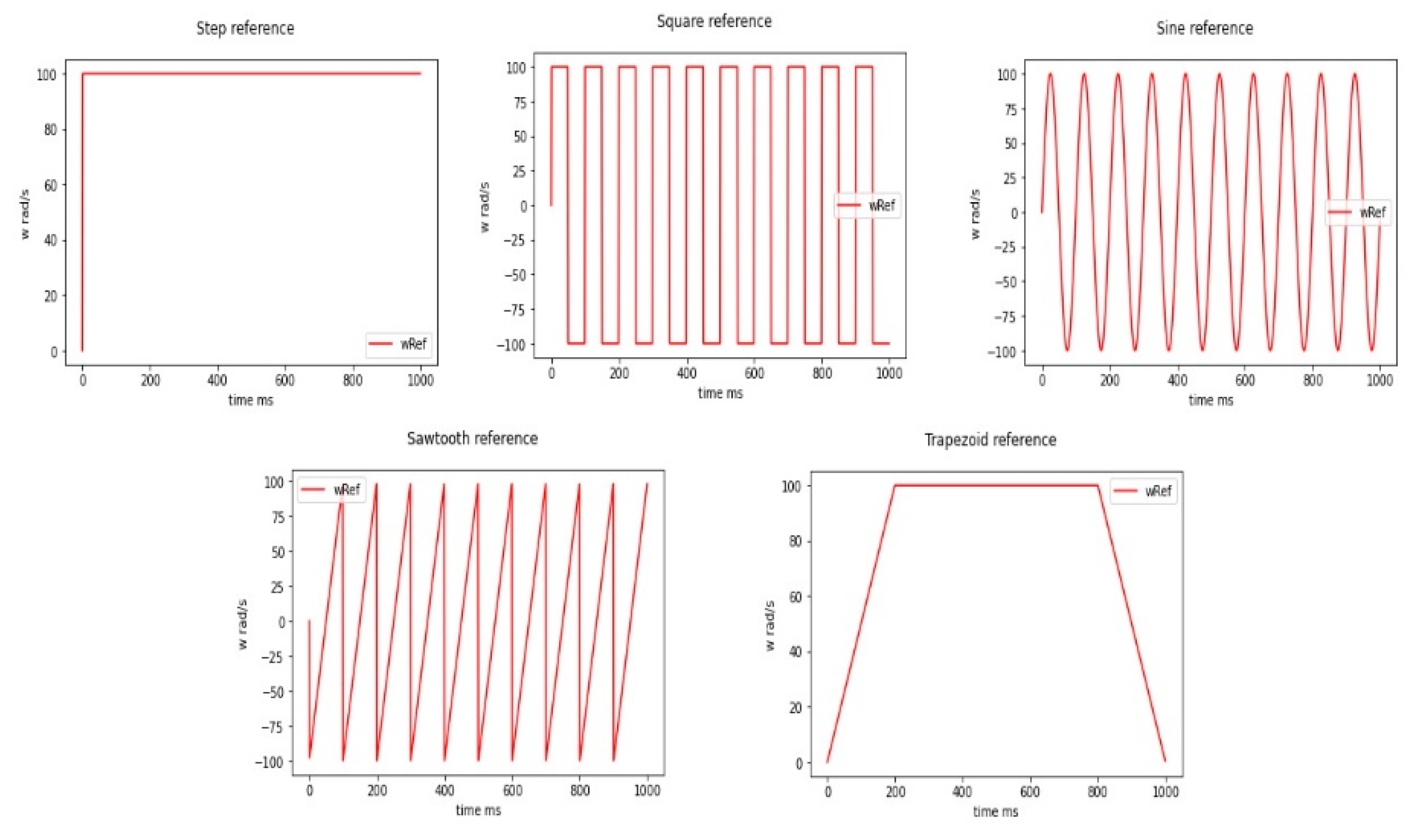
Figure 8.
An illustrative example of neural-controller’s high performance.
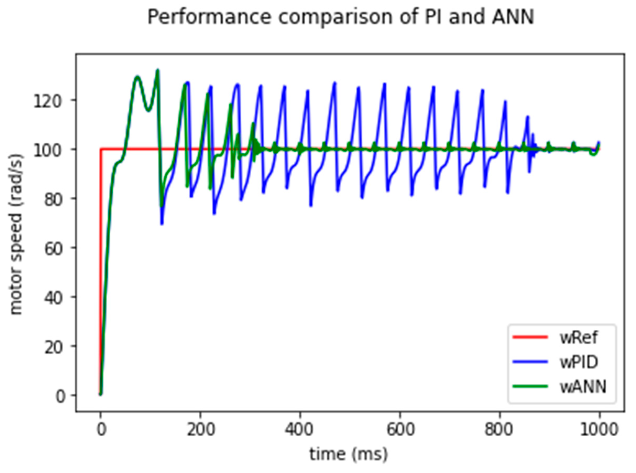
Figure 9.
Another illustrative example of neural-controller’s high performance.
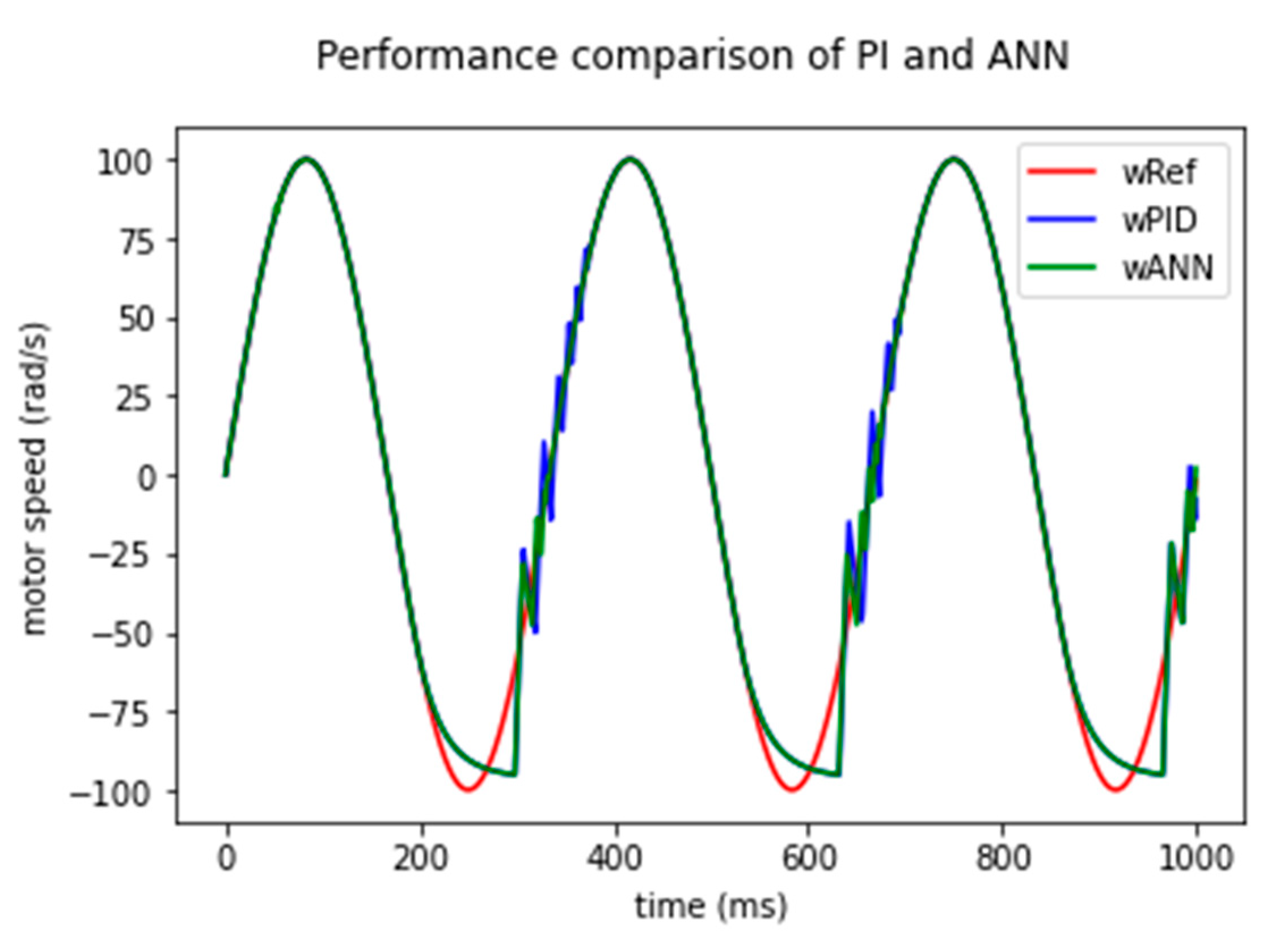
Table 1.
Reference signal values for training set.
| Signal Number | Type | Amplitude (rad/s) | Frequency (Hz) | Acc. Time (ms) | Dec. Time (ms) |
|---|---|---|---|---|---|
| 1 | step | 50 | NA | NA | NA |
| 2 | step | 70 | NA | NA | NA |
| 3 | step | 90 | NA | NA | NA |
| 4 | step | 100 | NA | NA | NA |
| 5 | sine | 50 | 2 | NA | NA |
| 6 | sine | 50 | 3 | NA | NA |
| 7 | sine | 50 | 5 | NA | NA |
| 8 | sine | 100 | 2 | NA | NA |
| 9 | sine | 100 | 3 | NA | NA |
| 10 | sine | 100 | 5 | NA | NA |
Table 2.
Disturbance signal values for training set.
| Signal Number | Type | Amplitude (Volts) | Frequency (Hz) | Acc. Time (ms) | Dec. Time (ms) |
|---|---|---|---|---|---|
| 1 | step | 1 | NA | NA | NA |
| 2 | step | 1,5 | NA | NA | NA |
| 3 | step | 2 | NA | NA | NA |
| 4 | step | 3 | NA | NA | NA |
| 5 | sine | 1 | 5 | NA | NA |
| 6 | sine | 1 | 20 | NA | NA |
| 7 | sine | 2 | 5 | NA | NA |
| 8 | sine | 2 | 20 | NA | NA |
| 9 | sine | 3 | 5 | NA | NA |
| 10 | sine | 3 | 20 | NA | NA |
Disclaimer/Publisher’s Note: The statements, opinions and data contained in all publications are solely those of the individual author(s) and contributor(s) and not of MDPI and/or the editor(s). MDPI and/or the editor(s) disclaim responsibility for any injury to people or property resulting from any ideas, methods, instructions or products referred to in the content. |
© 2024 by the authors. Licensee MDPI, Basel, Switzerland. This article is an open access article distributed under the terms and conditions of the Creative Commons Attribution (CC BY) license (http://creativecommons.org/licenses/by/4.0/).
Copyright: This open access article is published under a Creative Commons CC BY 4.0 license, which permit the free download, distribution, and reuse, provided that the author and preprint are cited in any reuse.


