Submitted:
02 August 2024
Posted:
06 August 2024
You are already at the latest version
Abstract
Research in complex network analysis, including tasks such as information dissemination and link prediction, has traditionally advanced by examining groups of nodes with similar characteristics. In multilayer complex networks, these analyses are performed layer-wise, with each layer representing a distinct feature. However, this approach often neglects interlayer interactions, leading to limited predictive power, underestimation of network resilience, and incomplete identification of influential nodes. This article introduces a novel block modeling technique that integrates dominant features from multiple layers, addressing these shortcomings. Our approach introduces a new centrality metric that combines layer weight and PageRank centrality to identify influential nodes within multilayer networks. Nodes are aggregated into blocks centered around these influencers, accounting for both intra- and interlayer connections. Empirical evaluation of various datasets demonstrates that our method effectively identifies influential nodes, thereby enhancing information dissemination and link prediction across diverse multilayer network structures. This technique offers significant potential for improving decision-making processes in various fields, including social network analysis, transportation systems, and biological networks.
Keywords:
block formation
; multilayer networks
; network analysis
; link prediction
; information dissemination
1. Introduction
Complex networks serve as a model for various real-world systems, including social networks, biological entities, ecological systems, and communication networks. These networks can take many forms, such as citation networks, friendship networks, airline networks, mobile communication networks, and protein-protein interaction networks. One key aspect of these systems is their size, and ranges from thousands to millions of entities. Additionally, entities within these networks interact and evolve in ways that are hard to anticipate, exhibit multiple behaviors, and share multiple relationships.
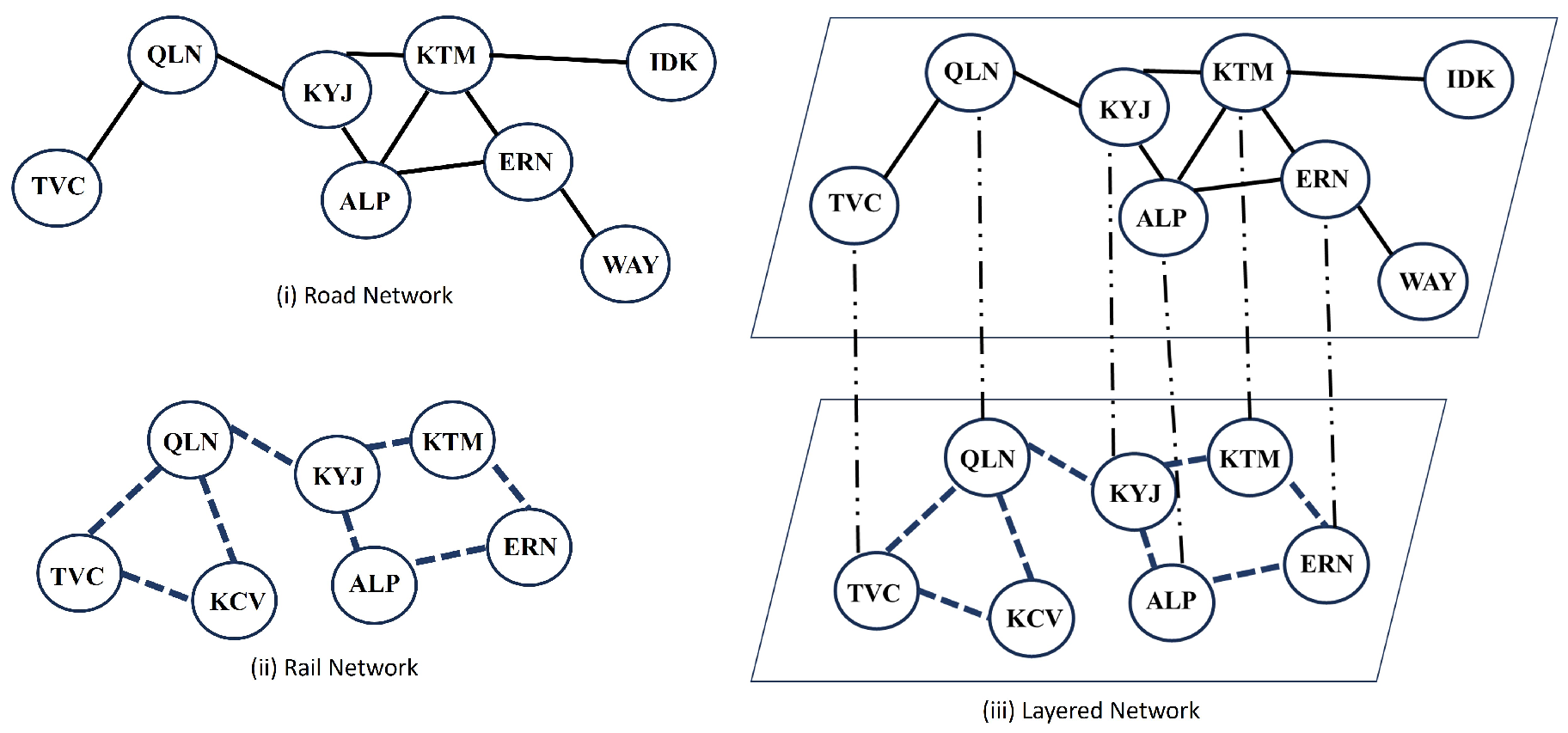
Multilayer networks capture the intricate interplay of interactions and relationships that exist in real-world systems by representing them as a collection of interconnected layers, each corresponding to a distinct type of interaction or relationship. The traditional single-layer network representation may not be sufficient to fully capture the complex interactions and inter-dependencies that exist within Growing Network Models. For instance, in a transportation network, nodes represented as cities can be connected via road and rail networks, resulting in two different interactions between nodes as shown in Figure 1.i and Figure 1.ii. Some of the cities are common to both networks, while others are not. For analyzing both interactions together, such independent representation is insufficient. The emergence of multilayer models was a response to capture such interactions. Each layer represents the interaction within a single network (road or rail), while the link between common nodes of two layers represents that such nodes are part of both networks. Thus, multiple dimensions of the nodes are captured by the multiple layers, each representing distinct types of relationships or attributes. Each layer contributes to the overall structure of the network, and interlayer connections enable the examination of interactions and dependencies between layers, as depicted in Figure 1.iii.
Towards this end, the multilayer network defined by [1] is as given below:
A Multilayer network , is a collection of elementary layers stacked together where each layer denotes an aspect such that are the layers, V represents all the vertices of the network. is a set of nodes specific to a particular layer. It represents the nodes present in a given layer of the multilayer network such that , and , and represents the edges between a pair of vertices, , the edge , denotes the intra layer edge when and denotes the inter-layer edge when .
Several problems in various application domains are of interest to the multilayer network research community. Prominent among them are Information Diffusion, Community detection [2], Link Prediction. Link prediction is used to predict missing or future connections between nodes in a network. It has applications like identifying friendships or connections between users in Social networks and product recommendations [3,4]. In such cases, the existing state-of-the-art is insufficient as they do not consider (i) similarity/dissimilarity between the layers, (ii) the interplay between the layers, and (iii) the evolving interlayer dependencies between the layers. These factors are relevant for capturing heterogeneity, understanding interactions that reflect the intricate web of interactions, and evolving dynamics in complex networks. The state-of-the-art has limitations in addressing the interplay between the layers. Hence we formulate an approach for the heterogeneous multilayer network, having an ability to capture the inherent modular organization present in many real-world networks. The research goals addressed in this article are as follows:
- -
- Identify the prominent nodes influencers in a directed multilayered heterogeneous network.
- -
- The formulation of novel block modeling technique that considers the interplay between the layers and the evolving inter-dependencies around the prominent nodes in the multilayer network.
- -
- Efficacy of block modeling in the analysis of the complex network especially for Information diffusion and Link Prediction.
The advantage of block formation is that each block is formed based on a different set of characteristics shared between the nodes. This helps in integrating the information from various layers, thereby enabling the information diffusion or link prediction application to a better accuracy. The Section 3.1 discusses the identification of influencers across the network. The block formation process around the influencers is elucidated in Section 3.2. We propose the link prediction between the blocks and the information diffusion with the blocks in Section 3.3 and Section 3.4 respectively. The experimental setup and analysis are discussed in Section 5. The observations, findings, and conclusions are discussed in Section 6.
Figure 1.
(i) Network representing the road network (ii) Network Rail Network (iii) Layered Network representing the transportation network (road and rail)
Figure 1.
(i) Network representing the road network (ii) Network Rail Network (iii) Layered Network representing the transportation network (road and rail)
2. Background Study
Complex networks have permeated every aspect of our daily lives, manifesting in various forms such as the World Wide Web [5], the Internet [6], and social friendship networks [7]. A real-world network, modeled as a multilayer network, consists of different layers that represent the diverse types of interactions or relationships. For example, one layer could represent social connections, while another represents professional collaborations. Each layer contributes to the overall structure of the network. Nodes in a multilayer network may have connections across layers. This interlayer connectivity introduces the need to consider not only the within-layer interactions but also the influence of nodes that bridge different layers. Nodes in a multilayer network may have different roles in different layers [8]. Some nodes may be hubs in one layer but less influential in another. Identifying and quantifying these roles are crucial for understanding the multifaceted nature of node centrality.
Centrality is the fundamental metric in network science and finds application in various fields. Centrality aims to identify the most influential nodes in the network by considering various factors. Centrality metrics provide a way to quantify the relative significance of nodes by analyzing their connectivity patterns. Influencers have a significant reach and disseminate information rapidly within a network, and hence are of interest in the context of network analysis.
Different centrality measures, such as degree centrality [9,10], random-walk occupation centrality, betweenness centrality [11], and closeness centrality[12,13], eigenvector centrality [14,15], Katz centrality, and PageRank [16,17], have been developed for monoplex networks [18,19,20,21]. These measures take into account the network’s structure or dynamic processes to evaluate the importance of nodes. By utilizing these centrality metrics, highly connected nodes, strategically positioned nodes, and influential nodes within the network can be identified [22].
All of the aforementioned centrality metrics play a crucial role in evaluating the importance of nodes in single-layer networks, and efforts have been made to extend their applicability to multilayer networks by incorporating interconnections across all layers. Research has been progressing in formulating centrality metrics tailored for multilayer networks. We now discuss the centrality metrics tailored for the multilayer network, also summarised in a Table 1, for a quick review.
- -
- Multilayer Degree Centrality: considers the node’s degree in each layer and computes a weighted average to determine its centrality. Nodes with high degrees across multiple layers are considered more central [23,24]. The limitation includes the focus on the node’s degree in each layer without considering other network properties. Also, the method assumes that all layers contribute equally to the node’s centrality, which may not always hold true in real-world scenarios where layers have varying degrees of relevance or significance. Consequently, Multilayer Degree Centrality may not fully capture the complexity and nuances of the multilayer network [25].
- -
- Multilayer Betweenness Centrality: identifies the nodes that act as bridges or intermediaries between different layers. Nodes with high betweenness centrality facilitate communication and information flow across the multilayer network [26,27]. Since the computation of the exact betweenness centrality for a single layer is already computationally intensive, and extending it to multilayer networks further increases the computational complexity thereby making it unfit for the multilayer network structure [28,29].
- -
- RandomWalk Closeness centrality: measures how easily and efficiently the information can flow from a node to other nodes in a network [30]. In the context of multilayer networks, RandomWalk Closeness centrality considers the interconnected nature of layers and captures the accessibility of a node across multiple layers. Unlike traditional Closeness centrality, which considers only the shortest paths, RandomWalk Closeness centrality accounts for the possibility of traversing different layers to reach distant nodes [31]. Randomwalk Closeness centrality for multilayer networks has drawbacks including sensitivity to random walk parameters, an assumption of homogeneous transition probabilities between layers, and limited capture of other important structural characteristics of the multilayer network [32,33].
- -
- Power Community Index (PCI): analyzes the community structure in multilayer networks [25] by identifying group nodes that exhibit strong connections within their respective layers, significant inter-layer interactions and facilitates exploring the modular organization and functional dynamics of complex multilayer systems [34]. The PCI assumes that nodes in a network belong to non-overlapping communities, but real-world networks often have nodes that belong to multiple communities simultaneously. Community assignments in the PCI are determined by parameter choices, such as the coupling strength between layers, and different parameter values can lead to varying community structures, making the results sensitive to parameter selection [35].
- -
- Multiplex PageRank: a modification to the classical PageRank algorithm, this approach calculates the importance scores to nodes based on their connectivity across layers. Nodes that are connected to other influential nodes are deemed more important [36]. The metric finds the connectivity and influence of nodes for both single layer and across different layers taking into account the interplay between these layers and assigns scores to nodes based on their influence across multiple layers [37]. However, the limitations include the assumption that all layers have equal importance, which might only sometimes reflect the actual dynamics of the network.
Therefore there is a need for a PageRank metric that could handle the limitations thereby preserving the following vital properties:
- Impact of layer importance: The metric must capture and incorporate layer-specific variations during the ranking process. This involves assigning appropriate weights to edges originating from different layer, taking into account edge significance within a particular layer.
- Interplay between the layers: The algorithm should effectively handle and utilize the interlayer connections that exist between nodes in different layers of the multilayer network. This means considering the influence and impact of connections across layers, allowing the metric to propagate importance scores between interconnected nodes.
- Scalability: It is essential for the metric to be scalable to handle any number of layers in the network.
- Edge weights and attributes: The metric considers the edge weights or attributes within the multilayer network. Edge weights can represent the strength or significance of connections, while attributes can provide additional information about nodes or edges. By incorporating this information, the algorithm can better capture the nuances and characteristics of the network, leading to more accurate rankings.
- Adaptability: The algorithm must be flexible and adaptable to different types of multilayer networks.
Global similarity-based metrics such as Pagerank consider the topological information for capturing the similarity between the nodes in the network or the sub-network. The information includes the nodes’s connections and network structure. This is effective for link prediction and information dissemination. We formulate a PageRank centrality for a multilayer network that can form the basis of identifying and grouping the nodes that have similarities among them. This is to incorporate the interlayer similarities observed in multilayer networks while formulating the PageRank centrality.
Identifying influential spreaders in complex networks is paramount to understanding the dynamics of information, diseases, or opinions [38]. These nodes possess specific characteristics that significantly influence the spread of such phenomena throughout the network [39]. Identifying influential spreaders is significant across diverse fields of network analysis such as epidemiology, link prediction, and viral marketing [40]. Focusing on these critical nodes can effectively enhance the efficiency of spreading information, mitigate the spread of diseases, or optimize marketing campaigns [41]. Targeting influential spreaders enables the strategic allocation of resources and efforts, as these nodes have the potential to reach a large number of individuals or have a substantial impact on the network’s dynamics [38]. Understanding and harnessing the power of influential spreaders can lead to more effective and efficient interventions in various domains [42].
Thus, the goal of this article will be the formulation of a centrality metric suitable for the multilayer network, considering the aforementioned properties to rank the nodes. Next, we form the blocks around the influencers, wherein the nodes having an affinity towards the influencer form blocks. The blocks are analyzed to determine the efficacy of information diffusion and link prediction tasks.
3. Proposed Approach
The proposed approach begins with the formulation of a novel block formation approach centered around the influencers in a heterogeneous network. The first task is to formulate a metric to identify the prominent nodes in the multilayer network. Let the incoming links from active layers be given more weight. Therefore, our metric incorporates both the structural properties of the network and the node’s importance in each layer (node degree). The iterative process calculates the node scores for each node by propagating influence across layers until convergence is achieved. The blocks are built around the identified influential nodes to preserve the interlayer dependencies. These blocks are used for further research involving link prediction or information diffusion.
3.1. Identify the Influencers in the Directed Heterogeneous Networks
In complex networks, there are two types of nodes: influencers and non-influencers. Influencers typically have more connections than non-influencers. An influencer in a network refers to a central node that has a higher number of incoming edges. These nodes play a crucial role in shaping the dynamics of the complex network. The identification of the influencers indicates the directions of the edges. Formally, an influencer is defined as follows:
Definition 1.
Let be the multilayer network, an influencer node exhibits the maximum centrality value among all nodes of the layer , where and , where L is the total number of layers.
The presence or absence of influencers in the network can provide valuable information about the likelihood of link formation. For example, if two nodes have a common influencer, they may be more likely to form a link. Influencers are located in densely connected blocks and exhibit cohesive internal structures. Influencers act as bridges between different communities or clusters in the network, facilitating link formation between nodes that would otherwise be disconnected.
Influencers impact the link prediction by affecting the growth of the network. Influencers attract new nodes to the network, leading to the formation of new links. In social networks that exhibit a follower-followee relationship, nodes tend to establish links with highly influential nodes [43]. In such networks, the node with more incoming edges represents an influencer, as it corresponds to an entity with more followers, such as a person, product, or web page.
The identification process considers the node-to-node connections [44] and the weights assigned to different layers in the network. To proceed with the node-rank computation, The layer weight for the incoming edges evolving from the different layers are considered. The layer weight increases as the number of active nodes increases.
Definition 2.
An active node v belonging to a layer , has higher number of incoming edges ∈ from other layers , .
A layer containing more active nodes becomes active layer.
Definition 3.
An active layer ∈L, has a higher number of incoming edges from other layers , .
More weight is given to the active layers. The active nodes, along with the active layers, contribute to information flow and interactions within the network at a given point of time and therefore are of interest for rank computation. It is assumed that initially, all the layers have equal weightage or otherwise based on the ground truth of the dataset. The iterative process of computing the rank of a node progresses with,
- (1)
- Computing the rank of all nodes by considering only the incoming edges from the same layer. Let be the rank of node v. is the ratio of incoming edges of v to the total number of edges. Initialize the rank of all nodes to , where N is the total number of nodes in the network.
- (2)
-
Next, consider the layer weight , computed by the cumulative weight of the nodes in an individual layer. Initialize the weight of all the layers to 1. The weight of the layer increases with more active nodes in the layer.
- (a)
- The computed rank is used to re-compute the layer weights. The rank of node v in the layer, , is computed as the product of the layer weight (weight of the layer containing the node v) and the rank of v in the layer, i.e., .
- (3)
- To retain the interplay in a multilayer network, consider the inter-layer adjacency matrix for all V. The inter-layer adjacency matrix captures the interactions between nodes across different layers of the network, thus quantifying how nodes in one layer affect nodes in another layer, thereby increasing the accuracy of the computation of ranks. The inter-layer adjacency matrix is computed as:
- (4)
- The iterative approach to computation needs to converge. The damping factor is used in this context. The damping factor d is the probability that a vertex will randomly follow another vertex . The optimal value established for the damping factor is 0.85.
- (5)
- Thus, the rank of all nodes in a multilayer network is computed iteratively considering the initial rank of all the vertices in the network cumulate with the product of the layer weight to the rank of every vertex and normalized by the damping factor as:
- (6)
-
The layer weight is updated with the update to the rank score as:The equation computes the updated layer weight for a layer l by normalizing the sum of its PageRank scores. The updated layer weight is calculated by taking the weighted average of the PageRank scores of the nodes in layer l, where the weights are the relative rank scores of each node in that layer.
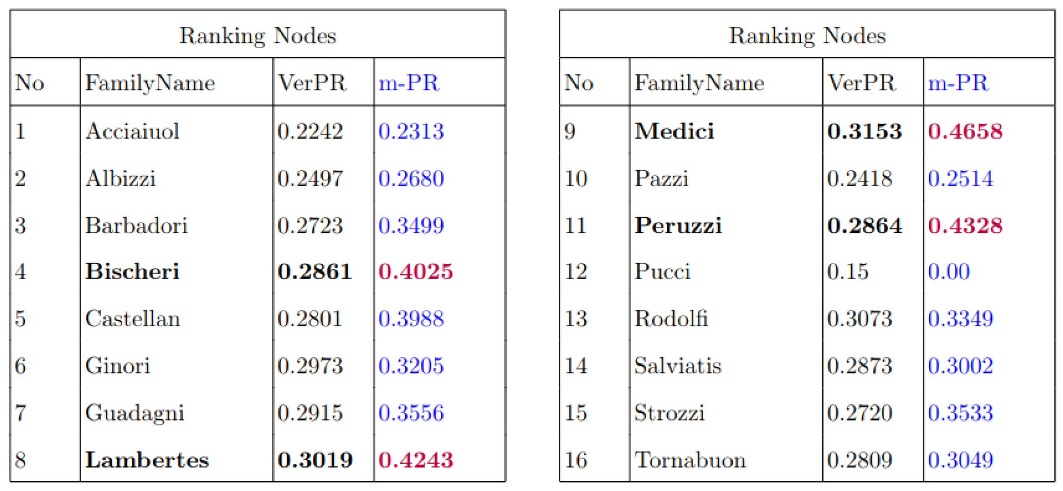
This normalization ensures that the layer weights collectively form a valid probability distribution, reflecting the influence or importance of nodes within the layer l. The goal is to maintain the probability interpretation of rank, where the sum of probabilities within a layer equals 1. This iterative process is continued for all layers and nodes until the rank values converge. The nodes with higher rank scores are considered more influential in the network. Based on a user-specified threshold, the top influencers are selected. For referral convenience, from here on, the proposed approach of influencer identification is referred to as mpr. As a case study, apply the algorithm on the Florentine Family Marriage and Business Ties Data [45], a multilayer network formed with 16 nodes as shown in Figure 3. The Algorithm 1 illustrates the computation of the node rank in a multilayer network. The node ranks are computed for each node. Comparing the ground truth (VerPR), the ranking has improved, and the following observations were made:
- Since node 12 is not linked to any other family in the layer, the computation is performed by taking out this node from the whole network.
- The most important node is node 9, corresponding to the Medici family (shown in Figure 3).
- The effective choice of individualization factors for each layer greatly improves ranking optimization, thus affirming the credibility of m-PageRank (shown in Figure 3).
Iterative convergence of rank value involves comparing the new PageRank scores with the previous ones that considered connections from the same layer connections and from different layers connections. Thus, the update phase involves connections and time for convergence checking.
| Algorithm 1 Influencers’ Identification in Multilayer Network |
|
Input: , Output:
|
Figure 2.
Layers of Florentine family business (left) and family marriage relations (right).
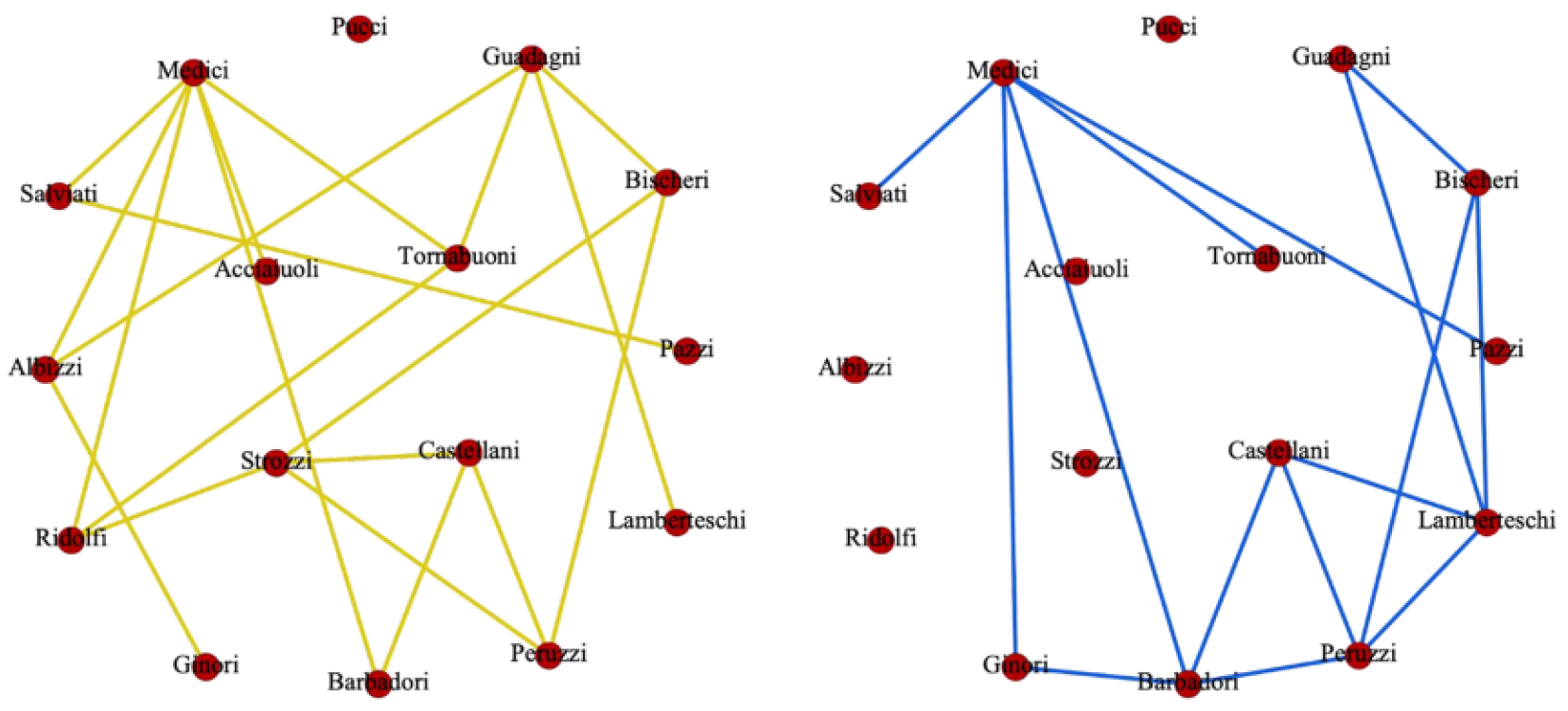
Figure 3.
Tabulation of ranks of nodes using Ver-PR and m-PR.
3.2. Formation of Block around the Influencer
Once the influencers are identified, the next goal is to build blocks around each of them. The nodes within the blocks are determined by their affinity for the influencers. The affinity is computed based on the strongest properties that the nodes share with the influencers. A node may thus become part of one or more blocks, resulting in overlapping blocks. Nodes with no affinity for the influencer may not be part of any block. This means that these nodes may not contribute to link prediction at this time. Since the influencers were identified across the layers, the distinguishing aspect of our block formation technique centred around the influencer captures and preserves the interplay between the layers.
- How strongly the node is connected to its neighbors in the network. Through this, the local importance of the network is uncovered.
- How similar are the nodes based on attributes and interactions, thereby uncovering the network’s structure.
These blocks offer a higher level of abstraction than individual nodes, as they group together nodes with similar connectivity patterns. By considering these blocks alongside individual nodes, link prediction algorithms can better capture the underlying structure of the network and achieve more accurate predictions.
Let v be a neighbor of an influencer I. We want to know if v should be added in the block around I. The more strongly v is connected to its neighbors, the stronger is its local importance. This local importance is defined in terms of the connections that v has with its neighbors. Let neigh(v) denote the set of neighbors {u1, u2, ...} of v. It is easy to see that the strongest connection exists if {u1, u2, ...} ∪ {v} is maximally connected. In other words, the nodes form a complete subgraph, which essentially works out to edges between them. However, the actual number of connections between {u1, u2, ...} ∪ {v} need not reach this maximum. The ratio of the actual number of connections to the maximum number of connections provides a measure of v’s local importance. Let denote the actual connections that {u1, u2, ...} share among themselves, and is the degree of v. Thus, the ratio is the clustering coefficient, given by the formula
The algorithm for computing the correlation is elaborated in Algorithm 2.
| Algorithm 2 Compute Correlation |
|
Input: v, , , , , Output: Correlation for each
|
The node centrality, degree, and clustering coefficient to select similar nodes based on the attributes are considered. Nodes with high centrality act as bridges, connecting different parts of the network, and serve as hubs with many connections. This structural importance helps identify the similarity with the influencer. The degree of the node quantifies the number of edges incident to a node, indicating local prominence within the network. Thus, selecting similar nodes based on attributes (correlation) is a cumulative measure of the degree of node , centrality , clustering coefficients , and and as normalizing factors. The correlation is computed as:
Thus, A block is defined as followed:
Definition 4.
Let be the multilayer network. A block B consisting of nodes such that is built around the influencer I, and has a high clustering coefficient with I and shares similar connectivity patterns within the network.
Thus, block formation is summarized as a three-step process:
- Pick an influencer, I.
- Among all the neighboring nodes of I, we determined a node v that exhibits the strongest local property
- Next, for all neighbors of v, compute the correlation with I.
The formation of blocks surrounding the influential nodes enables the capture of the influence on the overall network structure and modularity. Each block is distinguished by a unique property. Thus, the nodes within a block exhibit more similar properties. Such blocks effectively capture the directed relationships. Since a block consists of nodes distributed across the layers, the interlayer dependency is well preserved by considering the layer information [46]. The blocks ensure the capture of both global and local information relevant to link prediction and information diffusion. Therefore the link prediction between the blocks represents the prediction of the future links between the nodes that exhibit dissimilar characteristics. The information spread in the blocks evaluates how the spread of rumors can be regulated within blocks. The blocks, centered on influencers, also account for the information flow from influential nodes to their neighbors, which is used for both link prediction and information diffusion. This process is elaborated in Algorithm 3.
| Algorithm 3 Block Formation around Influencers |
|
Input: , I (Set of Influencers), Desired Number of Blocks: N Output: Block Set B
|
3.3. Link Prediction between the Blocks
The future links between two blocks depends on the strength of the interconnections between the overall nodes of one block and the overall nodes of another block. The strength is highest when every node of one block connects to every node of the other block. Since the underlying network is a directed network, the strength of the interconnection has both magnitude and direction.
Once the blocks are formed, we use the binomial distribution for likelihood estimation in link prediction, which is rooted in the assumption that the presence or absence of links between nodes follows a binary outcome (link or no link) and that these outcomes are independent across different pairs of nodes. Therefore, the Probability Mass Function (PMF) gives the
where:
- -
- X is the number of observed links between nodes in different blocks,
- -
- is the total number of possible links between nodes in different block i and block j,
- -
- is the number of observed links,
- -
- is the probability of a link between nodes in different block i and block j, calculated based on the likelihood.
Now compute the maximum likelihood with every pair of blocks using the probability mass function (PMF) equation as
where: is the combined likelihood,
and is the observed and total possible connections,
is the strength of the connections, and is the probability mass function. Algorithm 4 elaborates the link prediction process using maximum likelihood estimation.
| Algorithm 4 Link prediction between the blocks |
|
Input: Blocks ; ; threshold: ; Output: probability values;
|
Section 5.1 will demonstrate experimental proof for the block formation and the link prediction process between the blocks on three different dataset.
3.4. Information Dissemination
For the spread of information across the network, the Linear Threshold Model (LTM) is considered as the underlying diffusion model. In LTM, individuals have a specific threshold or required number of neighbors that need to adopt the behavior or innovation before they adopt it. The model assumes that individuals are influenced by their social connections and the behavior of their neighbors, and the adoption process takes place gradually over time [47,48]. In the Linear Threshold Model, the adoption of threshold remains fixed for each individual. This means the model doesn’t account for the individual’s evolving beliefs or changing social context. Once the threshold is crossed, the individual adopts the information, and this decision remains constant throughout the simulation. In reality, the individual’s threshold may dynamically adjust. For instance, exposure to multiple sources of information demands alignment with their evolving beliefs, or changes in the opinions of their social connections could lead to a change in threshold. Thus a node becomes active if the fraction of its active neighbors exceeds a certain threshold.
Let be the different blocks formed around the influencers. Let be the activation probability function for a node n within a block formed. The activation probability can be represented as,
where X denotes the node being in the aware state, Y denotes the size of the cluster, denotes the centrality of the node. The activation probability increases with node centrality and awareness.
Each node in the network is associated with an awareness level, representing the amount of information they have acquired about the topic being spread. This awareness level can vary from node to node. The spread of information occurs through interactions between nodes in the network. Nodes with higher awareness levels are more likely to influence their neighbors and propagate the information further. Nodes may have different thresholds for adopting or transmitting information based on their awareness levels. For example, a node with low awareness may require more exposure to the information before adopting it, while a node with high awareness may quickly adopt and transmit the information.
The normalization factors ensure that the result is in a meaningful range of {0, 1} [49]. The generating function for activation probability within a block represents the probability distribution of the number of nodes activated within the block. Let be a variable related to the activation probability of node within block . The generating function for diffusion within block is computed as [50],
where represents the probability that there are k activated nodes within block and variable capturing the activation probability within block .
Considering the be the different blocks formed around the set of influencers nodes, we can extend this approach to define activation probabilities and generate functions for each block. The overall generating function for the entire multilayer network can then be expressed as a combination of the individual generating functions for each block as,
By focusing on each block individually, we compute the activation probability function according to the specific characteristics and dynamics within the block. Modeling diffusion within each block individually recognizes and accounts for the variations in activation probability across blocks. Considering each block in isolation enables the inclusion of block-specific factors in the activation probability function. The Algorithm 5 illustrates the same.
| Algorithm 5 Activation Probability and Generating Function for Blocks in a Multilayer Network |
|
The analysis of the speed and extent of information dissemination in a network is contingent upon understanding of the spread rate. The spread rate is defined as the rate at which the influence propagates through the network, measured as the number of new activations per unit of time. Thus, we calculate the spread rate through the nodes within the block using the activation probability as
4. Experimental Study and Discussion
The experimental setup progresses with identifying the influencers from the heterogeneous networks and the formation of blocks around the influencers. As discussed, the experimentation progresses with validation of the block formation in two major contexts of research, namely Information spread and Link prediction. We demonstrate two case studies, each related to information spread using block formulation and Link prediction among blocks in heterogeneous complex networks, to validate
- The link prediction between the blocks compared to the current state-of-the-art.
- The information spreads within a block compared against the non-block network, especially during the spread of rumors.
4.1. Analysis of Link Prediction between the Blocks
The future links between two blocks depend on the strength of the interconnections between the overall nodes of one block and the overall nodes of another block. The strength is highest when every node of one block connects to every node of the other block. Since the underlying network is a directed network, the strength of the interconnection has both magnitude and direction. The analysis of the speed and extent of information dissemination in a network is contingent upon understanding of the spread rate. The spread rate is defined as the rate at which the influence propagates through the network, measured as the number of new activations per unit of time. Thus, we calculate the spread rate through the nodes within the block using the activation probability as
5. Experimental Study and Discussion
The experimental setup progresses with identifying the influencers from the heterogeneous networks and the formation of blocks around the influencers. As discussed, the experimentation progresses with validation of the block formation in two major contexts of research, namely Information spread and Link prediction. We demonstrate two case studies, each related to information spread using block formulation and Link prediction among blocks in heterogeneous complex networks, to validate
- The link prediction between the blocks compared to the current state-of-the-art.
- The information spreads within a block compared against the non-block network, especially during the spread of rumors.
5.1. Analysis of Link Prediction between the Blocks
The future links between two blocks depend on the strength of the interconnections between the overall nodes of one block and the overall nodes of another block. The strength is highest when every node of one block connects to every node of the other block. Since the underlying network is a directed network, the strength of the interconnection has both magnitude and direction. The different flavors of complex network datasets from the social, biological, and ecological domains to cover different sets of characteristics are considered. Social datasets usually exhibit dense and balanced characteristics. The Biological dataset, on the other hand, is less dense and slightly imbalanced. The Ecological dataset often exhibits sparse and imbalanced characteristics. Density indicates more information flow and balance implies even density across the network. Both these characteristics affect the link prediction. Table 6 summarises the datasets’ details.
5.1.1. Identifying Influencers
The experimentation is initiated by identifying the influencers and forming the block around them. We start by identifying the rank of the nodes from the multilayer networks. The average rank value for the nodes in a network converges to 1. We pick those nodes exhibiting higher rank value manually until there is a sudden dip in their value, and categorize them as influencers. This is done using the Steps of Algorithm 1. Table 2 shows top influencers along with the rank values of the nodes and the layers computed out of the dataset.
5.1.2. Building the Blocks
For the block formation, we use the clustering coefficient using the Equation 4 to find the nodes v that have the strongest local property among all the influencers’ neighbors, . For all , we compute the correlation with the influencers using the equation 5. For the experimental setup, the adjustable parameters were assigned values of and , respectively. Using as a threshold focuses on strong positive relationships, while filters out weak or negative relationships. We continue the same process with other nodes that are neighbors of the influencers, thus forming the blocks as discussed in steps of Algorithm 3. Table 3 exhibits a snapshot of the blocks formed around the influencers and their size, which forms the basis for interblock link prediction.
5.1.3. Link Prediction between the Blocks
Once the blocks are formed, the next step is to predict the links between the blocks using the Algorithm 4. Table 4 exhibits the probability of future links. The block-based approach to predict the links between the blocks exploited block structure and the strength of the relationships between dissimilar block pairs by extracting insights into the network structures, nature of the links, and heterogeneity information and aggregating them at the block level, thus reducing the computational complexity to polynomial time, making it suitable to scale large networks. The higher the probability values, the higher the chances of future link occurrences.
The proposed method of link prediction between the blocks is evaluated for its efficacy. To this end, we removed of the existing links arbitrarily from the network and assessed how the model predicted these removed links. This is a standard approach adopted for link prediction in the literature. Our first goal in measuring efficacy is the model’s correctness. Therefore, we use Accuracy as a metric. However, accuracy fails for unbalanced datasets and is not sufficient for all scenarios. Precision focuses on the positive predictions’ reliability and, hence, can handle imbalances in the dataset. The AUC-ROC is used to distinguish between positive and negative links across various threshold settings. Our approach is compared against non-block-based link prediction. Table 5 compares the results of the accuracy of link prediction with our block-based approach over the non block approach.
5.1.4. Observations
The block-to-block approach exploited the block structure and the strength of the relationships between dissimilar block pairs by extracting insights into the network structures, nature of the links, and heterogeneity information and aggregating them at the block level, thus reducing the computational complexity to polynomial time, making it suitable to scale large networks. The results demonstrate the capability to identify numerous potential links through block modeling that other methods could not detect. It is observed that the network’s structure and dynamics are crucial in the link prediction process.
5.1.5. Evaluation
The proposed approach is compared against the current state of the art using Accuracy, Precision and AUC- ROC curve. It is observed that block-to-block link prediction could predict the links between the dissimilar nodes nearly more accurately compared to the link prediction approach that considered the entire network. This is tabulated in Table 5. To summarize, a close connection between the block-block link prediction and the likelihood estimation is established based on a binomial distribution. This allowed us to draw upon the maximum likelihood estimation to predict future links. The block model served as a strong foundation to build the probabilistic model for inter-block-based link prediction. This approach is a hybrid approach, considering the global and local significance and the directionality aspect of the network. Other hybrid approaches are restricted only to similarity-based techniques, while our approach exploits network structures, directionality, heterogeneity and builds a probabilistic model for predicting the directed links more accurately.

Table 5.
Comparison of block-to-block link prediction with non-block network.
| Block to Block Link prediction | Without Block Model | ||||
|---|---|---|---|---|---|
| # | Datasets | Accuracy | Precision | Recall | Accuracy |
| 1 | SNAP College MSG | 0.942 | 0.91 | 0.893 | 0.502 |
| 2 | Arabidopsis Genetic | 0.901 | 0.891 | 0.912 | 0.537 |
| 3 | Alaska Venetie | 0.743 | 0.886 | 0.897 | 0.352 |
| 4 | Alaska Wainwright | 0.758 | 0.876 | 0.896 | 0.302 |
| 5 | Alaska Katkovi | 0.713 | 0.884 | 0.892 | 0.283 |
5.2. Analysis of Information Diffusion Using Blocks
5.2.1. Dataset
Two different multilayer datasets, whose details are illustrated in Table 6 are used for analysis of information spread in the network.
- -
- Higgs multiplex: The Higgs dataset, built from Twitter by observing the spreading process on 4th July 2012 [51]. The spreading process is observed before, during, and after the diffusion. The dataset contains 456626 nodes and 14855842 edges. It is a two-layer network. The layers capture the interactions on Twitter and correspond to the different actions taking place in the social networks. The data format is userA userB timestamp interaction, and both layers use the same nodeID.
- -
- Citation-network: The dataset consists of citation data from indexing databases such as DBLP, ACM, MAG (Microsoft Academic Graph) [52]. The dataset consists of 629,814 articles and 632,752 citations.
Table 6.
Summary of Dataset for Information Diffusion.
| Networks | Vertices | Edges | Layers |
|---|---|---|---|
| DBLP | 12600 | 49700 | 4 |
| HIGGS | 302975 | 449827 | 2 |
5.2.2. Identifying the Influencers
As discussed, the influencers are identified from the network using the Algorithm 1 as shown in Table 7. The blocks are formed around the influencers using the Algorithm 3. The nodes exhibiting higher affinity towards the influencer are added into a block. The blocks thus formed along with the size are illustrated in Table 8.
5.2.3. Observation
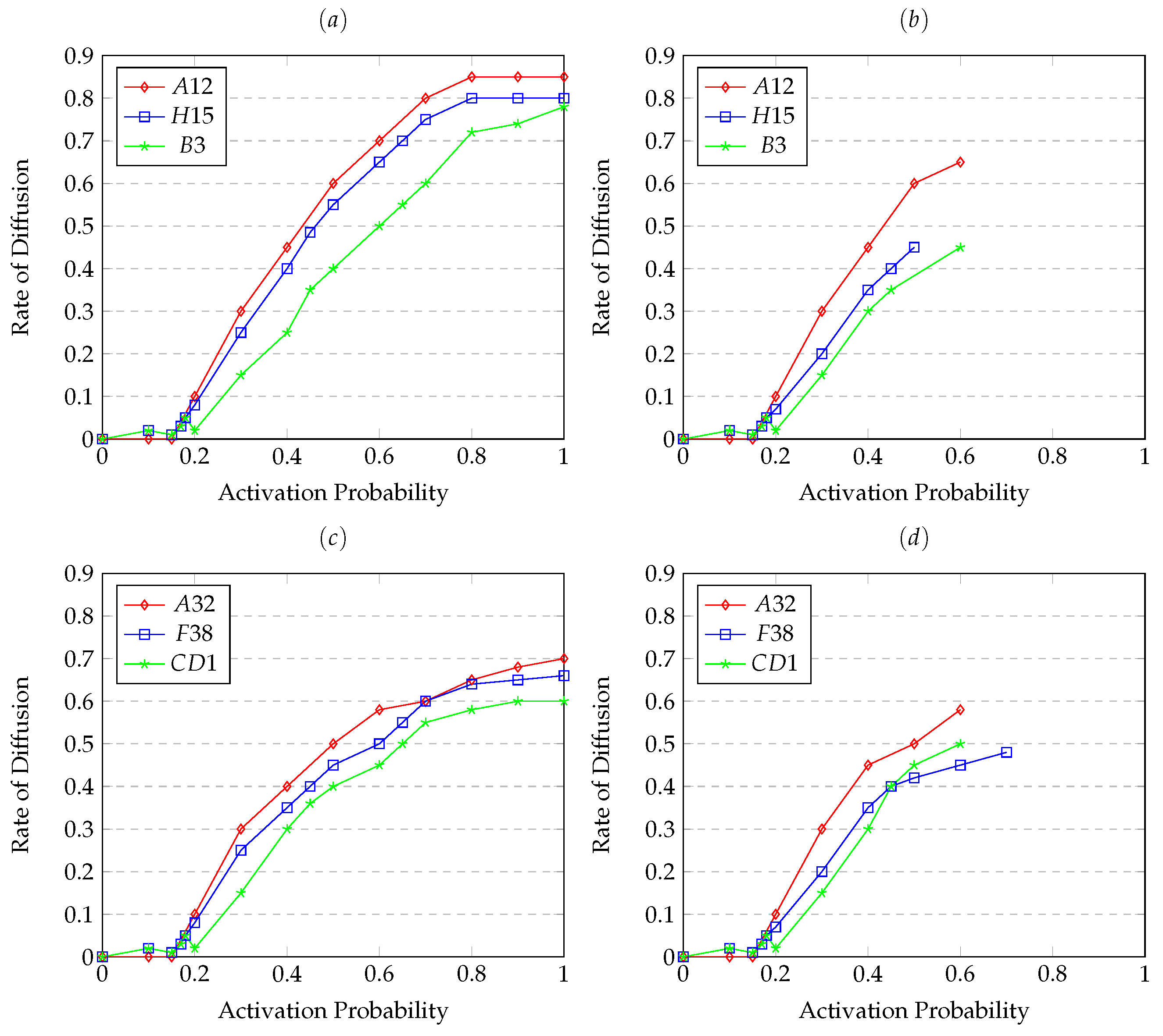
To measure the extent of information spreading, we tracked the number of influenced nodes, observed the spread of influence over time. By calculating the spread rate, which involved dividing the number of influenced nodes by the network volume, we could quantify the speed at which information spread. The detailed spread rate, the speed at which information reaches the entire network, and the time required for convergence for the selected network with different seed(k) are computed and tabulated, and the same is shown in Table 9.
Figure 4.
The diffusion analysis corresponds to Single and Triangle Edge with in cluster. (a) Higgs multiplex having Single Edge with in cluster, (b) Higgs multiplex having triangle Edge with in cluster, (c) Citation Networks having Single Edge with in cluster, (d) Citation Networks having triangle Edge with in cluster.
The efficacy of the block model for information spread is compared against the network with blocks (NB) and network without any blocks (NN). The presence of blocks significantly impacts the pace of diffusion in networks, particularly concerning epidemic propagation. These coefficients measure the level of clustering within a network and directly influence diffusion rates. Block formation in network facilitates or hinders epidemic spread, depending on variables like transmission dynamics and network configuration. Block formation across multiple layers affects diffusion by accounting for interactions among these layers, wherein the formation of clusters of interconnected nodes plays a pivotal role in shaping the speed and extent of diffusion across the network. Figure 5 exhibits the diffusion rate in a network with blocks spread between layers and non-block networks. We observe that the diffusion rate is higher in the non-block network for both datasets under comparison.
6. Conclusion and Future Scope
In this study, we presented a novel approach to identify the influencers in a directed heterogeneous multilayer network. Our approach of identifying the influencers ensured interlayer similarity and layer weightage, as opposed to the current state-of-the-art of finding the influencers in the network. The influencers thus identified formed the basis for the novel block formation algorithm that resulted in the blocks. The blocks took into account multiple characteristics, allowing us to seamlessly integrate the information from various layers. We then progressed with the block analysis by addressing the link prediction and the information dissemination through these blocks. Unlike other techniques that use layer- or attribute-based metrics, the block-based approach is superior because it combines the information from multiple layers, interplay between layers, and dominant attributes. The utilization of the layer weight and the node rank information, enhanced the prospect of finding the "real" influencers with a reduced computational complexity of . The ability of the block formation algorithm to capture the heterogeneity of nodes at the edge and the layer level helped in predicting links that otherwise could have gone unnoticed between the dissimilar nodes. The findings also reveal that the blocks hinder information dissemination and reduce spread volume, particularly in the context of epidemic spread. These findings provide valuable insights into the complex dynamics of information diffusion and link prediction in heterogeneous networks.
References
- Kivelä, M.; Arenas, A.; Barthelemy, M.; Gleeson, J.P.; Moreno, Y.; Porter, M.A. Multilayer networks. Journal of complex networks 2014, 2, 203–271. [CrossRef]
- Swain, D.; Eesha, S.; Raj, G.D.; Anjali, T. A Novel Architecture for Community Detection Between Large Social Media Creators. Procedia Computer Science 2024, 233, 87–96. [CrossRef]
- Deepthi, L.; others. Link Prediction in Citation Networks: A Survey. 2022 Third International Conference on Intelligent Computing Instrumentation and Control Technologies (ICICICT). IEEE, 2022, pp. 1194–1200. [CrossRef]
- Nair, A.; Harikumar, G.; Vissutha, M.; Ajanalakshmi, D.; Deepthi, L. Classification of Trust in Social Networks using Machine Learning Algorithms. 2022 Third International Conference on Intelligent Computing Instrumentation and Control Technologies (ICICICT). IEEE, 2022, pp. 501–505. [CrossRef]
- Huberman, B.A.; Adamic, L.A. Growth dynamics of the world-wide web. Nature 1999, 401, 131–131. [CrossRef]
- Albert, R.; Jeong, H.; Barabási, A.L. Diameter of the world-wide web. nature 1999, 401, 130–131. [CrossRef]
- Newman, M.E.; Park, J. Why social networks are different from other types of networks. Physical review E 2003, 68, 036122. [CrossRef]
- Nair, L.S.; Cheriyan, J.; Swaminathan, J. Microscopic structural analysis of complex networks: An empirical study using motifs. IEEE Access 2022, 10, 33220–33229. [CrossRef]
- Freeman, L.C.; others. Centrality in social networks: Conceptual clarification. Social network: critical concepts in sociology. Londres: Routledge 2002, 1, 238–263. [CrossRef]
- Van Steen, M. Graph theory and complex networks. An introduction 2010, 144.
- Zhang, J.; Luo, Y. Degree centrality, betweenness centrality, and closeness centrality in social network. 2017 2nd international conference on modelling, simulation and applied mathematics (MSAM2017). Atlantis press, 2017, pp. 300–303. [CrossRef]
- Kim, D.Y. Closeness centrality: A social network perspective. Journal of International & Interdisciplinary Business Research 2019, 6, 115–122. [CrossRef]
- Okamoto, K.; Chen, W.; Li, X.Y. Ranking of closeness centrality for large-scale social networks. International workshop on frontiers in algorithmics. Springer, 2008, pp. 186–195. [CrossRef]
- Negre, C.F.; Morzan, U.N.; Hendrickson, H.P.; Pal, R.; Lisi, G.P.; Loria, J.P.; Rivalta, I.; Ho, J.; Batista, V.S. Eigenvector centrality for characterization of protein allosteric pathways. Proceedings of the National Academy of Sciences 2018, 115, E12201–E12208. [CrossRef]
- Hurtgen, M.; Praks, P.; Zajac, P.; Maun, J.C. Comparison of measurement placement algorithms for state estimation based on theoretic and eigenvector centrality procedures. Power Systems Computation Conference, 2008.
- Page, L.; Brin, S.; Motwani, R.; Winograd, T. The PageRank citation ranking: Bringing order to the web. Technical report, Stanford infolab, 1999.
- Pant, B.; Ramirez, R.; Reeves, L. Google PageRank explained via power iteration 2019.
- Bonacich, P. Power and centrality: A family of measures. American journal of sociology 1987, 92, 1170–1182. [CrossRef]
- Brandes, U. A faster algorithm for betweenness centrality. Journal of mathematical sociology 2001, 25, 163–177. [CrossRef]
- Brin, S. The PageRank citation ranking: bringing order to the web. Proceedings of ASIS, 1998 1998, 98, 161–172.
- Boldi, P.; Vigna, S. The webgraph framework I: compression techniques. Proceedings of the 13th international conference on World Wide Web, 2004, pp. 595–602. [CrossRef]
- Newman, M.E. A measure of betweenness centrality based on random walks. Social networks 2005, 27, 39–54. [CrossRef]
- Wang, Z.; Wang, L.; Perc, M. Degree mixing in multilayer networks impedes the evolution of cooperation. Physical Review E 2014, 89, 052813. [CrossRef]
- Bródka, P.; Skibicki, K.; Kazienko, P.; Musiał, K. A degree centrality in multi-layered social network. 2011 international conference on computational aspects of social networks (CASoN). IEEE, 2011, pp. 237–242. [CrossRef]
- Basaras, P.; Iosifidis, G.; Katsaros, D.; Tassiulas, L. Identifying influential spreaders in complex multilayer networks: A centrality perspective. IEEE Transactions on Network Science and Engineering 2017, 6, 31–45. [CrossRef]
- De Domenico, M.; Solé-Ribalta, A.; Omodei, E.; Gómez, S.; Arenas, A. Ranking in interconnected multilayer networks reveals versatile nodes. Nature communications 2015, 6, 6868. [CrossRef]
- Chen, X.; Lu, Z.M. Measure of layer centrality in multilayer network. International Journal of Modern Physics C 2018, 29, 1850051. [CrossRef]
- Lee, K.M.; Min, B.; Goh, K.I. Towards real-world complexity: an introduction to multiplex networks. The European Physical Journal B 2015, 88, 1–20. [CrossRef]
- Solé-Ribalta, A.; De Domenico, M.; Gómez, S.; Arenas, A. Centrality rankings in multiplex networks. Proceedings of the 2014 ACM conference on Web science, 2014, pp. 149–155. [CrossRef]
- Solé-Ribalta, A.; De Domenico, M.; Gómez, S.; Arenas, A. Random walk centrality in interconnected multilayer networks. Physica D: Nonlinear Phenomena 2016, 323, 73–79. [CrossRef]
- Rocha, L.E.; Masuda, N. Random walk centrality for temporal networks. New Journal of Physics 2014, 16, 063023. [CrossRef]
- Noh, J.D.; Rieger, H. Random walks on complex networks. Physical review letters 2004, 92, 118701. [CrossRef]
- Wąs, T.; Rahwan, T.; Skibski, O. Random walk decay centrality. Proceedings of the AAAI Conference on Artificial Intelligence, 2019, Vol. 33, pp. 2197–2204. [CrossRef]
- Xie, J.; Kelley, S.; Szymanski, B.K. Overlapping community detection in networks: The state-of-the-art and comparative study. Acm computing surveys (csur) 2013, 45, 1–35. [CrossRef]
- Papakostas, D.; Basaras, P.; Katsaros, D.; Tassiulas, L. Backbone formation in military multi-layer ad hoc networks using complex network concepts. MILCOM 2016-2016 IEEE Military Communications Conference. IEEE, 2016, pp. 842–848. [CrossRef]
- Gao, Z.K.; Dang, W.D.; Li, S.; Yang, Y.X.; Wang, H.T.; Sheng, J.R.; Wang, X.F. PageRank versatility analysis of multilayer modality-based network for exploring the evolution of oil-water slug flow. Scientific Reports 2017, 7, 5493. [CrossRef]
- Halu, A.; Mondragón, R.J.; Panzarasa, P.; Bianconi, G. Multiplex pagerank. PloS one 2013, 8, e78293. [CrossRef]
- Kitsak, M.; Gallos, L.K.; Havlin, S.; Liljeros, F.; Muchnik, L.; Stanley, H.E.; Makse, H.A. Identification of influential spreaders in complex networks. Nature physics 2010, 6, 888–893. [CrossRef]
- Pei, S.; Muchnik, L.; Andrade, Jr, J.S.; Zheng, Z.; Makse, H.A. Searching for superspreaders of information in real-world social media. Scientific reports 2014, 4, 5547. [CrossRef]
- Leskovec, J.; Adamic, L.A.; Huberman, B.A. The dynamics of viral marketing. ACM Transactions on the Web (TWEB) 2007, 1, 5–es. [CrossRef]
- Poux-Médard, G.; Pastor-Satorras, R.; Castellano, C. Influential spreaders for recurrent epidemics on networks. Physical Review Research 2020, 2, 023332. [CrossRef]
- Bauer, F.; Lizier, J.T. Identifying influential spreaders and efficiently estimating infection numbers in epidemic models: A walk counting approach. Europhysics Letters 2012, 99, 68007. [CrossRef]
- Kempe, D.; Kleinberg, J.; Tardos, É. Maximizing the spread of influence through a social network. Proceedings of the ninth ACM SIGKDD international conference on Knowledge discovery and data mining, 2003, pp. 137–146. [CrossRef]
- Cheriyan, J.; Sajeev, G. m-PageRank: A novel centrality measure for multilayer networks. Advances in Complex Systems 2020, 23, 2050012. [CrossRef]
- Prajda, K. Unions of Interest. Florentine Marriage Ties and Business Networks in the Kingdom of Hungary during the Reign of Sigismund of Luxemburg 2012.
- Nair, L.S.; Jayaraman, S.; Krishna Nagam, S.P. An improved link prediction approach for directed complex networks using stochastic block modeling. Big Data and Cognitive Computing 2023, 7, 31. [CrossRef]
- Zhang, Z.K.; Liu, C.; Zhan, X.X.; Lu, X.; Zhang, C.X.; Zhang, Y.C. Dynamics of information diffusion and its applications on complex networks. Physics Reports 2016, 651, 1–34. [CrossRef]
- Cheriyan, J.; Nair, J.J. Influence Minimization With Node Surveillance in Online Social Networks. IEEE Access 2022, 10, 103610–103618. doi:10.1109/ACCESS.2022.3210126. [CrossRef]
- Zhang, J.; Fang, Z.; Chen, W.; Tang, J. Diffusion of “following” links in microblogging networks. IEEE Transactions on Knowledge and Data Engineering 2015, 27, 2093–2106. [CrossRef]
- Granovetter, M. Threshold models of collective behavior. American journal of sociology 1978, 83, 1420–1443. [CrossRef]
- https://snap.stanford.edu/data/higgs-twitter.html. Technical report.
- https://www.aminer.org/citation. Technical report.
Figure 5.
The relationship between Block size and diffusion rate.
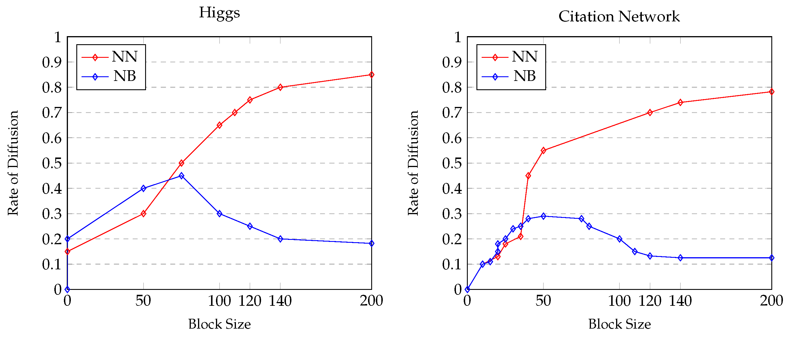
Table 1.
Literature review of centrality metrics for multilayer networks.
| Centrality metric | Method | Limitations |
| Random walk centrality 2016 | Mean First | Limited to Technology Networks, |
| Random-walk BC | Passage Time (MFPT) | and static networks |
| Random-walk CC | ||
| Power Community Index(PCI) 2017 | Centrality Perspective | Refrains from considering |
| -PCI, al-PCI | using connection | the entire network topology |
| ml-PCI, ls-PCI | (Degree of node) | Limited to scaling |
| Multiplex PageRank 2018 | All layers treated as | Applied to |
| (additive PR(addPR) | single layer logically | Multiplex Networks |
| multiplicative PR(mulPR) | (Individual Ranks add/mul together) | with duplex mode |
| PageRank versatility 2019 | Personalized Vector added | Defined for |
| Versatile BC | ( vector formation | Multiplex Networks |
| depends on type of networks) | (Technology Networks) |
Table 2.
Snapshots of a few influencers identified from the datasets.
| Coll-Msg | Arabidopsis | Venetie | Wainwright | Kaktovi |
|---|---|---|---|---|
| 57.901003 | 301.720895 | 2.36527 | 6.432528 | 4.2054 |
| 57.835896 | 52.246835 | 2.287706 | 5.601206 | 3.373879 |
| 48.207632 | 50.270275 | 2.228333 | 5.066489 | 3.298377 |
| 41.603781 | 46.246756 | 2.160444 | 4.502255 | 3.014692 |
| 39.662304 | 42.390381 | 2.002166 | 4.274835 | 2.791716 |
Table 3.
Five blocks formed and its sizes in multilayer networks.
| SNAP | Arabidopsis | Katkovi | Wainwright | Venetie | |||||
|---|---|---|---|---|---|---|---|---|---|
| BlockID | Size | BlockID | Size | BlockID | Size | BlockID | Size | BlockID | Size |
| 42I | 3227 | 33X | 7779 | 73K | 223 | 140A | 129 | 123M | 411 |
| 632A | 54 | 2100X | 16 | 94N | 39 | 141T | 23 | 149J | 36 |
| 393G | 128 | 402A | 7 | 43K | 55 | 133V | 34 | 125T | 119 |
| 402A | 19 | 5X | 171 | 79D | 89 | 98L | 3 | 153O | 6 |
| 728A | 62 | 1176X | 160 | 55V | 12 | 197D | 6 | 86L | 28 |
Table 4.
Predicting the link between the blocks.
| Dataset | |||
|---|---|---|---|
| SNAP College MSG | 494D | 492D | 0.857143 |
| 402A | 400A | 0.666667 | |
| 402A | 431A | 0.5 | |
| 402A | 728A | 0.5 | |
| 402A | 632A | 0.5 | |
| Arabidopsis Genetic Layer | 33X | 5X | 0.425 |
| 2100X | 1577X | 0.543 | |
| 2100X | 5360X | 0.519 | |
| 2100X | 2305X | 0.325 | |
| 2100X | 375X | 0.225 | |
| Alaska Katkovi | 73K | 43K | 0.5333 |
| 73K | 94N | 0.5033 | |
| 73K | 79b | 0.335 | |
| 73K | 55V | 0.3033 | |
| 73K | 45W | 0.234 | |
| Alaska Wainwright | 123I | 133U | 0.55556 |
| 141T | 125V | 0.45455 | |
| 141T | 69Z | 0.27778 | |
| 141T | 198E | 0.27778 | |
| 141T | 178P | 0.27778 | |
| Alaska Venetie | 123m | 137U | 0.5234 |
| 123m | 86l | 0.4142 | |
| 123m | 137d | 0.3891 | |
| 123m | 175J | 0.3185 | |
| 123m | 130J | 0.2582 |
Table 7.
The mPR computation to identify influencer node.
| Dataset | NodeID( | Layer() | mPR() |
|---|---|---|---|
| 24562 | 1.456 | ||
| 125205 | 1.42 | ||
| Higgs | 10030 | 1.378 | |
| 250010 | 1.24 | ||
| ⋮ | ⋮ | ⋮ | |
| 213 | 0.00 | ||
| 354010 | 1.895 | ||
| 302010 | 1.72 | ||
| Citation Networks | 10028 | 1.401 | |
| 512 | 1.400 | ||
| ⋮ | ⋮ | ⋮ | |
| 5120 | 0.002 |
Table 8.
Blocks formed and its sizes in multilayer networks.
| Higgs | Citation | ||
|---|---|---|---|
| BlockID | Size | BlockID | Size |
| A12 | 108 | A32 | 126 |
| B3 | 84 | B4A | 89 |
| H4 | 38 | CD1 | 32 |
| H15 | 102 | F38 | 92 |
| |r|F12 | 40 | GH1 | 42 |
Table 9.
The spread rate and execution time (t) of the algorithm for different dataset with varying seed volume for m-PageRank validation.
Table 9.
The spread rate and execution time (t) of the algorithm for different dataset with varying seed volume for m-PageRank validation.
| Networks | Seed(K) | Iteration | Spreadrate | Time, t |
|---|---|---|---|---|
| DBLP | 25 | 100 | 0.6932 | 52msec |
| DBLP | 50 | 88 | 0.7642 | 44msec |
| DBLP | 80 | 71 | 0.7811 | 41msec |
| DBLP | 120 | 54 | 0.84 | 36msec |
| HIGGS | 25 | 100 | 0.5432 | 114msec |
| HIGGS | 50 | 91 | 0.6420 | 90msec |
| HIGGS | 80 | 74 | 0.7511 | 72msec |
| HIGGS | 120 | 48 | 0.7601 | 65msec |
Disclaimer/Publisher’s Note: The statements, opinions and data contained in all publications are solely those of the individual author(s) and contributor(s) and not of MDPI and/or the editor(s). MDPI and/or the editor(s) disclaim responsibility for any injury to people or property resulting from any ideas, methods, instructions or products referred to in the content. |
© 2024 by the authors. Licensee MDPI, Basel, Switzerland. This article is an open access article distributed under the terms and conditions of the Creative Commons Attribution (CC BY) license (http://creativecommons.org/licenses/by/4.0/).
Copyright: This open access article is published under a Creative Commons CC BY 4.0 license, which permit the free download, distribution, and reuse, provided that the author and preprint are cited in any reuse.


