Investigating The Applicability Of The Peak Density Thickness Parameter Over The Equatorial Region- A One-Day Case Study

Mohamed Shammat; Bodo Reinisch; Ivan Galkin; Philip Erickson; Bill Rideout; Jay Weitzen

doi:10.20944/preprints202408.0037.v1

Submitted:

31 July 2024

Posted:

02 August 2024

You are already at the latest version

Abstract

This research builds on the previously established Peak Density Thickness (PDT) concept for midlatitudes at Millstone Hill by examining its applicability at equatorial latitudes using data from the Jicamarca Incoherent Scatter Radar (ISR) in Lima, Peru. An 18-hour dataset was meticulously analyzed to capture the F2 layer's PDT parameter with high spatial resolution. This study aims to confirm the presence of the PDT phenomenon at equatorial latitudes, utilizing Jicamarca ISR and the co-located Digisonde station. The results indicate that the PDT parameter reaches its peak value around solar noon, consistent with observations at Millstone Hill and high latitudes. Additionally, the Nsumei et al. Vary-Chap topside model was employed to reconstruct the topside ionospheric profile, validating its utility across different latitudes. These findings suggest that incorporating the Peak Density Thickness χ into ionospheric models can enhance the accuracy of topside specifications derived from ground-based ionosonde measurements. This research highlights the significance of the PDT parameter in understanding ionospheric plasma dynamics and improving predictive models of ionospheric behavior.

Keywords:

Ionosphere

;

electron density

;

topside

;

bottomside

;

Incoherent Scatter Radar

;

ionosonde

;

Jicamarca ISR

Subject:

Environmental and Earth Sciences - Atmospheric Science and Meteorology

Introduction

Traditional models of the Earth’s ionosphere, developed from early scientific studies, depict a sharp “pointed peak” of ionized gas density, driven by the interplay between solar radiation and atmospheric density (Fleming, 1902). This representation has been elaborated through various physical (Chapman, 1931) and numerical models (Croft & Hoogansian, 1968). However, recent studies have identified several inconsistencies between this model and observed ionospheric properties.

One major issue is the discrepancies between sub- and super-peak observations of the peak height hmF2. Jackson (1969) pointed out a small gap in the composite profile at hmF2 when comparing satellite data from Alouette II to ground-based observations from Wallops Island Ionosonde (Figure 1). This discrepancy has been largely ignored due to the limited availability of simultaneous measurements from both spaceborne topside and ground-based bottomside ionosondes.

Further investigations into this discrepancy include Nsumei et al. (2010), who conducted a comparative study of monthly median hmF2 values at mid-latitude locations in North America and Europe. Using ISIS-2 topside ionosonde measurements from 1973 to 1983, compared to ground-based ionosonde measurements a decade later, they reported significant disagreements during spring evening hours, a discrepancy that remains unexplained. Additionally, Gulyaeva (1997) noted discrepancies in TEC measurements during ionospheric perturbations compared to predictions from standard electron density models, leading to the hypothesis of an intermediate layer between the ionosphere’s bottomside and topside.

Our previous work introduced the Peak Density Thickness (PDT) concept using Millstone Hill Incoherent Scatter Radar (ISR) measurements to address these discrepancies and improve our understanding of ionospheric plasma profiling. By utilizing ISR measurements (Erickson, 1998, 2012; Evans, 1965) and the availability of open-data from ionosonde and ISR measurements, we conducted a coordinated investigation into peak electron density using simultaneous measurements from the Millstone Hill ISR (MH-ISR) and the collocated Digisonde DPS4D (Reinisch et al., 2009). We also processed a comprehensive set of 88,412 profiles from MH-ISR, spanning from 1993 to 2023, to measure the peak plasma density thickness. These findings represent a significant step forward in resolving unexplained discrepancies and enhancing our understanding of ionospheric plasma dynamics.

Extending the Investigation to Equatorial Latitudes using Jicamarca Incoherent Scatter Radar

Building on the PDT formalism established at Millstone Hill [Shammat et al., 2024], this study explores the Peak Density Thickness (PDT) of the ionosphere using the Jicamarca Incoherent Scatter Radar (ISR) in Lima, Peru. An 18-hour dataset from October 28th, 2021, was meticulously analyzed to capture the F2 layer’s PDT parameter with exceptional spatial resolution. This research aims to verify the presence of the PDT phenomenon at equatorial latitudes, using Jicamarca ISR and the co-located Digisonde station.

The Vary-Chap Topside Profile:

Reinisch et al. [2007] used the general Chapman function [Rishbeth and Garriott, 1969] to develop the “Vary-Chap” profile, which allowed the scale height to continuously vary with height:

(1)

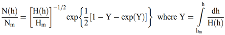
where Nm, Hm, and hm are the density, scale height, and height, respectively, of the F2 layer peak, and H(h) represents the scale height. However, the use of Hm at the F2 peak from the bottomside profile for constructing the topside normalized scale height function H(h)/Hm, as suggested in previous analyses, produced unsatisfactory results [Kutiev et al., 2009].

Nsumei et al. [2012] adopted the same Vary-Chap technique but replaced H(h)/Hm with a shape function S(h) as shown in equation (2):

(2)

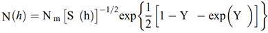
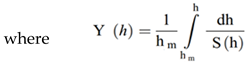
In this study, we adopt the Vary-Chap profile proposed by Nsumei et al. [2012], but instead of setting hm= hmF2 to reconstruct and start the topside profile, we use the sum of the peak height hmF2 and the Peak Density Thickness (PDT) χ. Therefore, h_m= hmF2+ χ and χ represents the Peak Density Thickness (PDT).

Jicamarca ISR Experiment Results

On October 28th, 2021, Jicamarca ISR measurements of the full electron density profile over an 18-hour period were retrieved from the Madrigal database to investigate the existence of the Peak Density Thickness (PDT). Jicamarca ISR profiles predominantly showed a flat F2 peak during a 5-hour window centered around solar noon in Lima at 11:51 am (Figure 8), contrasting with the remaining profiles that depicted a sharply defined F2 peak density. This observation aligns with previous results from MIT Haystack Observatory and Poker Flat ISR, which suggested that the PDT parameter reaches its maximum value around solar noon.

To reconstruct the topside profile, we employed the Vary-Chap topside model proposed by Nsumei et al. (2012). However, rather than starting the profile from hmF2, we began from hmF2+ PDT. The values of the PDT were visually determined to fit the measured ISR profiles. We implemented least square fitting to determine the values of the Vary-Chap parameters α, β, and the transition height hT to match the measured ISR topside profiles. The reconstructed Vary-Chap topside profile closely aligned with the measured ISR profile for most of the time, except during significant density perturbations at higher altitudes (see Figure 5).

Figure 1. Comparison of Ionospheric Electron Density Profiles: Data collected on September 11, 1966, at Wallops Island, VA, show upward measurements from the Wallops Island Ionosonde at 15:45 GMT (Ord. Trace 1545) and downward measurements from the Alouette II satellite at 15:51 GMT (AL-2 at 520 km, Ord. Trace 155056). A discrepancy of approximately 20 km in the hmF2 altitude is noted. The ordinary (Ord.) and extraordinary (Ext.) mode traces, influenced by the Earth’s magnetic field, are indicated (Adapted from Jackson, 1969).

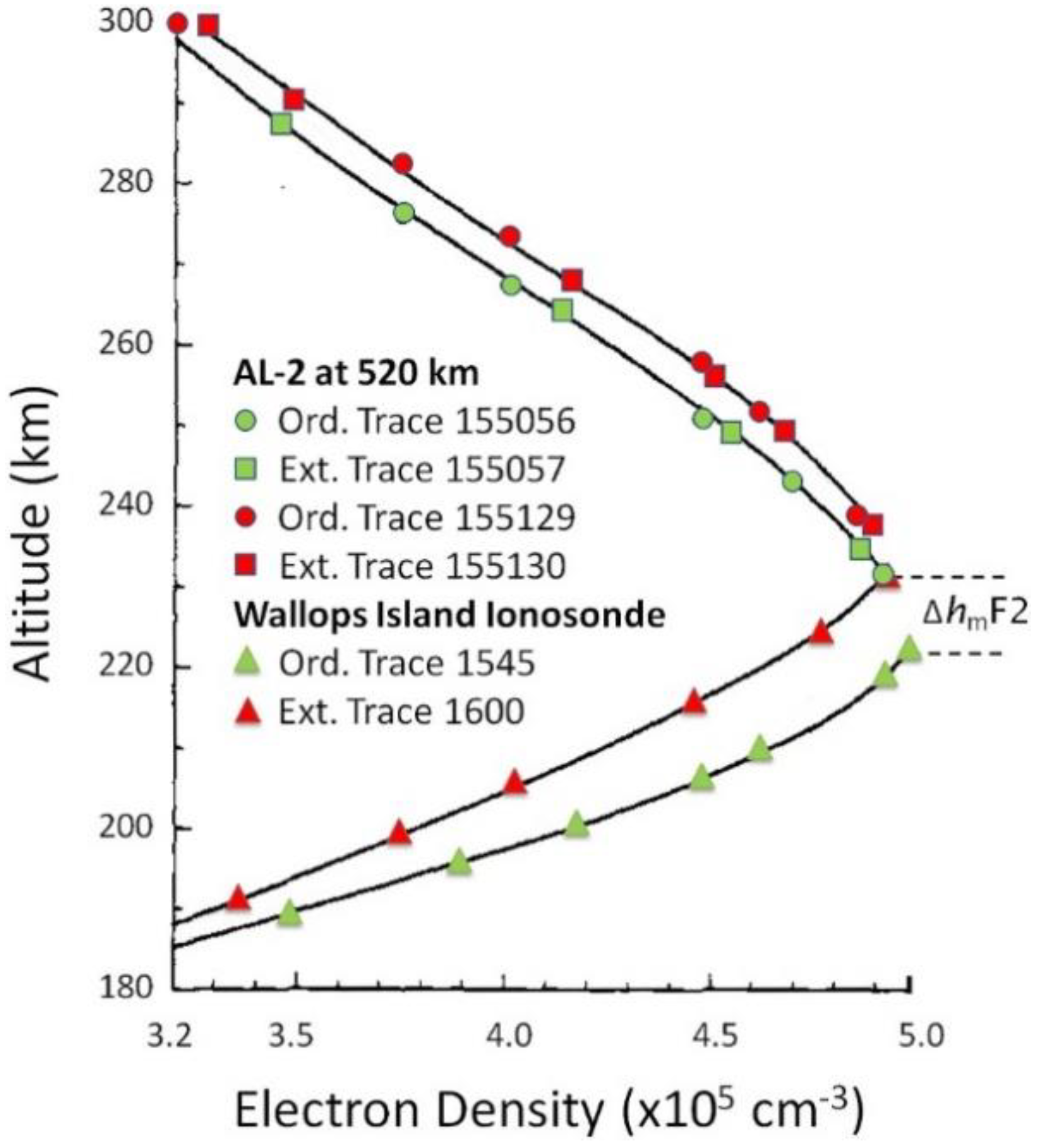
Figure 2. The combined ionosonde-derived (blue circles) and Incoherent Scatter Radar (ISR)-derived (red squares) measurements illustrate a flat F2 peak with a Peak Density Thickness (χ) of 36 km. In this particular example, the F2 peak heights differ significantly between the Digisonde and ISR measurements; hmF2ISR is obtained from ISR, while hmF2Digi is obtained from the Digisonde (in this paper, hmF2 without a subscript refers to hmF2Digi) (adapted from Shammat et al., 2024).

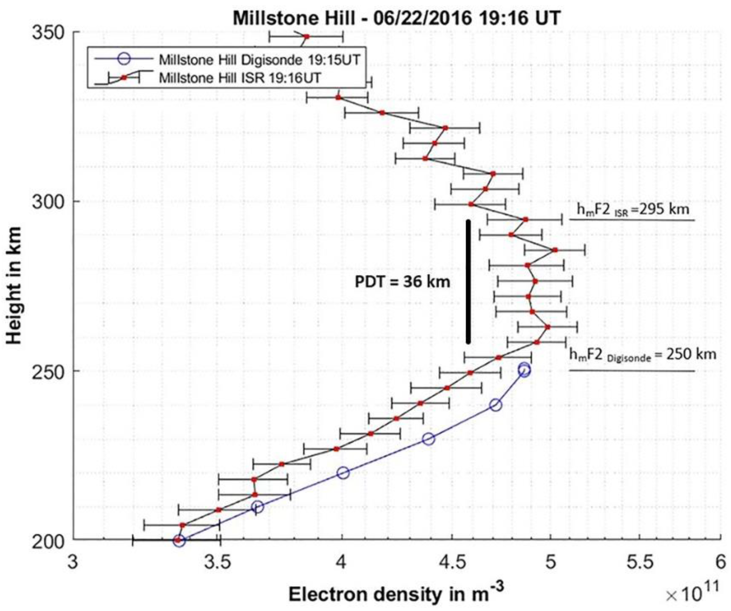
Figure 3. This figure illustrates the yearly distribution of the 88,412 profiles analyzed from the Millstone Hill Incoherent Scatter Radar for calculating the Peak Density Thickness from 1993 to 2023 (adapted from Shammat et al., 2024).

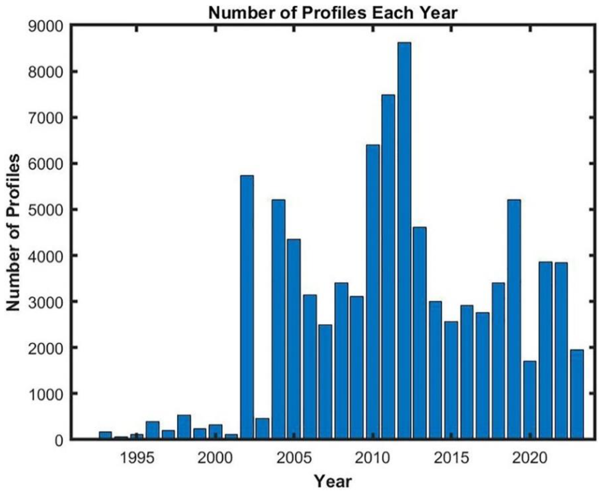
Figure 4. A total of 88,412 profiles, collected from 1993 to 2023, were analyzed from the Millstone Hill Incoherent Scatter Radar to calculate the Peak Density Thickness (PDT), categorized by the four seasons. These visuals depict 2D filled contour plots derived from 2D histograms. Each histogram includes 24 bins for the hours of the day and 10 km bins for various PDT values. The color gradient, spanning from blue to red, shows the number of profiles within each bin, offering a detailed overview of the PDT’s diurnal and seasonal variations. (adapted from Shammat et al., 2024).

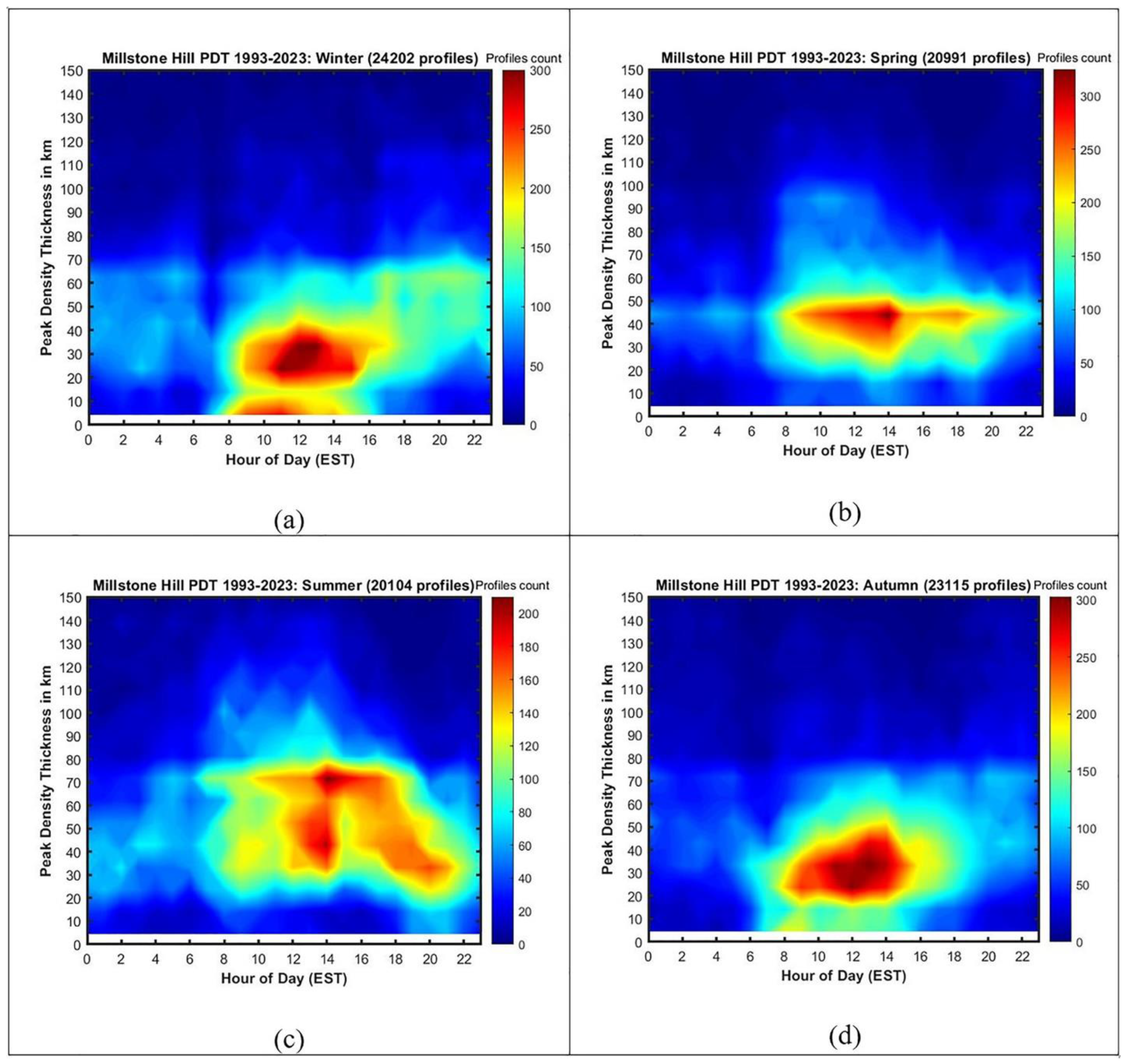
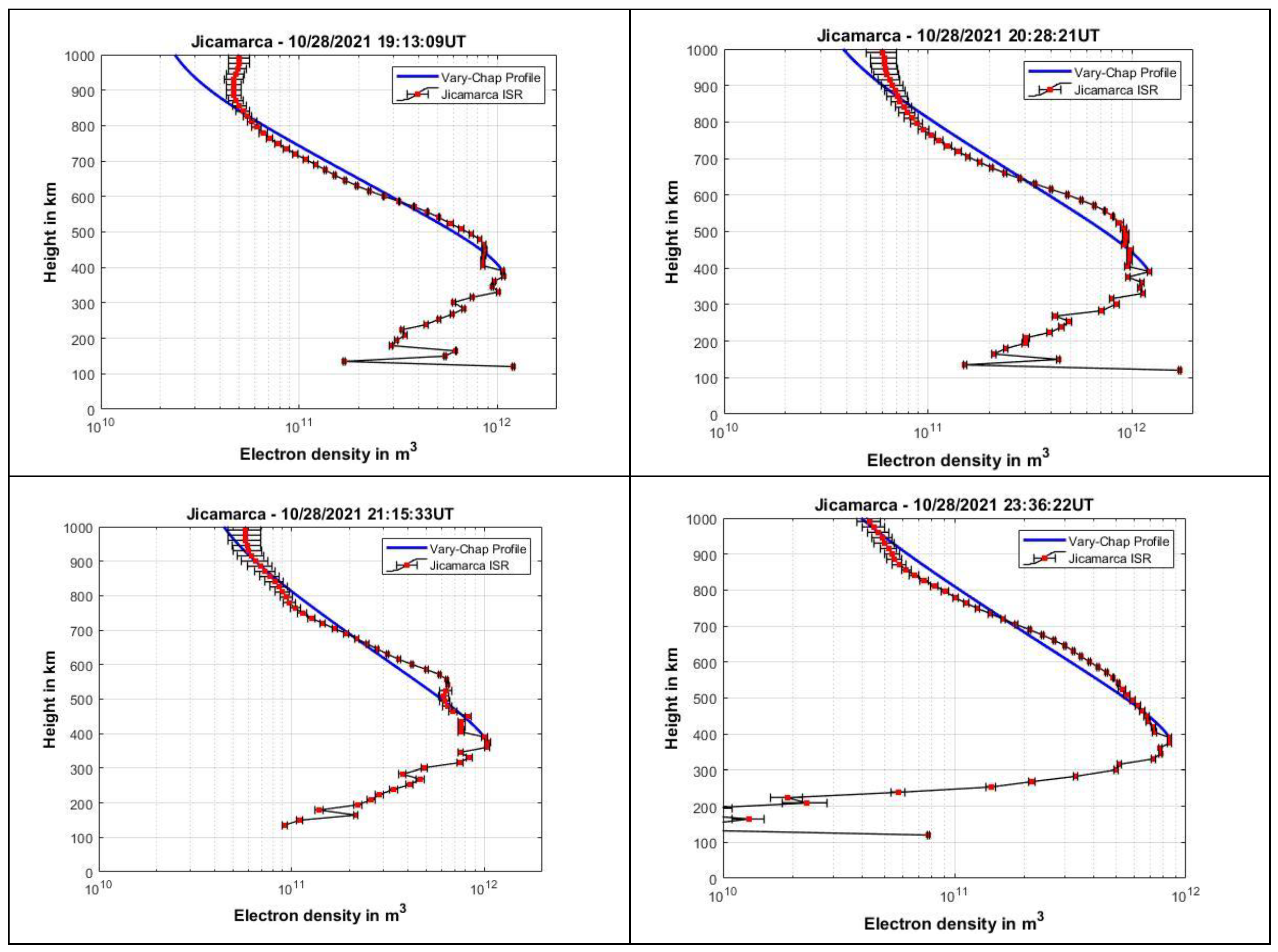
Figure 5. Jicamarca ISR measurements of the full electron density profile on October 28th, 2021, shown in red squares. The Vary-Chap profile is fitted to the topside portion of the ISR measurements and starts from hmF2+PDT as illustrated with the blue line. The figures above represent nighttime and early morning (7:00 pm -7:00 am) local time in Lima. No PDT was observed during this time window.

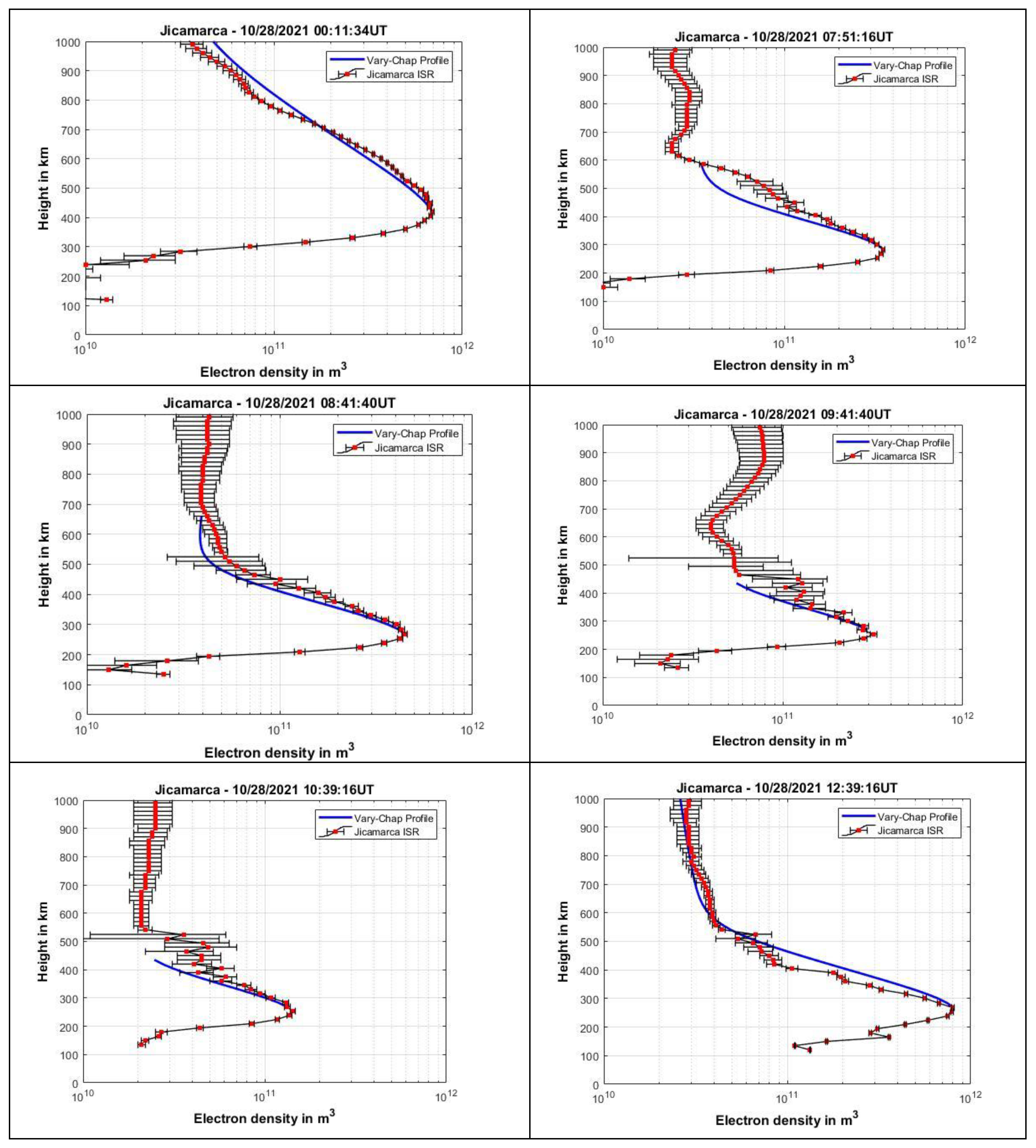
Figure 6. Jicamarca ISR measurements of the full electron density profile on October 28th, 2021, shown in red squares. The Vary-Chap profile is fitted to the topside portion of the ISR measurements and starts from hmF2+PDT as illustrated with the blue line. The figures above represent daytime (8:34 am -1:32 pm) local time in Lima. PDT was observed during this time window ranging from 0 km at 8:34 am local time to 150 km at 1:32 pm local time.

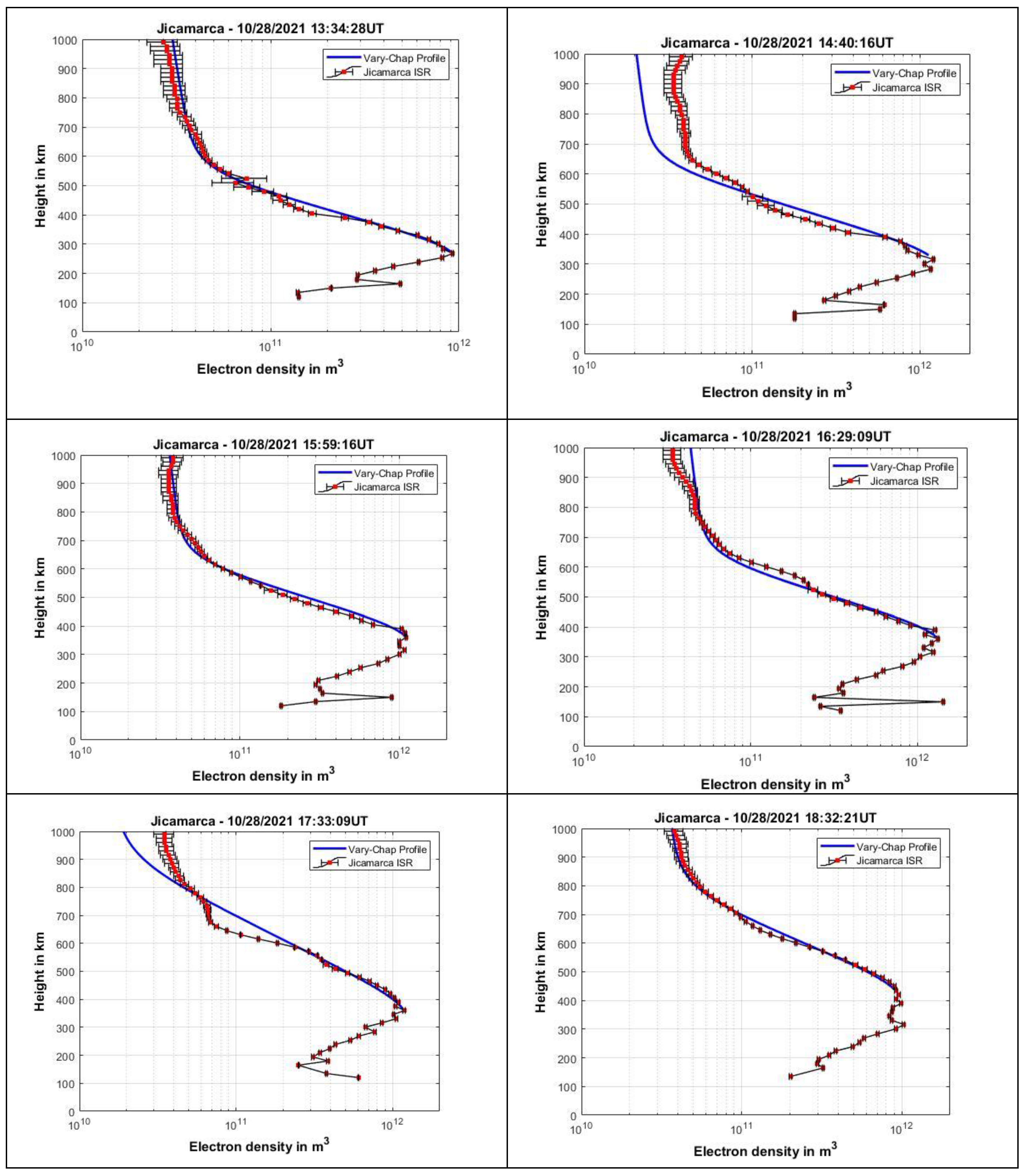
Figure 7. Jicamarca ISR measurements of the full electron density profile on October 28th, 2021, shown in red squares. The Vary-Chap profile is fitted to the topside portion of the ISR measurements and starts from hmF2+PDT as illustrated with the blue line. The figures above represent daytime (02:13 pm -6:36 pm) local time in Lima. PDT starts to decrease during this time window.

Conclusion

The Jicamarca ISR experiment conducted on October 28th, 2021, successfully measured the electron density profile around the F2 peak with high altitude resolution. The results demonstrated the existence of a peak density thickness around the F2 peak, which aligns with previous findings at Millstone Hill. The simultaneous measurements from the Digisonde and Vary-Chap model allowed for accurate comparison of the results. The Jicamarca ISR measurements of the full electron density profile over an 18-hour period retrieved from the Madrigal database confirmed the presence of the Peak Density Thickness (PDT) parameter. The findings showed a predominantly flat F2 peak during a 5-hour window around solar noon, consistent with earlier observations. To reconstruct the topside profile, the Vary-Chap topside model was used, starting from hmF2+PDT. Least square fitting was applied to determine the values of the Vary-Chap parameters α, β, and hT. The reconstructed Vary-Chap topside profile closely matched the measured ISR profiles.

This study emphasizes the importance of the PDT parameter in understanding ionospheric plasma dynamics and improving predictive models of ionospheric behavior. These insights contribute significantly to both theoretical research and practical applications in ionospheric science. Future research should continue to explore the implications of PDT across various latitudes and geomagnetic conditions.

References

Chapman, S. (1931). The absorption and dissociative or ionizing effect of monochromatic radiation in an atmosphere on a rotating Earth. Proceedings of the Physical Society, 43(1), 26–45. [CrossRef]
Croft, T. A., & Hoogansian, H. (1968). Exact ray calculations in a quasi-parabolic ionosphere with no magnetic field. Radio Science, 3(1), 69–74. [CrossRef]
Erickson, P. J. (1998). Observations of light ions in the midlatitude and equatorial topside ionosphere. Cornell University.
Erickson, P. J. (2012). ISR, TEC, and SuperDARN capabilities at subauroral latitudes: RBSP coordinated science. In Proc. RBSP SWG IT. JHUAPL, John Hopkins University. Retrieved from https://rbspgway.jhuapl.edu/sites/default/files/20120820/SWG_IT_Session/Erickson_SWG_IT_Inocoh_Radars_21Aug12.pdf.
Evans, J. V. (1965). Ionospheric backscatter observations at Millstone Hill. Planetary and Space Science, 13(11), 1031–1074. [CrossRef]
Fleming, J. A. (1902). Waves and ripples in water, air, and ether. In Proc. Royal Institution of Great Britain (Vol. 17, p. 223).
Gulyaeva, T. L. (1997). TEC residual slab-thickness between bottomside and topside ionosphere. Acta Geodaetica et Geophysica Hungarica, 32(3–4), 355–363. [CrossRef]
Jackson, J. E. (1969). Comparisons between topside and ground-based soundings. In Proceedings of the IEEE (Vol. 57, No. 6, pp. 976–985). [CrossRef]
Nsumei, P., Reinisch, B. W., Huang, X., & Bilitza, D. (2010). Comparing topside and bottomside-measured characteristics of the F2 layer peak. Advances in Space Research, 46(8), 974–983. [CrossRef]
Nsumei, P., Reinisch, B. W., Huang, X., & Bilitza, D. (2012). New Vary-Chap profile of the topside ionosphere electron density distribution for use with the IRI model and the GIRO real time data. Radio Science, 47(4), RS0L16. [CrossRef]
Reinisch, B. W., Nsumei, P., Huang, X., & Bilitza, D. K. (2007). Modeling the F2 topside and plasmasphere for IRI using IMAGE/RPI, and ISIS data. Advances in Space Research, 39(5), 731–738. [CrossRef]
Rishbeth, H., & Garriott, O. K. (1969). Introduction to ionospheric physics. Academic.
Shammat, M. O., Reinisch, B. W., Galkin, I., Erickson, P. J., Weitzen, J. A., & Rideout, W. C. (2024). Characterizing plasma Peak Density Thickness in the Ionosphere: A single-site multi-instrument study. Radio Science, 59, e2023RS007658. [CrossRef]

Disclaimer/Publisher’s Note: The statements, opinions and data contained in all publications are solely those of the individual author(s) and contributor(s) and not of MDPI and/or the editor(s). MDPI and/or the editor(s) disclaim responsibility for any injury to people or property resulting from any ideas, methods, instructions or products referred to in the content.

© 2024 by the authors. Licensee MDPI, Basel, Switzerland. This article is an open access article distributed under the terms and conditions of the Creative Commons Attribution (CC BY) license (http://creativecommons.org/licenses/by/4.0/).

Copyright: This open access article is published under a Creative Commons CC BY 4.0 license, which permit the free download, distribution, and reuse, provided that the author and preprint are cited in any reuse.