
Submitted:
30 July 2024
Posted:
31 July 2024
You are already at the latest version
Abstract
Agriculture is a vital component of Egypt's economy; therefore, using Digital Elevation Models (DEMs) in agricultural planning in Egypt has significant benefits regarding water management, site appropriateness assessment, flood risk mitigation, and infrastructure construction. It is also essential for planners to make more informed decisions, optimize resource allocation, and support sustainable farming practices. This research paper investigates the accuracy of obtaining DEM data from four free global models (STRM30, ALOS30, COP30, and TanDEM-X90). The global DEM data has been compared to an actual GNSS-RTK DEM data surveyed onsite for two agricultural block areas in Aswan, the southern Government of Egypt. The two blocks are a part of a national project. For Block I and II, the RMSE of the Model STRM30 was 2.92 m and 3.59 m, respectively, indicating a poorer solution. Regarding accuracy, the ALOS30 model ranks third, reporting an RMSE of 2.58 m for block II and 3.30 m for block I. COP30 has an RMSE value of 1.06 m for blocks I and II and.91 m overall. TanDEM-X90 is the most accurate model in this investigation; block I provided an RMSE of 0.90 m with an SD of 0.58 m (SD95% = 0.38 m). After removing the anomalies, the model's stated RMSE for block II was 0.34 m, with an SD value of 0.62 m and 1.03 m. According to the classification using machine learning algorithms, with an accuracy of 84.7% for block I and 85% for block II, TanDEM-X90 is the best solution.
Keywords:
DEM
; GNSS-RTK
; Agricultural
; Machine Learning
; Egypt
1. Introduction
Digital elevation models (DEMs) are crucial inputs for environmental and landscape modeling and spatial analysis. These models provide topographic and terrain characteristics, including slope aspect, slope, channels, and hillslopes. [1], especially for geomorphology studies [2], geology [3], hydrology [4], and Civil Engineering [5]. Modeling to prevent natural disasters is one of its applications (floods [6], soil erosion Studies [7], weather forecasting [8], and climate change [9]). Digital Surface Model (DSM), Digital Terrain Model (DTM), and Digital Elevation Model (DEM) can all sound like they mean different things. The word “DSM” will mean a specific type of DEM, where the elevations cover the buildings, plants, and other things on Earth’s surface. The term “DTM” refers to a model that shows the heights of bare ground. DEM is a broad word that can mean either of these things. It is important to remember that a DEM is a subset of a DTM, even though the names don’t mean the same thing. For this reason, a DTM can show more anatomical details. [10].
To use a Digital Elevation Model (DEM), it is essential to have a coordinate system and a reference frame. The data components include horizontal, vertical, and temporal elements, which must be specified in the metadata. Datums are established at various scales (global, regional, national, or local) and throughout different historical periods. Selecting a horizontal datum, often WGS84 or a similar standard, determines the relationship between latitude and longitude coordinates and the Earth’s surface. The vertical datum establishes the reference point for measuring elevations and can be based on either an ellipsoidal or geoidal (mean sea level) frame of reference. Global geoidal datums, like EGM2008 [11] and EGM96 [12] are possible. Figure 1 shows the relations between ellipsoidal height (h), orthometric height (H), and geoid undulation (N). The ellipsoidal height is estimated using Equation (1) [13].
h=H+N
Various surveying techniques are used to create the digital elevation model (DEM). [14] Compare the DEM created by Total station and those using post-processing kinematic single frequency GPS data. [15] studied the efficiency of the GNSS-PPP solution [16] and [17] in comparison to the GNSS differential solution [17]. The study showed that the Root Mean Square Error (RMSE) was 2-3 cm between the differential and PPP solution. In addition to the classical survey, DEM is established through various methods, including airborne or satellite-borne stereoscopic photogrammetry, interferometry of RADAR or SAR, and airborne laser scanning. Each technique’s limitations depend on cost, precision, sample density, and preprocessing prerequisites. Typically, a DEM-generated procedure comprises four steps: data acquisition, resampling of grid spacing, height interpolation, repetition, and accuracy evaluation [18]. [19] explained that the error of the DEM is associated with grid spacing and interpolating techniques as well as resampling methods. These errors on a DEM spatial scale have been categorized as gross errors resulting from data collection, systematic errors arising from the establishment of elevation height values in the stereo image, and random errors arising from unknown sources. The variability of their defects across different terrains is due to topographical conditions [20]. Nowadays, different open-source Global DEMs are downloadable free of charge from the official provider’s websites, such as the Shuttle Radar Topography Mission (SRTM) [21,22], ALOS Global Digital Surface Model (AW3D30) [23], and TanDEM-X [24].
Many researchers investigated the accuracy of such free DEMs in various disciplines. [25] assessed the effectiveness of AW3D30, TanDEM-X, and SRTM- across four distinct geographical regions characterized by diverse topography and land cover conditions. The study adjusted the resolution of the global models to match a reference model resolution of 1 m. It then assessed the accuracy by creating error rosters and producing descriptive statistics. The study found that slope had the most significant impact on the accuracy of the Digital Elevation Model (DEM), with AW3D30 exhibiting the highest level of durability and stability. In addition, SRTM showed a slight improvement; moreover, TanDEM-X performed the worst in all case studies. [26] This study assesses the precision of Digital Elevation Model (DEM) products across different topography and land cover regions and features. It focuses on a specific case study conducted on Shikoku Island, Japan. Digital Elevation Models (DEMs) are employed in scientific investigations and have been produced by several techniques, including Stereoscopic Photogrammetry, RADAR-SAR interferometry, LIDAR, and GPS. The generated data exhibit errors in the topography and land cover classification. The study assesses six open-source digital elevation models (DEMs) and their characteristics in Shikoku Island, Japan, by comparing them to reference elevation points obtained through GPS observations. The error of digital elevation models (DEMs) has been found to affect the characteristics of the terrain. The accuracy values of high-resolution digital elevation models (DEMs) based on the root mean square error (RMSE) are 9.9 m and 10.1 m for ASTER and SRTM, respectively.[27] conduct an initial evaluation of the accuracy of TanDEM-X for specific floodplain locations and compare it to widely used global digital elevation models (DEMs) of the SRTM model. The results demonstrate that TanDEM-X exhibits comparable average vertical accuracy, which is a substantial enhancement over SRTM. An analysis was conducted to evaluate vertical accuracy based on land cover. The findings indicate that the TanDEM-X model is the most precise global digital elevation model (DEM) across all land cover categories.
[28] examined the accuracy of elevation data obtained from six major publicly available satellite-derived Digital Elevation Models (DEM). The study also investigated the extent to which accuracy can be improved by applying a correction method (linear fit) using Differential Global Positioning System (DGPS) estimates at Ground Control Points (GCPs). The study area consists of a rugged rock terrain that is predominantly flat but also contains undulating and uneven surfaces. Additionally, the study explored the impact of resampling methods and determined the optimal number of ground control points (GCPs) to minimize errors for future applications. Utilizing DGPS data at GCPs significantly reduces bias by eliminating systematic error. Therefore, correcting DEMs with DGPS before utilizing them in scientific research is advisable. [29] studied the topography of 3837 km2 in Lower Tapi Basin, India, the accuracy of SRTM30 and AW3D30 models compared to 117 GCPs. The obtained DEM provided an RMS error of 2.88 m and 2.45 m for the SRTM and AW3D30 models, respectively. For 23,235 km2 in the Egyptian Delta, [30] obtained an RMS error of 2.35 m and 2.19 m from STRM30 and AW3D30 models using 200 GCPs. The accuracy of the original TanDEM-X DEM and its enhanced edited variant, the Copernicus DEM, was assessed in [30] across three prominent mountain ranges in Europe: the Alps, the Carpathians, and the Pyrenees. The evaluation used a standard digital surface model derived from airborne laser scanning data. Furthermore, it assesses the suitability of terrain attributes (slope, aspect, and altitude) and data acquisition characteristics (coverage map, consistency mask, and height error map) for locating problematic sites. They have demonstrated that the Copernicus DEM at 30 m and 90 m resolutions represent the Earth’s surface with greater precision than the TanDEM-X-90 and SRTM DEMs.
Agriculture is essential to Egypt’s economy, providing job opportunities and guaranteeing food security for its rising population. DEMs are particularly important in Egypt’s agriculture, as topography influences water management, soil fertility, and crop compatibility. This motivation statement intends to emphasize the motivations for investigating DEMs and their use in agricultural practices in Egypt. The following points highlight the importance of the DEM model in agriculture.
- Sustainable agriculture in Egypt requires effective water management due to limited water resources. DEMs offer detailed information about topography and terrain features, making it possible to identify and map watersheds, drainage patterns, and potential water storage areas. Researchers and water resource managers can use DEMs to improve irrigation planning, implement precision water application techniques, and develop effective water conservation and allocation strategies.
- Precision farming and crop compatibility: To find out which crops will grow well together and use precision farming methods, it’s important to know how the land’s features and changes affect farming areas. DEMs give elevation information, which can be combined with other geographical details like soil type, sun exposure, and slope to figure out which areas are best for growing certain foods. When farmers learn about DEMs, they can make better decisions about which crops to grow, how to put them, and how much fertilizer to use. This leads to higher yields and better use of resources.
- Effective land use planning aims to facilitate sustainable growth and optimize agricultural capacity. Digital Elevation Models (DEMs) encompass crucial data about the heights of land, the shapes of landforms, and the differences in land cover. Data-driven ecosystem models (DEMs) empower legislators, urban planners, and agricultural authorities to make informed choices about land allocation, zoning regulations, and infrastructure advancement. This data aids Egypt in optimizing the utilization of land resources, attaining harmonious urban-rural development, and fostering agricultural growth.
Applying Digital Elevation Models (DEMs) to agricultural planning in Egypt provides considerable benefits in water management, site suitability evaluation, soil conservation, flood risk mitigation, and infrastructure development. Researchers, farmers, and planners may make more informed decisions by investigating DEMs, optimizing resource allocation, and encouraging sustainable agricultural practices. Integrating DEMs with other geospatial data improves agricultural production, resilience, and long-term development in Egypt’s farming industry.
2. Materials and Methods
2.1. GNSS Solution
Using multiple GNSS constellations for positioning improves accuracy, dilution of precision (DOP), availability, and reliability [31]. Currently, there are four GNSS operating systems: NAVSTAR GPS (American), GLONASS (Russian), Galileo (European), and BeiDou (Chinese). However, until 2019, only GPS and GLONASS have been operational. Relative positioning, sometimes called differential Global Navigation Satellite Systems (DGNSS), is one technique for attaining centimeter-level positional precision. DGNSS uses a fixed, known position ground reference station (base station) to increase positioning accuracy. The rover, the second GNSS receiver, has two modes of operation: kinematic and static. Both receivers need to watch the identical satellites simultaneously. Since the errors affecting the base and rover’s observations are similar, it is possible to estimate the baseline between them [17]. More details about the technique of GNSS can be seen in [13,17,16].
2.2. SRTM3-30 DEM
The National Aeronautics and Space Administration (NASA), the National Geospatial-Intelligence Agency (NGA), the German Space Agency (DLR), and the Italian Space Agency (ASI) collaborated on the Shuttle Radar Topography Mission (SRTM). This international project launched in February 200 [32]. First, a worldwide C-band DEM version with a spatial resolution of 90 m (3 arcsec) was made available by the United States Geological Survey (USGS) in 2003. This version was the first near-global high-resolution DEM created [33]. Subsequently, SRTM2 (version 2) was developed, including multiple enhancements in terms of eliminating artifacts (such as pits and spikes) and taking into account water bodies and coasts [34]. NASA made the third version of SRTM3 (“SRTM Plus”) free in September 2014. It has a spatial resolution of 30 m. This version was much better than the low-resolution SRTM1 (90 m), which only covered areas outside the US [35]. The dataset might be downloaded from [https://lta.cr.usgs.gov/].
2.3. AW3D-30 DEM
The Japan Aerospace Exploration Agency (JAXA) launched the Panchromatic Remote Sensing Instrument for Stereo Mapping (PRISM) sensor in January 2006 on the ALOS (Advanced Land Observing Satellite) satellite. About 3 million of the 6.5 million pictures that ALOS produced during the mission (from roughly 80° N latitude to 80° S latitude) had cloud cover of less than 30%, which was used to create a global 5-m (0.15 arcsec) image. [36]. A 30-m resolution version (AW3D30), which is a resampling of the 5-m version, was made publicly available in 2016 [37]. The dataset might be downloaded from [https://www.eorc.jaxa.jp/ALOS/en/index_e.htm].
2.4. TanDEM-X-90 DEM
TanDEM-X (TerraSAR-X add-on for digital elevation measurement) is a high-resolution interferometric SAR (InSAR) radar introduced by the German government in 2010 Aerospace Center (DLR), in collaboration with EADS Astrium GmbH and Infoterra GmbH (public-private partnership) consortium [38]. TanDEM-X radar collects Earth data in tandem with TerraSAR-X (launched in June 2007) as a single satellite spacecraft (TerraSARX/ TanDEM-X) in a controlled orbit with a baseline of 250-500 m [37]. The dataset might be downloaded from [http://tandemx-science.dlr.de/].
2.5. Copernicus-30 DEM
The Copernicus DEM is a Digital Surface Model (DSM) that accurately depicts the Earth’s surface, encompassing structures, infrastructure, and vegetation. This DSM is a modified version of WorldDEM, with added features such as smoothing water bodies and representing rivers with regular flow. Furthermore, modifications have been made to shorelines and coastlines and specific elements like airports and unrealistic terrain formations. The WorldDEM product is built on radar satellite data collected during the TanDEM-X Mission. This mission is paid for by a public-private partnership between the German government through the German Aerospace Centre (DLR) and Airbus Defence and Space. The global 30m (GLO-30) and 90m (GLO-90) are available through OpenTopography [39].
The following table concludes some characteristics of the four DEM models.

Table 1.
DEM Characteristics.
| DEM | Resolution | Vertical Reference | Description |
|---|---|---|---|
| SRTM3-30 | 30 m | EGM96 | https://lta.cr.usgs.gov/. |
| AW3D-30 | 30 m | EGM96 | https://www.eorc.jaxa.jp/ALOS/en/index_e.htm |
| TanDEM-X-90 | 90 m | WGS84 | http://tandemx-science.dlr.de/ |
| Copernicus-30 | 30 m | EGM2008 | OpenTopography - Copernicus GLO-30 Digital Elevation Model |
2.6. GIS Solution
Geographic Information Systems (GIS) were initially mentioned in published literature in the mid-1960s. A geographic information system combines hardware, software, data, and organizational structure to gather, store, manipulate, and analyze “geo-referenced” data and present the results. A Geographic Information System (GIS) collects, stores, and retrieves information based on spatial location. It also identifies specific areas within a target environment. It investigates the relationships between data sets within an environment. It also analyses spatially to aid decision-making and selects and passes data to application-specific analytical models to assess the impact of alternatives on the chosen environment. Finally, GIS displays the selected environment graphically and numerically before and after analysis [40]. Most of the research has used GIS tools to extract the DEM data from the satellite images provided by different sources, as mentioned in [41,42,43].
3. Methodology
The experimental studies are in Kom Ombo- Aswan government- Egypt as part of the Future of Egypt for Sustainability national project. This project aims to reclaim around 850,000 acres on Aswan’s west bank of the River Nile. Two blocks were surveyed using the GNSS-RTK method to obtain the different levels inside, which helps the designers detect the possible levels for the irrigation pivot systems. The first block has 5090 Acres, and the second has 6985 Acres. Figure 2 shows the map of the two case studies.
3.1. GNSS-RTK Solution
A reliable Real-Time Kinematic (RTK) solution requires a static GPS solution. RTK is a technique for improving GPS positioning accuracy by utilizing data from a fixed reference station, commonly called a base station. A static GNSS station list was constructed on each block for this purpose. The stations have been observed using Trimble GNSS receivers depending on reference control points belonging to the General Authority for Roads and Bridges (GARB) [https://garb.gov.eg/]. These control points were referenced with the global coordinates system of (WGS84/UTM zone 36N) and based on EGM2008 as a geoid model. Figure 3a refers to the Trimble R4S GNSS receiver as a known base station, while Figure 3b refers to the rover with the Trimble R2 GNSS receiver. In addition, Figure 3c shows the 4*4 pickup car used to get the GNSS RTK kinematic DEM data using the Trimble R2 GNSS receiver. The rover was fixed over the vehicle; the moving paths were divided over the area and inserted into the controller—five static C.Ps. Five C.P.s have been observed on-site for Block I and 13 stations for Block II, which were corrected based on a main C.P. Trimble Business Centre V. 5.2 (TBC v.5.2), which was used to process the static Rinex observations data.
The vertical accuracy of any DEM is defined as the discrepancies (d), which refers to the accuracy in the height obtained by the reference height (hRTK) solution and the height derived from the other four DEMs (hDEM) in the study. The discrepancies are expressed as to be seen in Equation (2). According to Equations, the standard deviation (SD), which refers to the deviation relative to the mean value (µ), is estimated in the study. ((3)-(4)). Then, an SD of 95% is estimated by filtering the random errors. To calculate the absolute accuracy of each DEM model, the Root mean square error (RMSE) is estimated according to Equation (5).
di=hDEM, i - hRTK,i
Figure 4Error! Reference source not found. Explains the flowchart of the analysis procedure; this flowchart provides five analysis stages. The first stage is the static solution. Stage (2) refers to the RTK solution; this solution is referenced with different geoid models (WGS84- EMG96- EGM2008) according to the reference height for each DEM model. Stage (3) denotes the DEM global solution and the related height reference. Stage (4) estimates errors according to equation (1). The final step (stage (5)) refers to the statistics estimation (min, mean, max., SD, and RMSE) according to Equations ((2)–(5)).
4. Results and Discussions
The absolute vertical errors were estimated between the reference height delivered from the GNSS-RTK solution and the global DEM solution obtained from the four examined models for block 1. The distribution of vertical error by DEM is plotted in Figure 5, and the descriptive statistics can be found in Table 2.
Table 2 shows the absolute vertical accuracy of STRM 30, ALOS 30, COP 30, and TanDEMX90 models for block 1; the total number of points is (34854) randomly points on-site.
- Model STRM30 exhibits a mean error range of -1.62 meters, encompassing the outliers (-33.16 to 21.27 m). This model shows an RMSE of 3.59 meters and an SD of 3.20 meters; the SD95% is 2.26 meters after anomalies are eliminated.
- Model ALOS30 shows an error range of (-21.97-15.19 m) with a mean value of -2.8 m and a Root Mean Square Error (RMSE) of 3.30 m. After removing the outliers, the solution initially had a standard deviation of 1.75 m, which decreased to 0.99 m.
- The COP30 model has an error range of -10.83 to -5.42 m, with a mean value of -0.65 m. Moreover, the solution shows a Root Mean Square Error (RMSE) of 0.91 m and a Standard Deviation (SD) of 0.64 m (95% Confidence Interval for SD = 0.43 m).
- The TanDEMX90 model offers the optimal solution, with an error range of -4.22 to 5.11 meters and a mean value of -0.69 meters. The result displayed here has a Root Mean Square Error (RMSE) of 0.90 and a Standard Deviation (SD) of 0.58 meters, with a 95% confidence interval of 0.38 meters.
Table 2 reveals that both the COP30 model and TanDEX90 model are more accurate than Model STRM30 and Model ALOS30. Model STRM30 and Model ALOS30 have more errors and deviations in the negative direction, where the mean values are (-1.62 m) for model STRM30 and (-2.8 m) for model ALOS30. At the same time, these metrics are greater than those reported by the COP30 model and TanDEX90 model. It should be noted that the COP30 model used a 30 m resolution of pixels for their analysis, while the TanDEX90 model used a 90 m resolution of pixels. The TanDEX90 model has marginally higher accuracy than the COP30 model; it was better. TanDEX90 model has slightly RMSE (0.90 m) and SD (0.58 m) before correlation. In addition, the TanDEX90 model has a relatively more significant R-value (0.9977) than the COP30 model before correlation.
Figure 5 reveals the vertical errors in DEM-STRM and DEM-ALOS 30 have a more normal shape, being unimodal and symmetric. In contrast, DEM-COP 30 and DEM-TanDEMX 90 errors have a strikingly biomo1dal distribution. The jug nature of the SRTM distribution is likely due to elevation values being given as integers. The density distribution of errors in Figure 5 shows a red color line (reference (zero) line) and a wider spread of errors for DEM-STRM and DEM-ALOS 30 compared to COP30 model and TanDEX90 model, where the error distribution was around (6-8) m in the case of DEM-STRM as shown in Figure 5, while the errors decreased gradually (2-4) m for DEM-ALOS 30. This is also evidenced by the Min, Mean, and Max values (for example, the Mean value for the TanDEX90 model was (-0.69) compared to (-1.62) for DEM-STRM). Considering the density distribution of errors and the descriptive statistics computed in Table 2, The TanDEMX90 model is the most accurate compared to all models for block I. The TanDEMX90 model has more verticality and homogenous data, less error, and a more acceptable data shape. Correlation between levels using RTK and Z or Height for all four models was computed as shown in Figure 6 below.
RMSE is a quadratic metric that puts greater weight on large error values; thus, although the errors in TanDEMX90 are more minor, the more significant errors are distorting the RMSE score despite the use of removing outliers. R95% and SD95% (m) were computed using a 5% error assumption to convert the data shape to the standard Gaussian distribution. The results were 43 cm (SD95% for TanDEMX90) and 38 cm for COP 30. Figure 6 shows the correlation of the relationship shape between the same verticality points for the four models with RTK solution. The X-axis represents levels of points using the RTK solution, and the Y-axis represents the Height for the same point (Z or H). The Y-axis ranges from 130 to 200. If the data were homogenous and had a high degree of similarity, the correlation would be approximately 1.0; otherwise, the correlation would be less than 1.0. The upper four graphs of Figure 6 show the results of correlation without filtering, whereas the lower four graphs of Figure 6 show the results of correlation after 5% filtering. The results from correlation show that R95% for TanDEMX90 equals (0.9999), and this value is four models, So TanDEMX90 from German space is the best.
The same procedure and the estimation of the absolute vertical errors between the reference height solution delivered from the GNSS-RTK solution and the global DEM solution obtained from the four models was done for block II, as shown in Table 3, Figure 7 and Figure 8, respectively. Table 3 shows the total No. Of points is (49471) randomly points on-site for Block II, the descriptive statistics display that TanDEMX90 is the most accurate of all (RMSE (1.03 m), SD (0.62 m), Mean (-0.82 m), Min (-7.84 m), Max (3.87 m)).
Figure 7 and Figure 8, respectively, show the density distribution of errors for Block II and the correlation between absolute vertical errors between the reference height solution delivered from the GNSS-RTK and the global DEM for the four models. The results for Block II are harmonious with those for Block I, where TanDEX90 was the most accurate for Block II and R95% for Block II (0.9993 m). This means that TanDEX90 has more verticality and homogenous data and less error for both Block I and II.
5. Machine Learning Analysis
Recently, many efforts have been made to improve the quality and quantity of detected and identified coordinate points on specific blocks on Earth depending on satellite systems. These extracted and obtained data from different DEM solutions need validation by comparing and matching them to the extracted images from GPS regarding coordination systems, boundaries, and essential points on the specific blocks on Earth [44]. As many methods were proposed and performed, such as DEM solutions in this field, machine learning came to validate these methods and identify the most accurate solutions to be considered and recommended in future directions of the survey field studies [45]. In this research, the Support Vector Machine Model (SVM) was used to measure the ability of the selected DEM solutions to detect the exact coordination system of the extracted images from the satellite system using GNSS-RTK for the two different blocks in Egypt. SVM is a binary detection model that uses two categories of high-dimensional data sets to predict the performance of the input parameters. It is initially used to solve and work with classification problems with binary aspects (0,1) [46].
The performance of the previously mentioned methods was analyzed using a machine learning model named Support Vector Machine, and the performance of each selected method was studied and tested separately according to the model in a binary comparison. The GNSS-RTK data was obtained from a GNSS system and considered significant, actual values to be used for measuring the validation of other methods in conducting the satellite data. Therefore, the research focused on measuring each selected method’s efficiency and ability to determine the boundaries and choose regular points of two-block samples of land plots in inaccurate ways.
Four DEM solutions were considered in the selected machine learning model, including STRM-EGM96, ALOS-EGM96, COP30-EGM2008, and TanDEMX90-WGS84. The proper reference DEM solution was chosen, which is GNSS-RTK. The dataset was divided into testing and training sets at 30:70 for each SVM model development. Different sample sizes were trained using the selected machine learning model to be used later for testing the rest of the obtained data, with about 10,400 readings from sample 1 and about 10,000 from sample 2, as seen in Table 4 and Table 5, respectively. The Tables show the efficiency of the four DEM solutions in detecting the correct points on the selected blocks.
Table 4 shows the efficiency of using the selected four DEM solutions in identifying and determining the proper and correct (x, y, and z) values from Block I. The results are relatively close to each other. More clearly, the results show that the accuracy of detecting the points on Block I using the DEM-TanDEMX90-WGS84 was significant and achieved higher accuracy values than the other selected DEM solutions, with about 84.7%. Also, the results reveal that the recall values are relatively low, and the different metrics, like precision and f1-score values, show relatively high values.
In addition, the COP30-EGM2008 solution results show a high accuracy value of about 83.8%. The accuracy results of the STRM-EGM96 and ALOS-EGM96 are relatively low compared to the TanDEMX90-WGS84 results, with about 83.8% and 83%, respectively. Moreover, the metric values of the model, including precision, recall, and f1-score, show the ability of the selected DEM solution to detect and identify the correct points that match the GNSS-RTK solution values for Block I.
In Table 5, the results show that the selected DEM solution, called TanDEMX90 WGS84, is significant in detecting and identifying the points on Block II that match data obtained from the GNSS-RTK solution, with an accuracy of about 85.3%. In contrast, the lower accuracy value at about 83% is achieved by using the STRM-EGM96. Also, the other DEM solutions show acceptable and high accuracy values, with about 85% for the COP30-EGM2008 and 83.1% for the ALOS-EGM96. This relatively low accuracy variance between the two previously selected DEM solutions reveals the significance of these methods for further studies that aim to detect and determine the valid points of blocks on Earth.
6. Conclusions
With the huge developments in agriculture in the Egypt sector, this paper evaluates the free DEM models’ accuracy compared to the GNSS-RTK solution. Four DEM models have been evlauted [STRM30, ALOS30, COP30, and TanDEM-X90]. The experimental research is being conducted in Kom Ombo, Aswan, Egypt, as part of the National Future of Egypt for Sustainability project. This project intends to reclaim around 850,000 acres along Aswan’s west bank of the Nile. Two blocks were surveyed using the GNSS-RTK approach to determine the various levels inside, allowing the designers to identify potential levels for irrigation pivot systems. The first block has 5090 acres, while the second has 6985 acres.
The following are the conclusions of the research paper:
- The reference data for the evaluation is a GNSS-RTK solution with Static-GNSS control points to strengthen the reliability of the results.
- Model STRM30 delivered the worst solution with an RMSE of 3.59 m and 2.92 m for Block I and II, respectively.
- The ALOS30 model comes third according to accuracy, which reported an RMSE of 3.30 m for block I and 2.58 m for block II.
- Model COP30 is the second one with an RMSE value of .91 m and a value of 1.06 m for blocks I and II.
- The best accurate model from this study is TanDEM-X90, which offered an RMSE of 0.90 m for block I with an SD of 0.58 m (SD95% = 0.38 m). Regarding block II, the model reported an RMSE of 1.03 m with an SD value of 0.62 m, and after eliminating the anomalies, was 0.34 m. This result is very optimistic, suggesting that the high resolution from this model might improve the DEM results significantly compared to the truth values using the GNSS-RTK solution.
- By using the machine learning techniques, the classification showed that as well as the classical comparison, TanDEM-X90 is the best solution with an accuracy of 84.7% for block I and 85% for block II.
References
- Rahmati, O.; Yousefi, S.; Kalantari, Z.; Uuemaa, E.; Teimurian, T.; Keesstra, S.; Pham, T.D.; Tien Bui, D. Multi-hazard exposure mapping using machine learning techniques: A case study from Iran. Remote Sensing 2019, 11, 1943. [Google Scholar] [CrossRef]
- Scown, M.W.; Thoms, M.C.; De Jager, N.R. Floodplain complexity and surface metrics: Influences of scale and geomorphology. Geomorphology 2015, 245, 102–116. [Google Scholar] [CrossRef]
- Bonilla-Sierra, V.; Scholtes, L.; Donzé, F.V.; Elmouttie, M.K. Rock slope stability analysis using photogrammetric data and DFN–DEM modeling. Acta Geotechnica 2015, 10, 497–511. [Google Scholar] [CrossRef]
- Fenta, A.A.; Kifle, A.; Gebreyohannes, T.; Hailu, G. Spatial analysis of groundwater potential using remote sensing and GIS-based multi-criteria evaluation in Raya Valley, northern Ethiopia. Hydrogeology Journal 2015, 23, 195. [Google Scholar] [CrossRef]
- He, Y.; Song, Z.; Liu, Z. Updating highway asset inventory using airborne LiDAR. Measurement 2017, 104, 132–141. [Google Scholar] [CrossRef]
- Zhang, K.; Gann, D.; Ross, M.; Robertson, Q.; Sarmiento, J.; Santana, S.; Rhome, J.; Fritz, C. Accuracy assessment of ASTER, SRTM, ALOS, and TDX DEMs for Hispaniola and implications for mapping vulnerability to coastal flooding. Remote sensing of Environment 2019, 225, 290–306. [Google Scholar] [CrossRef]
- Li, L.; Nearing, M.A.; Nichols, M.H.; Polyakov, V.O.; Guertin, D.P.; Cavanaugh, M.L. The effects of DEM interpolation on quantifying soil surface roughness using terrestrial LiDAR. Soil and Tillage Research 2020, 198, 104520. [Google Scholar] [CrossRef]
- Heo, J.; Jung, J.; Kim, B.; Han, S. Digital elevation model-based convolutional neural network modeling for searching of high solar energy regions. Applied energy 2020, 262, 114588. [Google Scholar] [CrossRef]
- Bhatta, B.; Shrestha, S.; Shrestha, P.K.; Talchabhadel, R. Evaluation and application of a SWAT model to assess the climate change impact on the hydrology of the Himalayan River Basin. Catena 2019, 181, 104082. [Google Scholar] [CrossRef]
- Maune, D.F.; S. Kopp, C. Zerdas. Digital elevation model technologies and applications. The DEM Users Manual, 2007.
- Pavlis, N.K.; Holmes, S.A.; Kenyon, S.C.; Factor, J.K. The development and evaluation of the Earth Gravitational Model 2008 (EGM2008). Journal of geophysical research: solid earth 2012, 117(B4). [Google Scholar] [CrossRef]
- Milbert, D.G. and Smith, D.A. November. Converting GPS height into NAVD88 elevation with the GEOID96 geoid height model. In GIS LIS-INTERNATIONAL CONFERENCE, 1996, 1, 681–692. [Google Scholar]
- Leick, A.; L. Rapoport, D. Tatarnikov. GPS satellite surveying. John Wiley & Sons, 2015.
- Farah, A.; A. Talaat, F. Farrag. Accuracy assessment of digital elevation models using GPS. Artificial Satellites 2008, 43, 151–161. [Google Scholar] [CrossRef]
- Abdallah A, Saifeldin A, Abomariam A, Ali R. Efficiency of using GNSS-PPP for digital elevation model (DEM) production. Artificial Satellites 2020, 55, 17–28. [Google Scholar] [CrossRef]
- Abdallah, A. Precise Point Positioning for Kinematic Applications to Improve Hydrographic Survey. Ph.D. Dissertation, University of Stuttgart, Stuttgart, Germany, 2016. [Google Scholar]
- Hofmann-Wellenhof, B.; H. Lichtenegger, E. Wasle. GNSS–global navigation satellite systems: GPS, GLONASS, Galileo, and more. Springer Science & Business Media, 2007.
- Li, J.; Chapman, M.A.; Sun, X. Validation of Satellite-Derived Digital Elevation Models from In-Track IKONOS Stereo Imagery. Ontario Ministry of Transportation: Toronto, ON, Canada, 2006.
- Fisher, P.F.; Tate, N.J. Causes and consequences of error in digital elevation models. Progress in physical Geography 2006, 30, 467–489. [Google Scholar] [CrossRef]
- Hebeler, F. R.S. Purves. The influence of elevation uncertainty on derivation of topographic indices. Geomorphology 2009, 111, 4–16. [Google Scholar] [CrossRef]
- Van Zyl, J.J. The Shuttle Radar Topography Mission (SRTM): a breakthrough in remote sensing of topography. Acta astronautica 2001, 48, 559–565. [Google Scholar] [CrossRef]
- Werner, M. Shuttle radar topography mission (SRTM) mission overview. Frequenz 2001, 55, 75–79. [Google Scholar] [CrossRef]
- Takaku, J.; Tadono, T.; Doutsu, M.; Ohgushi, F. Kai, H. Updates of ‘AW3D30’ALOS global digital surface model with other open access datasets. The International Archives of the Photogrammetry, Remote Sensing and Spatial Information Sciences 2020, 43, 183–189. [Google Scholar] [CrossRef]
- Rizzoli, P.; Martone, M.; Gonzalez, C.; Wecklich, C.; Tridon, D.B.; Bräutigam, B.; Bachmann, M.; Schulze, D.; Fritz, T.; Huber, M. Wessel, B. Generation and performance assessment of the global TanDEM-X digital elevation model. ISPRS Journal of Photogrammetry and Remote Sensing 2020, 132, 119–139. [Google Scholar] [CrossRef]
- Uuemaa, E.; Ahi, S.; Montibeller, B.; Muru, M. and Kmoch, A. Vertical accuracy of freely available global digital elevation models (ASTER, AW3D30, MERIT, TanDEM-X, SRTM, and NASADEM). Remote Sensing 2020, 12, 3482. [Google Scholar] [CrossRef]
- Pakoksung, K. and Takagi, M. Assessment and comparison of Digital Elevation Model (DEM) products in varying topographic, land cover regions and its attribute: a case study in Shikoku Island Japan. Modeling Earth Systems and Environment 2021, 7, 465–484. [Google Scholar] [CrossRef]
- Hawker, L.; Neal, J. and Bates, P. Accuracy assessment of the TanDEM-X 90 Digital Elevation Model for selected floodplain sites. Remote Sensing of Environment 2019, 232, 111319. [Google Scholar] [CrossRef]
- Preety, K.; Prasad, A.K.; Varma, A.K. and El-Askary, H. Accuracy assessment, comparative performance, and enhancement of public domain digital elevation models (ASTER 30 m, SRTM 30 m, CARTOSAT 30 m, SRTM 90 m, MERIT 90 m, and TanDEM-X 90 m) using DGPS. Remote Sensing 2022, 14, 1334. [Google Scholar] [CrossRef]
- Jain, A.O.; Thaker, T.; Chaurasia, A.; Patel, P. Singh, A.K. Vertical accuracy evaluation of SRTM-GL1, GDEM-V2, AW3D30 and CartoDEM-V3. 1 of 30-m resolution with dual frequency GNSS for lower Tapi Basin India. Geocarto International 2018, 33, 1237–1256. [Google Scholar] [CrossRef]
- Marešová, J.; Gdulová, K.; Pracná, P.; Moravec, D.; Gábor, L.; Prošek, J.; Barták, V. Moudrý, V. Applicability of data acquisition characteristics to the identification of local artefacts in global digital elevation models: comparison of the Copernicus and TanDEM-X DEMs. Remote Sensing 2021, 13, 3931. [Google Scholar] [CrossRef]
- Cai, C. Gao, Y. Modeling and assessment of combined GPS/GLONASS precise point positioning. GPS solutions 2013, 17, 223–236. [Google Scholar] [CrossRef]
- Szypuła, B. Quality assessment of DEM derived from topographic maps for geomorphometric purposes. Open Geosciences 2019, 11, 843–865. [Google Scholar] [CrossRef]
- Mashimbye, Z.E.; de Clercq, W.P. Van Niekerk, A. An evaluation of digital elevation models (DEMs) for delineating land components. Geoderma 2014, 213, 312–319. [Google Scholar] [CrossRef]
- DAAC, L. The shuttle radar topography mission (SRTM) collection user guide. Sioux Falls, SD, USA: NASA EOSDIS Land Processes DAAC, USGS Earth Resources Observation and Science (EROS) Center, 2015.
- Rabah, M.; El-Hattab, A. Abdallah, M. Assessment of the most recent satellite based digital elevation models of Egypt. NRIAG journal of astronomy and geophysics 2017, 6, 326–335. [Google Scholar] [CrossRef]
- ALOSWorld3D. Available online: https://portal.opentopography.org/raster?opentopoID=OTALOS.112016.4326.2. (Accessed on 23 December 2023).
- Grohmann, C.H. Evaluation of TanDEM-X DEMs on selected Brazilian sites: Comparison with SRTM, ASTER GDEM and ALOS AW3D30. Remote Sensing of Environment 2018, 212, 121–133. [Google Scholar] [CrossRef]
- DLR-TanDEM-X. Available from: https://www.dlr.de/hr/en/desktopdefault.aspx/tabid-2317/3669_read-5488/. Accessed on 22 December 2023).
- Copernicus, Copernicus Global Digital Elevation Models. Available from: https://portal.opentopography.org/datasetMetadata?otCollectionID=OT.032021.4326.1. (Accessed on 22 December 2023).
- Ghilani, Charles D.; Paul R. Wolf. Elementary surveying. Prentice hall, 2010.
- Wani, Z.M.; Nagai, M. An approach for the precise DEM generation in urban environments using multi-GNSS. Measurement, 2021, 177, 109311. [Google Scholar] [CrossRef]
- Dou, J.; Yunus, A.P.; Tien Bui, D.; Sahana, M.; Chen, C.W.; Zhu, Z.; Wang, W.; Pham, B.T. Evaluating GIS-based multiple statistical models and data mining for earthquake and rainfall-induced landslide susceptibility using the LiDAR DEM. Remote Sensing, 2019, 11, 638. [Google Scholar]
- Nguyen, K.A. and Chen, W. DEM-and GIS-based analysis of soil erosion depth using machine learning. ISPRS International Journal of Geo-Information 2021, 10, 452. [Google Scholar] [CrossRef]
- Habib, A.; Akdim, N.; El Ghandour, F.E.; Labbassi, K.; Khoshelham, K.; Menenti, M. Extraction and accuracy assessment of high-resolution DEM and derived orthoimages from ALOS-PRISM data over Sahel-Doukkala (Morocco). Earth Science Informatics 2017, 10, 197–217. [Google Scholar] [CrossRef]
- Biswal, S.; Sahoo, B.; Jha, M.K.; Bhuyan, M.K. A hybrid machine learning-based multi-DEM ensemble model of river cross-section extraction: Implications on streamflow routing. Journal of Hydrology, 2023, 625, 129951. [Google Scholar] [CrossRef]
- Ziari, H.; Maghrebi, M.; Ayoubinejad, J. and Waller, S.T. Prediction of pavement performance: Application of support vector regression with different kernels. Transportation Research Record 2016, 2589, 135–145. [Google Scholar] [CrossRef]
Figure 1.
Orthometric versus ellipsoidal heights [13].
Figure 1.
Orthometric versus ellipsoidal heights [13].
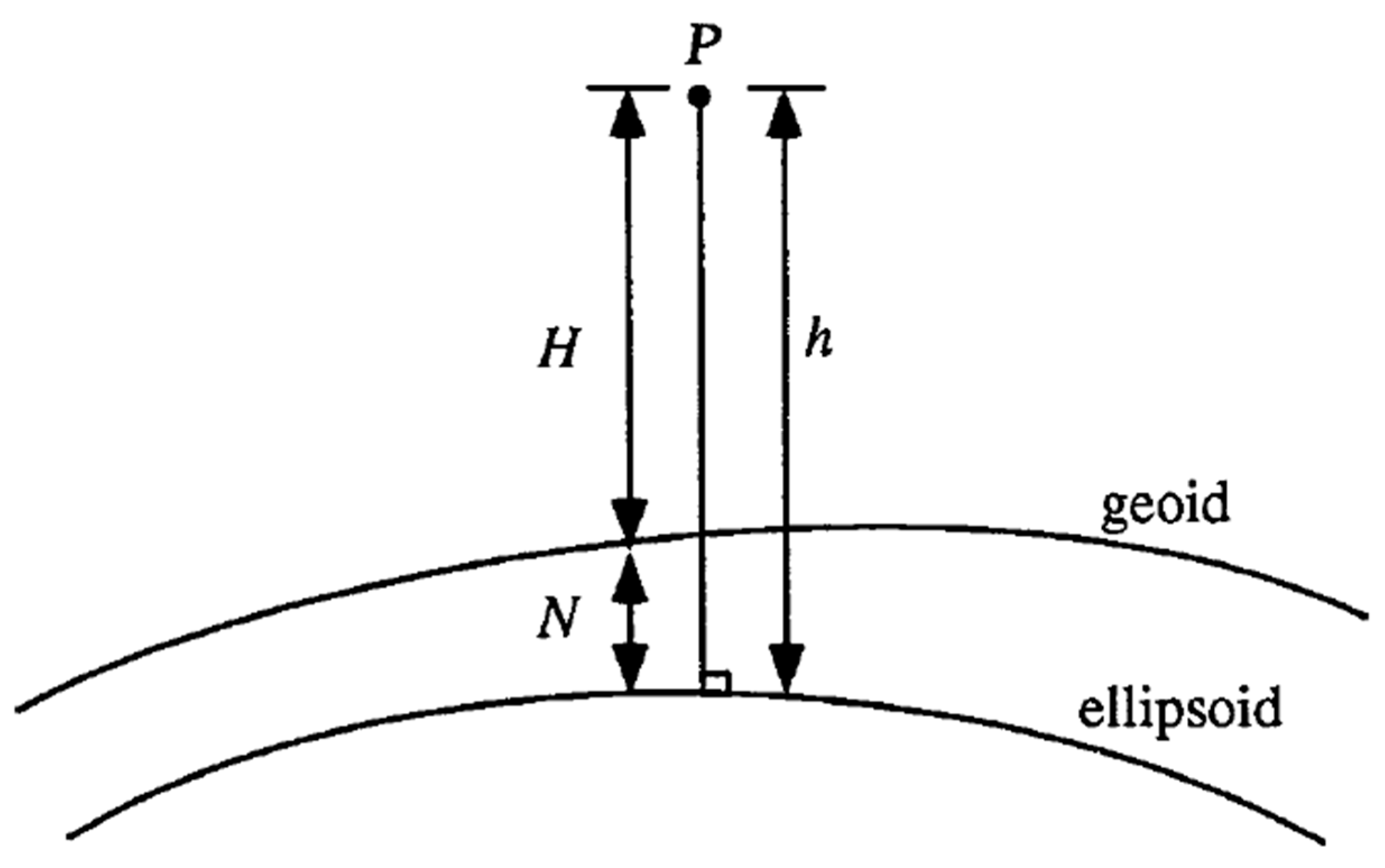
Figure 2.
Map of the two case studies, Block I and II.
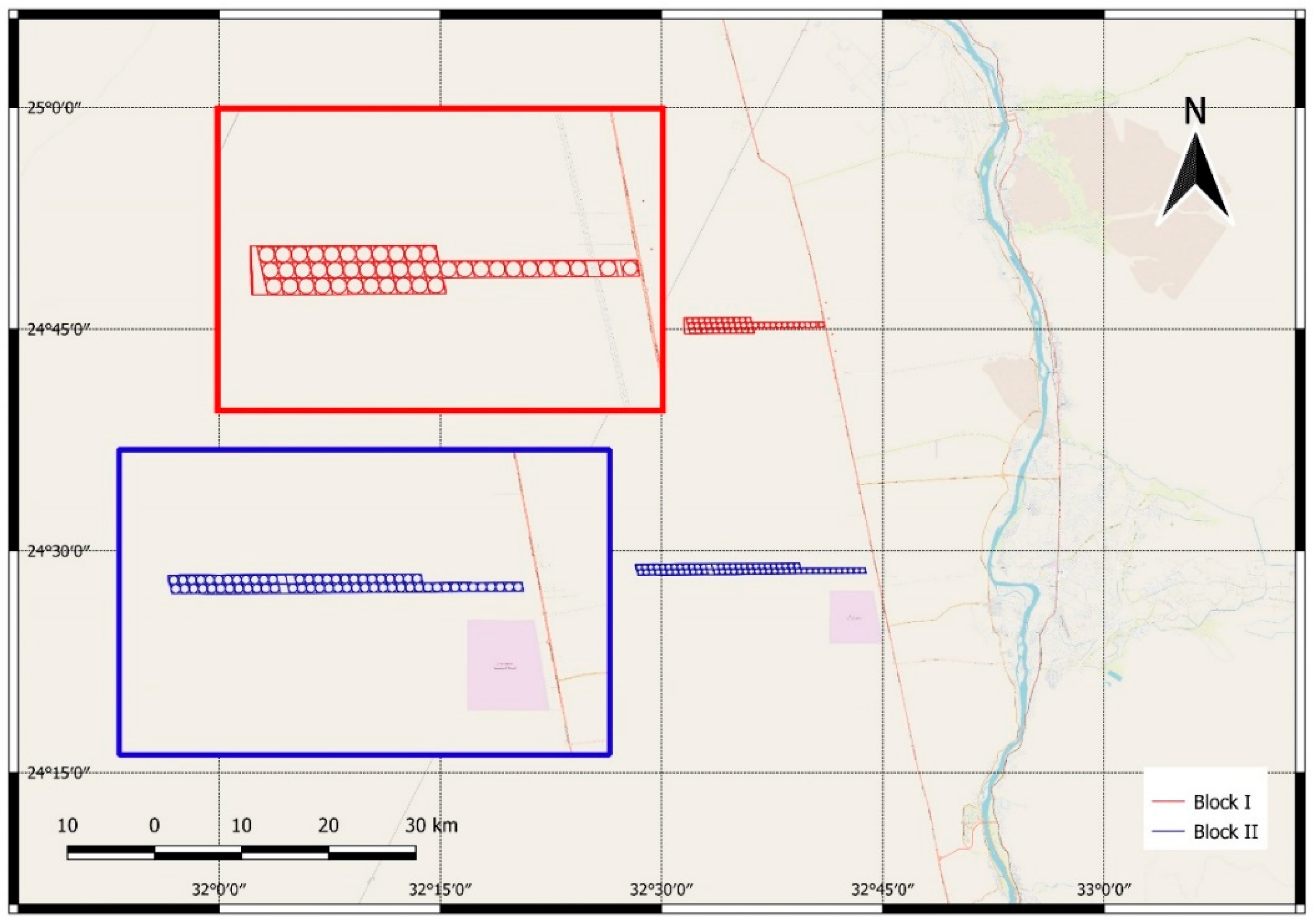
Figure 3.
GNSS receivers over the control points; (a) refers to the base station with Trimble R4S GNSS receiver; (b) refers to the rover station with Trimble R2 GNSS receiver; (c) refers to the GNSS-RTK solution using 4*4 Pickup car.
Figure 3.
GNSS receivers over the control points; (a) refers to the base station with Trimble R4S GNSS receiver; (b) refers to the rover station with Trimble R2 GNSS receiver; (c) refers to the GNSS-RTK solution using 4*4 Pickup car.
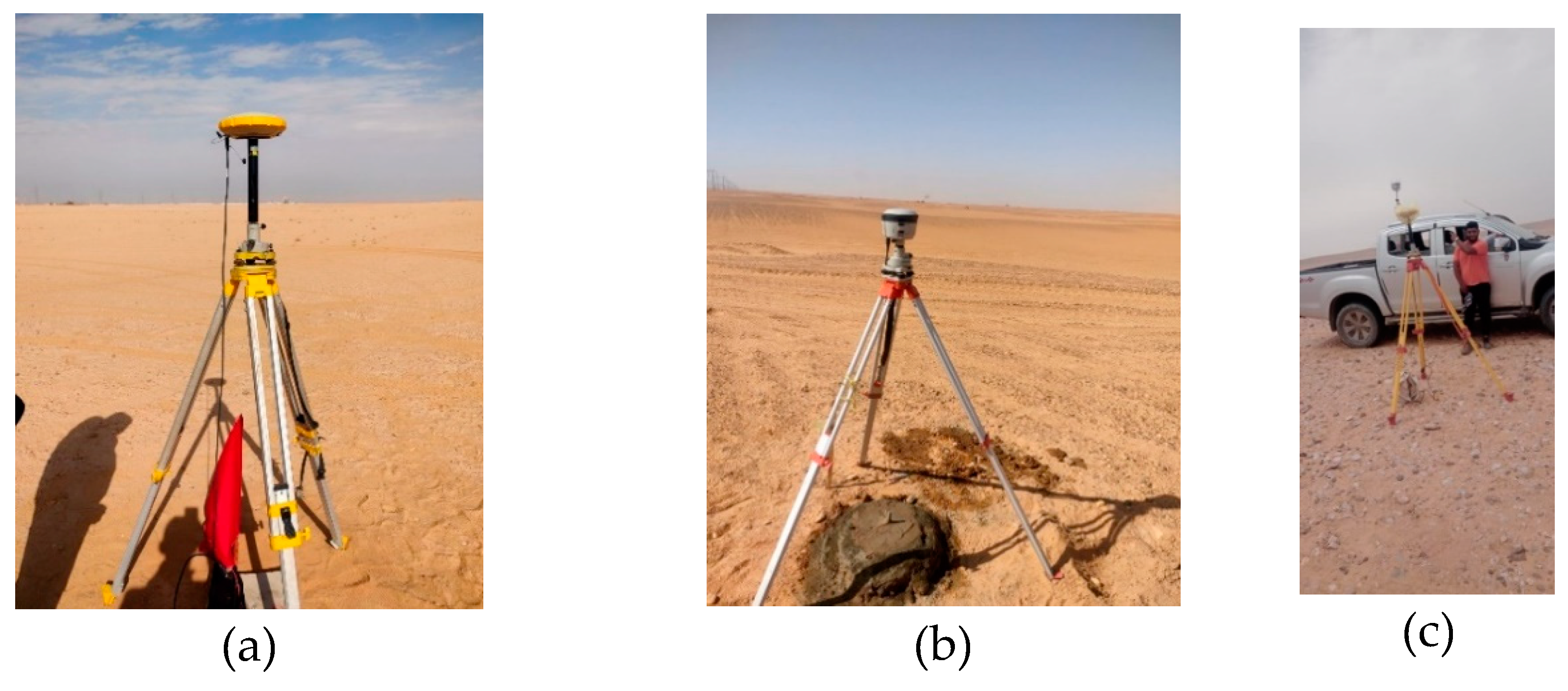
Figure 4.
Analysis flowchart.
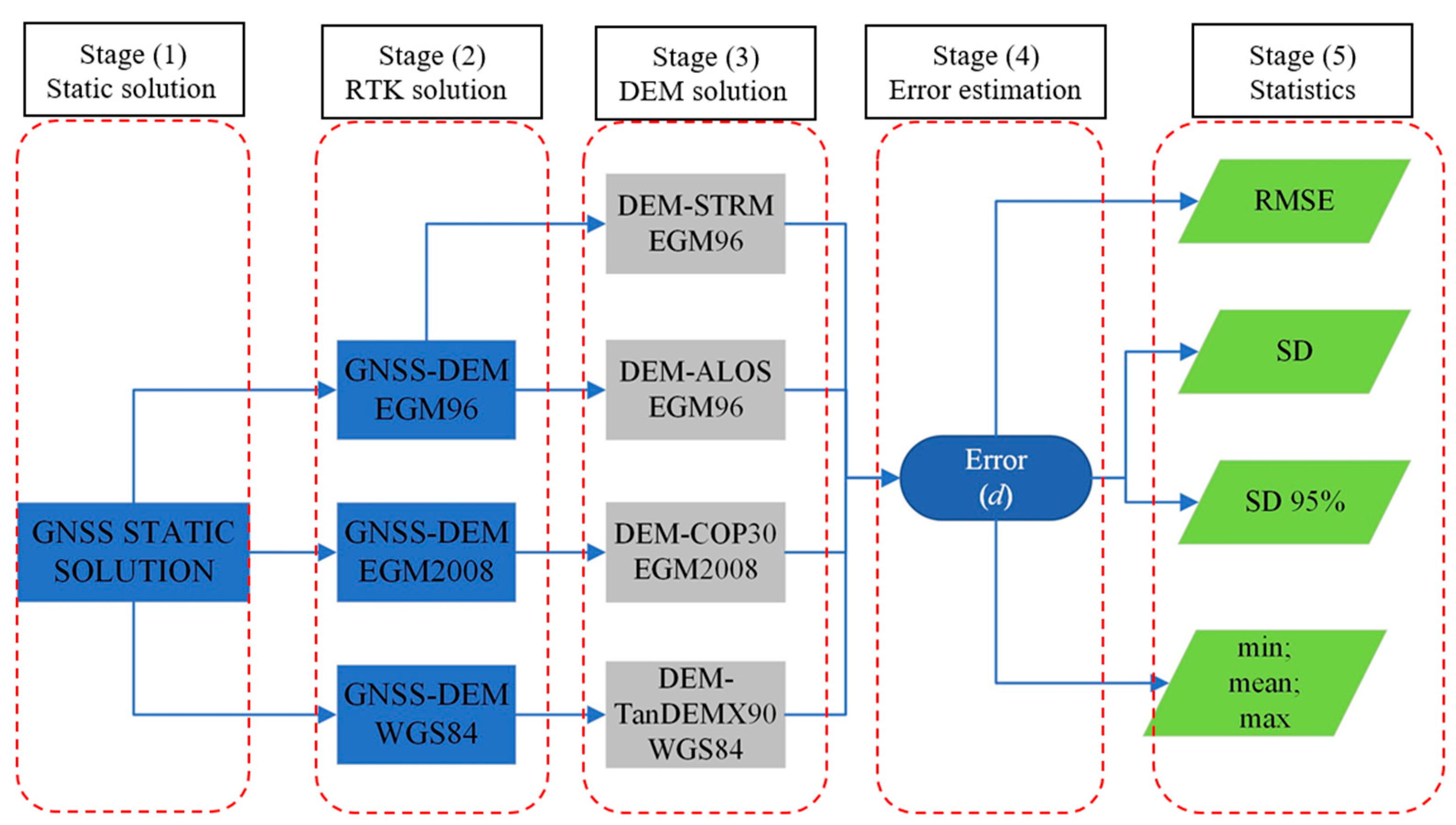
Figure 5.
Vertical error distribution for STRM, ALOS 30, COP 30, and TanDEX90 for Block I. The x-axis has been restricted from -8 m to 8 m for visualization; the y-axis is the error distribution.
Figure 5.
Vertical error distribution for STRM, ALOS 30, COP 30, and TanDEX90 for Block I. The x-axis has been restricted from -8 m to 8 m for visualization; the y-axis is the error distribution.
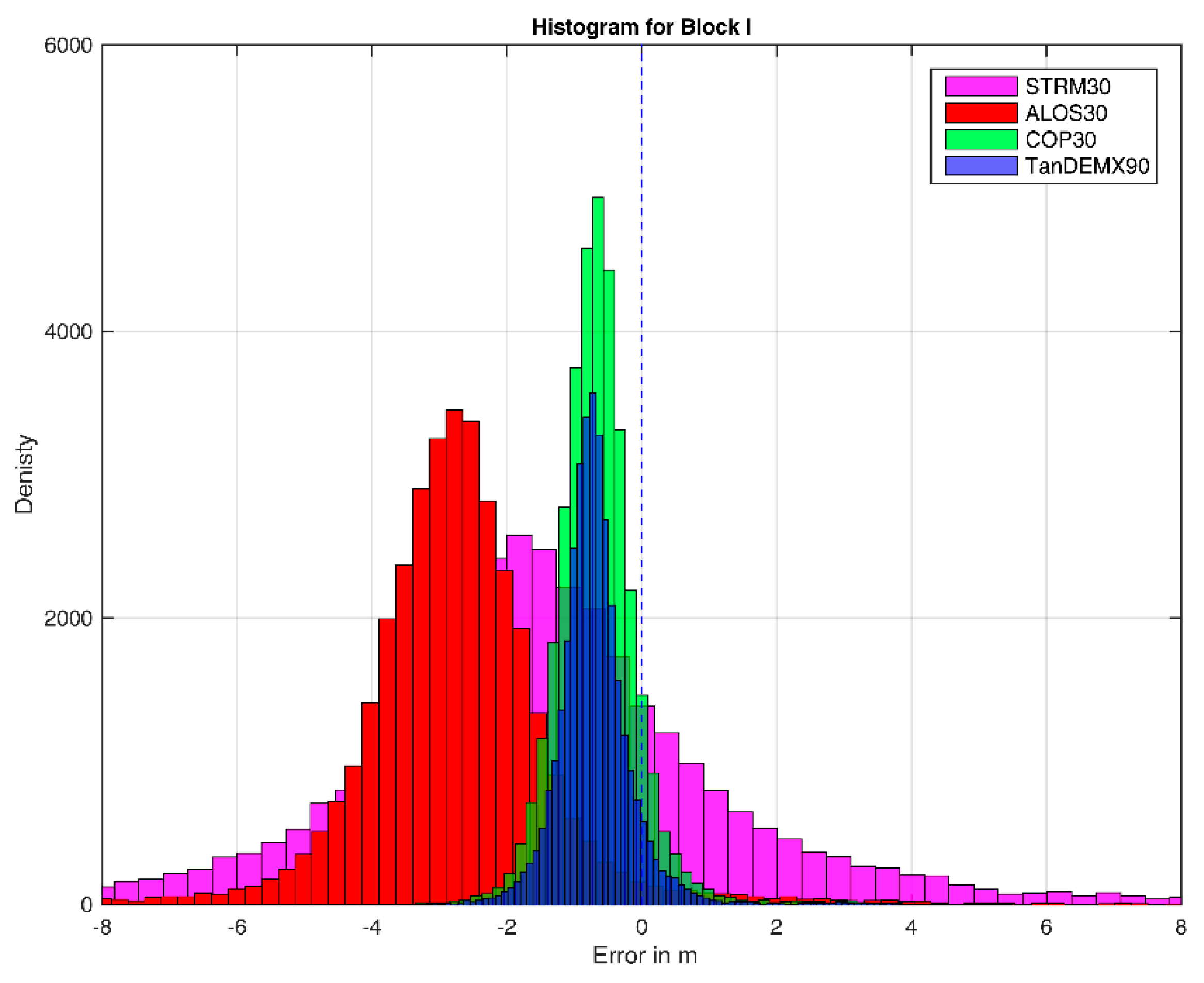
Figure 6.
Correlation between levels Using RTK Solution and Z value or Height using STRM 30, ALOS 30, COP 30, and TanDEMX90 models for block I, where the upper four graphs represent the results of correlation without filtering, and the lower four graphs represent the results of correlation with filtering.
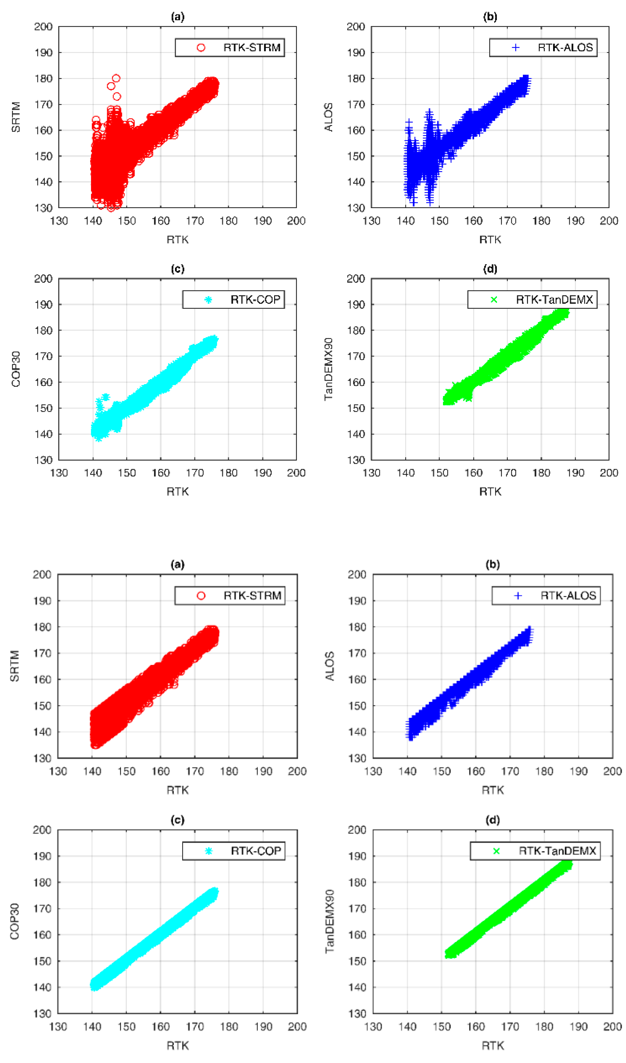
Figure 7.
Vertical error distribution for STRM, ALOS 30, COP 30, and TanDEX90 for Block II. The x-axis has been restricted from -8 m to 8 m for visualization; the y-axis is the error distribution.
Figure 7.
Vertical error distribution for STRM, ALOS 30, COP 30, and TanDEX90 for Block II. The x-axis has been restricted from -8 m to 8 m for visualization; the y-axis is the error distribution.
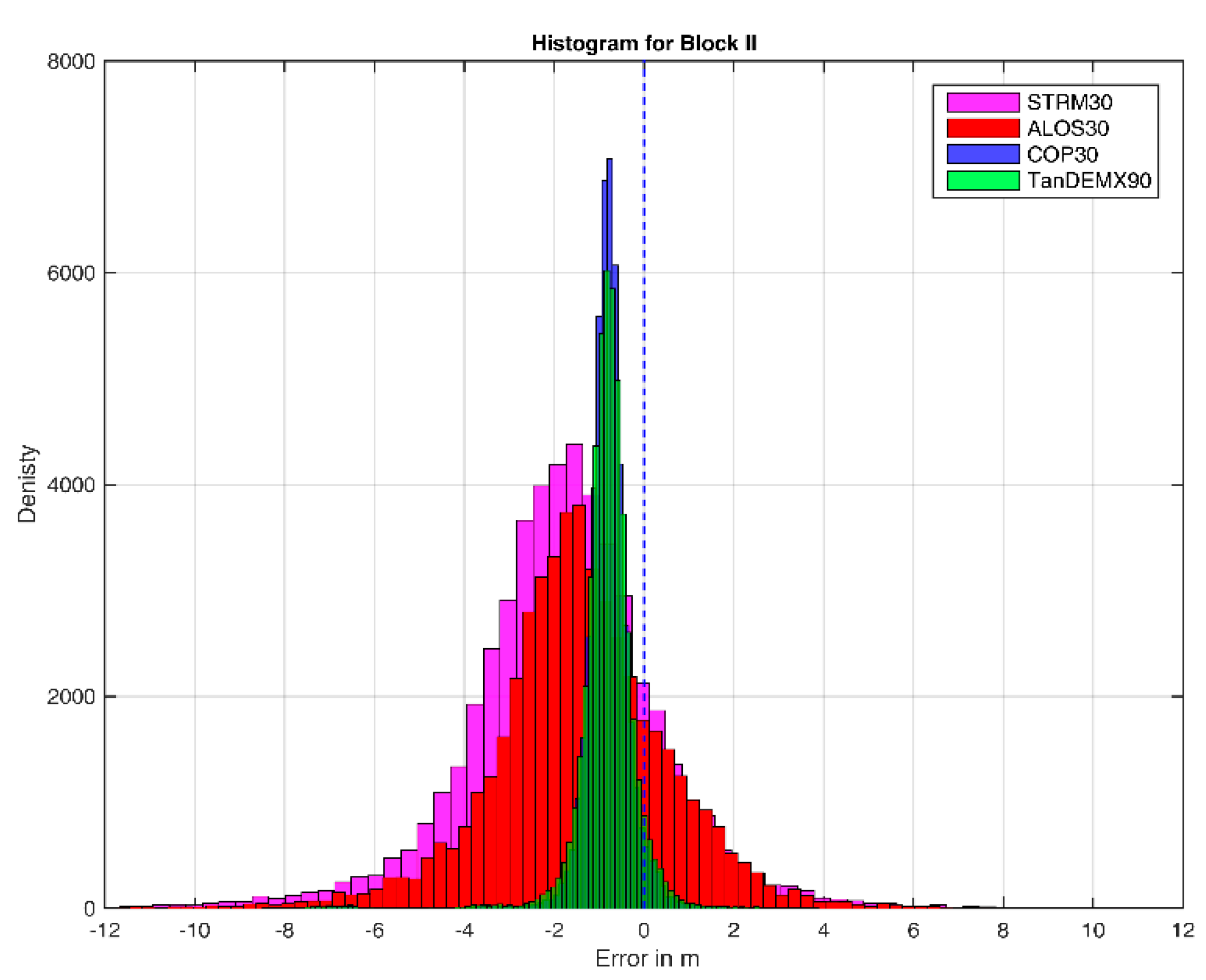
Figure 8.
Correlation between levels Using RTK Solution and Z value or Height using STRM 30, ALOS 30, COP 30, and TanDEMX90 models for block II; where the left side represents the results of correlation without filtering and the right side represents the results of correlation with filtering.
Figure 8.
Correlation between levels Using RTK Solution and Z value or Height using STRM 30, ALOS 30, COP 30, and TanDEMX90 models for block II; where the left side represents the results of correlation without filtering and the right side represents the results of correlation with filtering.
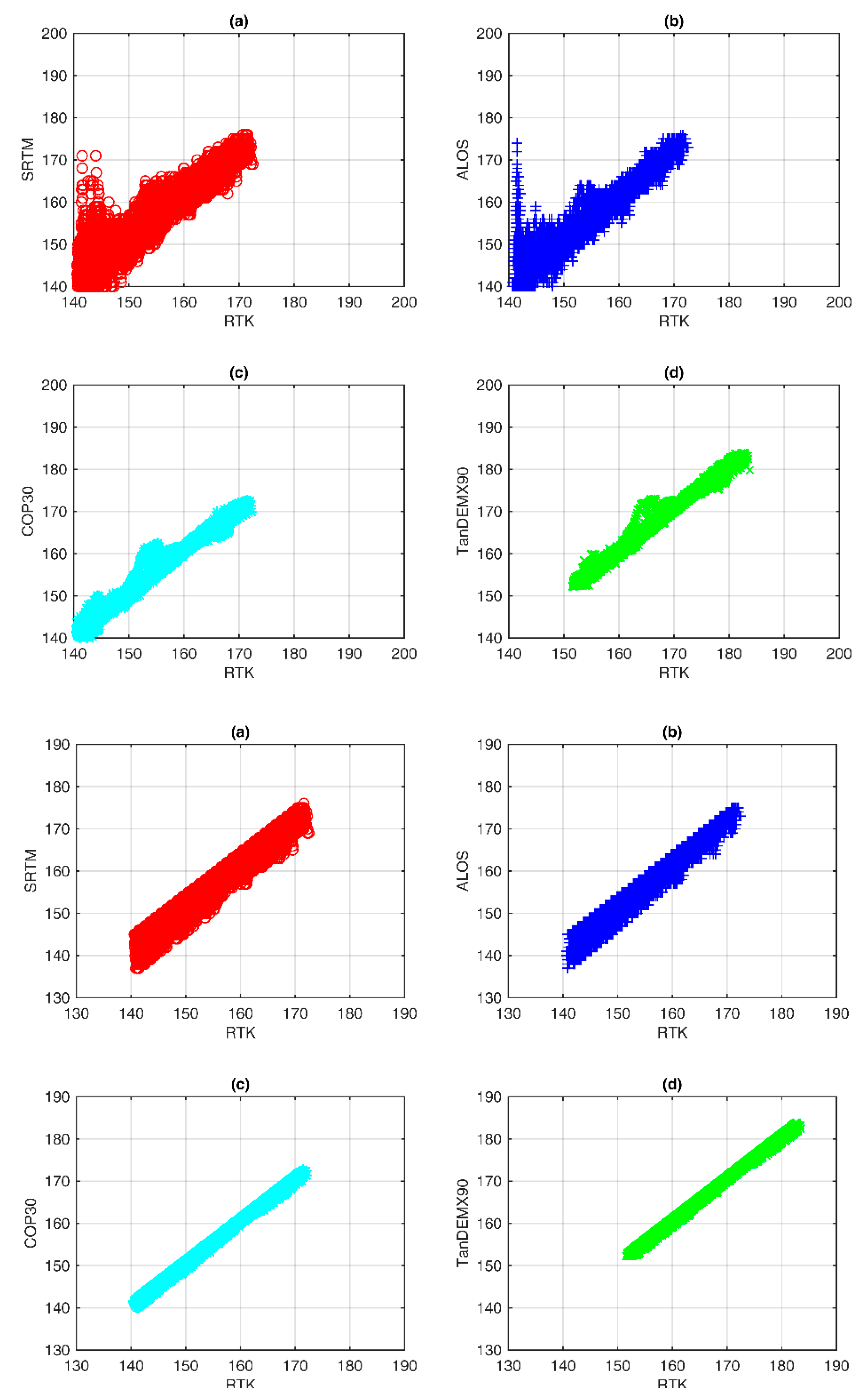
Table 2.
Absolute vertical accuracy of STRM30, ALOS30, COP30, and TanDEMX90 models for Block I.
| DEM | No. of points | RMSE (m) | SD (m) | SD95% (m) | Min (m) | ) (m) | Max (m) | R | R95% |
|---|---|---|---|---|---|---|---|---|---|
| STRM30 | 34854 | 3.59 | 3.20 | 2.26 | -33.16 | -1.62 | 21.27 | 0.9383 | 0.9702 |
| ALOS30 | 3.30 | 1.75 | 0.99 | -21.97 | -2.8 | 15.19 | 0.9702 | 0.9938 | |
| COP30 | 0.91 | 0.64 | 0.43 | -10.83 | -0.65 | 5.42 | 0.9938 | 0.9987 | |
| TanDEM-X90 | 0.90 | 0.58 | 0.38 | -4.22 | -0.69 | 5.11 | 0.9977 | 0.9990 |
Table 3.
Absolute vertical accuracy of STRM30, ALOS30, COP30, and TanDEMX90 models for Block II.
| DEM | No. of points | RMSE (m) | SD (m) | SD95% (m) | Min (m) | Max (m) | R | R95% | |
|---|---|---|---|---|---|---|---|---|---|
| STRM30 | 49471 | 2.92 | 2.27 | 1.62 | -29.48 | -1.83 | 25.39 | 0.9721 | 0.9860 |
| ALOS30 | 2.58 | 2.11 | 1.56 | -32.49 | -1.47 | 9.60 | 0.9774 | 0.9893 | |
| COP30 | 1.06 | 0.68 | 0.40 | -8.43 | -0.81 | 3.39 | 0.9974 | 0.9991 | |
| TanDEM-X90 | 1.03 | 0.62 | 0.34 | -7.84 | -0.82 | 3.87 | 0.9979 | 0.9993 |
Table 4.
The performance of the selected DEM solution in detecting the points on Block 1.
| DEM Solution | Precision | Recall | F1-Score | Support | Accuracy |
|---|---|---|---|---|---|
| GNSS-RTK | 0.999 | 1.000 | 0.999 | 34,855 | 0.98 |
| STRM30 | 0.848 | 0.498 | 0.627 | 10,400 | 0.838823 |
| ALOS30 | 0.817 | 0.532 | 0.644 | 10,400 | 0.830401 |
| COP30 | 0.834 | 0.573 | 0.679 | 10,400 | 0.839002 |
| TanDEM-X90 | 0.851 | 0.208 | 0.334 | 10,400 | 0.846778 |
Table 5.
The performance of the selected DEM solution in detecting the points on Block II.
| DEM Solution | Precision | Recall | F1-Score | Support | Accuracy |
|---|---|---|---|---|---|
| GNSS-RTK | 0.999 | 1.000 | 0.9995 | 49,472 | 0.98 |
| STRM30 | 0.800 | 0.449 | 0.575447 | 10,000 | 0.830481 |
| ALOS30 | 0.819 | 0.591 | 0.686686 | 10,000 | 0.831330 |
| COP30 | 0.793 | 0.599 | 0.682547 | 10,000 | 0.849797 |
| TanDEM-X90 | 0.820 | 0.403 | 0.540578 | 10,000 | 0.852941 |
Disclaimer/Publisher’s Note: The statements, opinions and data contained in all publications are solely those of the individual author(s) and contributor(s) and not of MDPI and/or the editor(s). MDPI and/or the editor(s) disclaim responsibility for any injury to people or property resulting from any ideas, methods, instructions or products referred to in the content. |
© 2024 by the authors. Licensee MDPI, Basel, Switzerland. This article is an open access article distributed under the terms and conditions of the Creative Commons Attribution (CC BY) license (http://creativecommons.org/licenses/by/4.0/).
Copyright: This open access article is published under a Creative Commons CC BY 4.0 license, which permit the free download, distribution, and reuse, provided that the author and preprint are cited in any reuse.


