

Submitted:
29 July 2024
Posted:
30 July 2024
Read the latest preprint version here
Abstract
Traditional urban design often overlooks the synchronisation of human and ecological connectivities, typically favouring corridors for ecological continuity. Our study challenges this convention by introducing a computational design approach, Meta-Connectivity, leveraging the deep generative models performing cross-domain translation to integrate human-wildlife landscape connectivity in urban morphology amidst the planetary urbanisation. Utilising chained Pix2Pix models, our research illustrates a novel meta-connectivity design reasoning framework, combining landscape connectivity modelling with conditional reasoning based on deep generative models. This framework enables the adjustment of both human and wildlife landscape connectivities based on their correlative patterns in one single design process, guiding the re-materialisation of urban landscapes without the need for explicit prior ecological or urban data. Our empirical study in East London demonstrated the framework's efficacy in suggesting wildlife connectivity adjustments based on human connectivity metrics. The results demonstrate the feasibility of creating an innovative urban form in which the land cover guided by the connectivity gradients replaces the corridors based on simple geometries. This research thus presents a methodology shift in urban design, proposing a symbiotic approach to integrating disparate yet interrelated landscape connectivities within urban contexts.
Keywords:
urban design
; deep generative models
; cross-domain translation
; landscape connectivity
; progressive reasoning
; urban ecology
1. Introduction
1.1. Significance of Landscape Connectivity to Urban Ecology
Landscape connectivity (Spear et al., 2010) is a spatial metric referring to the degree to which the landscape facilitates or impedes movement among resource patches. It encapsulates the complex interplay between the landscape’s spatial attributes and its biological makeup, shedding light on how it either facilitates or constrains organism movement and interaction. Traditional spatial planning methods often rely on corridors to maintain ecological connectivity. These corridors are usually designed to connect protected areas or natural habitats to promote species migration and gene flow (Aziz & Rasidi, 2014; Hilty et al., 2020).
However, such approaches may overlook the impact of human landscape connectivity, including factors like urbanisation and transportation network development on ecological connectivity. This oversight is evident in existing literature, where human landscape connectivity is seldom assessed and rarely considered alongside wildlife landscape connectivity within the same project. Ideologically and methodologically, humans are often assumed to be external to local ecologies, positioned as counterparts to wildlife.
Our research seeks to bridge the divide between traditional ecology and human geography by integrating wildlife landscape connectivity with human landscape connectivity using deep learning algorithms capable of cross-domain translation (Gonzalez-Garcia et al., 2018). This study, by challenging conventional planning approaches that largely employ corridors, may foster discussions on environmental justice (Ali & Kamraju, 2023; Chang & Liao, 2011): the equitable distribution of ecological resources and fair access to natural resources for different species and human populations. By merging both types of connectivity at an operational level, this research aims to explore a new method of urban landscape planning. In this approach, new urban forms are anticipated to emerge to accommodate the synergistic effects between local ecological networks and human activities, where conflicts between human activities and wildlife habitats are mediated through the re-materialisation of urban structures (Brenner & Schmid, 2017).
1.1.1. Cross-Domain Translation and Conditional Design Reasoning
Cross-domain translation (Gonzalez-Garcia et al., 2018) is a process that involves the transference and mapping of patterns or features from one domain to another. In such a process, knowledge learned from one data distribution (source domain) are applied to a different but related data distribution (target domain), transforming inputs from the source domain into equivalent outputs in the target domain while preserving intrinsic properties and adapting to the target domain's features (Zhou et al., 2023).
Pix2Pix, since its inception, has been extensively applied by architects for conditional reasoning: it is used to test models trained on design conditions from the source domain to generate new data belonging to the target domain. This form of reasoning offers a viable path for problems where the relationship between two factors is inscrutable and hence cannot be addressed through traditional deductive design reasoning. Examples include the facade generation by Isola et al (2017)., residential plan generation by Huang et al (2018)., and spatial organisation studies by Yu (2020). Similar technologies have also expanded the scope of cross-domain translation in design applications. The advent of CycleGAN (Zhu et al., 2017) made unpaired data translation feasible. Examples include the conversion between architectural sketches and photo-realistic renderings (Li & Xu, 2022), and the transformation between bump maps and hyperbolic images (Hassab et al., 2021), demonstrating the translation between a set of concepts based on a vast array of cases and another set. Nvidia's GauGAN series (Park et al., 2019a, 2019b; Salian, 2019) applied cross-domain translation to digital sketchpads, converting real-time sketch inputs and text inputs into corresponding photo-realistic images.
Furthermore, there are efforts to utilise a series of domain-to-domain models in sequence to address complex design problems composed of multiple problem layers. Each problem layer is treated as a relevant combination of two domains for conditional reasoning. This condition involves mapping a given design premise to the conclusive schema of the previous layer. Chaillou employed a model called ArchiGAN (Chaillou, 2019) for sequential reasoning across multiple domains to generate architectural plans, from building contours to interior details. Similarly, Chan and Spaeth (2020) attempted to create a transformative loop between two cGANs for architectural sketches and images, mimicking the visual reasoning pattern of architects .
In summary, this technique has demonstrated its capability in integrating disparate yet related concepts in the design process. However, there is a notable scarcity of empirical works exploring its potential in synthesising different spatial metrics. This study will build upon this foundation with a hypothesis that landscape connectivity pertaining to different objects can be concurrently considered within the same design process, seeking a symbiotic design approach.
1.2. The Meta-Connectivity Hypothesis
Studies like pattern theory and its applications (Bhatt, 2010; Alexander, 1974) suggest that there are usually conflicts between human spatial connectivity and wildlife spatial connectivity in an urban area. However, such conflicts are not comprehensive; they sometimes antagonise each other and sometimes attract each other. In cities, it is common to witness crowded empty spaces with plentiful pigeons and other small animals gathering, and countless cases show that the movement of humans has driven out the colonisation of wildlife species. Such conflicts must be addressed in a redesign process to identify the correct spatial pattern, but the question remains: how can this be achieved?
The present study formulates a novel theory of meta-connectivity, serving as a hypothesis, which integratively considers two pivotal variables: the spatial connectivity of both humans and wildlife - two entities traditionally analysed in isolation. This theoretical framework elucidates a causal correlation between the spatial interconnectedness of humans and their wildlife counterparts. Hence, it facilitates the application of conditional reasoning to predict emerging spatial connectivity patterns within wildlife populations. Building upon this concept of causal reasoning, conditional generative models are considered the optimal technical approach where the status of human spatial connectivity can lead to a corresponding and predictable state of wildlife spatial connectivity, and vice versa.
2. Material and Methods
2.1. The Meta-Connectivity Framework
Existing research indicate a discrepancy between human and wildlife landscape connectivity, which can manifest as mutual aversion or attraction. This concept is resonated in the pattern analyses by Batty (1974) and Lystra (2017), who demonstrate that each form of connectivity can be conceptualised as a distinct 'image.' The differences and conflicts between these forms of connectivity can be characterised by specific feature distributions and analysed using computer vision techniques.
Inspired by such a methodology, we propose an innovative, image-based approach within our study, wherein we introduce deep generative models to perceptual signal processing and content generation into a computational meta-connectivity reasoning framework (Figure 1). The aim of the framework is to employ deep generative models trained with valid reference data to simultaneously fine-tune the state of landscape connectivity for both humans and wildlife species through the effect of cross-domain translation, and based on this, to renovate the local landscape materiality.
2.2. Study Area
The project focuses on a one-kilometre square site in Limehouse, East London, defined by the geolocations (51°30’21.7”N, 0°01’48.9”W), (51°30’54.0”N, 0°01’48.9”W), (51°30’21.7”N, 0°00’56.9”W), and (51°30’54.0”N, 0°00’56.9”W). The site’s climate is classified as Cfb (marine or oceanic) according to the Köppen-Geiger Climate Classification (Peel et al., 2007). The National Biodiversity Index (NBI) values range from 0.400 to 0.500. Figure 1 provides a preliminary exploration of the spatial connectivity conflicts between humans and wildlife.
To mitigate the potential bias associated with geopolitically defined study areas, the resistance mapping was extended 10 km into the peripheral regions surrounding the study area to increase the spatial coverage. This approach (Gurrutxaga et al., 2010) enhances the understanding of the study region’s biological connectivity. Extending the map beyond traditional boundaries ensures more comprehensive representation and bolsters result reliability.
2.3. Data Collection
Connectivity modelling relies heavily on the choice of datasets. This study employs two distinct datasets, the National Biodiversity Index (NBI) and eBird data, which capture detailed aspects of terrestrial and avian biodiversity, respectively, to ensure the validity of the research. This approach is also anticipated to uncover the importance of data subjectivity and the resulting variations in outcomes it may cause. It will aid in providing comprehensive insights into the connectivity of various species and demonstrate how deep generative models can be effectively trained using strategically curated 'valid knowledge'.
2.3.1. Landscape Connectivity on NBI Data
NBI quantifies species diversity within a specified area. As delineated by the American Museum of Natural History, the Biodiversity Index is determined by dividing the number of species by the total individuals across all species in the area (American Museum of Natural History, 2001). It is essential to recognise that ‘area’ embodies varied spatial dimensions, from countries (National Biodiversity Index) to cities (City Biodiversity Index) (Delbaere, 2002; Han et al., 2020). For this analysis, NBI data reflects estimations of richness and endemism across four terrestrial vertebrates and vascular plants. Index values span from 0.000 to 1.000, with elevated values indicating heightened biodiversity (Jepson et al., 2015). To train the Pix2Pix models, 120 examples were chosen from the Cfb region (Delbaere, 2002), where London is situated. The selection process ensured that each example presented higher NBI values to the study site, ensuring the model learned knowledge that suggest superior biodiversity.
2.3.2. Landscape Connectivity on eBird Data
Alternatively, this study utilises a connectivity dataset focused on bird species, which is dominated by the eBird metric. 120 exceptional examples have been selectively sampled from this dataset in the Cfb area, which are of the same scale (1km*1km) as the site. The eBird database (Auer et al., 2022) is a collaborative effort managed by the Cornell Lab of Ornithology and is based on human observations from experts in various fields worldwide. The team works to increase data volumes and enhance the quality of the quantitative data. The eBird data captures the occurrence and contextual information of bird sightings and is visually represented as scatter plots.
2.4. Modelling Landscape Connectivity
Modelling landscape connectivity in ecological contexts involves several approaches, with circuit theory being paramount (Dickson et al., 2019; Hall et al., 2021; McRae et al., 2008b; Shah & McRae, 2008). Tools like Circuitscape blend graph theory with electrical circuit theory to measure habitat connectivity, requiring a resistance surface as an essential input. This surface is a pixelated representation reflecting the movement cost through the landscape. Appropriate resistance values can be determined from models examining the link between resistance values and species habitat (Belote et al., 2022; Braaker et al., 2014; Carroll et al., 2020).
Our wildlife movement resistance settings utilised studies on large and medium-sized mammals (Gurrutxaga et al., 2010), Lynx (Hetherington & Gorman, 2007; Hetherington et al., 2008; Özcan & Erzin, 2020), Wolverine (Carroll et al., 2020), and Moose (Batha & Otawa, 2013). The credibility of these settings was verified by expert consultations and by comparing simulation results with observed data (Table 2).
For urban-scale simulations, solely incorporating land-use attributes can lead to inaccuracies (Batha & Otawa, 2013). To improve this, we integrated land use, roads, rivers, and specific building layouts, optimising resistance calculations for animal movement. Two factors were merged into a raster map using ArcGIS weight overlay function, assigning equal weights of 0.5, ensuring data’s scientific integrity.
Utilising circuit theory, we quantified human movement as resistance values, building on Howey’s (2011) findings that it models human spatial movement. We integrated the attraction of Points of Interest (POIs) to orientation-destination in the gravity model with humans’ tendency to move specific distances from their start (Barbosa et al., 2018; Wang et al., 2023). We hypothesise that dense POI clusters both attract and repel individuals during commutes. Thus, in the circuit method, we consider the POI cluster as the starting point and an area of high resistance based on activity radius distribution (Table 2). Utilising ArcGIS 10.2, we reclassified the raster per resistance settings, integrating local and city-scale layers for human and animal mobility. Rivers were deemed impassable for humans. Converted resistance maps to ASCII rasters, and computed mobility probabilities with Circuitscape 4.0 (McRae et al., 2008a), visualised through QGIS 2.18.

Table 1.
Resistance settings for landscape connectivity modelling on wildlife and human factors.
| Factor (wildlife) | Sub-factor | Resistance value (ours) | Resistance value (Gurrutxaga et al., 2010) | Resistance value (Özcan & Erzin, 2020) | Resistance value (Batha & Otawa, 2013) | |
| Local scale | Buildings | with buildings blocking | 1000 | / | / | 500 (maximum 500) |
| without buildings blocking | 100 | / | / | 100 (minimum 100) | ||
| City scale | Land use | Urban | 1000 | 1000 | 1000 | 500 |
| Industrial | 1000 | / | 1000 | 500 | ||
| Water | 100 | 100 | 1000 | 100 | ||
| Quarries | 100 | 90 | 1000 | 250 | ||
| Crops | 60 | 60 | 60 | 400 - 500 | ||
| Grassland | 40 | 30 - 40 | 40 | 100 - 500 | ||
| Forest | 10 | 1 - 20 | 10 | 100 | ||
| Roads | <1000 vehicle/day | 80 | 80 | 80 | / | |
| 1000-5000 vehicle/day | 100 | 100 | 100 | / | ||
| 5000-10000 vehicle/day | 300 | 300 | 300 | / | ||
| 10000-20000 vehicle/day | 700 | 700 | 700 | / | ||
| >20000 vehicle/day | 800 | 800 | 800 | / | ||
| Distance to road: 0.4km | / | / | / | 250 | ||
| Distance to road: 0.8km | / | / | / | 500 | ||
| Rivers | Large river (>30m width) | 120 | 120 | 120 | / | |
| Medium river (<30m width) | 40 | 40 | 40 | / | ||
| Distance to Stream: 0.8km-3.21km | / | / | / | 100 - 300 | ||
| Distance to Stream: 3.21km-9.65km | / | / | / | 300 - 500 | ||
| Factor (human) | Sub-factor | Resistance value (ours) | ||||
| Local scale | Buildings | with buildings blocking | 1000 | |||
| without buildings blocking | 100 | |||||
| City scale | Kernel density of poi aggregation (Search radius) | 0-25m | 1000 | |||
| 25-50m | 500 | |||||
| 50-100m | 200 | |||||
| 100-200m | 100 | |||||
| 200-300m | 60 | |||||
| 300-800m | 40 | |||||
| >800m | 10 | |||||
| Roads | <1000 vehicle/day | 80 | ||||
| 1000-5000 vehicle/day | 100 | |||||
| 5000-10000 vehicle/day | 300 | |||||
| 10000-20000 vehicle/day | 700 | |||||
| >20000 vehicle/day | 800 | |||||
| Rivers | Large river (>30m width) | 1000 | ||||
| Medium river (<30m width) | 1000 | |||||
Notes: higher values = higher resistance.
2.5. Analytical Metrics of Dataset Processing
Three distinct metrics are employed in the process of dataset profiling: 1) the overall connectivity metric (Cm), 2) the kernel connectivity vitality (Vk), 3) and the histogram of oriented gradients (HOG). They respectively visualised the spatial features of human landscape connectivity (LCh) and wildlife landscape connectivity (LCw), as well as their spatial distribution, for assessment during the research process.
First, the overall connectivity metric (Cm) is vital in understanding the comprehensive landscape connectivity across the entire sample territory. Although it might not fully depict the local ecological quality, it provides theoretical insights into the same. Second, the kernel connectivity vitality (Vk) allows for the investigation of specific locations of observed wildlife, portrayed through a scatter plot representation. This method utilises raw data from eBird, represented by scatter points marked on a map, enriching the analysis of both the NBI and eBird datasets. Third, the histogram of oriented gradients (HOG) is employed to discern variations in spatial connectivity features engendered by the proposed urban landscape. The HOG calculation (Dalal & Triggs, 2005) adopts a nested kernel method, encompassing two different kernel levels, namely, the blocks and the interspersed cells (Table A.1).
2.6. Dataset Observations
2.6.1. The Testing Site
The site is bordered by open spaces, including parks and waterways, with a canal on its western side connecting to the Thames River. Typical riparian parks along the riverbanks act as ecological corridors (Figure 2a). The site’s central area features east-west ecological corridors aligned with transportation infrastructure, prominently depicted in the HOG image.
As illustrated in the HOG image (Figure 2b), several ecological hotspots with high spatial connectivity surrounding the site are not effectively connected by the planned ecological corridors. The site’s central area exhibits pronounced linearity. There is minimal transition in the spatial connectivity gradient in the horizontal (east-west) direction, while the two sides of the edge (north-south) exhibit extremely strong gradient transitions. In other directions, the degree of gradient change remains underdeveloped, except for the horizontal direction. These phenomena suggest that the corridor’s geometry is prominently presented, and the space along the north-south direction contains distinct markers that segregate natural areas from non-natural ones. In addition, these strong edge effects raise questions about the role of corridor connectivity in linking ecological nodes within the region. The connectivity between many nodes, such as Mile End Park and other nodes, does not exhibit significant recognisable transitions.
The present overall connectivity (Cm) of the location is 118.03947448730469 for humans and 111.12281799316406 for wildlife. The variance of its HOG is 0.007228746. As of June 23, 2022, there are no eBird observation records on the site. Based on this fact, its kernel vitality Vk is tentatively calculated as approaching 0.0.
2.6.2. Data Evaluation
Compared to the NBI group, the HOG values of the images in the eBird group exhibit greater overall dispersion (Table 3) (Figure 3 and Figure 4). Moreover, individual instances within this group manifest distinct spatial variations in connectivity and orientation. The correlation between HOG Variance and Vk (wildlife) is minimal, suggesting they are largely independent. This means that anisotropy changes in landscape connectivity do not significantly influence bird observation frequencies at specific locations. However, a discernible moderate positive correlation exists between Cm and Vk. Notably, a moderate negative correlation between HOG Variance and Cm suggests that areas with heightened connectivity exhibit more consistent spatial anisotropy changes, largely uninfluenced by dominant directional spatial elements, such as corridors.
2.6.3. Metric Biases
The NBI index, solely based on species numbers, overlooks the size of natural areas and habitat authenticity. Consequently, there can be counterintuitive results. For instance, despite their vast semi-natural expanses and renowned ecological conservation (Magnussen & Dombu, 2019; Rugg, 2016), Scandinavian countries rank lower on the index.
3. Architecture of Reasoning System
3.1. Conditional Generative Model: Pix2Pix
In light of the meta-connectivity challenge undertaken by this research, a conditional generative adversarial network (cGAN) algorithm is required to provide an ‘even field’ (del Campo et al., 2019) to simultaneously address diverse landscape connectivities. It accomplishes this through a cross-domain translation approach, treating human landscape connectivity and wildlife landscape connectivity as a pair of causally-linked problem domains to enable causal reasoning, given design conditions such as a specified human lan dscape connectivity.
In this research, we utilise Pix2Pix models to undertake such tasks. Pix2pix is the cGAN architecture usually trained by paired image data for conditional image-to-image translation that has demonstrated its competency in this regard and was hence widely adopted. It employs a generator for image creation and a discriminator to ensure the result matches the desired condition. A Pix2Pix model is trained using an adversarial loss function, which consists of two parts: the loss for the discriminator, , and the loss for the generator, .
The loss for the discriminator, , is defined as (6):
where is the input image from domain X, is the corresponding target image in domain Y, is the output image generated by the generator, and represents the discriminator’s output when given the input image and target image. The expectation E is taken over the distribution of the training data.
The loss for the generator, , is defined as (7):
where is the output image generated by the generator and represents the discriminator’s output when given the input image and generated image.
The overall loss function, , is the sum of the losses for the discriminator and generator:
The generator and discriminator are trained alternately, with the generator trying to minimise the overall , and the discriminator trying to maximise it. The training process continues until the generator produces outputs that are indistinguishable from real images according to the discriminator (Figure 5).
3.2. Progressive Reasoning
In the meta-connectivity hypothesis, designs spanning multiple domains (here, human landscape connectivity, wildlife landscape connectivity, and materiality) surpass the capabilities of a standard conditional generative adversarial network (cGAN) model. This is due to its intrinsic limitation of reasoning across only two domains (Mirza & Osindero, 2014). To address this, the progressive reasoning approach, which employs a series of concatenated cGAN models to incrementally solve a complex problem, is invented to address the issue. The approach effectively enhances connectionist design cognition by dividing manifold reasoning processes into two-domain tasks tackled by individual cGANs. It has gained prominence in architectural research post-2017, with projects like ArchiGAN and Glitch-Arch employing it for causal reasoning across correlated domains using representational data (Chaillou, 2019; Yu, 2020).
In ArchiGAN (Chaillou, 2019), for example, a chain of three cGANs advances from a site outline through domains, including figure-ground and program-based plan segmentation, culminating in the generation of a building plan. While the relationship between the site outline and building plan is implicit and not directly observable, progressive reasoning bridges these domains. In our project, we adopt a dual Pix2Pix model structure for correlation analysis across domains including human landscape connectivity, wildlife landscape connectivity, and materiality. Our aim was to re-materialise the landscape based on those varied conductivities.
3.3. Training Pix2Pix Models
Informed by the Anthropocene theory, this project acknowledges the importance of human spatial connectivity in design solutions. The design process must account for the existing urban fabric and its inherent social dynamics. The ultimate aim of this reasoning task is to predict the materiality of the landscape through machine learning, ensuring desired landscape connectivity for both humans and wildlife.
To achieve this, the objective is to create a landscape image that reflects the desired human-wildlife connectivity and maximises human landscape connectivity. This paper explores the use of conditional generative adversarial networks (cGANs) to facilitate this, utilising a tandem of two Pix2Pix models that translate between connectivity and latent materiality. The first Pix2Pix model is trained on the human landscape connectivity (LCh) and wildlife landscape connectivity (LCw) datasets, forming the implicit knowledge of the relationship between human and wildlife spatial affordance at a location. With this knowledge, the model can suggest a landscape connectivity condition for local wildlife (LCw’) based on the given human landscape connectivity. The second Pix2Pix model, trained on LCw and satellite images, then generates a materiality suggestion informed by LCw’. Both models are trained for 1000 epochs (Figure 6).
Both the Pix2Pix models adopt TensorFlow 2.9 framework and were trained for 1000 epochs; the hyperparameters were carefully tuned for high-quality output (Table 4).
4. Results
In the quest to understand the relationship between input and target images, this study employs the Pix2Pix deep learning model. Leveraging the causal relationship between input and target images, the study decodes the patterns and interdependencies governing the spatial connectivity between humans and wildlife and use them to create new urban landscape.
4.1. Summary of Results
4.1.1. General Observations
The territories exhibiting the highest degree of connectivity (indicated in bright yellow) remain largely unchanged, while those with moderate connectivity (indicated in orange) permeate the building blocks and segment the building territories. The spatial segregation between human and non-human territories is significantly blurred.
For wildlife landscape connectivity LCw, we studied both NBI and eBird groups. The NBI group’s urban fabric, especially its road network, portrays a regular pattern, with broad streets influenced by underlying data’s anisotropy variance. The river sections show low wildlife connectivity, and a green space proposal will replace the riverbank to increase LCw values. This redesign subtly alters roads and building structures. In contrast, the eBird group reveals high connectivity near Chrisp Street Market and regions around A1203. This group’s landscape incorporates a pronounced ecological patchwork, where an urban green belt obscures road grids, suggesting diminished vehicular movement. This greenery lacks definitive boundaries, and building structures are more intertwined with natural elements. Both groups advocate for high LCw landscapes around riverbanks and Westferry Station, while mid-range LCw dominates architectural zones. Unique building geometries and porous edges facilitate ecological diversity. Bartlett Park’s size reduction is recommended, with its southern section undergoing a community-integrated texture transformation. The results culminate in an urban space where the demarcation between human and wildlife territories is blurred. This blending permits diverse architectural solutions, fostering equitable access to natural zones and suggesting versatile land usage. Overall, rigid wildlife corridors transition into porous, wildlife-friendly structures, seamlessly integrating nature into urban design.
The proposed materiality map, independent of the semantic information from the satellite image, offers a space for creative interpretations. For example, the white and light grey pixels typically representing building roofs are shown to encompass regions blending human-oriented areas with elements that challenge the conventional building grid, fostering coexistence with wildlife. Many human territories, including streets and buildings, are proposed to undergo diverse reconfigurations (Figure 7 L1).
The parametric adaptation approach enables a variety of architectural solutions to be implemented. As illustrated in Figure 7, the rematerialised urban space blurs the material-typological boundaries between human and wildlife territories, nearly to the point of disappearing. This promotes multiple modes of access for humans to the territories accommodating wildlife, implying the agility of land use and the potential for innovative programming. The boundarylessness of the materiality scheme fosters the equal accessibility of natural territories for the general public.
4.1.2. Variational Analysis: Informing Following Design Process
In the second Pix2Pix model, the generated landscape materiality images are treated as a matrix, where the colour values of each channel represent the materiality vectors. The vectors serve as references for urban surface re-materialisation, not representing specific materials. The difference (distance) in pixel values between the original landscape materiality maps and those from the Pix2Pix model is termed an anisotropy. This difference guides the re-materialisation process and is used as a maxel field for deploying new material change units, which include both materials and forms. Importantly, these units renovate without discarding original local artifacts, respecting existing architectural conditions and aiming to reshape local landscape connectivity.
Pixel-wise Cosine distance is measured between the suggested landscape image in RGB mode and the satellite image, serving as materiality guidance for subsequent design actions (Neto et al., 2010). The distance for each reference sample is defined as follows:
The distance map guides the parametric model to regenerate the urban fabric based on a parametric approach, adhering to the given landscape condition. Territory units are segmented using the k-means algorithm, accounting for materiality distances and human landscape connectivity. The data features are represented by r, g, b pixel values. Using the elbow method (Syakur et al., 2018 ), we set k to 4 to categorise the territorial units on a high-low gradient, though this can be adjusted for deeper analysis (Figure 8). In the generative system, each cluster corresponds to a parametric prototype that refines the urban fabric by varying space-sharing intensities.
4.2. Reviewing Generated Outputs
4.2.1. General Observation
Throughout the entire design process, some common phenomena can be observed across all outputs. As evidenced in the LCw’ created on both datasets, the territories with the highest connectivity (bright yellow) remain relatively unchanged, whereas the moderate connectivity (orange) permeates the building blocks and segments the building territories. Furthermore, these territories form smaller, directional, or softer connectivity gradients. The spatial segregation between human and non-human territories is significantly blurred.
The suggested materiality map is detached from the semantic information from the source, the satellite image of the site. An interpretation space is thus created to allow creative interpretations. For example, most of the white and light grey pixels in the satellite image represent the building roofs and other hard surfaces, whereas they turn out the cloudy territories holding several human-interested areas and the granulated spray blended with the green elements to deconstruct the building grides which mean to exclude wildlife. We can also find a large number of human territories including streets and building surfaces are suggested to be reconfigured in such mixtures, in various proportions (Figure 6 and Figure 7).
4.2.2. Searching the Best Fit of the Targeted Landscape Connectivity Model
The inherent variability in neural networks primarily stems from the random initialisation of their plentiful parameters. This, combined with the fitting process in machine learning, results in a scenario where training multiple identical neural network models with the same dataset and hyperparameter configuration will invariably lead to the generated outputs that are never exactly the same (with the probability of repetition so low as to be negligible). Consequently, multiple training in parallel can provide variation and selection, which is advantageous for decision making. Under this hypothesis the present study conducted four separate training sessions for the Pix2Pix model respectively using both the NBI and eBird datasets (Figure 9). Each output suggests a unique LCw’ condition.
According to the analysis in the data processing, it is known that HOG variance V and overall landscape connectivity Cm are correlated at an observable degree. Subsequently, this study employs linear regression on these two variables separately for the NBI and eBird groups’ LCw’ prediction images. The regression model represents the ‘good ecological connected landscape’ model presented by the datasets. By observing the absolute value of the distance between the regression model predicted HOG variance and the measured HOG variance for each LCw’ candidate. the one having smallest distance can be interpreted as the best match.
In the NBI group, the most congruent value to the linear regression model prediction is found in NBI_LCw’_0.png, with a mere discrepancy of 0.0000594910. Meanwhile, in the eBird group, eBird_LCw’_3.png exhibits the closest resemblance to the predicted V value, presenting a deviation of 0.0005037503 (Table 5). Consequently, these two images are selected as LCw’, serving as the conditional images for the second Pix2Pix model, to conduct landscape materiality inference (Figure 10 and Figure 11).
5. Discussion
5.1. Main Findings
5.1.1. Redefining Urban Nature with Meta-Connected Morphology
The findings illustrate a shift towards a non-standardised urban spatial form, characterised by rich porosity and detailed intricacies. Within this evolved framework, complex and nuanced transitions occur between natural elements and human habitations. Such novel spatial forms differentiate the results from the existing urban spatial morphology. Urban nature, along with its defining mechanisms, is redefined within the new urban landscape.
Matias Del Campo has previously noted the dematerialisation effect inherent in connectionist generative models during mapping (del Campo et al., 2019). In contrast, our study harnesses this effect, seeking to enact re-materialisation of the site by identifying the materiality state corresponding to the target landscape state. The urban space, when reconfigured, nearly erases the material-typological boundaries between human and wildlife territories, leading to an almost seamless blend. This lack of demarcation encourages diverse ways for humans to access spaces that wildlife inhabits, signifying both the adaptability in land use and the prospect of creative programming. With minimised divisions in the materiality scheme, it ensures that natural territories are accessible equitably to all, thereby accentuating the boundarylessness of the reconstituted urban environment.
In the proposed framework, natural elements are not addressed as objects but more as mapping of different ideologies in a plural space. The morphology and spatial order are not products, yet the creative mechanism driven by the agency of machine intelligence during the learn-to-create process explores the form of urban nature. Within the neural networks shared by humans and nonhumans, authorship, usership, and ownership become even more sophisticated. Questions arise regarding who and what participated in the creation of the design, the extent of each party’s contribution, and whether the spatial paradigm is fair to everyone or merely shifts the benefit to another group of stakeholders.
The results engender reflections on traditional, rational design and planning of urban landscapes as detailed below:
The scope of the framework does not allow for effective anticipation of interactions between each species at a specific location during the colonisation process. Despite these limitations, the findings offer a novel political strategy and design approach for reintroducing wildlife populations instead of relying on damaged green networks.
Points of interest might also be determined by constantly changing activities that do not alter the urban fabric. In this regard, formal strategies, such as patching and additions, are more favourable than utopian replacements.
The framework necessitates an expansion of the programming to accommodate human-wildlife interactions and balance the desire for human-wildlife intimacy with potential biosecurity risks.
5.1.2. Latent-Topia: The Meta-Connectivity Revealed by the Datasets (FID Verification)
Figure 12 and Figure 13 illustrate the joint latent spaces for wildlife landscape connectivity and landscape materiality. These spaces merge generative images from NBI and eBird groups, with data reduced to three dimensions using Principal Component Analysis (PCA). These compact representations maintain the essential features of image samples, substituting the original multi-variable representation with just three dimensions. Notably, despite originating from different sources, datasets harmoniously coexist in this reduced format. To accentuate distinctions between the groups, the PCA results are further refined using t-Distributed Stochastic Neighbour Embedding (t-SNE), ensuring the local dataset structure remains intact. The resulting three-dimensional t-SNE data serve as coordinates for mapping the image samples. Both PCA and t-SNE outputs represent different latent spaces.
Even though the NBI and eBird datasets are used to train distinct models, the centroids of both groups are remarkably close in the joint latent space. The Pix2Pix model, based on the given LCh (of the site) and two metrics, offers similar recommendations—the chosen LCw’ latent space positions are strikingly similar. In the joint latent space of landscape materiality, the centroids of both groups remain notably close, while the selected landscape materiality image candidates are slightly farther than the case of LCw’. This can be interpreted as the second Pix2Pix inference process causing some degree of divergence in the results. Despite having identical LCh and highly similar LCw, the landscape materiality outputs of both groups exhibit increased variations in visual features.
5.1.3. Methodological Subjectivity
The reference data collection is not based on specific morphological types but selected universally by set criteria, independent of the design. This implies that certain traditional architectural knowledge does not directly influence the design or schema construction. Yet, this method can still produce schemata generating architectural insights for future designs. The resulting forms do not fit any established spatial typology; instead, a new typology emerges, reflecting the unique spatiotemporal context. This context is not merely a physical entity but a network involving human actors.
The utilisation of ‘condition data’ enables the design to respond to the human connectivity state of the site. Additionally, the agency of data shifts the sovereignty of decision-making within the design process from human will to mediated cross-species negotiations. In this sense, humans retain a measure of control, albeit in a less explicit manner.
5.2. Research Limitations
The efficacy of trained models largely depends on the quality of the reference data, with attributes such as biodiversity significantly influencing the model’s training and landscape proposal outcomes. However, connectivity mapping, which is based on resistance value designs and geospatial data, can be biased and may not always mirror the actual ground reality. The current framework, while addressing the broader scope, overlooks specific species interactions during colonisation. This raises concerns about the model’s ability to accurately represent the balance between species affinity and safety. Implementing human-machine interventions for parametric adjustments can compromise accuracy. Additionally, the model does not seamlessly integrate with neighbouring regions, leading to potential discrepancies at the boundaries, a known issue referred to as the ‘boundary effect’ in image-based computations with standard deep generative models. Employing strategic cross-scale solutions might address these boundary inconsistencies.
6. Conclusion
This study introduces the concept of meta-connectivity, a novel computational design approach that integrates human and wildlife landscape connectivity within urban morphology. By employing deep generative models, specifically chained Pix2Pix models, this research demonstrates the feasibility of creating urban landscapes where human and ecological connectivities are harmoniously balanced. The proposed framework allows for the simultaneous adjustment of human and wildlife connectivity, facilitating a symbiotic relationship within urban environments.
The results highlight that the framework can dynamically adjust wildlife connectivity based on human connectivity metrics, achieving a balanced urban ecosystem. This is demonstrated by following findings:
- Integration of Connectivity Metrics: The study successfully integrates human and wildlife connectivity metrics within a single design process. This integration is crucial for creating urban forms that support both human activities and ecological networks. The empirical results from the East London case study validate that the framework can effectively align human and wildlife connectivity, showcasing its practical application.
- Adaptive Design through Gradients: The research highlights the effectiveness of using connectivity gradients rather than traditional corridor-based approaches. The gradient-driven design allows for more flexible and adaptive urban planning, accommodating both human and wildlife needs in a dynamic urban environment. This method was validated through the empirical study, where the framework demonstrated its ability to adjust connectivity based on real-time data.
The study also notes secondary findings, such as enhanced ecological integrity and equitable access to natural resources, which contribute to the overall understanding of the framework’s impact. The urban landscape of the site is re-materialised under the information of meta-connectivity, allowing for a reassessment of architectural rationality, reflecting human responses to natural conditions, and prompting a re-examination of the anthropocentric archetype in urban nature. The discretisation of natural areas breaks down urban-scale connectivity elements into smaller components. The framework, outputting parametric models, allows for large-scale customisation of individual landscape patches by various social units from individuals to communities, driving a political ecological process that integrates biodiversity into the creation of urban nature.
In summary, this study presents a paradigm shift in urban design by advocating for an approach that integrates human and ecological networks. By employing deep generative models, the meta-connectivity framework offers innovative solutions for creating balanced urban ecosystems.
Author Contributions
Conceptualisation, S.-Y.H. and Y.W; methodology, S.-Y.H. and Y.W.; software, S.-Y.H. and Y.W.; validation, S.-Y.H.; formal analysis, S.-Y.H. and Y.W.; investigation, S.-Y.H., Y.W and E.L.-V.; resources, S.-Y.H.; data curation, S.-Y.H., Y.W., M.C. and F.C.; writing—original draft preparation, S.-Y.H.; writing—review and editing and, S.-Y.H., Y.W., E.L-V, M.C. and F.C.; visualisation, S.-Y.H. and Y.W.; supervision, S.-Y.H. and E.L.-V. There is no project management or access to funds here. All authors have read and agreed to the published version of the manuscript.
Funding
This research received no external funding.
Data Availability Statement
Not applicable.
Acknowledgments
The authors would like to acknowledge all the reviewers and editors.
Conflicts of Interest
The authors declared no conflict of interest.
Appendix A
Table 1.
Analytical metrics of dataset processing.
| Analytical Metrics | Calculation Methods | Processing Explanations |
| Overall Landscape Connectivity (Cm) | ; | the overall landscape connectivity (Cm) can be obtained through connectivity modelling and can be considered as observational data for implicit learning purposes. For one site, the overall landscape connectivity is the mean of the connectivity values of all territorial units (each is represented by one image pixel) within a site |
| Kernel Vitality (Vk) | weight(V) = 0, if V ∈ Vi 1, if V ∈ Ve and 0 < V < 128 1.5, if V ∈ Ve and 128 ≤ V≤ 255 Vk = (Σweight(V) for all V in grid) / N; |
scatter plots of eBird data corresponding to each image sample were downloaded for the NBI and eBird datasets, totalling 120 * 2 = 240 images. These scatter plots enable the utilisation of kernel methods and the measurement of observed equivalences within each kernel to interpret their vitality, denoted as Vk, 1)We first divide each scatter plot of the samples into a 200*200 grid, where the value of each grid represents a set V. 2)Second, we classify the values in V as Ve if they are greater than 0, and as Vi if they are equal to 0. 3)Third, we highlight the effect of the scatter plot, increase the weight of the grids in V that are relatively close to the peak value of 255 to 1.5. The weight of the remaining valid grids is 1.0. For each value in Ve, count it as 1 if it is greater than 0 and less than 192, and count it as 1.5 if it is greater than or equal to 128 and less than or equal to 255. 4)Then, for each value in Vi, it was counted as 0. 5)Finally, we sum up all Vi values and all Ve values, and then divide the result by 200*200. |
| Histogram of Oriented Gradients (HOG) Gradient computation | Gx = [[-1, 0, 1], [-2, 0, 2], [-1, 0, 1]]; Gy = [[-1, -2, -1], [0, 0, 0], [1, 2, 1]] |
1) Gradient computation: Calculate the gradients of the image using the typical 3*3 Sobel filters (Szeliski, 2010) horizontal (Gx) and vertical (Gy), |
| Histogram of Oriented Gradients (HOG) Gradient magnitude and orientation | M(x, y) = sqrt(Gx (x, y)^2 + Gy (x, y)^2); θ(x, y) = atan2(Gy (x, y), Gx (x, y)) |
2) Gradient magnitude and orientation: For each pixel (x, y), compute the gradient magnitude (M) and orientation (θ) |
| 3) Divide the image into cells: Split the image into small spatial regions called cells, typically of size 8x8 or 16x16 pixels. 4) Calculate the histogram of oriented gradients for each cell: For each cell, create a histogram of gradient orientations, typically using 9 orientation bins. Each pixel in the cell contributes to the histogram based on its gradient magnitude and orientation. 5) Normalise histograms of cells within blocks: Group cells into larger regions called blocks (e.g., 2x2 cells per block) and normalise the histograms within each block. This step helps in achieving illumination invariance. 6) Concatenate the histograms of all blocks to form the final HOG feature descriptor. In this project, all HOG processes are implemented using the following parameter settings as (16, 16) for kernel size, (2, 2) for block size by cells, orientation as 9, and multichannel as True (taking RGB input). The parameter settings are set according to the “skimage.feature.hog()” function of scikit-image. The variable settings consider the required minimum size of the information to be observed at the scale of the field, and the observability of the HOG image output on the A4 (297mm*210mm) layout. |
Notes: 1) where epresents the connectivity value of one specific territorial unit, and is the number of territorial units on one site, in this case is 665536 (256^2). In order to effectively observe the distribution of spatial connectivity on each site, the spatial connectivity value area is divided into 32 value intervals, each interval representing 8 (256/32) units is mapped in a 256 gradient in the brightness channel. 2) V represents the value in each grid cell of a 200x200 grid system derived from the scatter plot of samples. Each of these grid cells carries a discrete value, which together form the set V. N denotes the total count of grid cells in the aforementioned 200x200 grid system, in this case, N = 40,000. Vi is the subset of V which includes all grid cell values that are exactly equal to 0. All the values in Vi thus represent the cells of the grid where the scatter plot has no values. Ve forms the subset of V which includes all grid cell values that are greater than 0. The values in Ve are the non-zero grid cells on the scatter plot. W(vi) represents the weights corresponding to the values in Vi while W(ve) denotes the weights corresponding to the values in Ve. These weights are assigned as per the magnitude of the cell values. For grid cells in the range of 128 to 255, the corresponding W(ve) is assigned as 1.5, reflecting their relative higher significance. For other cells in Ve (i.e., those with a value greater than 0 and less than 128), the corresponding W(ve) is set to 1.
References
- Alexander, C. (1974). Notes on the Synthesis of Form. Harvard University Press.
- Ali, M. A., & Kamraju, M. (2023). Environmental justice and resource distribution. In Natural resources and society: Understanding the complex relationship between humans and the environment (pp. 159–170). Springer.
- Almenar, J. B., Bolowich, A., Elliot, T., Geneletti, D., Sonnemann, G., & Rugani, B. (2019). Assessing habitat loss, fragmentation and ecological connectivity in Luxembourg to support spatial planning. Landscape and Urban Planning, 189, 335–351. [CrossRef]
- American Museum of Natural History. (2001). https://www.amnh.org/learn-teach/curriculum-collections/biodiversity-counts/plant-ecology/how-to-calculate-a-biodiversity-index.
- Auer, T., Barker, S., Borgmann, K., Charnoky, M., Childs, D., Curtis, J., Davies, I., Downie, I., Fink, D., Fredericks, T., Ganger, J., Gerbracht, J., Hanks, C., Hochachka, W., Iliff, M., Imani, J., Johnston, A., Lenz, T., Levatich, T., Ligocki, S., Long, M. T., Morris, W., Morrow, S., Oldham, L., Obregon, F. P., Robinson, O., Rodewald, A., Ruiz-Gutierrez, V., Strimas-Mackey, M., Wolf, H., & Wood, C. (2022). EOD – eBird observation dataset. [CrossRef]
- Aziz, H. A., & Rasidi, M. H. (2014). The role of green corridors for wildlife conservation in urban landscape: A literature review. IOP Conference Series: Earth and Environmental Science, 18(1), 12093. [CrossRef]
- Barbosa, H., Barthelemy, M., Ghoshal, G., James, C. R., Lenormand, M., Louail, T., Menezes, R., Ramasco, J. J., Simini, F., & Tomasini, M. (2018). Human mobility: Models and applications. Physics Reports, 734, 1–74. [CrossRef]
- Batha, V. L., & Otawa, T. (2013). Incorporating wildlife conservation within local land use planning and zoning: Ability of circuitscape to model conservation corridors. Proceedings of the Fábos Conference on Landscape and Greenway Planning, 4(1), 15. [CrossRef]
- Batty, M. (1974). A theory of markovian design machines. Environment and Planning B: Planning and Design, 1(2), 125–146. [CrossRef]
- Belote, R. T., Barnett, K., Zeller, K., Brennan, A., & Gage, J. (2022). Examining local and regional ecological connectivity throughout North America. Landscape Ecology, 37(12), 2977–2990. [CrossRef]
- Bhatt, R. (2010). Christopher Alexander's Pattern Language an Alternative Exploration of Space-Making Practices. The Journal of Architecture, 15(6), 711-729. [CrossRef]
- Braaker, S., Moretti, M., Boesch, R., Ghazoul, J., Obrist, M. K., & Bontadina, F. (2014). Assessing habitat connectivity for ground-dwelling animals in an urban environment. Ecological Applications, 24(7), 1583–1595. [CrossRef]
- Brenner, N., & Schmid, C. (2017). Planetary urbanization. In I. Ruby, & A. Ruby (Eds.), Infrastructure space (pp. 37–40). Ruby Press.
- Carroll, C. (2006). Linking connectivity to viability: Insights from spatially explicit population models of large carnivores. In K. R. Crooks, & M. Sanjayan (Eds.), Connectivity conservation (pp. 369–389). Cambridge University Press.
- Carroll, K. A., Hansen, A. J., Inman, R. M., Lawrence, R. L., & Hoegh, A. B. (2020). Testing landscape resistance layers and modeling connectivity for wolverines in the Western United States. Global Ecology and Conservation, 23, e01125. [CrossRef]
- Chaillou, S. (2019). AI + architecture: Towards a new approach [Master of architecture, Harvard University].
- Chan, Y. H. E., & Spaeth, A. B. (2020). Architectural visualisation with conditional generative adversarial networks (cGAN). In Proceedings of the 38th eCAADe conference (pp. 299–308).
- Chang, H.-S., & Liao, C.-H. (2011). Exploring an integrated method for measuring the relative spatial equity in public facilities in the context of urban parks. Cities, 28(5), 361–371. [CrossRef]
- Author. (2006). Connectivity conservation (K. R. Crooks & M. Sanjayan Eds. 1st ed.). Cambridge University Press.
- Dalal, N., & Triggs, B. (2005). Histograms of oriented gradients for human detection. In 2005 IEEE computer society conference on computer vision and pattern recognition (CVPR'05) (pp. 886–893). IEEE.
- del Campo, M., Manninger, S., & Carlson, A. (2019). Imaginary plans. In ACADIA 2019: Ubiquity and autonomy (pp. 412–418).
- Delbaere, B. (2002). Biodiversity indicators and monitoring. European Centre for Nature Conservation.
- Dickson, B. G., Albano, C. M., Anantharaman, R., Beier, P., Fargione, J., Graves, T. A., Gray, M. E., Hall, K. R., Lawler, J. J., Leonard, P. B., Littlefield, C. E., McClure, M. L., Novembre, J., Schloss, C. A., Schumaker, N. H., Shah, V. B., & Theobald, D. M. (2019). Circuit-theory applications to connectivity science and conservation. Conservation Biology, 33(2), 239–249. [CrossRef]
- Ferreras, P. (2001). Landscape structure and asymmetrical inter-patch connectivity in a metapopulation of the endangered Iberian lynx. Biological Conservation, 100(1), 125–136. [CrossRef]
- Gonzalez-Garcia, A., Van De Weijer, J., & Bengio, Y. (2018). Image-to-image translation for cross-domain disentanglement. arXiv preprint arXiv:180509730.
- Gurrutxaga, M., Lozano, P., & Barrio, G. (2010). GIS-based approach for incorporating the connectivity of ecological networks into regional planning. Journal for Nature Conservation, 18(4), 318–326. [CrossRef]
- Hall, K. R., Anantharaman, R., Landau, V. A., Clark, M., Dickson, B. G., Jones, A., Platt, J., Edelman, A., & Shah, V. B. (2021). Circuitscape in Julia: Empowering dynamic approaches to connectivity assessment. Land, 10(3), 301. [CrossRef]
- Han, X., Gill, M. J., Hamilton, H., Vergara, S. G., & Young, B. E. (2020). Progress on national biodiversity indicator reporting and prospects for filling indicator gaps in Southeast Asia. Environmental and Sustainability Indicators, 5, 100017. [CrossRef]
- Hassab, A., Abdelmohsen, S., & Abdallah, M. (2021). Generative design methodology for double curved surfaces using AI. In ASCAAD: Architecture in the age of distributive technologies (pp. 622–635).
- Hetherington, D., & Gorman, M. (2007). Using prey densities to estimate the potential size of reintroduced populations of Eurasian lynx. Biological Conservation, 137(1), 37–44. [CrossRef]
- Hetherington, D. A., Miller, D. R., Macleod, C. D., & Gorman, M. L. (2008). A potential habitat network for the Eurasian lynx in Scotland. Mammal Review, 38(4), 285–303. [CrossRef]
- Hilty, J., Worboys, G. L., Keeley, A., Woodley, S., Lausche, B., Locke, H., Carr, M., Pulsford, I., Pittock, J., & White, J. W. (2020). Guidelines for conserving connectivity through ecological networks and corridors. Best Practice Protected Area Guidelines Series, 30, 122. [CrossRef]
- Howey, M. C. L. (2011). Multiple pathways across past landscapes: Circuit theory as a complementary geospatial method to least cost path for modeling past movement. Journal of Archaeological Science, 38(10), 2523. [CrossRef]
- Huang, W., & Zheng, H. (2018). Architectural drawings recognition and generation through machine learning. In ACADIA 2018 (pp. 156-165). [CrossRef]
- Isola, P., Zhu, J.-Y., Zhou, T., & Efros, A. A. (2017). Image-to-Image Translation with conditional Adversarial Networks. In Proceedings of the IEEE Conference on Computer Vision and Pattern Recognition (pp. 1125-1134). [CrossRef]
- Jepson, P., Caldecott, B., Milligan, H., & Chen, D. (2015). A framework for protected area asset management. University of Oxford.
- Li, Y., & Xu, W. (2022). Using cyclegan to achieve the sketch recognition process of sketch-based modeling. In P. F. Yuan, H. Chai, C. Yan, & N. Leach (Eds.), Proceedings of the 2021 DigitalFUTURES: The 3rd international conference on Computational Design and Robotic Fabrication (CDRF 2021) 3 (pp. 26–34). Springer.
- Lystra, M. (2017). Drawing natures: US highway location, representational techniques and the rise of ecological design. Journal of Design History, 30(2), 157–174. [CrossRef]
- Magnussen, K., & Dombu, S. V. (2019). Nordic ecosystem services. https://www.menon.no/wp-content/uploads/Nordic-Ecosystem-Services-MERE.pdf.
- McRae, B., Shah, V., Mohapatra, T., & Ranjan, A. (2008a). Circuitscape (version circuitscape 4.0). https://circuitscape.org/files/740/circuitscape.html.
- McRae, B. H., Dickson, B. G., Keitt, T. H., & Shah, V. B. (2008b). Using circuit theory to model connectivity in ecology, evolution, and conservation. Ecology, 89(10), 2712–2724. [CrossRef]
- Mirza, M., & Osindero, S. (2014). Conditional generative adversarial nets. arXiv preprint arXiv:14111784.
- Neto, S. L. M., Von Wangenheim, A., Pereira, E. B., & Comunello, E. (2010). The use of euclidean geometric distance on RGB color space for the classification of sky and cloud patterns. Journal of Atmospheric and Oceanic Technology, 27(9), 1504–1517. [CrossRef]
- Özcan, A. U., & Erzin, P. E. (2020). Assessment of gis-assisted movement patches using lcp for local species: North Central Anatolia Region, Turkey. CERNE, 26(1), 130–139. [CrossRef]
- Park, T., Liu, M.-Y., Wang, T.-C., & Zhu, J.-Y. (2019a). GauGAN: Semantic image synthesis with spatially adaptive normalization. In ACM SIGGRAPH 2019 real-time live! (p. 1).
- Park, T., Liu, M.-Y., Wang, T.-C., & Zhu, J.-Y. (2019b). Semantic image synthesis with spatially-adaptive normalization. In Proceedings of the IEEE/CVF conference on computer vision and pattern recognition (pp. 2337–2346). IEEE.
- Peel, M. C., Finlayson, B. L., & McMahon, T. A. (2007). Updated world map of the Köppen-Geiger climate classification. Hydrology and earth system sciences, 11(5), 1633-1644. [CrossRef]
- Rugg, L. H. (2016). Ecology and culture in Scandinavia. https://olli.berkeley.edu/sites/default/files/course/documents/ecosyllolli.pdf.
- Salian, I. (2019). Stroke of genius: GauGAN turns doodles into stunning, photorealistic landscapes: NVIDIA research harnesses generative adversarial networks to create highly realistic scenes. https://blogs.nvidia.com/blog/2019/03/18/gaugan-photorealistic-landscapes-nvidia-research/.
- Schneider, C., & Fry, G. (2005). Estimating the consequences of land-use changes on butterfly diversity in a marginal agricultural landscape in Sweden. Journal for Nature Conservation, 13(4), 247–256. [CrossRef]
- Shah, V. B., & McRae, B. (2008). Circuitscape: A tool for landscape ecology. In G. Varoquaux, T. Vaught, & J. Millman (Eds.), Proceedings of the 7th python in science conference (SciPy 2008) (pp. 62–65).
- Spear, S. F., Balkenhol, N., Fortin, M. J., Mcrae, B. H., & Scribner, K. (2010). Use of resistance surfaces for landscape genetic studies: Considerations for parameterization and analysis. Molecular Ecology, 19(17), 3576–3591. [CrossRef]
- Syakur, M. A., Khotimah, B. K., Rochman, E., & Satoto, B. D. (2018). Integration K-Means Clustering Method and Elbow Method for Identification of the Best Customer Profile Cluster. Paper presented at the IOP conference series: Materials science and engineering.
- Szeliski, R. (2010). Computer vision: Algorithms and applications. Springer Science & Business Media.
- Wang, Y., Qiu, W., Jiang, Q., Li, W., Ji, T., & Dong, L. (2023). Drivers or pedestrians, whose dynamic perceptions are more effective to explain street vitality? A case study in Guangzhou. Remote Sensing, 15(3), 568. [CrossRef]
- Yu, D. (2020). Reprogramming urban block by machine creativity: How to use neural networks as generative tools to design space. In eCAADe 2020: Anthropologic (pp. 1–11).
- Zhou, S., Wang, Y., Jia, W., Wang, M., Wu, Y., Qiao, R., & Wu, Z. (2023). Automatic responsive-generation of 3D urban morphology coupled with local climate zones using generative adversarial network. Building and Environment, 245, 110855. [CrossRef]
- Zhu, J.-Y., Park, T., Isola, P., & Efros, A. A. (2017). Unpaired image-to-image translation using cycle-consistent adversarial networks. In Proceedings of the IEEE international conference on computer vision (pp. 2223–2232). IEEE.
- Zimmermann, F., & Breitenmoser, U. (2007). Potential distribution and population size of the Eurasian lynx Lynx lynx in the jura Mountains and possible corridors to adjacent ranges. Wildlife Biology, 13(4), 406–416. [CrossRef]
Figure 1.
An overview of the proposed design reasoning framework.
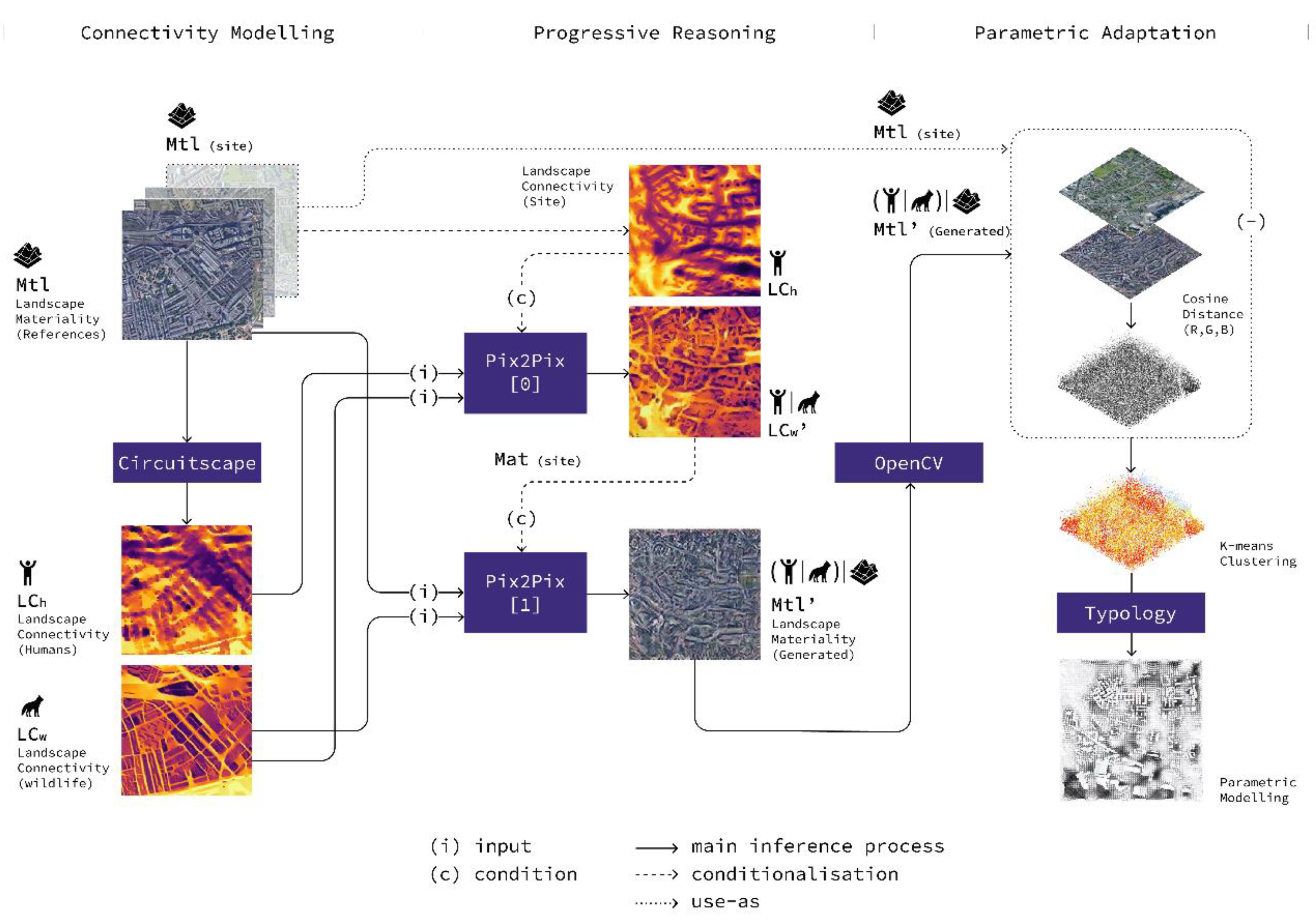
Figure 2.
(a) The current wildlife landscape connectivity (LCw) mapping, and (b) The HOG analysis output of the current connectivity of the site (the coloured area) and the surrounding. A large number of linear features, particularly in the east-west orientation, were detected due to the extensive use of corridors in the area.
Figure 2.
(a) The current wildlife landscape connectivity (LCw) mapping, and (b) The HOG analysis output of the current connectivity of the site (the coloured area) and the surrounding. A large number of linear features, particularly in the east-west orientation, were detected due to the extensive use of corridors in the area.
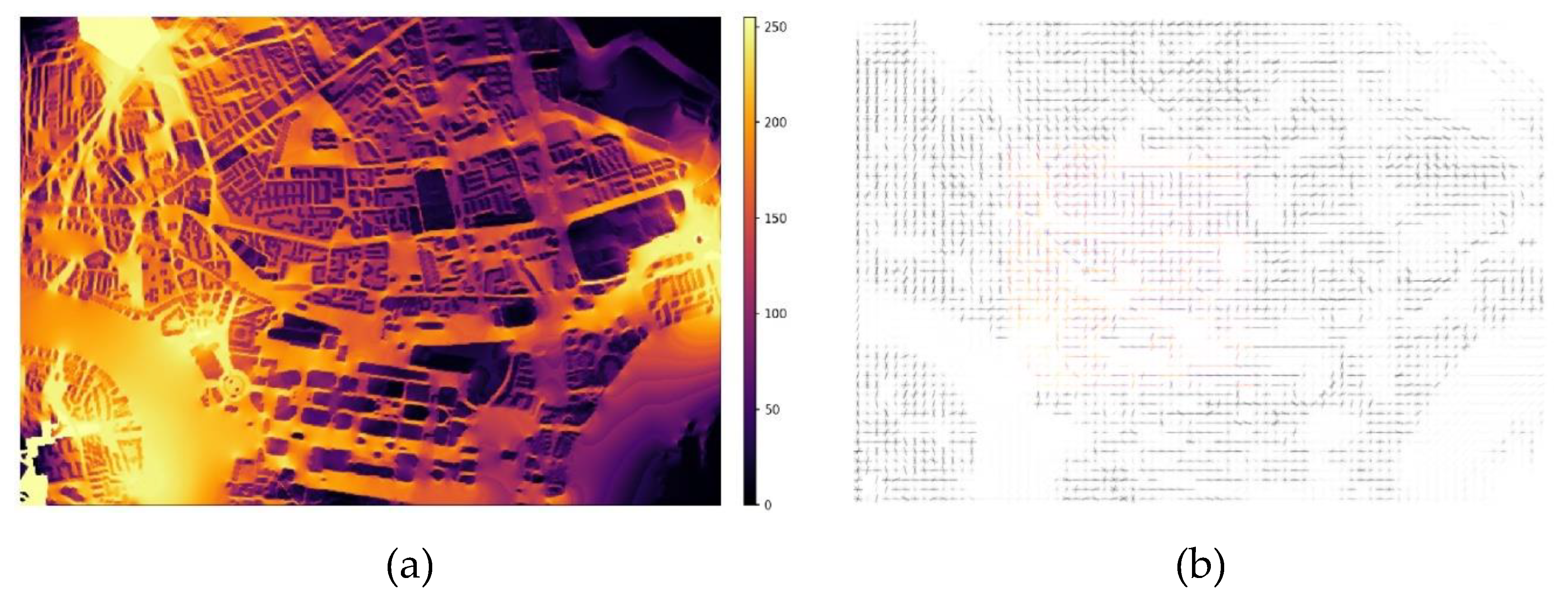
Figure 3.
(a) The overall connectivity (Cm) on wildlife (left half) and human connectivity (right half) datasets, (b)The Kernel Vitality (Vk) on the wildlife data within NBI and eBird datasets, (c) The box plot of NBI and eBird wildlife landscape connectivity (LCw) HOG variance.
Figure 3.
(a) The overall connectivity (Cm) on wildlife (left half) and human connectivity (right half) datasets, (b)The Kernel Vitality (Vk) on the wildlife data within NBI and eBird datasets, (c) The box plot of NBI and eBird wildlife landscape connectivity (LCw) HOG variance.
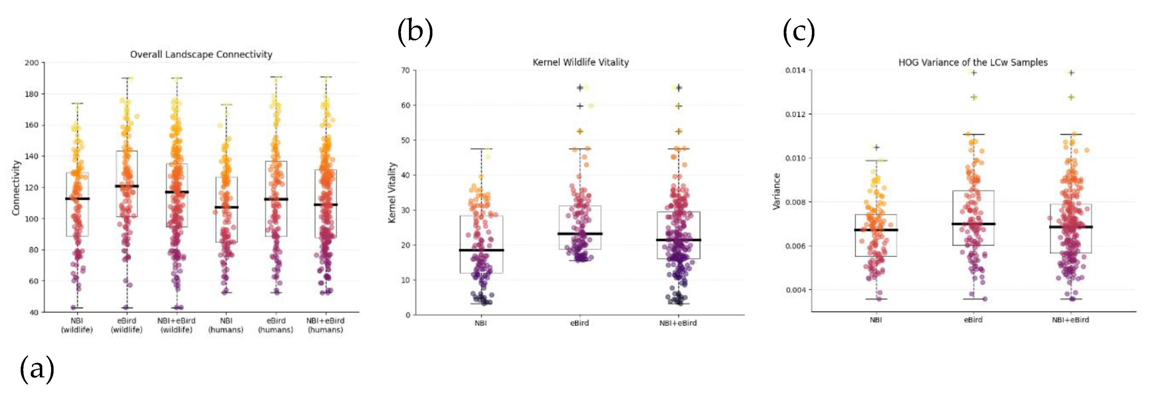
Figure 4.
The presentation of NBI and ebird dataset.
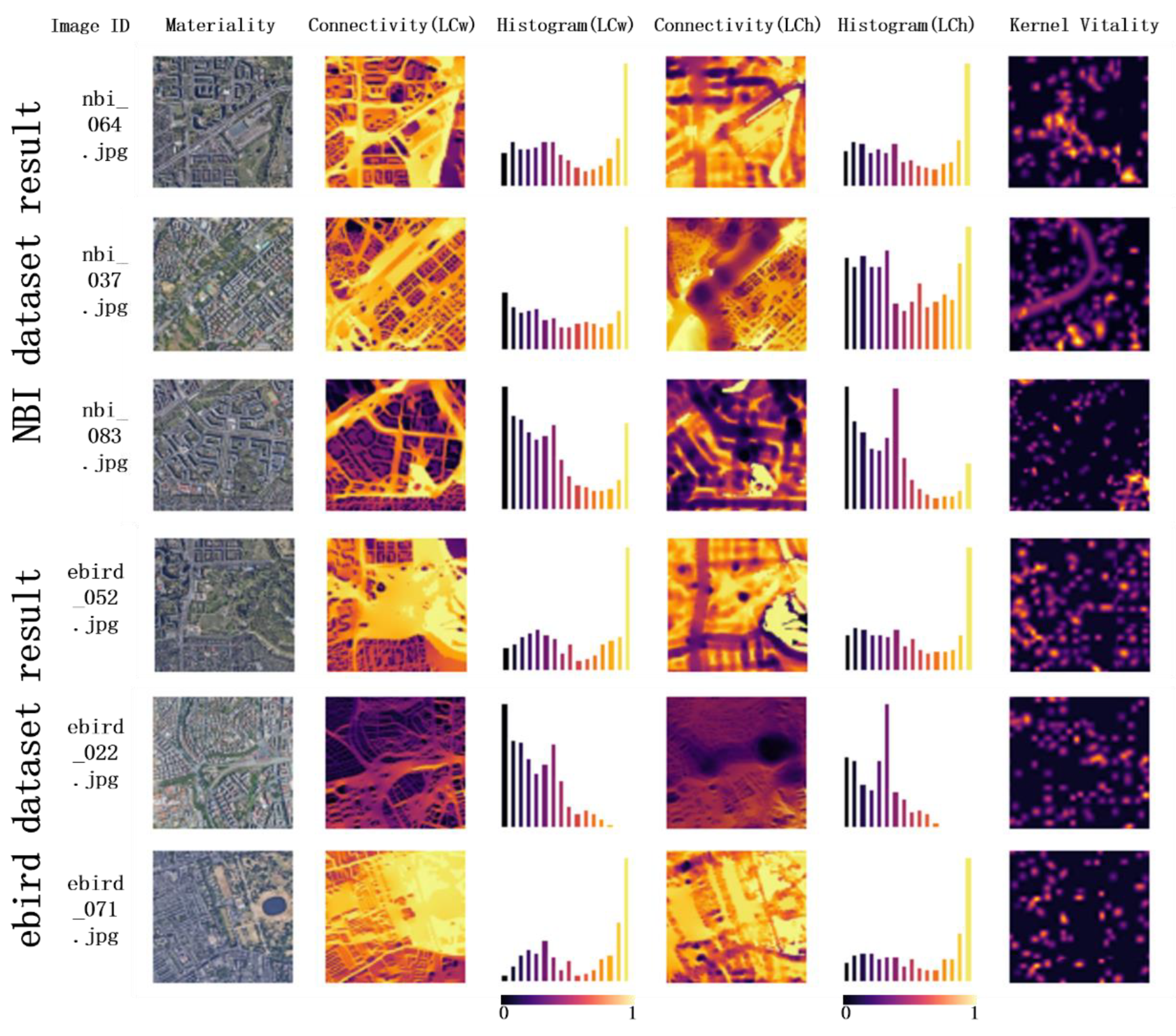
Figure 5.
The workflow of Pix2Pix model.
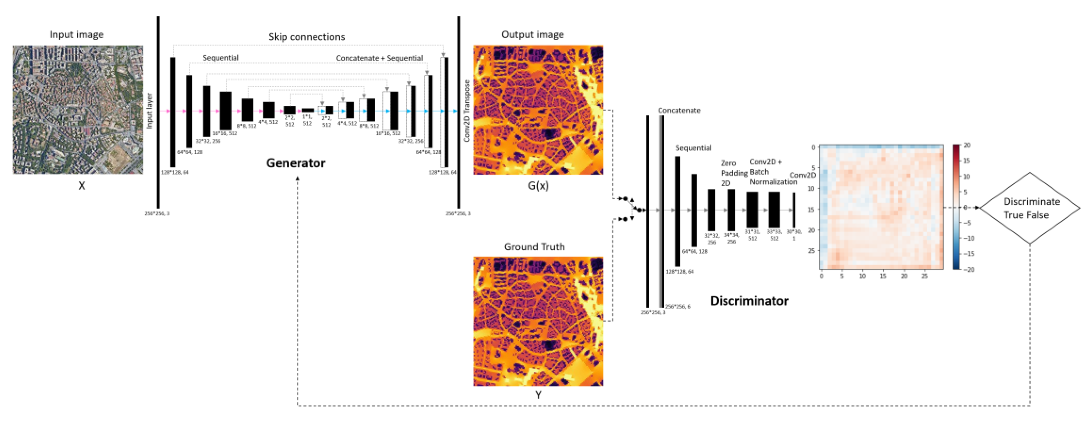
Figure 6.
The two-phase progressive reasoning process that employs two concatenated Pix2Pix models.
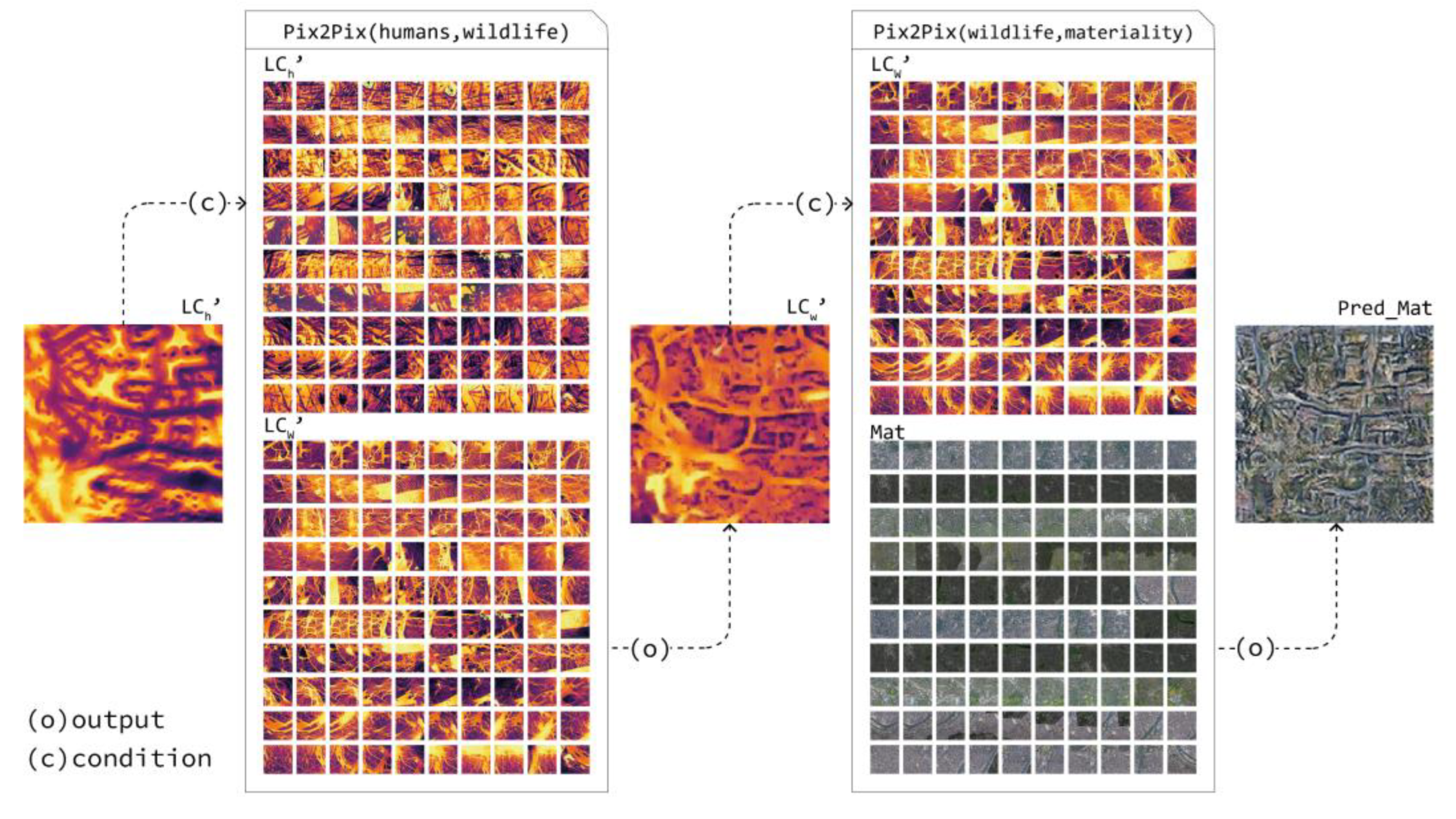
Figure 7.
The suggested design scheme of the trained models and their correlation with surrounding areas: The left column represents landscape connectivity for wildlife, while the right column displays maps illustrating landscape materiality. Horizontally, from top to bottom, are the site’s current condition, outputs from the NBI dataset, and outputs from the eBird dataset.
Figure 7.
The suggested design scheme of the trained models and their correlation with surrounding areas: The left column represents landscape connectivity for wildlife, while the right column displays maps illustrating landscape materiality. Horizontally, from top to bottom, are the site’s current condition, outputs from the NBI dataset, and outputs from the eBird dataset.
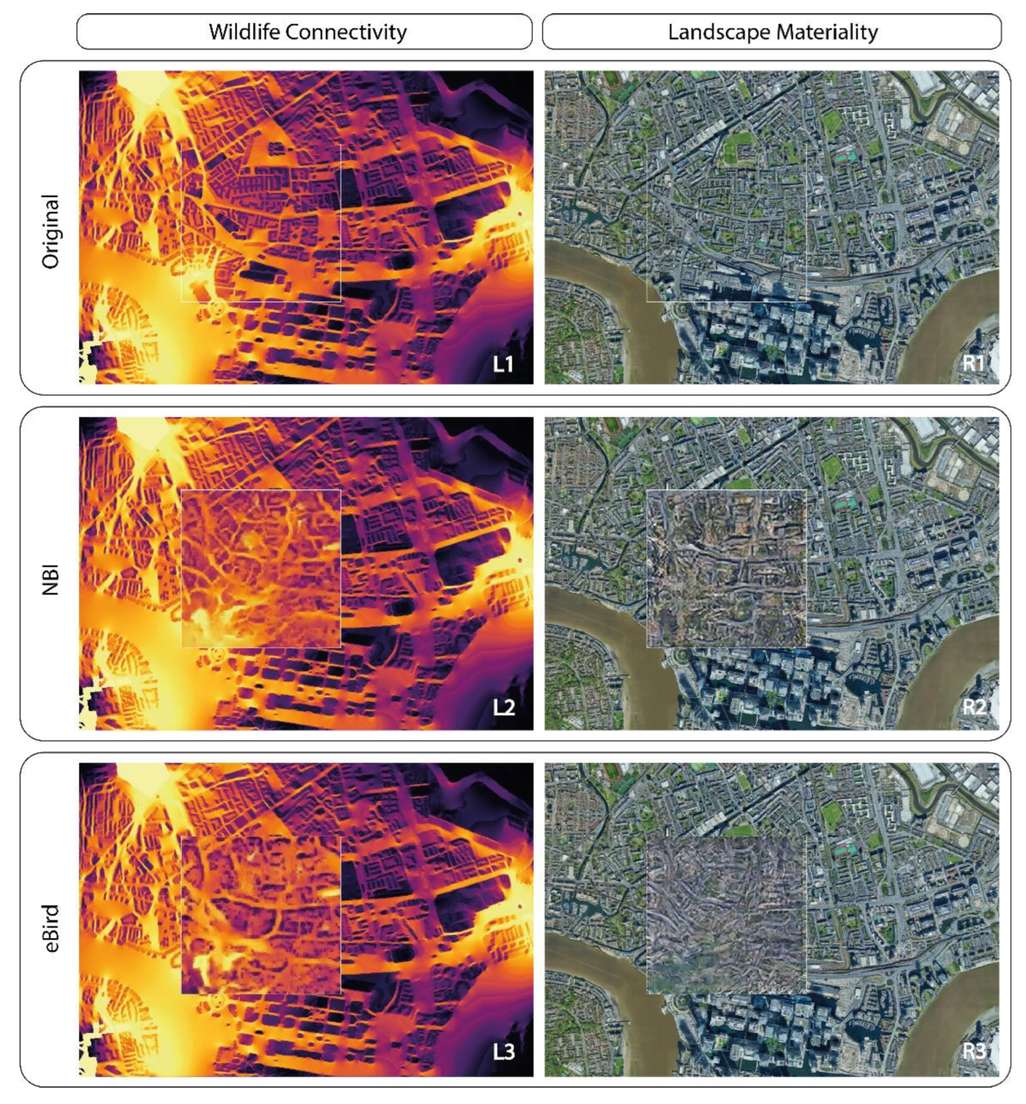
Figure 8.
Measuring the distance between the suggested materiality and the actual materiality of the site.
Figure 8.
Measuring the distance between the suggested materiality and the actual materiality of the site.
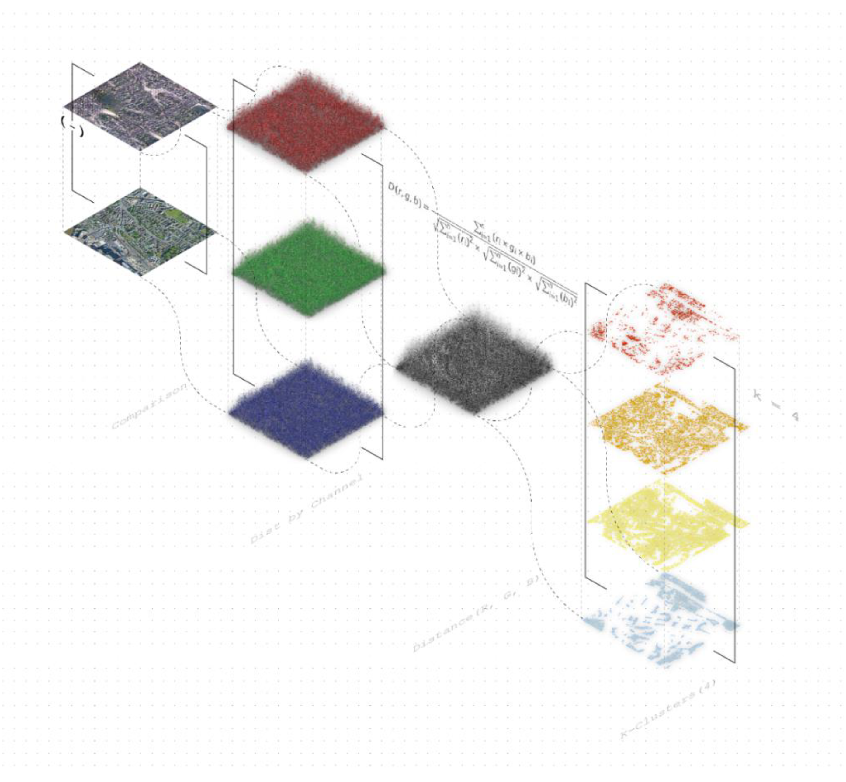
Figure 9.
The linear regression for overall landscape connectivity Cm and HOG variance V is conducted using NBI (top) and eBird (bottom) data. The HOG sampling is performed on images with a resolution of 256x256 pixels.
Figure 9.
The linear regression for overall landscape connectivity Cm and HOG variance V is conducted using NBI (top) and eBird (bottom) data. The HOG sampling is performed on images with a resolution of 256x256 pixels.
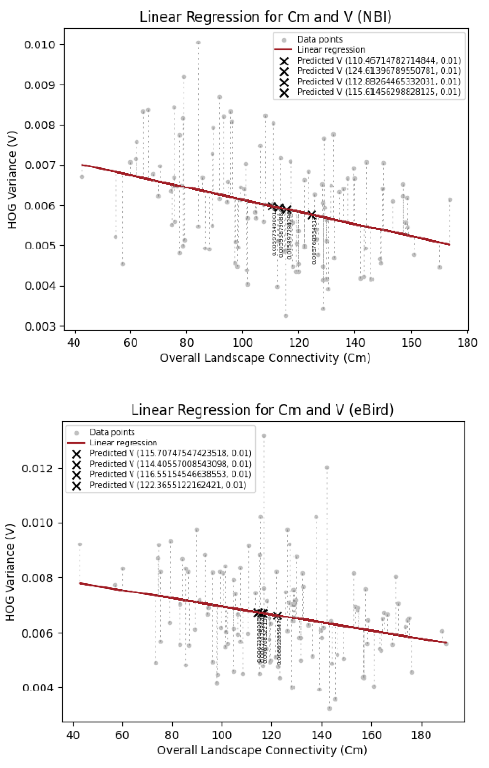
Figure 10.
A listing of all the LCw’ candidates with corresponding Cm values for NBI (upper row) and eBird (lower row) groups. NBI_LCw’_0.png and eBird_LCw’_3.png are selected due to their proximity to their mappings within the ‘good ecological connected landscape’ model.
Figure 10.
A listing of all the LCw’ candidates with corresponding Cm values for NBI (upper row) and eBird (lower row) groups. NBI_LCw’_0.png and eBird_LCw’_3.png are selected due to their proximity to their mappings within the ‘good ecological connected landscape’ model.
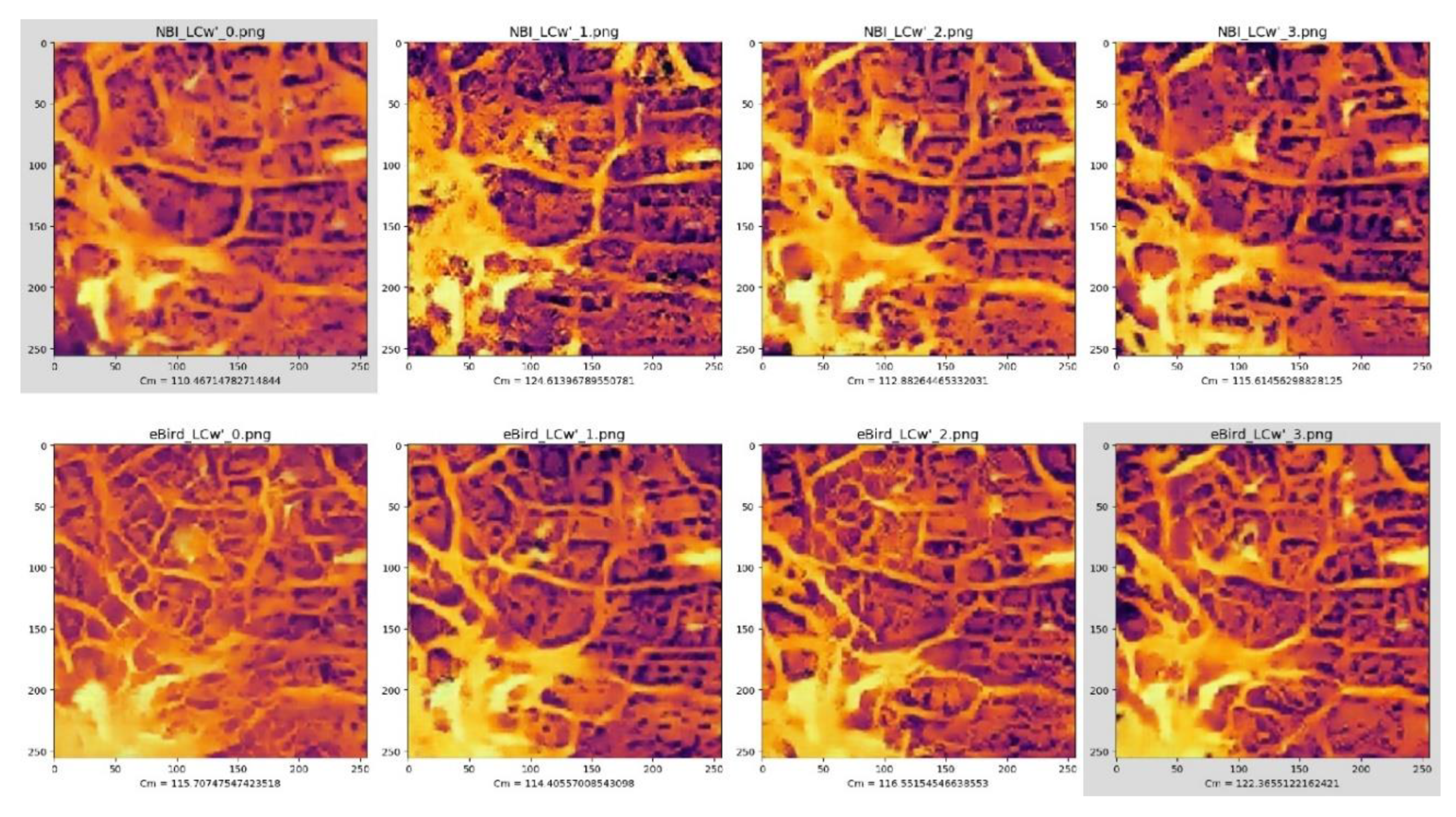
Figure 11.
The LCw’ candidates with corresponding V values for NBI (upper row) and eBird (lower row) groups.
Figure 11.
The LCw’ candidates with corresponding V values for NBI (upper row) and eBird (lower row) groups.
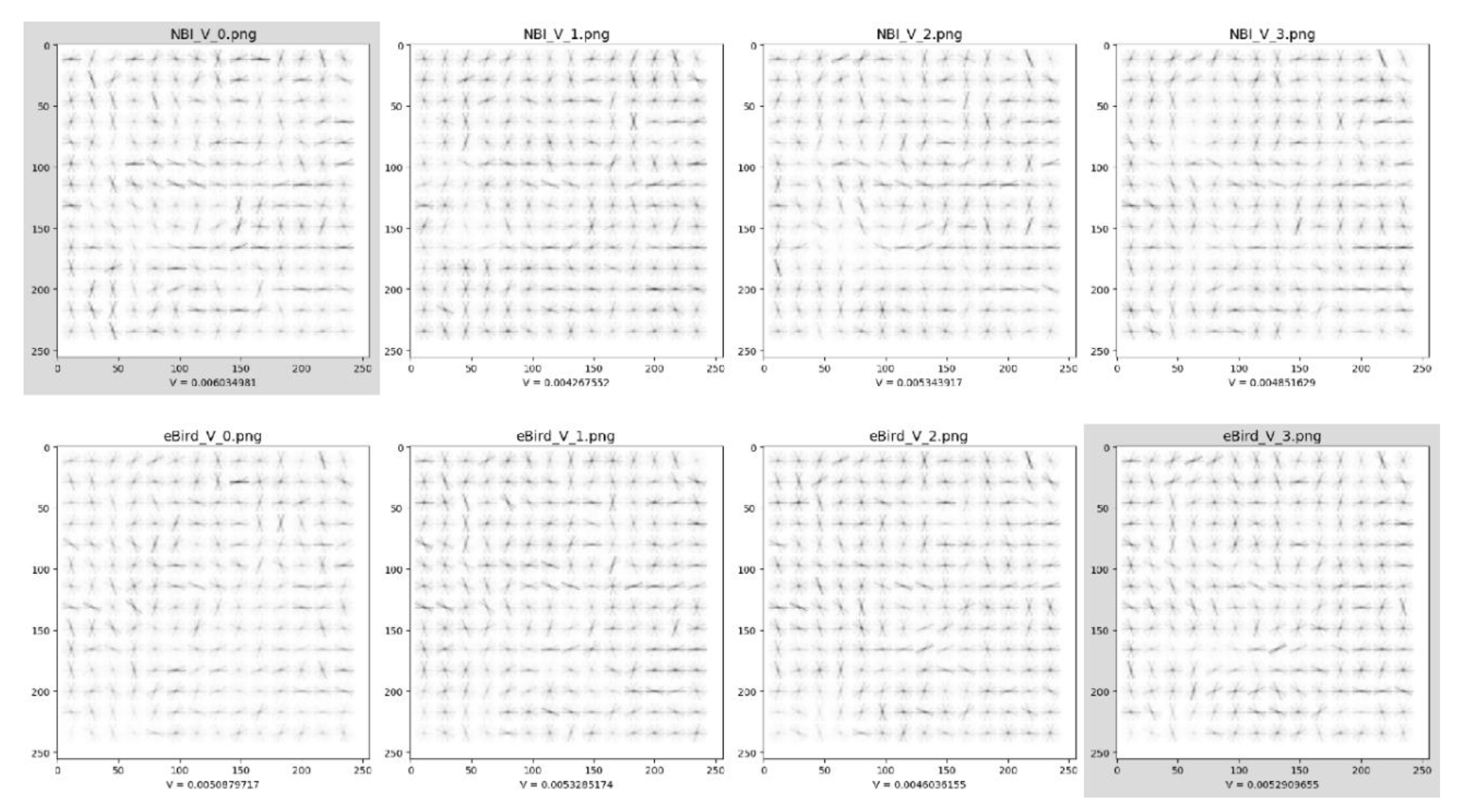
Figure 12.
Joint latent space visualisation for NBI and eBird LCw data. Images with gold borders are from the NBI dataset, while turquoise-bordered ones are from the eBird dataset. The two images marked by red borders represent selected LCw’ maps from both datasets. Central cross-shaped icons denote the centroids of the NBI and eBird populations.
Figure 12.
Joint latent space visualisation for NBI and eBird LCw data. Images with gold borders are from the NBI dataset, while turquoise-bordered ones are from the eBird dataset. The two images marked by red borders represent selected LCw’ maps from both datasets. Central cross-shaped icons denote the centroids of the NBI and eBird populations.
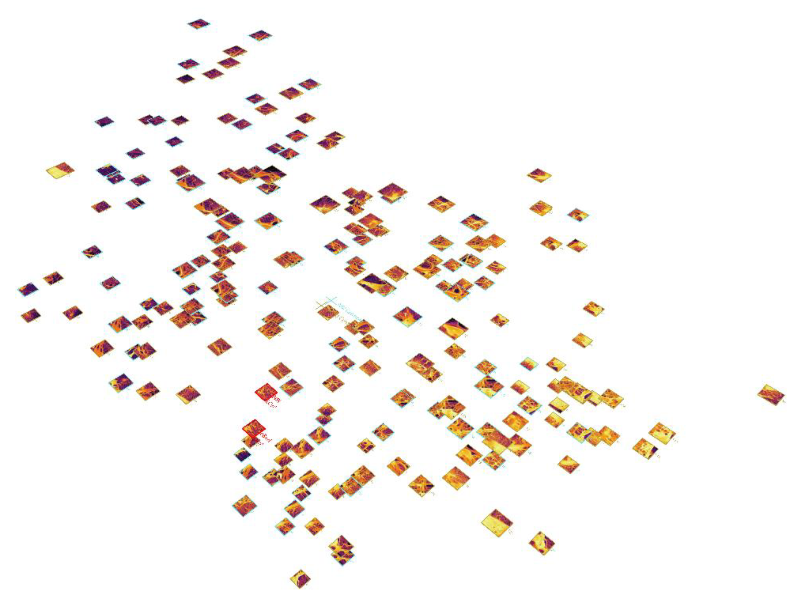
Figure 13.
Visualisation of the joint latent space of NBI and eBird landscape materiality data.
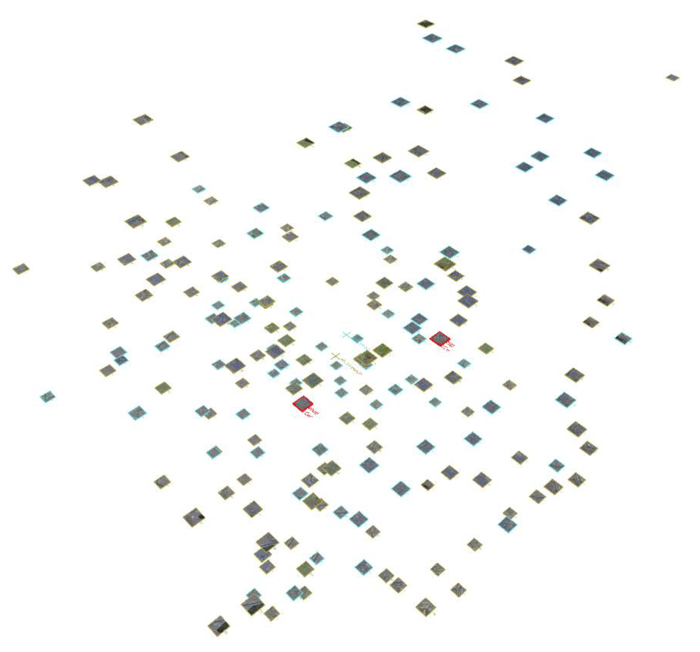
Table 2.
Table for notations.
| Symbol | Implication | |
|---|---|---|
| LCh | Human landscape connectivity | |
| LCh’ | human landscape connectivity of the site | |
| LCw | Wildlife landscape connectivity | |
| LCw’ | wildlife landscape connectivity of the site | |
| Cm | overall connectivity metric | |
| Vk | kernel connectivity vitality |
weight(V) = 0, if V ∈ Vi 1, if V ∈ Ve and 0 < V < 128 1.5, if V ∈ Ve and 128 ≤ V ≤ 255 Vk = (Σweight(V) for all V in grid) / N |
*Notes. Vjk represents the voltage from raster grid node j to k, and Rhjik , Rwjik signifies the effective human resistance and wildlife resistance traversing on landscape material i from raster grid node j to k respectively.
Table 3.
Evaluation upon the datasets.
| Analytical Metrics | NBI dataset | eBird dataset | ||||
| Mean | Maximum | Minimum | Mean | Maximum | Minimum | |
| Overall Landscape Connectivity for wildlife (LCw) | 109.950555 | 173.689041 | 42.838791 | 122.214679 | 190.030716 | 42.838791 |
| Overall Landscape Connectivity for human (LCh) | 106.372746 | 173.587150 | 55.463537 | 114.698759 | 190.012981 | 54.574334 |
| kernel vitality (Vk) | 19.741083 | 47.520000 | 3.150000 | 25.948667 | 65.240000 | 15.460000 |
| Histogram of Oriented Gradients (HOG) | 0.005983 | 0.010055 | 0.003247 | 0.006625 | 0.013190 | 0.003247 |
Table 4.
List of parameters settings of the Pix2Pix models. Two models share the same settings.
| Hyperparameter | Settings |
|---|---|
| Deep Learning Platform | TensorFlow 2.9 and Keras |
| Buffer Size | 400 |
| Batch Size | 1 |
| Image I/O Shape | Width, Depth, Channel = (256, 256, 3) |
| Data Augmentation | Resizing, Random Rotation, Normalisation |
| Generator Optimizer | Adam |
| Discriminator Optimizer | Adam |
| Lambda | 100 |
| Learning rate of Generator | 0.0002 |
| Learning rate of Discriminator | 0.0002 |
| Epoch | 1000 |
Table 5.
The data for and results of calculating the distances between the predicted HOG variance values and the measured HOG variance values, on both NBI and eBird LCw' candidates.
Table 5.
The data for and results of calculating the distances between the predicted HOG variance values and the measured HOG variance values, on both NBI and eBird LCw' candidates.
| LCW' Candidate ID | Predicted HOG Variance | Measured HOG Variance | Distance (Absolute) |
|---|---|---|---|
| NBI_LCw'_0.png | 0.0059754900 | 0.004851629 | 0.0000594910 |
| NBI _LCw'_1.png | 0.0057605545 | 0.005343917 | 0.0014930026 |
| NBI _LCw'_2.png | 0.0059387909 | 0.004267552 | 0.0005948741 |
| NBI _LCw'_3.png | 0.0058972843 | 0.006034981 | 0.0010456553 |
| eBird_LCw'_0.png | 0.0058958727 | 0.0050879717 | 0.0008079010 |
| eBird_LCw'_1.png | 0.0059156528 | 0.0053285174 | 0.0005871354 |
| eBird_LCw'_2.png | 0.0058830485 | 0.0046036155 | 0.0012794330 |
| eBird_LCw'_3.png | 0.0057947158 | 0.0052909655 | 0.0005037503 |
Notes: These values are rounded to the 10th decimal place after the decimal point, employing the method of rounding off to the nearest whole number. NBI_LCw’_0.png and eBird_LCw’_3.png are selected to be the conditional image for the following LCw-materiality reasoning process.
Disclaimer/Publisher’s Note: The statements, opinions and data contained in all publications are solely those of the individual author(s) and contributor(s) and not of MDPI and/or the editor(s). MDPI and/or the editor(s) disclaim responsibility for any injury to people or property resulting from any ideas, methods, instructions or products referred to in the content. |
© 2024 by the authors. Licensee MDPI, Basel, Switzerland. This article is an open access article distributed under the terms and conditions of the Creative Commons Attribution (CC BY) license (http://creativecommons.org/licenses/by/4.0/).
Copyright: This open access article is published under a Creative Commons CC BY 4.0 license, which permit the free download, distribution, and reuse, provided that the author and preprint are cited in any reuse.


