
Submitted:
26 July 2024
Posted:
29 July 2024
You are already at the latest version
Abstract
In this paper, we study nonlocal problems for a fractional diffusion equation and a degenerate hyperbolic equation with singular coefficients in the lower terms. The uniqueness of the solution to the problem is proved by the method of energy integrals. The existence of a solution is equivalently reduced to the question of the solvability of Volterra integral equations of the second kind and a fractional differential equation. For a particular solution of the proposed problem, its visualization is carried out for various values of the order of the fractional derivative. It is shown that the order of the derivative affects the intensity of the diffusion process (subdiffusion), as well as the shape of the wave front.
Keywords:
boundary value problem
; fractional order differential equation
; Gauss hyper-geometric function
; uniqueness of a solution
; existence of a solution
; singular coefficient
; Wright type function
1. Introduction
Fractional partial differential equations can arise in the mathematical modeling of physical media with fractal geometry [1]. Boundary value problems for the fractional order diffusion equation were studied in [2,3,4,5,6]. In [7] a certain family of generalized derived Riemann–Liouville operators of orders and was studied. Applications of this operator are given in [8]. In [9] the unique solvability of the problem for the Riemann–Liouville partial fractional derivative equation with a boundary condition containing a generalized fractional integro-differentiation operator was investigated. The problem in which the boundary condition contains a linear combination of generalized fractional operators with a hyper-geometric Gaussian function for a mixed type equation with the partial fractional Riemann–Liouville derivative was studied in [10]. The nonlocal boundary value problem for a mixed type equation with the Riemann–Liouville fractional partial derivative was studied in [11]. A non-local boundary value problem for Gellerstedt equation with singular coefficient in an unbounded domain was investigated in [12].
The article’s research plan is structured as follows. Section 1 provides information about the problem under study and provides relevant links to articles. Section 2 provides the problem statement. Section 3 provides the main results: the issues of existence and uniqueness of the solution are investigated. Section 4 provides the statement of the proposed problem in a particular case, and Section 5 provides the methodology for solving this problem with its visualization.
2. Formulation of a Problem
In (1) are some real numbers satisfying conditions , .
The equation (1) is considered in domain , where is the half-plane , is the finite region of the fourth quadrant of the plane, limited by the characteristics
equations (1) coming from points , and intersecting at point and the segment of the straight line .
Let’s introduce the notation: is the unit interval of the line , is the intersection point of the characteristic of equation (1) coming from the point with the characteristic .
is a generalized fractional integro-differentiation operator with a hypergeometric Gauss function introduced by M.Saigo [14] and having the form for real and
in particular
Note that if , then the formulas are valid
where and are fractional Riemann–Liouville integration and differentiation operators of the order [13];
Problem A. Find a solution of the equation (1) in domain D satisfying the boundary conditions
and the transmission conditions
Here , are valid constants, are given functions such that
Note that non-local boundary value problems for Equation (1) in unbounded and bounded domains are studied in [15,16].
We will look for a solution to the problem in the class of doubly differentiable functions in domain of D such that
3. Main Results
3.1. Uniqueness of the Solution of the Problem
Theorem 1.
Let , Then problem A, has only a trivial solution.
Proof of Theorem 1.
Let’s introduce the following notation
It is known [17] that the solution of equation (1) in domain satisfies the condition (6) and the condition
is given by the formula
where is a Wright type function [17].
It is also known [18] that the functional relation between and , brought from the parabolic part of to the line , has the form
Let’s find the ratio between and brought to the line from the hyperbolic part of domain D.
Substituting into the boundary condition (7) and applying successively the relations [14]
after simple calculations, we get
where
Applying the operator to both parts of the resulting equality, taking into account (18), (3), (4) and we have
where
Consider the corresponding homogeneous problem:
Consider the following two cases:
where
Let’s evaluate the following integral
and therefore, by virtue of ratio (15) we have
Hence, due to the conditions (10), we obtain an estimate in domain of for the integral:
Now let’s find the estimate of the integral I in domain .
For , the equality (22) takes the form
and therefore,
Next, let’s use the well-known formula for the gamma function [19]
Assuming to it, we get
Applying this formula and the Dirichlet formula of the permutation of the order of integration in the repeated integral, we arrive at the relation
From the conditions of the theorem we obtain
Hence, by virtue of the conditions (10) and the equalities we get
b) Let :
Then (20) is a homogeneous Abel equation:
having only a trivial solution .
3.2. The Existence of a Solution to Problem A
Theorem 2.
Let a) b) c) d) Then there is a solution to problem A.
Proof of Theorem 2.
According to (14) and (15), to prove the existence of a solution to problem A, it is enough to find .
Consider the case then (29) gives an explicit expression for that is, and are found by the formula (15).
If then (29) is an Abel integral equation of the first kind.
with According to the condition (10) Function is also continuous [10] and the well-known solution of the equation (30)[13] gives an explicit expression for in the form
If then the equation (29) takes the form
As you know [13] if
then the formula is correct
where
If the condition (33) is satisfied, then applying the operator to both parts of (32) and considering (34) we arrive at the integral equation:
where
4. Formulation of a Problem
Let , , then the equation (1) takes the form
In this case, let’s study the following problem.
Problem B. Find a solution of equation (40) satisfying the boundary condition (6) and the condition
and the transmission conditions
Here is given function such that
5. Solution Methodology
Solving a modified Cauchy problem with initial data
in domain for equation is given by the d’Alembert’s formula
From (44) we calculate
Substituting into the condition (41), we obtain the second functional relation between the unknown functions and
Applying the method of variation of constants to the equation (46), we will have
where constant values.
Given that , from (47) it is easy to show that
Using the found and , it is easy to obtain a solution to problem B in each of the areas and , which means that the solution to the problem (40), (6), (41) in a given class of functions in the domain D, satisfying the boundary conditions (6), (41) and the gluing conditions (42)-(43).
Let’s consider an example of solving problem B for a specific type of function with its visualization. Visualization was performed using PyCharm software in the Python language.
Example 1.
Let .
Then equalities (47), (5) take the following form
where
Here is the modified Bessel function, is the gamma function, is the beta function.
Figure 1 shows the graphs of functions and for and .
Using the obtained functions and , we can obtain a solution to the problem in domain and , respectively, using formulas (14) and (42).
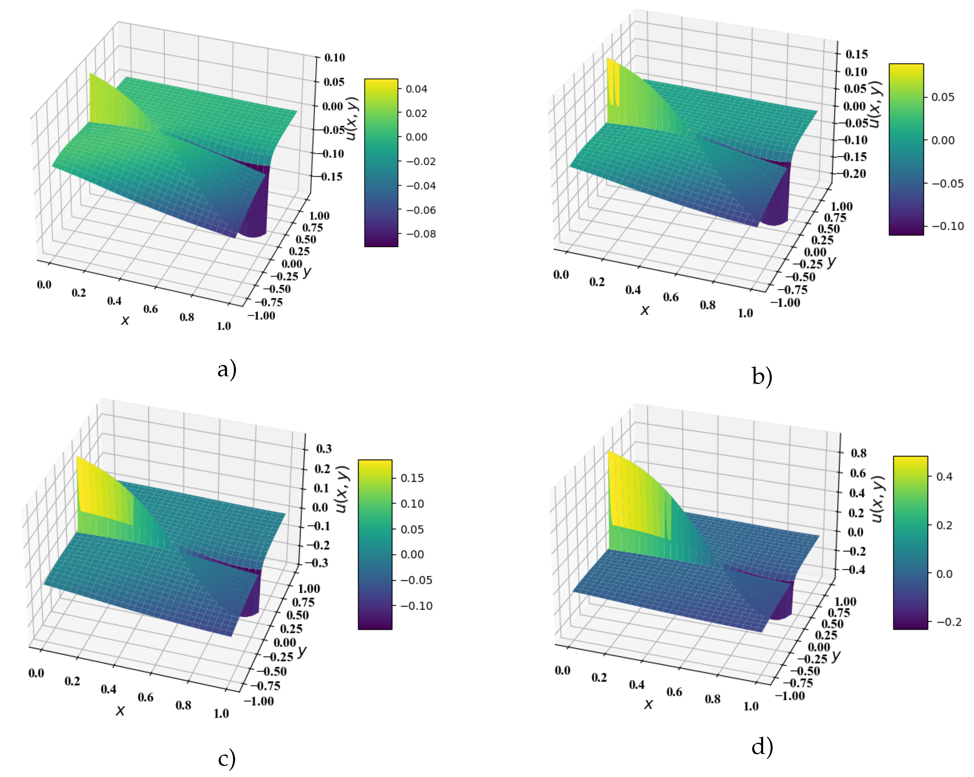
Let us present graphs of the solution of Problem B using formulas (14) and (42) depending on the values of parameter .
In Figure 2 we can see that when changing the parameter in domain the subdiffusion mode is enhanced due to the fact that the diffusion process proceeds more slowly than normal diffusion. We see that the region of positive values of the solution function expands, and the region of negative values, on the contrary, narrows. In domain the wave mode proceeds, the shape of which is also affected by the values of parameter .
6. Discussion
The properties of solution of Equation (1) at essentially depend on coefficients and , at the lowest terms of Equation (1). If , then the solution to Equation (1) on the parabolic degeneracy line has a logarithmic singularity. In this case boundary value problems for Equation (1) at are studied with different conditions.
7. Conclusions
In this work, we study a boundary value problems for differential equation with partial fractional derivative and degenerate hyperbolic equation. Main results are new. Using these results, we can explore various boundary value problems for differential equations with partial fractional derivative of the second and higher orders.
The paper provides an example of solving a non-local problem in a particular case, and plots the functions. It is shown that the order of the fractional derivative affects the intensity of diffusion, it slows down, which corresponds to subdiffusion. Also, the order of the fractional derivative affects the shape of the wave front.
Author Contributions
Conceptualization, M.R., R.P., R.Z. and N.Y.; methodology, M.R., R.P., R.Z. and N.Y.; validation, M.R., R.P., R.Z. and N.Y.; investigation, M.R., R.P., R.Z. and N.Y.; writing—original draft preparation, M.R., R.P., R.Z. and N.Y.; writing—review and editing, M.R., R.P., R.Z. and N.Y.; supervision, M.R. and R.P. All authors have read and agreed to the published version of the manuscript.
Funding
Agreement between the V.I. Romanovsky Institute of Mathematics of the Academy of Sciences of the Republic of Uzbekistan and the Federal State Budgetary Scientific Institution Institute of Cosmophysical Research and Radio Wave Propagation of the Far Eastern Branch of the Russian Academy of Sciences on cooperation in the field of mathematical research (no 117, April 28, 2022).
Institutional Review Board Statement
Not applicable
Data Availability Statement
Not applicable.
Acknowledgments
Authors would like to thank anonymous referees.
Conflicts of Interest
The authors declare no conflicts of interest.
References
- Nakhushev, A.M. Elements of fractional calculus and their application.; Publishing House of the KBSC RAS: Nalchik, Russia, 2000. [Google Scholar]
- Gekkieva, S.Kh. On one analogue of the Tricomi problem for a mixed-type equation with a fractional derivative. Reports of AMAN 2001, 5(2), 18–22. [Google Scholar]
- Gekkieva, S.Kh. The Cauchy problem for the generalized transport equation with a fractional derivative in time. Reports of AMAN 2000, 5(1), 16–19. [Google Scholar]
- Kilbas, A.A.; Repin, O.A. An analogue of the Bitsadze–Samarsky problem for a mixed-type equation with a fractional derivative. Diff. equations 2003, 39(5), 638–644. [Google Scholar]
- Pskhu, A.V. Solution of boundary value problems for the fractional order diffusion equation by the Green’s function method. Diff. equations 2003, 39(10), 1430–1433. [Google Scholar]
- Pskhu, A.V. Solution of the boundary value problem for partial differential equations of fractional order. Diff. equations 2003, 39(10), 1092–1099. [Google Scholar]
- Tomovski, Z.; Hilfer, R.; Srivastava, H.M. Fractional and operational calculus with generalized fractional derivative operators and Mittag-Leffler type functions. Integ. Trans. and Special functions. 2010, 21(11), 797–814. [Google Scholar] [CrossRef]
- Hilfer, R. Experimental evidence for fractional time evolution in glass forming materials. Chemical Phys 2002, 1-2, 399–408. [Google Scholar] [CrossRef]
- Tarasenko, A.V.; Egorova, I.P. On a non-local problem with a fractional Riemann–Liouville derivative for a mixed type equation. Bulletin of the Sam.state Technical University. Ser. phys.-mat of Science 2017, 21, 112–121. [Google Scholar]
- Repin, O.A. On a problem for a mixed type equation with a fractional derivative. Izves. Vuz. Matem. 2018, 8, 46–51. [Google Scholar] [CrossRef]
- Ruziev, M. Kh; Yuldasheva, N.T. Nonlocal boundary value problem for a mixed type equation with fractional partial derivative. Journal of Mathematical Sciences 2023, 274, 275–284. [Google Scholar] [CrossRef]
- Ruziev, M.K.; Yuldasheva, N.T. On a boundary value problem for a class of equations of mixed type. Lobachevskii Journal of Mathematics 2023, 44, 2916–2929. [Google Scholar] [CrossRef]
- Samko, S.G.; Kilbas, A.A.; Marichev, O.I. Integrals and derivatives of fractional order and some of their applications; Science and Technology: Minsk, Belarus, 1987; pp. 154–196. [Google Scholar]
- Saigo, M. A remark on integral operators involving the Gauss hypergeometric function. Math. Rep. Coll. Gen.Educ.Kyushe Univ. 1978, 11(2), 135–143. [Google Scholar]
- Ruziev, M. Kh. A boundary value problem for a partial differential equation with fractional derivative. Fractional calculus and Applied Analysis. 2021, 24(2), 509–517. [Google Scholar] [CrossRef]
- Ruziev, M.K.; Zunnunov, R.T. On a nonlocal problem for mixed type equation with partial Riemann–Liouville fractional derivative. Fractal and Fractional 2022, 6, 110. [Google Scholar] [CrossRef]
- Pskhu, A.V. Partial differential equations of fractional order. Nauka: Moscow, 2005; 199 p.
- Gekkieva, S.K. An analogue of the Tricomi problem for a mixed type equation with a fractional derivative. Izv. Kabardino-Balkarian Scientific Center of the Russian Academy of Sciences 2001, 2, 78–80. [Google Scholar]
- Prudnikov, A.P.; Brychkov, Yu.A.; Marichev, O.I. Integrals and series. Elementary functions. Nauka: Moscow, Russia, 1981; pp. 800.
- Kilbas, A.A. Integral equations: a course of lectures. BSU: Minsk, Belarus, 2005; 143 p.
Figure 1.
Graphs of functions for : a) ; b) .
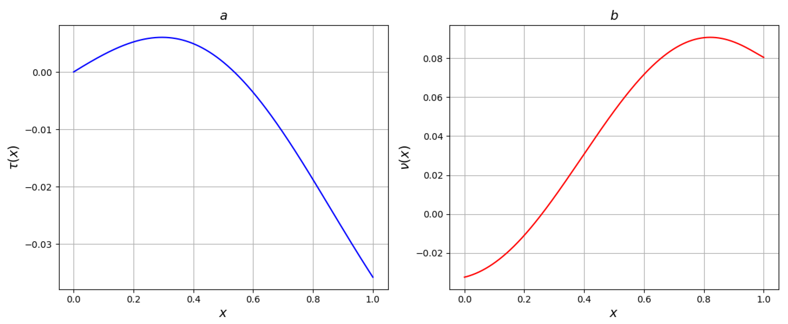
Figure 2.
Graphs of the solution of Problem B for and different values of : a) ; b) ; c) ; d) .
Disclaimer/Publisher’s Note: The statements, opinions and data contained in all publications are solely those of the individual author(s) and contributor(s) and not of MDPI and/or the editor(s). MDPI and/or the editor(s) disclaim responsibility for any injury to people or property resulting from any ideas, methods, instructions or products referred to in the content. |
© 2024 by the authors. Licensee MDPI, Basel, Switzerland. This article is an open access article distributed under the terms and conditions of the Creative Commons Attribution (CC BY) license (http://creativecommons.org/licenses/by/4.0/).
Copyright: This open access article is published under a Creative Commons CC BY 4.0 license, which permit the free download, distribution, and reuse, provided that the author and preprint are cited in any reuse.


