Submitted:
26 July 2024
Posted:
27 July 2024
You are already at the latest version
Abstract
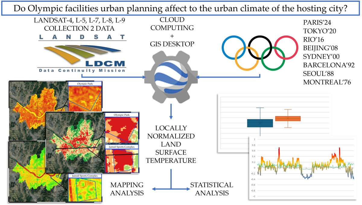
The Olympic Games are a sporting event and a catalyst for urban development in the host city. In this study, we utilized remote sensing and GIS techniques to examine the impact of the Olympic infrastructure on the surface temperature of urban areas. Using Landsat Series Collection 2 Tier 1 Level 2 data, cloud computing, and Google Earth Engine (GEE) methods, this study examines the effects of various Olympic Games facility urban planning in different historical moments and location typologies: monocentric, polycentric, peripheric and clustered Olympic ring. The GEE code applies to the Olympic Games from Paris’24 to Munich’72. However, this paper focuses specifically on the representative cases of Paris’24, Tokyo’20, Rio’16, Beijing’08, Sydney’00, Barcelona’92, Seoul’88, and Montreal’76. The study is not only concerned with obtaining absolute Land Surface Temperatures (LST), but rather the relative influence of mega-event infrastructures on mitigating or increasing the urban heat. As such, locally Normalized Land Surface Temperature (NLST) was utilized for this purpose. In some cities (Paris, Tokyo, Beijing, and Barcelona), it is identified that Olympic planning has resulted in the development of green spaces, creating "green spots" that contribute to lower-than-average temperatures. However, it should be noted that there is a significant variation in temperature within intensely built-up areas, such as Olympic villages and the surrounding areas of the Olympic stadium, which can become “hotspots”. Therefore, it is important to acknowledge that different planning typologies of Olympic infrastructure can have varying impacts on city heat islands, with the polycentric and clustered Olympic ring typologies displaying a mitigating effect. This research contributes to a cloud computing method that can be updated for future Olympic Games or adapted for other mega-events and utilizes a widely available remote sensing data source to study a specific urban planning context.
Keywords:
Normalized land surface temperature
; cloud computing
; surface urban heat island
1. Introduction
Mega-events such as Olympic Games, may significantly transform the urban landscape of the host cities [1,2,3,4,5]. The urban planning process driven by the Olympic event can lead to an increase or mitigation of urban surface temperatures, suggesting that the design of Olympic facility locations and structures can impact the urban climate. Considering the future challenges posed by climate change, this study focuses on analysing the impact of Olympic facilities on the Surface Urban Heat Island (SUHI) effect, which is nested using Land Surface Temperature (LST) remote sensing data.
1.1 Olympic Games Urban Planning
Over time, mega-events have induced major urban transformations [6,7,8,9,10]. As observed in the following section, the Summer Olympic Games were developed through a model of sports promotion that transformed into a model of metropolitan development [11]. To analyse the different main stages of urban transformation in the host cities, we will examine the evolution through five different phases [3].
Phase I: Minimal Transformation (1896–1924):
The first phase of the Olympic Games began with the event’s first edition, until the construction of the first Olympic Village in Paris in 1924. Throughout this phase, sub-sequent editions were characterized by private funding, an interest in promoting sports through host cities, and economic organization. Consequently, Olympic cities in this phase focused on minimal transformations, proposing models of temporary accommodation in military areas or through public availability [4].
Phase II: Emerging Spatial Organisation (1932–1956):
In the second phase, the Olympic cities will focus on the construction of sports facilities for the foundation of a new sports district in the peripheral areas of the cities. The Olympic editions in the second phase catalyzed the construction of new sports facilities and Olympic accommodations that, in the post-Olympic period, became new permanent neighborhoods for the host cities. Thus, the second phase saw the emergence of spatial organisation and the creation of new practices for infrastructural transformations, which we will observe in the third phase. In this phase, the Berlin 1936 project promoted a new spatial solution for the future host cities of Helsinki and Melbourne [3,4].
Phase III: Reconfiguration of Cities (1960–1988):
In the third phase, the Olympic cities will be deeply inspired by the design of the 1960 Rome Olympic Games. The Rome edition is recognised as the first to consider the Olympic event as an instrument of urban development and as an opportunity for reconfiguring the city [12]. The city of Rome concentrated on working in different areas, developing a modern transport system, and constructing the airport. The 1964 Tokyo edition followed the same philosophy as the previous edition, using the Olympic event as an instrument of urban renewal. However, Tokyo took advantage of the event to promote a ten-year development plan that included improving the infrastructure system, roads, harbour, housing, water supply and public health. The Tokyo edition was one of the Olympics’ most extensive urban development projects [3]. For the 1968 Mexico City edition, a spatial organisation was planned that included the development of new infrastructure and housing to expand a peripheral area of the metropolis. Meanwhile, the Munich 1972 edition proposed redeveloping a brownfield site to construct a sports park, including residences. The Munich plan foresaw the construction of a new self-sufficient community and other road improvements in the city. Various improvements such as the restoration and pedestrianisation of the old town, the expansion of public transport lines, the creation of underground car parks, the development of a new shopping centre and the construction of three new motorways were carried out. Subsequently, the Montreal 1976 and Moscow 1980 editions will propose new housing solutions and infrastructural works to reconfigure the cities. The Montreal’76 edition is recognised as one of the moments of most significant concern for the increase in the size of the Olympic event. The 1984 Los Angeles Games was organised through private funding with existing or temporary structures. On the other hand, the 1988 edition in Seoul allowed the Olympic Games to resume their role as a vehicle for urban transformation. The Seoul project was based on a twenty-year plan that introduced new programmes to ensure higher health and hygiene standards throughout the city. In addition, the project included measures for air pollution, rubbish control, and water quality, as well as a significant plan to decontaminate the Han River. Thanks to the Olympics, the city was able to develop three new underground lines to ease traffic congestion and 47 bus lines were extended. The airport was expanded, and new projects were developed to emphasise the cultural aspects of the Olympic event. The city was able to have a programme of renovation and reconstruction of historical monuments, such as palaces and shrines [3].
Phase IV: Large-Scale Urban Transformations (1992–2004):
The fourth phase begins with Barcelona 1992 (recognised as the best example of the role of the Olympic Games as a catalyst for change and urban renewal) and ended with Athens 2004. Barcelona 1992 proposed a new strategy for reconstructing and redefining post-industrial cities. The transformation of a city in crisis was the common element of all the Olympic cities in this phase. The city of Barcelona has become an example of post-industrial reconversion by constructing a new image for the exploitation of tourism in the post-Olympic period. Thus, the Olympic Games became a means of ensuring a significant change in urban infrastructures through a mixed economy. From 1992 onwards, tourism became a fundamental element of the economy of the host cities in the post-Olympic phase [13]. Barcelona presented a new image and development strategy, inspiring the next candidate cities [14]. Following the same philosophy as Barcelona, Sydney, in 2000, proposed an ambitious project for reconfiguring abandoned areas by applying new sustainable practices. Sydney was recognised as the first Olympic city to introduce the theme of environmental sustainability into the development of the Olympic event 3]. The stadium and Olympic Village, located in the peripheral area of the city, were included in the Homebush Bay area. The area was neglected for many years, and thanks to the Olympia bid, the municipality strengthened and accelerated the renovation of the whole area, establishing a new structural plan for reconfiguring the area [3]. Subsequently, the Athens project in 2004 was included in a programme of transformation of the primary infrastructure of the Greek city. The port’s reconfiguration, the central areas’ redevelopment, the construction of a new airport and the provision of the subway were the major infrastructural works that were advanced for the modernisation of Athens [15].
Phase V: Metropolitan Development (2008–2028):
Finally, the fifth and final phase begins with the first Chinese edition of Beijing 2008 and ends with the last edition assigned to Brisbane in 2032. In this phase, the cities are characterised by metropolitan development that uses the central empty spaces to reconfigure the host cities. Thus, the Olympic Games will emphasise environmental protection and the sustainable development of the Olympic project [2]. The establishment of an environmental park in Beijing [16] or planning a water recycling system in London can be considered an innovative measure for environmental protection in the candidate cities. Furthermore, since London 2012, the tangible and intangible Olympic legacy has assumed great importance for post-Olympic planning [17]. Temporary facilities and innovative solutions are used in the following editions. Compared to previous phases, the Beijing and London projects have favoured the emergence of one-off infrastructure works such as airport reconfiguration and rail and metro expansion [18]. Subsequently, the 2016 edition of Rio de Janeiro brought further changes to the allocation of host cities, which, for the first time, were chosen without any competition. The allocation of the event through a proclamation process involved the inclusion of temporary structures and the reuse of existing sports facilities in the candidate cities. Therefore, the International Olympic Committee (IOC) identified Los Angeles and Brisbane as cities that could represent the new evolution and organisation of the Olympic event. The following stages allow us to affirm that the Olympic Games throughout urban history were inspirational for the candidate cities and that the variables specific to each city have favoured legitimising the Olympic city as a distinct urban genre. Over time, urban planners have proposed different projects that have become development models for other cities. The former stages help us reflect on the history of the physical impact of the Games and how it has changed over the past two centuries [2], but also to contextualise its impact in the surface city heat island.
1.2. Land Surface Temperature (LST) and Surface Urban Heat Island (SUHI)
The evolution of the Land Surface Temperature (LST) can be mapped using thermal satellite sensors that receive the thermal radiance emitted by the Earth’s surface. The land temperature in urbanized spaces is higher than in naturalized spaces due to a greater presence of structures such as buildings, roads and other infrastructure that absorb and re-emit the sun’s radiation more than natural landscapes such as forests and water bodies [19,20]. This phenomenon of urban climate alteration related with the increase in temperatures is known as Urban Heat Island (UHI). An UHI is characterized by differences in ambient temperatures between urban and rural areas. If, instead of analysing atmospheric temperatures for study, satellite images are used to obtain the LST, the concept varies towards a Surface Urban Heat Island (SUHI) [21].
In recent decades, this phenomenon has intensified due to climate change, increasing the frequency and duration of heat waves and driving a thermal increase in urban areas [22]. Consequently, the attenuation of urban temperatures and the mitigation of the impacts of heat waves have been incorporated into the political agendas of cities as measures to increase thermal comfort in those urban populations sensitive to extreme heat.
According to several studies, the conditions that contribute to the creation and intensification of heat islands include the urban structure, materials with low albedo, environmental pollution, and the composition of land uses and covers [23,24,25]. In relation to the latter, several authors highlight the nature and evolution of land uses as key determinants in the surface behaviour of temperatures and pointing out the fundamental role of those covers related to urban green spaces [26,27,28] and their spatial structure to reverse high temperatures through the effects of evapotranspiration or shading generation [29,30,31,32,33,34].
Studies related on the spatial characterization of temperatures show it is not only necessary to focus on dense cities, but also on those peri-urban spaces determined by a daily floating population such as the case of some Olympic Game zones or university campus, which have received less attention with some exceptions [35,36,37,38,39]. Along these lines, recent studies focus on the thermal factor, related to the geographical, landscape and morphological characteristics of Olympic Game infrastructures, where green areas and urbanized areas converge, giving rise to peculiar mixed urbanized and natural landscape configurations [4]. More specifically, recent studies analyse, using thermal satellite images, the spatiotemporal evolution of surface temperature and its relationship with land covers and uses. From the Olympic Games point of view, it is specifically studied for single cities (e.g. Beijing 2008 Summer games by Cai et al [40] and Pyeongchang Winter games [41]), and recently by Tu et al in a wider focus [42].
The main tools for the direct measurement of the urban temperature are evidently based on thermal sensors, either in terrestrial meteorological stations for measuring air temperature, or sensors on board aircraft or satellites for measuring LST. Developed territories usually have networks of meteorological stations equipped with thermometers [43,44], from which spatially specific data are obtained. The advantages of field observations are their proximity to the Earth’s surface and the temporal resolution of the data (e.g. hourly records), but the disadvantage is that they are punctual observations from a geographical point of view, often far from the location of interest to analyse. On the other hand, since the beginning of satellite remote sensing for meteorological purposes in the 1970s (e.g. Meteosat), thermal data of the LST measured from space have been available [45]. The main advantages of satellite observations are the systematic sampling of the territory (global coverage) and the periodicity of measurements. It should be noted, as the main drawbacks of meteorological satellite remote sensing with respect to stations on the ground, aspects such as the need to apply atmospheric corrections and the presence of clouds that can hinder measurements. Despite their drawbacks, satellite remote sensing techniques with thermal sensors have been crucial in the study and monitoring of temperatures from the applied perspective of large agencies [46]. Given the availability of thermal data from satellite missions such as MODIS (already completed) and Landsat (active since the 1970s), their images have been the material and methodological basis of many studies on the spatial behaviour of temperatures at a scientific level [47,48,49,50], with special usefulness in places with a low density of terrestrial meteorological stations [51,52]. Particularly interesting due to their characteristics are the thermal images of the Landsat series of satellites [53], which are obtained every 16 days due to the orbit that the satellite follows and have a spatial resolution of 120 m to 60 m (depending on the sensor), which can be improved to 30 m with techniques such as pan-sharpening from lower resolution bands [54,55]. With them, it is possible to obtain a systematic sampling of the LST continued over time and on a sufficiently detailed scale to analyse the urban surface temperatures, as has been carried out in numerous previous studies throughout the world [56,57,58]. Heat maps from satellites can be used to monitor LST, while optical data collected by satellites can report where and when land use and land cover have changed over time. Once land covers and surface temperatures have been mapped, incorporating socioeconomic data related to population, demographics, and health information into heat vulnerability indices can help guide interventions to manage risks for public health related to heat, as well as the comfort of users of the Olympic venues in this specific case.
When dealing with time series and different spatial locations, which are affected by its intrinsic seasonal variations and different climatic conditions, the normalisation of LST is a common strategy to build a comparable dataset [59,60]. The Normalized Land Surface Temperature (NLST) can be obtained from different statistical methods [61,62], but all of them aim the relative comparison of thermal data with different ranges of absolute temperature, minimizing the internal variance of the data.
1.3. Objectives and Article Structure
This article focuses on analysing the relationship between the spatial behaviour of surface temperatures at Olympic Games permanent facilities and the surface temperatures on its hosting city. Olympic venues are spaces where urbanized and green land uses cohabite. Examining these urban or peri-urban spaces (depending on the planning) with oscillating population densities is of great interest for the configuration of public policies aimed at territorial management and enhancing of thermal comfort within the framework of combating climate change.
The research questions are the following: Do Olympic facilities affect to the urban climate of the hosting city? If yes, is it a warming or cooling impact? Is there a relation between the urban planning patterns of Olympic facilities and the warming or cooling?
The main objective is to develop and apply a replicable method for generating maps and quantitative indicators that assess the thermal behaviour for each Olympic city after the games. A secondary objective is to obtain a synthetic LST image that represents the thermal behaviour of Olympic cities after the games, focusing on the relative temperatures of Olympic facilities compared to the rest of the city, rather than absolute temperatures. This will enable a comparison of the overall LST of the Olympic city and the LST of Olympic facilities, as well as examination of how thermal behaviour varies in cities with different climatic conditions.
The research questions suggest that the urban structure of Olympic Games facilities may lead to surface temperatures that are higher or lower than the average for the city. Additionally, it suggests that designing environmental guidelines can address potential thermal anomalies caused by high temperatures. This highlights the significance of this article’s contribution to the formulation and execution of public policies not only for Olympic Games facilities, but also for other mega-events where planning is undertaken.
The article is structured as follows: the second section explains the area of study, the materials, and the methodology. The third section presents the results and their discussion. In the fourth section the conclusions are presented.
2. Study Area, Materials and Methods
2.1. Study Area
The developed methodology in the cloud computing code (Google Earth Engine (GEE)) applies to the Olympic cities from Munich’72 to Paris’24. However, the primary focus of this paper is on eight specific Olympic city cases (Paris, Tokyo, Rio, Beijing, Sydney, Barcelona, Seoul, and Montreal), representing four planning patterns (monocentric, polycentric, peripheric and clustered) and three Olympic urban planning phases (III, IV, and V) [della Sala 2022b]. The selection of these cities was made to encompass a range of decades within the Landsat series (1972 to the present) and to represent the continents that host Olympic games (Figure 1 and Table 1).
Each metropolitan area has its own specific definition, along with its corresponding metropolitan authority, from which information regarding its geographical limits can be obtained. To ensure consistency across all the cities studied, we utilized the global Administrative Areas by Country Boundaries from GADM [64] thorough the HCMGIS plug-in in QGIS software [65], selecting the most detailed administrative level to define the core of the city area and include the Olympic facilities, obtaining an Area Of Interest (AOI) (Figure 2).
The general characterization of the selected cities and their Olympic facilities, is:
- a)
- Paris (Olympic city on 2024): Paris is the capital and largest city of France. According to estimated figures, its population as of January 2023 was 2,102,650 residents, and it covers an area of more than 760 km2. The City of Paris is also the centre of the Île-de-France region, or Paris Region, with an official estimated population of 12,271,794 inhabitants on the same date [66]. The administrative boundaries of the Île-de-France Department were used to delimit the Paris urban AOI polygon [64].
- a)
- The Olympic facilities AOI polygon was manually digitized based on the official venue [63], which includes several facilities such as the Stade de France, the Centre acquatique, Roland Garros, Paris la Défense Arena, Paris Bercy Arena, Arena Paris Sud, Champ-de-Mars Arena, Parc des Princes, La Concorde, and the Olympic Village, with an overall area of 4 km2. The Olympic urban planning configuration can be categorized as clustered [3] (Figure 2a).
- b)
- Tokyo (Olympic city on 2020 but celebrated on 2021 due to COVID-19): Tokyo, the capital and largest city of Japan, is home to over 14 million residents as of January 2023, spanning an area of more than 633 km2. It serves as the centre of the Greater Tokyo Area, which has an official estimated population of over 40 million residents as of 2023 [67]. The administrative limits of some municipalities of the Tokyo Metropolitan Area were used for the delimitation of the Tokyo urban AOI area [64]. These were Adachi, Arakawa, Bunkyo, Chiyoda, Chuo, Edogawa, Itabashi, Katsushika, Kita, Koto, Meguro, Minato, Nakano, Nerima, Ota, Setagaya, Shibuya, Shinagawa, Shinjuku, Suginami, Sumida, Taito and Toshima.
- b)
- The Olympic facilities AOI polygon was manually digitized based on the official venue [63], which includes the Olympic Stadium, Tokyo Stadium, the Tokyo Metropolitan Gymnasium, the Equestrian Park, the Nippon Budokan, the Ariake complex, the Sea Forest waterway, and the Olympic Village, with an overall area of 6 km2. The Olympic urban planning configuration can be categorized as polycentric [3] (Figure 2b).
- c)
- Rio de Janeiro (Olympic city on 2016): Rio de Janeiro is the capital of the state of Rio de Janeiro and the second-most-populous city in Brazil (after São Paulo), with an official estimated population of 6,211,223 residents as of 2022 in an area of more than 1203 km2 [68]. The City of Rio de Janeiro is the centre of Rio Metropolitan Area, with an official estimated population of 12,500,00 inhabitants on 2023 [67]. The administrative limits of the Rio de Janeiro Municipality were used for the delimitation of the Rio urban AOI area [64].
- c)
- The Olympic facilities AOI polygon was manually digitized based on the official venue [63], including facilities such as the Maracaná Stadium, the Deodoro complex, the Copacabana complex, and the Barra complex, including the Olympic Village, with an overall area of 3 km2. The Olympic urban planning configuration can be categorized as peripherical [3] (Figure 2c).
- d)
- Beijing (Olympic city on 2008): Beijing is the capital and largest city of China, with an official estimated population of more than 22 million residents [69] in 2023. The Beijing Municipality (Zhixiashì), situated in the Dongsheng and Tongzhou districts. The administrative limits of these districts, and Hadian, Chaoyang, Fengtai and Shijingshan, were used for the delimitation of the Beijing urban AOI area, covering an area of more than 1369 km2 [64].
- d)
- The Olympic facilities AOI polygon was manually digitized based on the official venue [63], including facilities such as the National Stadium, the National Aquatics Centre, the Olympic Sports Centre and Gymnasium, the Workers Stadium, the Workers indoor arena, the Olympic Village, and the Dongfeng Sports Park, with an overall area of 25 km2. The Olympic urban planning configuration can be categorized as polycentric [3] (Figure 2d).
- e)
- Sydney (Olympic city on 2000): Sydney is the most populous city in Australia and the capital city of the state of New South Wales. There is an official estimated population of 5,450,496 residents as of 2023 in a metropolitan area of more than 1003 km2 [70]. The administrative limits of some municipalities of North South Wales were used for the delimitation of the Sydney urban AOI area, covering 392 km2. These were Ashfield, Auburn, Bankstown, Botany Bay, Burwood, Canada Bay, Canterbury, Hurstville, Kogarah, Leichhardt, Marrickville, Radwick, Rockdale, Starthfield, Sydney, Waverley and Woollahra.
- e)
- The Olympic facilities AOI polygon was manually digitized based on the official venue [63], focusing on the Sydney Olympic Parc facilities, including among others the Stadium Australia, the Sydney Baseball Stadium, the International Archery Park and the Sydney International Aquatic Centre, and the Olympic Village, with an overall area of 4 km2. The Olympic urban planning configuration can be categorized as peripherical [3] (Figure 2e).
- f)
- Barcelona (Olympic city on 1992): Barcelona is the second-most populous municipality of Spain and the capital of the autonomous community of Catalonia. With a population of 1.6 million within city limits, its urban area is home to around 5.8 million people [71]. The administrative limits of the Barcelona County (comarca del Barcelonès) were used for the delimitation of the Barcelona urban AOI area, with an area of 146 km2.
- f)
- The Olympic facilities AOI polygon was manually digitized based on the official venue [63], focusing on the Olympic Ring facilities, including among others the Estadi Olímpic, the Baseball Stadium, the Palau Sant Jordi, Picornell Aquatic Centre, and containing other locations such as the Nou Camp Stadium and the Olympic Village, with an overall area of 3 km2. The Olympic urban planning configuration can be categorized as clustered [3] (Figure 2f).
- g)
- Seoul (Olympic city on 1988): Seoul is the capital and largest city of South Korea, with an official estimated population of 9,635,445 million residents as of 1 January 2024 [72] in an area of more than 605 km2. The administrative limits of the Seoul Capital Metropolitan City (Seoul Teukbyeolsi) were used for the delimitation of the Seoul urban AOI area.
- g)
- The Olympic facilities AOI polygon was manually digitized based on the official venue [63], focusing on the Olympic Park facilities, including among others the Olympic Gymnastic Hall, the Tennis Centre, the Olympic Velodrome, and the Jamsil Seoul Sports Complex, including among others the Baseball Stadium, the Seoul Olympic Stadium and the Olympic Village, with an overall area of 2 km2. The Olympic urban planning can be categorized as monocentric [3] (Figure 2g).
- h)
- Montreal (Olympic city on 1976): Montreal is the second-most populous city of Canada and the capital of the province of Quebec. With a population of 1,762,949 inhabitants in 2021, its metropolitan urban area is home to 4,291,732 people [73]. The administrative limits of the Champlain, Communauté-Urbaine-de-Montréal and Laval municipalities were used for the delimitation of the Montreal urban AOI area, covering 894 km2.
- h)
- The Olympic facilities AOI polygon was manually digitized based on the official venue [63], with a focus on the Montreal Olympic Park facilities, including among others the Olympic Stadium, the Olympic Velodrome, the Olympic Pool, the Botanical Garden and the Olympic Village, with an overall area of 2 km2. The Olympic urban planning can be categorized as monocentric [3] (Figure 2h).
2.2 Materials
The remotely sensed data has been obtained from the images of Landsat Series, using images from the Landsat-4, Landsat-5, Landsat-7, Landsat-8 and Landsat-9 missions. Landsat-4 and Landsat-5 imagery used in this study was acquired by the Thematic Mapper (TM) sensor, configured with six optical bands and one thermal band. Landsat-7 imagery used in this study was acquired by the Enhanced Thematic Maper (ETM+) sensor, configured with six optical bands, a panchromatic band and one thermal band. Landsat-8 and Landsat-9 optical imagery was sensed by the Operational Land Imager (OLI-1 and OLI-2 respectively) sensor configured with eight optical bands a panchromatic band, and by the Thermal Infrared Sensor (TIRS-1 and TIRS-2 respectively) configured with 2 thermal bands [74].
Landsat-4 was operational from July 16, 1982, to December 14, 1993, and provided partial coverage of the Olympic Games from Munich’72 to Seoul’88 [74]. During the same period, Landsat-5 was operational from March 1, 1984, to June 5, 2013, and provided partial coverage of the Olympic Games from Los Angeles’84 to London’12. Landsat-7 was operational from April 14, 1999, to April 6, 2022, but experienced a failure in its Scan Line Corrector (SLC) system on May 5, 2003, resulting in data gaps thereafter [75]. Despite this issue, the data was still partially utilized to cover the Sydney’00 Olympic Games. Landsat-8 became operational on April 11, 2013, and provided partial coverage of the Olympic Games from London’12 to Paris’24. Landsat-9 began operations on September 27, 2021, and provided partial coverage of the Olympic Games from Tokyo’20 to Paris’24.
USGS Collection 2 Tier 1 Level 2 datasets, which are housed on Google servers, were employed for the analysis. These datasets encompass Landsat-4 [76], Landsat-5 [77], Landsat-7 [78], Landsat-8 [79] and Landsat-9 [80]. All datasets contain atmospherically corrected Surface Reflectance (SR) and Surface Temperature (ST) derived from the imagery produced by the Landsat sensors and ancillary data. The dataset images contain five visible and near-infrared (VNIR) bands and two short-wave infrared (SWIR) bands processed to orthorectified surface reflectance, and one thermal infrared (TIR) band. Specifically, we used optical bands to visualize the imagery, to calculate the Normalized Difference Vegetation Index (NDVI) and the Normalized Difference Built-Up Index (NDBI). The thermal band was used to obtain the Land Surface Temperature (LST) and the Normalized Land Surface Temperature (NLST). Additionally, the collection contains quality bands that facilitate the determination of cloud coverage and the masking of clouds, cloud shadows, and snow.
Strips of collected data are packaged into overlapping scenes covering approximately 170 km x 183 km using a standardized Worldwide Reference System (WRS-2) reference grid [81]. TM, ETM+ and OLI optical bands have a pixel size of 30 m, while the TM thermal band is 120 m and the TIRS is 100 m pixel sized. However, thermal bands of Collection 2 are resampled to 30 m pixel size. Landsat Series images distributed through Collection 2 Tier 1 Level 2 are geometrically and radiometrically corrected [82]. The orthorectification is made using Ground Control Points (GCP) and data from the Shuttle Radar Topography Mission (SRTM) Digital Elevation Model (DEM). The GCPs used are derived from the Global Land Survey 2000 (GLS2000) data set. The radiometric calibration consists of a linear fit (the gain and bias parameters are found in the MTL file that accompanies each image).
Summarizing the Landsat-5 and Landsat-8 Collection 2 Tier 1 Level 2 products, the dataset spatial, radiometric, and spatial resolution is of adequate quality for pixel-level time series analysis [82].

Table 2.
Summary of the Landsat satellite platforms used in this study, their satellite sensors (with their band names), and its corresponding spectral region.
Table 2.
Summary of the Landsat satellite platforms used in this study, their satellite sensors (with their band names), and its corresponding spectral region.
| Satellite | Sensor | Band name | Spectral region | Band name | Sensor | Satellite |
|---|---|---|---|---|---|---|
|
Landsat-8 and Landsat-9 |
OLI | SR_B2 | Blue | SR_B1 | TM / ETM+ | Landsat-4 Landsat-5 and Landsat-7 |
| OLI | SR_B3 | Green | SR_B2 | |||
| OLI | SR_B4 | Red | SR_B3 | |||
| OLI | SR_B5 | Near infrared | SR_B4 | |||
| OLI | SR_B6 | Shortwave infrared 1 | SR_B5 | |||
| OLI | SR_B7 | Shortwave infrared 2 | SR_B7 | |||
| TIRS | ST_B10 | Thermal | ST_B6 |
The Equatorial Crossing Time (ECT) of the Landsat Series satellites is between 9:45 and 10:00 local solar time, that is, in the daytime phase over the area of interest. Given the worldwide geographical location of the AOI, images from different WRS-2 tiles have been used. Also, given the variability in the cloud cover over each city, a different number of images has been used. Moreover, in the GEE processing we applied a cloud masking (see Section 2.3). Furthermore, for each city, looking for the representativity of the urban plan effects, we selected images from the 1st day of the Olympic year to 4 years later (e.g. from January 1, 1992, to December 31, 1995, in the case of Barcelona). As exceptions, there is Paris’24 (with start date on January 1, 2023), London (where we used the launch date of Landsat-8 as the initial date) and cities before the launch of Landsat-4 (in these cases, we used the launch date of Landsat-4 as the initial date).
2.3. Methods
As previously mentioned, the aim was to obtain a synthetic LST image that accurately represents the thermal behaviour of each Olympic city after the games, comparable between cities and within the cities. To achieve this, high resolution thermal imagery from the Landsat Series was processed using Cloud Computing tools (Google Earth Engine) to obtain the LST (in absolute units, K) and the NLST (dimensionless, ranging –1 to 1). This data was analysed both with GEE platform and Geographical Information System (GIS) desktop software (QGIS) (Figure 3).
2.3.1. Cloud Computing Processing
The remote sensing data processing was mainly done in Google Earth Engine cloud computing platform. A significant portion of this processing was inspired on the code supplied by Ermida et al. [56], which essentially is a code repository that allows the computing of LST from Landsat 4, 5, 7 and 8, by employing Collection 1. The Ermida et al., code was adapted to fulfil the objectives of this work, and has been enhanced to generate additional output products, including a synthetic median image for all the bands, NDVI, NDBI, LST and NLST. The code is available from GEE (see Results sections). The method implemented in GEE code involves the following sections:
- 1.
- Import the data: First, it is necessary to import the Collection 2 tier 1 Level 2 collections for each Landsat mission, the AOI of each city polygon (AOI_CITY), and the AOI of each city Olympic facilities (AOI_CITY_OLYMPIC_FACILITES).
- 2.
- Define data ranges for each Olympic city: To capture the essential influence of the Olympic urban planning to the city, we search images five years after the event with some exceptions (see Table 3). The 5-year period was set to analyze the consolidated Olympic urban planning without including further changes and following remote sensing time-series references [83].
- 3.
- Create an Image Collection for each Olympic city and print the list of images filtered: It has assembled a set of images by selecting and filtering from a satellite collection based on each city’s AOI, data range, and cloud cover over land of less than 5% (this value allows a minimum of five images in all the analysed cities). In some cases, the data range overlaps two satellite missions, in which case a merged collection is created from both sources. To minimize radiometric artifacts, the collection is filtered selecting a single WRS Path-Row further, when the city AOI fits in a single WRS tile.
- 4.
- Cloud masking: After identifying the image collection for each city, the images are subjected to masking to eliminate any pixels that have been flagged as representing cloud, cloud shadow, or snow. By doing so, the resulting data is more robust to obtain a synthetic surface reflectance and surface temperature image.
- 5.
- Calculate the synthetic median image for all the bands and clip to AOI of the city polygon: With the purpose to generate a single image for each Olympic city that captures its thermal climate, a median value is calculated for all the images within the 5-year period. Employing the median as a centrality statistic for the creation of an annual synthetic image is based on the following considerations:
- The generation of synthetic images through the median of multiple annual or seasonal images is a widely used method in remote sensing, with the aim of obtaining a single, representative, and interannually comparable dataset, thereby creating a time series [83].
- Using the median in place of the mean is a statistical approach that exhibits reduced sensitivity to extreme values (outliers).
- Due to the variability in the dates of cloud-free satellite images and the inherent differences that arise between years, it is not possible to directly compare the data on a seasonal basis. To account for this, the creation of an annual synthetic image is undertaken.
- 6.
- Calculate the Land Surface Temperature in Kelvin (LST (K)) the Normalized Land Surface Temperature (NLST), the Difference Vegetation Index (NDVI) and Normalized Difference Built-Up Index (NDBI):
- 7.
- Where LST is the resulting Land Surface Temperature (in Kelvin units), DN is the Digital Number of the Landsat satellite image thermal band (Band 6 for L4, L5, L7 and Band 10 for L8 and L9). Scale and offset parameters are obtained from Collection 2 metadata.
- NLST: However, as previously exposed, a SUHI refers to the difference in LST between an urban area and its surrounding non-urban area. In this study, we examine urban areas that exhibit diverse morphologies and urban climates. Consequently, we employ local normalization to adjust the LST of each city, transforming the values to a non-dimensional range between –1 and 1 [eq. 2]. We use scaling to range technique [84] modified by using as minimum and as maximum the percentile 0.01 and the percentile 99.99 respectively to exclude possible outliers in the LST of a given AOI.
- 8.
- Where NLST is the resulting Normalized Land Surface Temperature (dimensionless [−1 to 1]) and LST is the input image obtained from [eq.1]. LSTmin and LSTmax are not purely the minimum and maximum LST values, are the percentile 0.01 and the percentile 99.99 to exclude possible outliers in the LST of a given AOI. Note that the scaling gives 0 to 1 value, and it is applied additional scale (x2) and translating (−1) factors, dimensioning the result to the desired [−1 to 1] range.
- 9.
- Where NDVI is the resulting Normalized Difference Vegetation Index (dimensionless [−1 to 1]), NIR is the Near Infrared band DN value of the Landsat satellite image (Band 4 for L4, L5, L7 and Band 5 for L8 and L9), and RED is the red band DN value of the Landsat satellite image (Band 3 for L4, L5, L7 and Band 4 for L8 and L9).
- NDBI: The NDBI is an index well correlated with the urban heat increase, being a good indicator to analyze the urban planning influence in the SUHI [Herrera, Sfakianaki] [eq. 4].
- 10.
- Where NDBI is the resulting Normalized Difference Built-Up Index (dimensionless [−1 to 1]), SWIR1 is the Short Wave Infrared highest frequency band DN value of the Landsat satellite image (Band 5 for L4, L5, L7 and Band 6 for L8 and L9), and NIR is the Near Infrared band DN value of the Landsat satellite image (Band 4 for L4, L5, L7 and Band 5 for L8 and L9).
- 11.
- Map visualization: The visualization of the Landsat image is accomplished with a SWIR2–NIR–SWIR1 band combination. The LST, the NLST, the NDVI and the NDBI are visualized with its corresponding palette and stretching values. The visualization is key to identify the spatial context and SUHI effects of the Olympic facilities, and to identify possible artifacts due to processing errors.
- 12.
- Spatial statistics: After processing remote sensing data, it becomes possible to extract quantitative information. Statistics such as the mean, the median, the standard deviation and the interquartile range can show the first results about the trends of the LST behavior, both for the overall city AOI and the Olympic facilities AOI.
- 13.
- Export synthetic images to drive: The aim was to enhance the analysis of spatial data by exporting the images to a GIS desktop application. To achieve this, we exported the synthetic median image, which encompassed the optical bands, LST, NDVI, NDBI, and NLST, in GeoTIFF file format. Geometrically, the exportation was clipped by the city AOI limits, at 30 m pixel size and in the corresponding EPSG code (WGS84 datum UTM zone projection).
2.3.2. GIS Analysis and Visualization
The GIS desktop software used was QGIS 3.32 [86]. Once exported the imagery processed with GEE, it was combined with other layers (city limits, Olympic facility limits, background maps), and we performed some operations to extract detailed information:
Thermal transect: A segment was digitized to obtain the thermal profile from the NLST, crossing the city and the Olympic facilities. Additionally, the NDVI and NDBI profiles were included for comparison. The Profile Tool plug-in in QGIS [87] was utilized to intersect the segment with the target raster and extract the value of overlapping pixels. The resulting table of values can be plotted in GIS software or exported to another program, such as MS Excel, for graph editing.
Zonal statistics: For each city AOI and Olympic facilities AOI, as well as for each variable normalized variable (NLST, NDVI and NDBI), we extracted their respective centrality and distribution statistics, including area, mean, median, standard deviation, minimum, and maximum. These synthetic values allow for an assessment of the impact of Olympic facilities’ urban planning on the urban climate. Zonal statistics are derived from the intersection of a polygon with the target raster pixels’ values within the area.
Boxplot of the NLST: We conducted a comprehensive analysis using the NLST raster values for each city and Olympic facilities AOI. We employed a boxplot to visually represent the distribution of these values, which enabled us to estimate the prevalence of urban planning associated with Olympic facilities. The boxplot statistics were derived from the raster pixel values within the respective AOIs, and we excluded any outliers from the visualization.
Map visualization: The optical imagery was visualized with a typical band combination for urban analysis (SWIR2–NIR–SWIR1), while the NDBI, NDVI and the NLST were visualized with a palette and stretched to better identify the hotspots and the green spots.
Cartographic edition: By combining all the produced data and designing a template with the essential mapping elements (coordinate grid, legend, graphical scale, north arrow), we created the maps to visualize in a synthetic but representative way the geographical information.
3. Results and discussion
The results of the cloud computing processing all the Olympic cities from Munich’72 to Paris’24 can be obtained by running the GEE code: https://code.earthengine.google.com/c94283fffb394f348b37905e847fb3e5. These results include the alphanumeric results and the image results.
In the GEE alphanumeric output, the user can find:
- The list of images used to calculate the median image for each urban area: For every city, a list is generated that displays the quantity of images incorporated within the image collection utilized for the calculation of the synthetic median image. Each feature constitutes an image, complete with its associated metadata and attributes, including the acquisition dates or the cloud cover over land.
- Basic statistics: For each city there are printed some basic statistics, such as the AOI of the city area (km2), AOI of the Olympic facilities area (km2), the AOI of the city median LST (K), the AOI of the city LST standard deviation (K), the AOI of the Olympic facilities median LST (K), the AOI of the Olympic facilities LST standard deviation (K). These statistics are beneficial for a preliminary approach of the Olympic facilities’ LST in relation to the overall city LST.
- The tasks to export the images: For each city it is tasked the exportation of the synthetic median image. The exported image consists of ten bands (blue, green, red, NIR, SWIR1, SWIR2, Thermal, LST, NLST, NDVI and NDBI). The image is clipped by the AOI of the city, at a pixel size of 30 m. It is also georeferenced with a projected coordinate system corresponding to its WGS84/UTM zone EPSG code. The file format is GeoTIFF.
In the GEE imagery output, the user can find six layers for each Olympic city:
- The limits of the Olympic facilities: These limits were loaded from a shapefile and are available for all the users.
- The Landsat median synthetic image: For a good visualization of the image, and given the urban nature of the AOI, it is used a SWIR2 – NIR – SWIR1 combination. This layer is not visible by default (it can be activated from the legend).
- The median NDBI image: For a good visualization of the NDBI, it is used a palette where green colours correspond to the less urbanized pixels, and red colours to the more urbanized pixels. Although the data range is [–1 to 1], the visualization is stretched to [–0.25 to 0.25]. This layer is not visible by default (it can be activated from the legend).
- The median NDVI image: For a good visualization of the NDVI, it is used a palette where green colours correspond to the pixels with more vegetation, and red colours to the pixels with less vegetation. Although the data range is [–1 to 1], the visualization is stretched to [–0.25 to 0.25]. This layer is not visible by default (it can be activated from the legend).
- The median NLST image: For a good visualization of the NLST, it is used a palette where purple colours correspond to the pixels with less relative temperature, and red colours to the pixels with more relative temperature. This layer is not visible by default (it can be activated from the legend).
- The median LST image: For a good visualization of the LST, it is used a palette where purple colours correspond to the pixels with less relative temperature, and red colours to the pixels with more relative temperature. The data range is variable for each city, and therefore the visualization is stretched individually. This layer is not visible by default (it can be activated from the legend).
The employment of cloud computing code permitted the replication of operations with additional cities or alternative AOI, while simultaneously producing preliminary statistical outcomes that were beneficial to researchers. Nonetheless, map editing and more extensive statistical analysis was carried out using a GIS desktop application, as evidenced by the following results.
3.1. Mapping and Statistical Characterization of the Olympic Venues in Relation to its Hosting City
Drawing on the statistical data derived from remote sensing products (Table 4), it is evident that there are disparities among the primary variables analyzed (LST, NDVI, NDBI, and particularly NLST), which sheds light on the impact of Olympic facilities on the overall host city. For Rio and Sydney, the increased NDVI for the entire city suggests that their urban area has a considerable presence of green spaces, which leads to a higher relative thermal influence of concreted infrastructure, such as the Olympic facilities. However, in the case of Seoul, the NDVI is not high in the city or the Olympic facilities; in this instance, the Olympic facilities simply emit more heat than the surrounding city without mitigation strategies. Conversely, Tokyo’20, Beijing’08, and Barcelona’92 are cities where the mean LST is lower in the Olympic facilities than in the city (Table 4).
The Landsat image (Figure 4) and the maps of NDVI (Figure 5), NDBI (Figure 6) and NLST (Figure 7) depict the overall configuration of the SUHI in each city. The distribution of temperatures within the cities is not uniform, and there are variations in the Olympic venues. High temperatures are concentrated in the built-up zones surrounding the Olympic Stadium, the Olympic village, arenas, synthetic turf courts, and covered sport facilities such as domes, velodromes, or pools. Conversely, open spaces with vegetation, such as equestrian parks, natural turf courts, or gardens, and open aquatic waterways, contribute to lower temperatures. All the cities have intrinsic urban configurations, with heavily urbanized zones that contribute to the urban heat and green spaces that contribute to the urban cooling. For instance, Paris exhibits a radial urban configuration with a clear hotspot in the central area, although it is mitigated by interstitial green spaces and the Sena River. Tokyo has a relatively dense area near the port, but it also has important green spots. The Rio metropolitan area has extensive vegetated areas, covering more than half of its area. Beijing, like Paris, has a radial urban configuration centered on the Forbidden City. Sydney has an extensive and highly green urban configuration. Barcelona has an intense built-up area near the port, but the Olympic Ring area in Montjuïc functions as an important green spot. Seoul has a densely urbanized area, but it also boasts forested areas to the south and north of the city and the Han River, which helps to decrease the overall LST. The central island of Montreal is more urbanized than Laval and Champlain, and it has three significant heat spots around the St. Lawrence River.
3.2. Thermal Transects: Sampling the Impact of the Olympic Facilities in Its Hosting Cities.
A transect was defined for each of the eight analyzed cities, with the aim of crossing the urban area from a point A to a point B and overlapping the main Olympic venues, especially the Olympic Stadium (Figure 8).
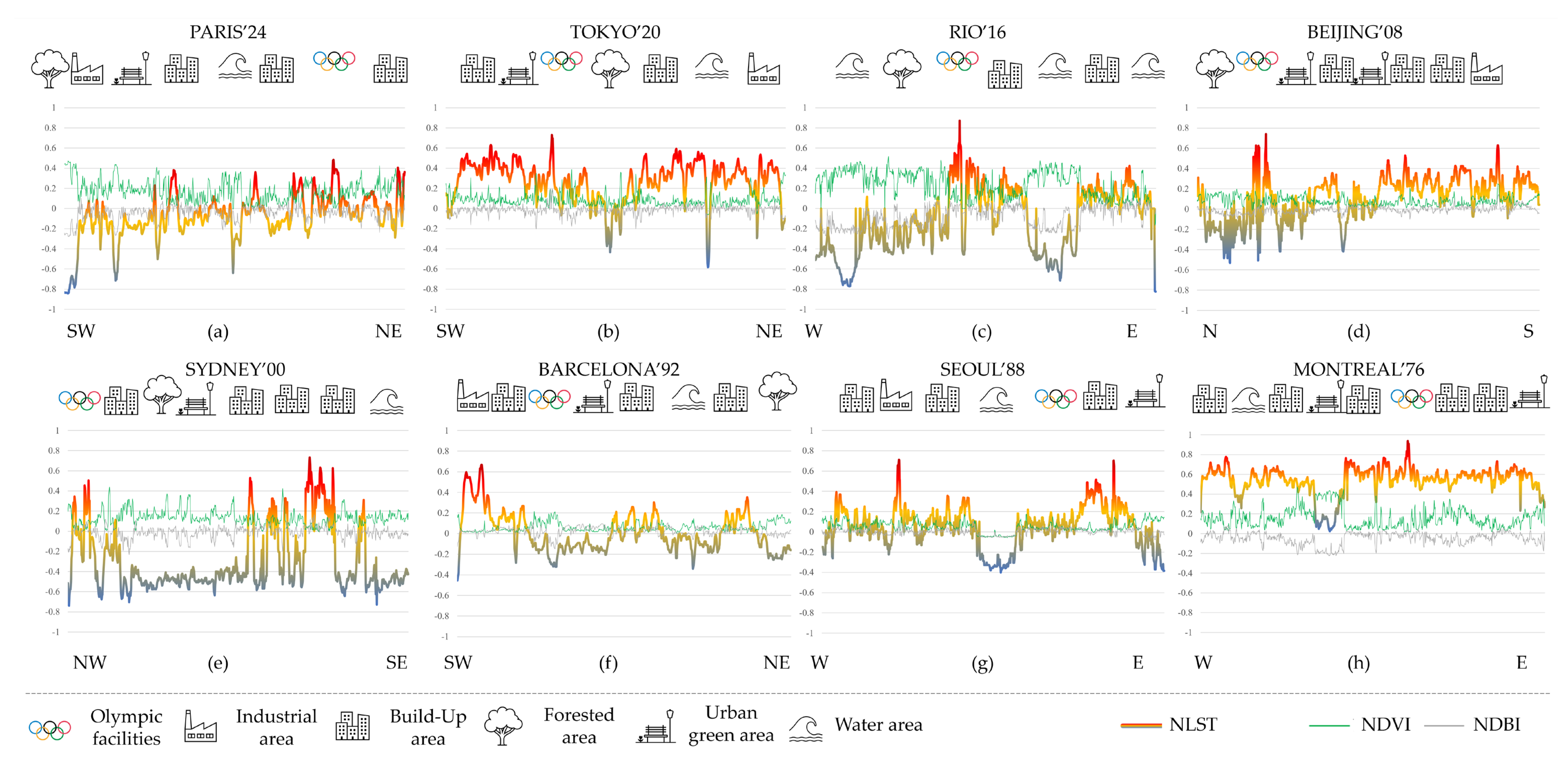
- The Paris transect has a SW to NE direction and a length of 25035 m. It was designed to sample the UHI from the point A (X: 444248, Y: 5401311) to the point B (X: 455585, Y: 5423867, EPSG: 32631) by crossing les Champs de Mars, le Montage Olympique des Invalides, the Sena River and St. Denis Stadium. In the latter, there is a peak in the NLST transect graph, indicating a hotspot in this location in relation to the Paris UHI, while in the Invalides, there is a relative green spot (Figure 8a). The clustered location of the venues, added to the combination with gardens, promotes the balancing of the heat emission of Olympic buildings.
- The Tokyo transect has a SW to NE direction with a length of 30511 m and was designed to cross the UHI from the point A (X: 375100, Y: 3941580) to the point B (X: 398083, Y: 3961660, EPSG: 32654). The sample starts at the Tama River, crosses the Yoyogi Park, the Japan National Stadium, the Tokyo Dome, the Arakawa River and finishes at the Mizumoto Park. The thermal peak is located over the Stadium and the Dome (Figure 8b). The high surface temperature reached by the Olympic building covers, added to its huge dimensions, leads to the result of an important hotspot within the city, but they are located within a green area that mitigates the heating effects.
- The Rio transect has a SW to NE direction with a length of 44230 m and it was designed to sample the UHI from the point A (X: 645756, Y:7450883) to the point B (X: 686856, Y: 7467220, EPSG: 32723). The line starts at the Portinho River estuary, crosses the Pedra Branca Park, the Olympic Village and the Barra Olimpica venue, the Tijuca National Park, and the Rio city overlapping the Maracaná Stadium. The thermal peak is located over Barra Olímpica and a secondary peak is found over Maracaná, evidencing that these kind of Olympic infrastructures are some of the higher heat emissaries in the city. The exuberant and dense vegetation of the Rio area increases the contrast between the concreted urbanized areas and its surrounding forests. This effect is still greater in the case of the Barra complex, in a peripherical location (Figure 8c).
- The Beijing transect has a S to N direction and a length of 30723 m. It was designed to cross the UHI from the point A (X: 447915, Y: 4401850) to the point B (X: 447895, Y:4432570, EPSG: 32650), starting at the Nanyuan residential district, crossing the Temple of Heaven complex, the Olympic village, the Beijing National Stadium and finishing at the Olympic Park. The coolest locations are the Olympic Park, which has a large vegetated and gardened area, and the Temple of Heaven, while the hottest is the Beijing National Stadium (Figure 8d).
- The Sydney transect has a NW to SE direction and a length of 23108 m. It was designed to cross the UHI from the point A (X: 318740, Y: 62548990) to the point B (X: 339180, Y: 6244130, EPSG: 32756). The segment starts at the Duck River, crosses the Olympic Park thorough the Accor Stadium, the residential areas of Haberfield, Macdonaldtown, Kensington and end at the sea close to South Coogee. In the case of this urban area, the extensive and low-density neighborhoods with many green spaces, contrasts with the Olympic Stadium and the central and dense downtown, where are the thermal peaks (Figure 8e). Nevertheless, the Olympic Park contains green areas and water bodies balancing the building heat.
- The Barcelona transect has a SW to NE direction and a length of 20317 m. It was designed to cross the UHI from the point A (X: 426010, Y: 4575085) to the point B (X: 438315, Y: 4591235, EPSG: 32631). The transect starts at the Llobregat River, crosses the industrial area of Mercabarna, the Olympic Ring by the Montjuïc Olympic Stadium, the densely populated old city, the Eixample, the Besós River and finishes in Badalona. The highest surface temperature is in the industrial area, and the Olympic Ring has low relative temperatures due to its vegetated park areas, such as the Botanic Garden located near to the Palau Sant Jordi and the Olympic Stadium. Similarly to the other cities, the lowest relative temperatures are over the water bodies (Figure 8f).
- The Seoul transect has a W to E direction and a length of 28530 m and it was designed to cross the UHI from the point A (X: 307545, Y: 4153195) to the point B (X: 336050, Y: 4154110, EPSG: 32652). It starts at the Bucheon Ecoaprk, crosses the densely populated areas of Dorim-Dong and Noryangjing-Dong, overlaps the Han River, enters to the Jamsil Olympic complex and the Olympic Park (where the Olympic Stadium is located), and ends at the limit with Gyeonggi-Do. As expected, the Han River presents the lowest relative surface temperatures, and the higher are located on dense urban areas and over the Olympic Stadium (Figure 8g).
- The Montreal transect has a W to E direction and a length of 28522 m. It was designed to cross the UHI from the point A (X: 605630, Y: 5030500) to the point B (X: 617910, 5056230, EPSG: 32618). Starts at the Boulevard La Salle close to the Pont Honoré-Mercier, cresses the Canal de Lachine, overlaps the residential area of Westmount, the Parc du Mont-Royal, the neighborhood of Angus, the Olympique Parc de Montral and the Stade Olympique, the low-density neighborhood of Anjou, the industrial area at East Montreal, and ends near the Île Du-Tricentenaire. The higher relative surface temperatures are found on the dense residential areas, and also it is observed a peak just over the Olympic Park; it is worth noting that the Botanic Garden, located next to the Olympic Park, and were took place the Marathon, is one of the places with lower relative surface temperature in the inner urban area. Also, the Parc du Mont-Royal and the Canal de Lachine water body are the lower thermal emissaries (Figure 8h).
Figure 8.
Transects created by using the NSLT, the NDVI and the NDBI images. It was digitized a segment crossing the city and the Olympic facilities, to obtain the thermal profile from the NLST. Also, to compare the results, it was added the NDVI and the NDBI profile. This was done with the Profile Tool QGIS plug-in, which essentially intersects the segment with the target raster, and extracts the value of the overlapped pixels. The result is a table with the values, that can be plotted in the GIS soft-ware or exported to another software (e.g. MS Excel) to edit the graph.
3.3. City Land Surface Temperatures Related to the Olympic Factilites Land Surface Temperatures.
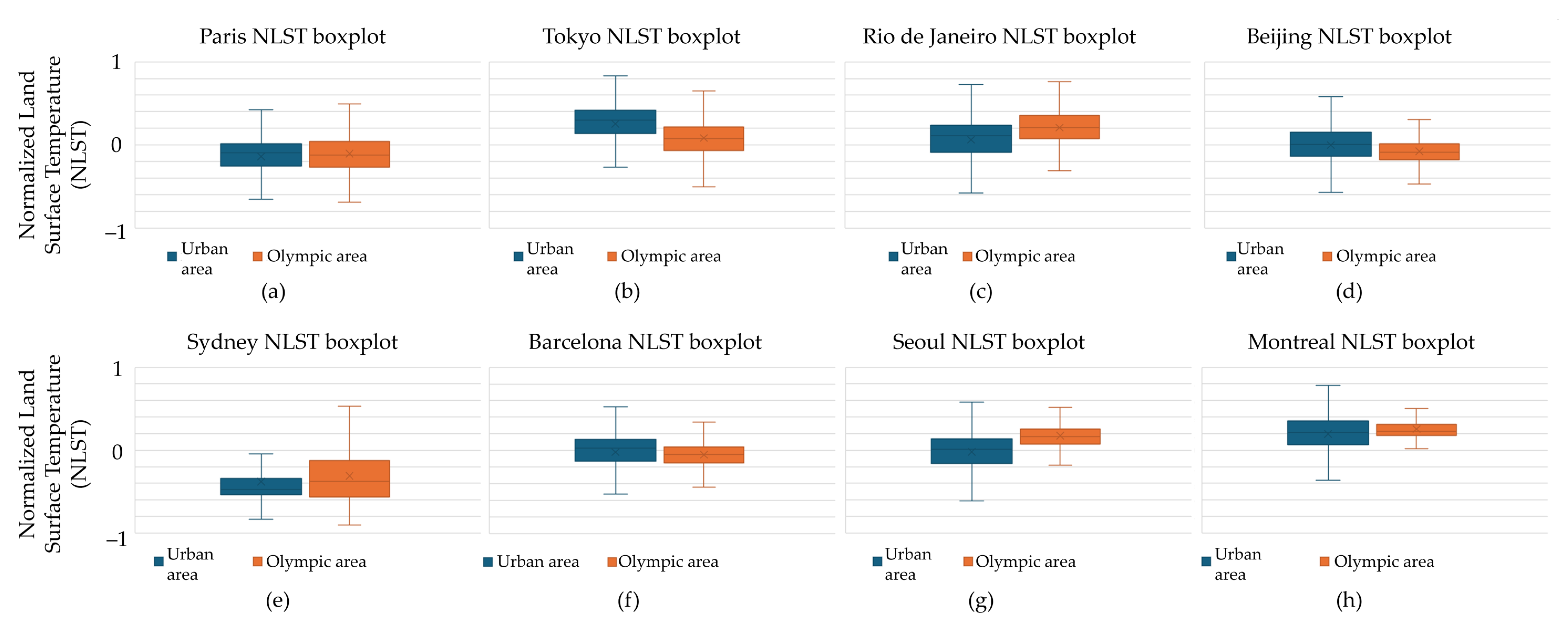
In a further explanatory analysis, and focusing on the NLST variable, we plotted the boxplot for all the pixels of each city AOI and for all the pixels within the respective Olympic facilities AOI. The boxplot excludes the outliers and values out of the range [–1 to 1]. So, the reader can summarize the data and quickly identify the distribution of LST across the areas and skewness by focusing on the quartiles and averages (Figure 9).
- Results for Paris city and its Olympic area, show a reduced interquartile range (IQR) of the NLST within the overall Paris urban in comparison to the Olympic area. This, added to a higher variability of temperatures within the Olympic area as seen in the wider distance between the minimum and the maximum, indicates that the Olympic facilities contribute to slightly increase the overall LST in the Paris urban area. The clustered location of the Olympic facilities along of the city can explain this reduced effect of hotspot in relation with its surrounded heavily urbanized area (Figure 9a).
- Findings for Tokyo city and its Olympic area, reveal a comparable IQR of the NLST within the Olympic area in comparison to the overall Tokyo urban area. The variability of temperatures within the Olympic area is also similar to the overall city, as seen in the similar distance between the minimum and the maximum. However, the median and the average LST is significantly lower in the Olympic facilities, demonstrating a strong contribution to reducing the overall LST in the Tokyo urban area. The polycentric location of the Olympic facilities along of the city can explain this effect of green spot in relation with its surrounded heavily urbanized area (Figure 9b).
- Rio city and its Olympic area, show a lower variability of the NLST in the Olympic area in relation with the overall Rio urban area as seen in the lower distance between the minimum and the maximum and between the 1st and 3rd quartile. In this case the NLST minimum, median and average values within the Olympic area are significantly higher than those in the overall Rio urban area, thus the Olympic facilities contribute to increasing the overall LST. The location of the Olympic area in the periphery of the city can explain this effect of hotspot in relation to its less heavily urbanized surrounding (Figure 9c).
- Beijing city and its Olympic area, demonstrate a shorter IQR of the NLST within the Olympic area when compared to the overall Beijing urban area. Additionally, the variability of temperatures within the Olympic area is also lower than in the overall city, as seen in the similar distance between the minimum and the maximum values. However, both the median and the average LST are lower in the Olympic facilities, showing a strong contribution to reducing the overall LST in the Beijing urban area. The fact that the Olympic facilities are located in a polycentric manner throughout the city can account for this green spot effect in relation to its surrounding heavily urbanized area (Figure 9d).
- Sydney city and its Olympic area indicate a higher variability of the NLST in the Olympic area when compared to the broader Sydney urban area. This is evident in the wider distance between the minimum and the maximum values, as well as between the 1st and 3rd quartiles. In this case the NLST median and average values within the Olympic area are much higher than in the overall urban area, thus the Olympic facilities contribute to increase the overall LST. The median and average NLST values within the Olympic area are notably higher than in the overall urban area. As a result, the Olympic facilities contribute to an increase in the overall LST. The median value is positioned closer to the bottom of the box, and the whisker on the upper end of the box is shorter, indicating a clearly negative skew in the distribution. This skew can be attributed to the mix of green spaces and hot areas within the Olympic Park. The location of the Olympic area on the periphery of the city can explain the hotspot effect, which is related to its surrounding less densely urbanized area (Figure 9e).
- The results reveals that the IQR of NLST in Barcelona’s Olympic area is shorter than in the city overall. Additionally, the variability of temperatures within the Olympic area is lower than in the rest of the city, as evidenced by the proximity of the minimum and maximum temperatures. However, the median and average LST is lower in the Olympic facilities, which significantly contributes to reducing the overall LST in the urban area of Barcelona. The fact that the Olympic facilities are clustered in a particular location within the city can explain this effect of a green spot in relation to the heavily urbanized area surrounding it (Figure 9f).
- The analysis of data for Seoul city and its Olympic area reveals a reduction in the IQR of the NLST within the Olympic area compared to the overall Seoul urban area. Additionally, there is a decrease in temperature variability within the Olympic area, as evidenced by the smaller distance between the minimum and maximum values. However, despite these findings, the average and median values, as well as the higher position of the 1st and 3rd quartiles, suggest that the Olympic facilities have led to an increase in the overall LST in the Seoul urban area. This effect can be attributed to the monocentric location of the Olympic facilities within the city and the urbanized surroundings, which creates a hot spot in relation to the overall urbanized area (Figure 9g).
- Similarly to Seoul, the data for Montreal, indicates a narrowing of the IQR of the NLST within the Olympic area as compared to the broader Montreal urban area. Additionally, the temperature variability in the Olympic Park is lower, as shown by the smaller distance between the minimum and maximum values. However, the average and median values, as well as the higher position of the 1st and 3rd quartile, suggest that the Olympic venues have contributed to an overall increase in the LST in the Montreal urban area. The central location of the Olympic facilities within the city and its urbanized surroundings can explain this effect of a hot spot in relation to the overall urbanized area (Figure 9h).
Figure 9.
Boxplots relating the Normalized Land Surface Temperature (NLST) within each urban area and within its Olympic facilities.
Figure 9.
Boxplots relating the Normalized Land Surface Temperature (NLST) within each urban area and within its Olympic facilities.
3.3. NLST Validation
The LST (K) and the NLST are expected to exhibit perfect correlation through a linear regression, as they are simply transformed using the scaling method (see 2.3.1 section). To evaluate this, we employed thermal transect pixels as samples for each city (Figure 10), achieving the expected results.
3.4. Towards a Sustainable Olympic Game Planning? Surface Thermal Mitigation Strategies
The past five decades have witnessed the development and execution of various strategies in Olympic cities. Since the Sydney 2000 Games, these strategies have aimed to achieve environmental sustainability [13]. Nevertheless, the outcomes indicate the existence of high surface temperature concentrations, necessitating the need for additional measures to supplement existing plans and attain the established objectives. Initially, the findings suggest that initiatives focused on green space management, by maintaining temperatures below average.
Emphasizing on the Olympic buildings, the urban planning has focused, especially, on proposals related to energy consumption. We believe that this propositional line is essential but can be improved, even more so when several studies indicate the direct relationship between temperatures and energy consumption in buildings [89,90]. In addition, due to low solar absorption and its impact on reducing surface temperatures [91], green roofs are also an option, even allowing to increase interior thermal comfort [92,93]. Another area of concern is the campus sports facilities, specifically in the rubber-based artificial grass fields used for sports like soccer, hockey or baseball. These materials can lead to high surface temperatures under certain meteorological conditions [94,95], even exceeding those on concrete surfaces. Substitution with natural grass is a valid option, although the current climate emergency and drought situation makes its implementation difficult (e.g. in Spain). The implementation of efficient irrigation systems would be beneficial for the establishment of urban green spaces, but if this is not feasible, temporary restrictions on the use of these facilities should be considered by the relevant authorities. A third zone of action could be established in areas with medium-high and medium temperatures, which are considered as possible transition zones. The objective of this zone would be to homogenize temperatures within ranges close to the average or even lower. The results of previous studies have shown that the coexistence of urban green spaces in are-as dominated by urbanized land uses can help to reduce temperatures. Areas of action include parking lots and particularly the surroundings of the Olympic Stadium. In terms of parking lots, most cities have implemented policies to promote sustainable mobility, reducing the use of private vehicles and public transportation. A proposal to reduce the surface area of parking spaces could be a complementary strategy, allowing for the reduction of private vehicle usage and replacing these spaces with areas of forests, gardens, or medium-height vegetation. Regarding the Olympic rings, while the passage of motorized vehicles has often been restricted during events to promote pedestrianization, we believe that it is necessary to accompany these measures with the implementation of mid-height vegetation, gardens, or awnings that can help to mitigate temperatures. Due to the influence of urban greenery, there are still opportunities to increase urban vegetation in internal and interstitial areas.
In conclusion, we recommend the implementation of vegetation in accordance with the findings of recent studies [96,97], even if it entails additional economic costs required for its correct maintenance throughout the year (irrigation, pruning, pest control, etc.). It is worth considering the idiosyncrasy of a space characterized by a significant variation in occupancy by the sports community and other massive evens, both day and night, and throughout certain seasons (holiday periods). The adaptation to climate change must prioritize the promotion of green areas rather than their reduction, especially by incorporating drought-resistant species adapted to the local habitats.
3.5 Limitations of this Study
The delimitation of urban areas can sometimes be a contentious issue, as it is influenced by disparities between the spatial boundaries of a SUHI and the administrative limits. Despite these challenges, we aimed to use the administrative limits that best suited the objectives of our study. In addition, we employed the same limits as previous studies conducted in the same city and its SUHI (e.g. Paris [98], Rio [60], Seoul [99], Montreal [100]).
Regarding the data and the cloud computing code, there is a gap affecting London’12 analysis that could be addressed with Landsat-7 data. However, due to the SLC-off failure [74] affecting this sensor and the availability of sufficient L8 data, we opted to use only the latter. Also, we used Landsat-4 and 5 for the analysis of Olympic games before 1982, instead of Lansat-1 to 3. Our criteria were guided by using the Collection 2, which is not currently available for L1 to L3. Furthermore, the spatial resolution of the thermal band on L1 to L3 was 120 meters (coarser than L4 to L9).
Finally, there are some known surface temperatures issues regarding the Collection 2, affecting the radiometric correction, the surface emissivity estimation [101], and some others related with the no data treatment or Inconsistent treatment in overlapping areas between WRS2 distribution units [102].
4. Conclusions
In this study we analysed the surface temperatures on Olympic Games facilities and the surface temperatures on its hosting city. The Olympic facilities affect to the urban climate of the hosting city, with a warming impact, but this impact has been reduced by the years thanks to new urbanistic approaches and the cohabitation with urban green spaces.
Over time, urban planners have proposed different projects that apply to the Olympic Games and its hosting cities. In the basis of five stages reflecting the history of the urban impact of the Games, we focused on the period from 1976 to 2024. The Landsat Series Collection 2 data, combined with cloud computing (e.g. Google Earth Engine) and GIS methods, allows multiple and reproducible spatiotemporal urban studies, such as the former. In this study we presented and shared a Google Earth Engine code to obtain 5-year synthetic images for eight Olympic cities (Paris’24, Tokyo’20, Rio’16, Beijing’08, Sydney’00, Barcelona’92, Seoul’88 and Montreal’76). It was analysed the contribution of the Olympic venues to the overall surface temperature of the hosting urban area. In fact, we used and validated a locally Normalized Land Surface Temperature approach to better identify the effects of the Olympic infrastructure to the Urban Heat Island, and to compare the relative surface temperature between different cities.
The results show that Olympic games urban planning affects its hosting cities, since they are centres of attraction and population concentration where land uses tend to intermingle, creating territorial complexities. These examples between Montreal’76 and Paris’24, with different urban planning patterns, evidence the role of urban greenery and how evolved its importance in the last 40 years. Our findings indicate that high surface temperatures are spatially concentrated in the concreted built-up zones around the Olympic Stadium, the Olympic village, arenas, synthetic turf courts and covered sport facilities such as domes, velodromes, or covered pools. On the other hand, open spaces with vegetation such as the equestrian parks, natural turf courts or gardens, and open aquatic waterways, are extensive areas contributing to lower temperatures. At the same time, all the cities have intrinsically urban configurations with heavily urbanized zones contributing to the urban heat, and green spaces contributing to the urban cooling. The coexistence of urban greenery like parks and gardens, with surface temperature hotspots like Olympic Stadiums and other sports complex, contributes to the mitigation urban temperatures, but also the location of the Olympic Buildings has importance. In relation to environmental policies, the Olympic urban planning has correctly evolved to more sustainable spaces, from the monocentric Olympic Parks of Montreal’76 or Seoul’88 to the polycentric distribution of Beijing’08, Tokyo’20 or Paris’24, where surface temperatures are balanced (although the Olympic Stadium is, still, the main heat contributor). Our analysis also evidence how peripheric Olympic venues such as in Sydney’00 and Rio’16 result on a relative hotspot in relation with their not urbanized areas. In general, the results confirm the need to carry out more integrative policies in spaces of transition, with the aim of improving the thermal comfort of these.
Finally, this article opens our avenues of research in relation to the behaviour of temperatures in urban and peri-urban areas. With the aim of making a greater contribution to the literature on the effect of climate change in these spaces, the GEE code tool is applicable to the coming Olympic games and to similar mega-events. Additionally, we believe that integrating Olympic infrastructures on a supra-municipal scale would help relate the temperatures that are configured within them with their peripheral spaces, thus obtaining a better understanding of the spatiality of temperatures outside dense urban areas.
Supplementary Materials
The following supporting Google Earth Engine code can be downloaded the website of this paper posted on Preprints.org: https://code.earthengine.google.com/c94283fffb394f348b37905e847fb3e5
Author Contributions
Conceptualization, J.-C.P and V.S.; methodology, J.-C.P..; software, J.-C.P.; validation, J.-C.P., R.V.-S. and M.C.-B.; formal analysis, J.-C.P and V.S.; investigation, J.-C.P and V.S.; resources, J.-C.P; data curation, J.-C.P and V.S.; writing—original draft preparation, J.-C.P.; writing—review and editing, V.S., R.V.-S. and M.C.-B.; visualization, J.-C.P.; supervision, R.V.-S.; project administration, J.-C.P; funding acquisition, J.-C.P. All authors have read and agreed to the published version of the manuscript.
Funding
This research has been funded by the Ministry of Science and Innovation in the framework of the BCN_POST_PAND project (PID2020-112734RB-C32). Secondly, this research has been funded by the Ministry of Universities and the European Union-NextGenerationEU in the framework of the Margarita Salas postdoctoral contract (Royal Decree 289/2021).
Data Availability Statement
The Google Earth Engine code can be accessed at: https://code.earthengine.google.com/45e7be760782a4177aa1abbd65c2cc22.
Acknowledgments
Landsat-4, Landsat-5, Landsat-7, Landsat-8 and Landsat-9 datasets courtesy of the U.S. Geological Survey.
Conflicts of Interest
The authors declare no conflicts of interest.
References
- Malfas, M.; Theodoraki, E.; Houlihan, B. Impacts of the Olympic Games as mega-events. Proceedings of the Institution of Civil Engineers - Municipal Engineer 2004, 157, 209–220. [CrossRef]
- della Sala, V. The Olympic Village and the Olympic Urbanism: Perception and Expectations of Olympic Specialists. Bollettino della Società Geografica Italiana 2022, 5, 51–64. [Google Scholar] [CrossRef]
- della Sala, V. The Olympic Villages and Olympic urban planning. Analysis and evaluation of the impact on territorial and urban planning (XX-XX I centuries). 2022, Doctoral thesis. UAB. POLITO. Available online: http://hdl.handle.net/10803/687631 (accessed on 14 May 2024).
- della Sala, V. Olympic Games and expectations: The factor analysis model about Olympic Urbanism and Olympic Villages. In: Sociologia e ricerca sociale, Franco Angeli: Milano, 2023, 132, 3, 127–147.
- della Sala, V. Olympic Games: Between Expectations and Fears. Factor Analysis Model Applied to Olympic Urbanism and Olympic Villages. Rivista Internazionale di Scienze Sociali 2024, 132, 55–86. [Google Scholar]
- Roche, M. Mega-Events and Micro-Modernisation: On the Sociology of the New Urban Tourism. British Journal of Sociology 1992, 43, 563–600. [Google Scholar] [CrossRef]
- Roche, M. Mega-events and Modernity: Olympics and Expos in the Growth of Global C. Routledge: London. 2000.
- Roche, M. Olympic and Sport Mega-Events as Media-Events: Reflections on the Globalisation paradigm. Symposium A Quarterly Journal in Modern Foreign Literatures 2002, 1–12. Available online: https://citeseerx.ist.psu.edu/document?repid=rep1&type=pdf&doi=1bbe07c9a1b53747a55c8db4d220a4072428faf8 (accessed on 14 May 2024).
- Roche, M. The Olympics and the Development of "Global Society". In: M. De Moragas, C. Kennett, N. Puig, The Legacy of the Olympic Games, Document of the Olympic Museum, International Olympic Committee, Lausanne, 2003.
- Roche, M. Mega-Events and Modernity Revisited: Globalization and the Case of the Olympics. The Sociological Review 2006, 54, 27–40. [Google Scholar] [CrossRef]
- Rose, A.K.; M. Spiegel. The Olympic Effect. National Bureau of Economic Research, 2009. Available online: https://www.nber.org/system/files/working_papers/w14854/w14854.pdf (accessed on 14 May 2024).
- Essex, S.; Chalkley, B. Olympic games: Catalyst of urban change. Leisure Studies 1998, 17, 187–206. [Google Scholar] [CrossRef]
- Dunn, M.K.; McGuirk, M.P. Hallmark events. In: Staging the Olympics: The Event and its Impacts, Cashman, R. and Hughes, A. Eds. Centre for Olympic Studies, UNSW, Sydney, 1999.
- Moragas, M. Olympic villages: a hundred years of urban planning and shared experiences: International Symposium on Olympic Villages. In: Centre d’Estudis Olímpics i de l’Esport Universitat Autònoma de Barcelona; Olympic Museum (Ed.), Olympic Villages Hundred Years of Urban Planning and Shared Experiences. Lausanne, 1996.
- Georgiadis, K.; Theodorikakos, P. The Olympic Games of Athens: 10 years later. Sport in Society 2015, 19, 817–827. [Google Scholar] [CrossRef]
- Jia, H.; Lu, Y.; Yu, S. L.; Chen, Y. Planning of LID-BMPs for urban runoff control: The case of Beijing Olympic Village. Separation and Purification Technology 2012, 84, 112–119. [Google Scholar] [CrossRef]
- Imrie, R.; Lees, L.; Raco, M. Regenerating London: Governance, Sustainability and Community in a Global City. Routledge: London. 2008.
- Cook, I. G.; Miles, S. Beijing 2008: Chapter taken from Olympic Cities. Routledge Online Studies on the Olympic and Paralympic Games, 1(36), 340–358. 2012.
- Bokaie, M.; Zarkesh, M.K.; Arasteh, P.D.; Hosseini, A. Assessment of Urban Heat Island based on the relationship between land surface temperature and Land Use/ Land Cover in Tehran. Sustainable Cities and Society 2016, 23, 94–104. [Google Scholar] [CrossRef]
- Fashae, O.A.; Adagbasa, E.G.; Olusola, A.O.; Obateru, R.O. Land use/land cover change and land surface temperature of Ibadan and environs, Nigeria. Environ. Monit. Assess. 2020, 192, 109. [Google Scholar] [CrossRef] [PubMed]
- IPCC [Intergovernmental Panel on Climate Change]. Glossary. In: Climate Change 2022 – Impacts, Adaptation and Vulnerability: Working Group II Contribution to the Sixth Assessment Report of the Intergovernmental Panel on Climate Change. Cambridge University Press; 2023:2897-2930. [CrossRef]
- European Environment Agency. Urban adaptation in Europe: How cities and towns respond to climate change. Publications Office of the European Union 2020. Available online: https://data.europa.eu/doi/10.2800/324620 (accessed on 14 May 2024).
- Santamouris, M. Urban climate change: Reasons, magnitude, impact, and mitigation. In: Urban Climate Change and Heat Islands. Riccardo Paolini, Matthaios Santamouris, Eds.; Elsevier: Amsterdam, Netherlands 2023; pp. 1–27. [CrossRef]
- Chun, B.; Guldmann, J.-M. Impact of greening on the urban heat island: Seasonal variations and mitigation strategies. Computers, Environment and Urban Systems 2018, 71, 165–176. [Google Scholar] [CrossRef]
- Dwivedi, A.; Mohan, B.K. Impact of green roof on micro climate to reduce Urban Heat Island. Remote Sensing Applications: Society and Environment 2018, 10, 56–69. [Google Scholar] [CrossRef]
- Leal Filho, W.; Wolf, F.; Castro-Díaz, R.; Li, C.; Ojeh, V.N.; Gutiérrez, N.; Nagy, G.J.; Savić, S.; Natenzon, C.E.; Quasem Al-Amin, A.; et al. Addressing the Urban Heat Islands Effect: A Cross-Country Assessment of the Role of Green Infrastructure. Sustainability 2021, 13, 753. [Google Scholar] [CrossRef]
- Herath, H.M.P.I.K.; Halwatura, R.U.; Jayasinghe, G.Y. Evaluation of green infrastructure effects on tropical Sri Lankan urban context as an urban heat island adaptation strategy. Urban Forestry & Urban Greening 2018, 29, 212–222. [Google Scholar] [CrossRef]
- Herrera-Gómez, S.S.; Quevedo-Nolasco, A.; Pérez-Urrestarazu, L. The role of green roofs in climate change mitigation: A case study in Seville (Spain). Building and Environment 2017, 123, 575–584. [Google Scholar] [CrossRef]
- Abdulateef, M.F.; Al-Alwan, H.A.S. The effectiveness of urban green infrastructure in reducing surface urban heat island: Baghdad city as a case study. Ain Shams Engineering Journal 2022, 13, 101526. [Google Scholar] [CrossRef]
- Maimaitiyiming, M.; Ghulam, A.; Tiyip, T.; Pla, F.; Latorre-Carmona, P.; Halik, Ü.; Sawut, M.; Caetano, M. Effects of green space spatial pattern on land surface temperature: Implications for sustainable urban planning and climate change adaptation. ISPRS J. Photogramm. Remote Sens. 2014, 89, 59–66. [Google Scholar] [CrossRef]
- Andrade, H.; Vieira, R. A climatic study of an urban green space: The Gulbenkian Park in Lisbon (Portugal). Finisterra: Revista Portuguesa de Geografia 2007, 42, 27–46. [Google Scholar] [CrossRef]
- Jiang, J.; Tian, G. Analysis of the impact of Land use/Land cover change on Land Surface Temperature with Remote Sensing. Procedia Environmental Sciences 2010, 2, 571–575. [Google Scholar] [CrossRef]
- Tran, H.; Uchihama, D.; Ochi, S.; Yasuoka, Y. Assessment with satellite data of the urban heat island effects in Asian mega cities. International Journal of Applied Earth Observation and Geoinformation 2006, 8, 34–48. [Google Scholar] [CrossRef]
- Yang, J.; Yu, Q.; Gong, P. Quantifying air pollution removal by green roofs in Chicago. Atmospheric Environment 2008, 42, 7266–7273. [Google Scholar] [CrossRef]
- Battista, G.; Evangelisti, L.; Guattari, C.; De Lieto Vollaro, E.; De Lieto Vollaro, R.; Asdrubali, F. Urban Heat Island Mitigation Strategies: Experimental and Numerical Analysis of a University Campus in Rome (Italy). Sustainability 2020, 12, 7971. [Google Scholar] [CrossRef]
- Shashua-Bar, L.; Hoffman, M.E.; Tzamir, Y. Integrated thermal effects of generic built forms and vegetation on the UCL microclimate. Building and Environment 2006, 41, 343–354. [Google Scholar] [CrossRef]
- Wong, N.H.; Cheong, D.K. W.; Yan, H.; Soh, J.; Ong, C.L.; Sia, A. The effects of rooftop garden on energy consumption of a commercial building in Singapore. Energy and Buildings 2003, 35, 353–364. [Google Scholar] [CrossRef]
- Yang, B.; Liu, H.; Kang, E.L. Traffic restrictions during the 2008 Olympic Games reduced urban heat intensity and extent in Beijing. Commun Earth Environ 2022, 105–115. [Google Scholar] [CrossRef]
- Vicente-Salar, R.; Castelló-Bueno, M.; Logan, S.; Padró, J.-C. Efecto de los usos y las cubiertas del suelo y las políticas ambientales en el comportamiento de las temperaturas superficiales en campus universitarios. El caso de la Universitat Autònoma de Barcelona. Documents d’Anàlisi Geogràfica 2024, 70, 261–289. [Google Scholar] [CrossRef]
- Cai, G.; Liu, Y.; Du, M. Impact of the 2008 Olympic Games on urban thermal environment in Beijing, China from satellite images.
- Sustainable Cities and Society 2017, 32, 212–225. [CrossRef]
- Do, J.; Ahn, S.; Kang, J. Urbanization effect of mega sporting events using sentinel-2 satellite images: The case of the pyeongchang olympics. Sustainable Cities and Society 2021, 74, 103158. [Google Scholar] [CrossRef]
- Tu, Y.; Chen, B.; Yang, J.; Xu, B. Olympic effects on reshaping urban greenspace of host cities. Landscape and Urban Planning 2023, 230, 104615. [Google Scholar] [CrossRef]
- AEMET [Agencia Estatal de Meteorología]. Redes de observación de superficie y en altura. Redes de observación de superficie y en altura. Available online: www.aemet.es/ca/idi/observacion/observacion_convencional (accessed on 14 May 2024).
- METEOCAT [Servei Meteorològic de Catalunya]. Dades d’estacions meteorològiques automàtiques de Catalunya: Mapa d’estacions automàtiques. Available online: https://www.meteo.cat/observacions/xema (accessed on 14 May 2024).
- EUMETSAT [European Organization for the Exploitation of Meteorological Satellites]. Meteosat series. Available online: https://www.eumetsat.int/our-satellites/meteosat-series (accessed on 14 May 2024).
- NASA [National Aeronautics and Space Administration]. ARSET - Satellite Remote Sensing for Urban Heat Islands. Available online: https://appliedsciences.nasa.gov/get-involved/training/english/arset-satellite-remote-sensing-measuring-urban-heat-islands-and (accessed on 14 May 2024).
- Maharjan, M.; Aryal, A.; Man Shakya, B.; Talchabhadel, R.; Thapa, B.R.; Kumar, S. Evaluation of Urban Heat Island (UHI) Using Satellite Images in Densely Populated Cities of South Asia. Earth 2021, 2, 86–110. [Google Scholar] [CrossRef]
- Xian, G.; Gallo, K. Islas de Calor Urbano Observadas a partir de una Serie Temporal de Datos de Teledetección. Applied Remote Sensing Training Program National Aeronautics and Space Administration 2020. Available online: https://appliedsciences.nasa.gov/sites/default/files/2020-11/UHI_Part3_Xian_Span.pdf (accessed on 14 May 2024).
- Del Pozo, S.; Landes, T.; Nerry, F.; Kastendeuch, P.; Najjar, G.; Philipps, N.; Lagüela, S. UHI estimation based on aster and MODIS satellite imagery: first results on Strasbourg city, France. The International Archives of the Photogrammetry, Remote Sensing and Spatial Information Sciences 2020, XLIII-B3-2020, 799–805. [Google Scholar] [CrossRef]
- Soto-Soto, J.E.; Garzon-Barrero, J.; Jimenez-Cleves, G. Análisis de islas de calor urbano usando imágenes Landsat caso de estudio Armenia-Colombia 1996-2018. Revista Espacios 2020, 41, 9. Available online: https://www.revistaespacios.com/a20v41n08/a20v41n08p09.pdf (accessed on 14 May 2024).
- Aragón, J.A.; Rodríguez, E.D.; Varon, G.A.; Sánchez, G.A. Análisis de islas de calor por medio de imágenes satelitales y sistemas de información geográficos en el área urbana de la Sabana de Bogotá. Geographicalia 2020, 72, 39–64. [Google Scholar] [CrossRef]
- Sucapuca Mamani, R.O.; Choquehuanca Soto, J.D.; Pelinco Ruedas, E. Islas de calor urbano mediante imágenes satelitales en la ciudad de Juliaca durante el año 2019. Ciencia & Desarrollo 2022, 21, 10–28. [Google Scholar] [CrossRef]
- USGS [United States Geological Survey] (2022). Landsat Series. Available online: https://www.usgs.gov/landsat-missions (accessed on 14 May 2024).
- Sobrino, J.A.; Jiménez-Muñoz, J. Land surface temperature retrieval from thermal infrared data: An assessment in the context of the Surface Processes and Ecosystem Changes Through Response Analysis (SPECTRA) mission. Journal of Geophysical Research 2005, 110, D16103. [Google Scholar] [CrossRef]
- Ermida, S.L.; Soares, P.; Mantas, V.; Göttsche, F.-M.; Trigo, I.F. Google Earth Engine Open-Source Code for Land Surface Temperature Estimation from the Landsat Series. Remote Sens. 2020, 12, 1471. [Google Scholar] [CrossRef]
- Hidalgo-García, D.; Arco-Díaz, J. Spatial and Multi-Temporal Analysis of Land Surface Temperature through Landsat 8 Images: Comparison of Algorithms in a Highly Polluted City (Granada). Remote Sens. 2021, 13, 1012. [Google Scholar] [CrossRef]
- Sheng, L.; Tang, X.; You, H.; Gu, Q.; Hu, H. Comparison of the urban heat island intensity quantified by using air temperature and Landsat land surface temperature in Hangzhou, China. Ecological Indicators 2017, 72, 738–746. [Google Scholar] [CrossRef]
- Yi, T.; Wang, H.; Liu, C.; Li, X.; Wu, J. Thermal comfort differences between urban villages and formal settlements in Chinese developing cities: A case study in Shenzhen. Science of The Total Environment 2022, 853, 158283. [Google Scholar] [CrossRef] [PubMed]
- Mohamadi, B.; Chen, S.; Balz, T.; Gulshad, K.; McClure, S.C. Normalized Method for Land Surface Temperature Monitoring on Coastal Reclaimed Areas. Sensors 2019, 19, 4836. [Google Scholar] [CrossRef] [PubMed]
- Peres, L.; de Lucena, A.J.; Rotunno, O.; de Almeida, J.R. The urban heat island in Rio de Janeiro, Brazil, in the last 30 years using remote sensing data. IJAEO 2018, 64, 104–116. [Google Scholar] [CrossRef]
- Amiri, R.; Weng, Q.; Alimohammadi, a.; Alavipanah, S.K. Spatial–temporal dynamics of land surface temperature in relation to fractional vegetation cover and land use/cover in the Tabriz urban area, Iran. Remote Sensing of Environment 2009, 113, 2606–2617. [Google Scholar] [CrossRef]
- Haashemi, S.; Weng, Q.; Darvishi, A.; Alavipanah, S.K. Seasonal Variations of the Surface Urban Heat Island in a Semi-Arid City. Remote Sens. 2016, 8, 352. [Google Scholar] [CrossRef]
- International Olympic Committee (IOC). Olympic Games. Available online: https://olympics.com/en/olympic-games (accessed on 14 May 2024).
- Global Administrative Boundaries (GADM). GADM maps and data. Available online: https://gadm.org/ (accessed on 14 May 2024).
- QGIS plugins. HCMGIS. Available online: https://plugins.qgis.org/plugins/HCMGIS/ (accessed on 14 May 2024).
- Institut National de la statistique et des Études Économiques (INSEE). Estimation de la population au 1ᵉʳ janvier 2023 Séries par région, département, sexe et âge. Available online: https://www.insee.fr/fr/statistiques/1893198 (accessed on 14 May 2024).
- City Population. Major agglomerations of the world. Available online: https://www.citypopulation.de/en/world/agglomerations/ (accessed on 14 May 2024).
- Instituto Brasileiro de Geografia e Estatística (IBGE). Cidades e Estados: Rio de Janeiro. Available online: https://www.ibge.gov.br/cidades-e-estados/rj/rio-de-janeiro.html (accessed on 14 May 2024).
- The People’s Government of Beijing Municipality. Beijing Population. Available online: https://english.beijing.gov.cn/beijinginfo/facts/202006/t20200601_1912283.html (accessed on 14 May 2024).
- Australian Bureau of Statistics (ABS). Population Projections, Australia. Available online: https://www.abs.gov.au/statistics/people/population/regional-population/2022-23 (accessed on 14 May 2024).
- Statistical Institute of Catalonia (IDESCAT). Barcelona (Barcelonès). Available online: https://www.idescat.cat/emex/?lang=en&id=080193 (accessed on 14 May 2024).
- Seoul Metropolitan Government. City Overview. Available online: https://english.seoul.go.kr/seoul-views/meaning-of-seoul/4-population/ (accessed on 14 May 2024).
- Statistics Canada. Census Profile, 2021 Census of Population. Available online: https://www12.statcan.gc.ca/census-recensement/2021/dp-pd/prof/index.cfm?Lang=E (accessed on 14 May 2024).
- USGS [United States Geological Survey] (2023a). What are the band designations for the Landsat satellites? Available online: https://www.usgs.gov/faqs/what-are-band-designations-landsat-satellites (accessed on 14 May 2024).
- USGS [United States Geological Survey] (2023b). Landsat 7. Available online: https://www.usgs.gov/landsat-missions/landsat 7 (accessed on 14 May 2024).
- Earth Engine Data Catalog (2024a). USGS Landsat 4 Level 2, Collection 2, Tier 1. Available online: https://developers.google.com/earth-engine/datasets/catalog/LANDSAT_LT04_C02_T1_L2 (accessed on 14 May 2024).
- Earth Engine Data Catalog (2024b). USGS Landsat 5 Level 2, Collection 2, Tier 1. Available online: https://developers.google.com/earth-engine/datasets/catalog/LANDSAT_LT05_C02_T1_L2 (accessed on 14 May 2024).
- Earth Engine Data Catalog (2024c). USGS Landsat 7 Level 2, Collection 2, Tier 1. Available online: https://developers.google.com/earth-engine/datasets/catalog/LANDSAT_LE07_C02_T1_L2 (accessed on 14 May 2024).
- Earth Engine Data Catalog (2024d). USGS Landsat 8 Level 2, Collection 2, Tier 1. Available online: https://developers.google.com/earth-engine/datasets/catalog/LANDSAT_LC08_C02_T1_L2 (accessed on 14 May 2024).
- Earth Engine Data Catalog (2024e). USGS Landsat 9 Level 2, Collection 2, Tier 1. Available online: https://developers.google.com/earth-engine/datasets/catalog/LANDSAT_LC09_C02_T1_L2 (accessed on 14 May 2024).
- NASA [National Aeronautics and Space Administration]. Landsat Science: The Worldwide Reference System. Available online: https://landsat.gsfc.nasa.gov/about/the-worldwide-reference-system/ (accessed on 14 May 2024).
- USGS [United States Geological Survey] (2023a). Landsat Collection 2 Surface Temperature. Available online: www.usgs.gov/landsat-missions/landsat-collection-2-surface-temperature (accessed on 14 May 2024).
- Díaz-Delgado, R.; Pons, X. Spatial patterns of forest fires in Catalonia (NE of Spain) along the period 1975–1995: analysis of vegetation recovery after fire. Forest Ecology and Manag. 2001, 147, 67–74. [Google Scholar] [CrossRef]
- Google Developers. Machine Learning Foundational Courses: Normalization. Available online: https://developers.google.com/machine-learning/data-prep/transform/normalization (accessed on 14 May 2024).
- Skelhorn, C.; Lindley, S.; Levermore, G. The impact of vegetation types on air and surface temperatures in a temperate city: A fine scale assessment in Manchester, UK. Landscape and Urban Planning 2014, 121, 129–140. [Google Scholar] [CrossRef]
- QGIS Development Team. QGIS Geographic Information System 3.32. Open-Source Geospatial Foundation Project. Available online: http://qgis.osgeo.org (accessed on 14 May 2024).
- Sfakianaki, A.; Pagalou, E.; Pavlou, K.; Santamouris, M.; Assimakopoulos, M.N. Theoretical and experimental analysis of the thermal behaviour of a green roof system installed in two residential buildings in Athens, Greece. International Journal of Energy Research 2009, 33, 1059–1069. [Google Scholar] [CrossRef]
- QGIS plugins. Profile Tool. Available online: https://plugins.qgis.org/plugins/profiletool/ (accessed on 14 May 2024).
- Kumari, P.; Kapur, S.; Garg, V.; Kumar, K. Effect of Surface Temperature on Energy Consumption in a Calibrated Building: A Case Study of Delhi. Climate 2020, 8, 71. [Google Scholar] [CrossRef]
- Fung, W.; Lam, K.; Hung, W.; Pang, S.; Lee, Y. Impact of urban temperature on energy consumption of Hong Kong. Energy 2006, 31, 2623–2637. [Google Scholar] [CrossRef]
- Susca, T.; Gaffin, S.R.; Dell’Osso, G.R. Positive effects of vegetation: Urban heat island and green roofs. Environmental Pollution 2011, 159, 2119–2126. [Google Scholar] [CrossRef] [PubMed]
- Kim, J.; Lee, S. Y.; Kang, J. Temperature Reduction Effects of Rooftop Garden Arrangements: A Case Study of Seoul National University. Sustainability 2020, 12, 6032. [Google Scholar] [CrossRef]
- Razzaghmanesh, M.; Beecham, S.; Salemi, T. The role of green roofs in mitigating Urban Heat Island effects in the metropolitan area of Adelaide, South Australia. Urban Forestry & Urban Greening 2016, 15, 89–102. [Google Scholar] [CrossRef]
- Jia, X.; Dukes, M.D.; Miller, G.L. Temperature Increase on Synthetic Turf Grass. World Environmental and Water Resources Congress 2007, 1–20. [Google Scholar] [CrossRef]
- Thoms, A. W.; Brosnan, J. T.; Zidek, J. M.; Sorochan, J. C. Models for Predicting Surface Temperatures on Synthetic Turf Playing Surfaces. Procedia Engineering 2014, 72, 895–900. [Google Scholar] [CrossRef]
- Guo, A.; He, T.; Yue, W.; Xiao, W.; Yang, J.; Zhang, M.; Li, M. Contribution of urban trees in reducing land surface temperature: Evidence from China’s major cities. International Journal of Applied Earth Observation and Geoinformation 2023, 125, 103570. [Google Scholar] [CrossRef]
- Balany, F.; Ng, A.W.; Muttil, N.; Muthukumaran, S.; Wong, M.S. Green infrastructure as an urban heat island mitigation strategy—A review. Water 2020, 12, 3577. [Google Scholar] [CrossRef]
- De Ridder, K.; Maiheu, B.; Lauwaet, D.; Daglis, I.A.; Keramitsoglou, I.; Kourtidis, K.; Manunta, P.; Paganini, M. Urban Heat Island Intensification during Hot Spells—The Case of Paris during the Summer of 2003. Urban Sci. 2017, 1, 3. [Google Scholar] [CrossRef]
- Ngarambe, J.; Santamouris, M.; Yun, G.Y. The Impact of Urban Warming on the Mortality of Vulnerable Populations in Seoul. Sustainability 2022, 14, 13452. [Google Scholar] [CrossRef]
- Mirzaei, P.; Olsthoorn, D.; Torjan, M.; Haghighat, F. Urban neighborhood characteristics influence on a building indoor environment. Sustainable Cities and Society 2015, 19, 403–417. [Google Scholar] [CrossRef]
- USGS [United States Geological Survey]. Landsat Collection 2 known issues. Available online: https://www.usgs.gov/landsat-missions/landsat-collection-2-known-issues#ST (accessed on 14 May 2024).
- Pons, X.; Cea, C.; González-Guerrero, O.; Cristóbal, J. Consideraciones sobre la colección 2 de Landsat. In: XX Congreso de la Asociación Española de Teledetección. Eds. Caballero, I.; Navarro, G.; Barbero, L; Gómez-Enri, J. 2024, Cádiz, Spain.
Figure 1.
Location of the Olympic Game cities from 1972 to 2024, which are included in the Google Earth Engine code. Highlighted (yellow) the cities used as examples in this paper, representing four Olympic urban planning patterns. Source: Own elaboration based on data from the Open Street Maps and the International Olympic Committee (IOC) information [63].
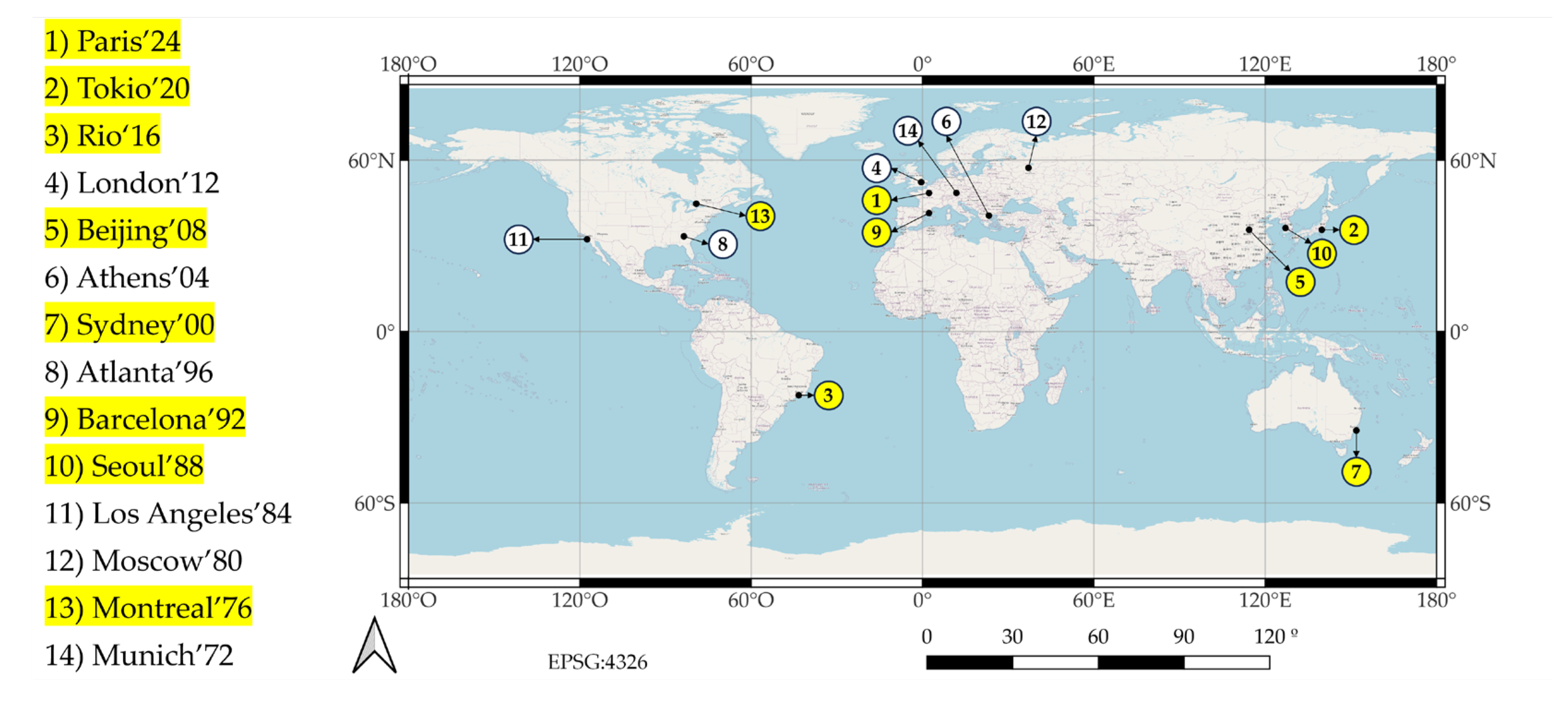
Figure 2.
Area Of Interest (City AOI) of the eight cities analysed (red outline), and its corresponding Area Of Interest (Olympic AOI) of the Olympic facilities (yellow outline). (a) In the Paris case, the City AOI is defined by the Ille de France administrative boundaries. (b) In the Tokyo case, the City AOI is defined by some municipalities of the Tokyo Metropolitan Area administrative boundaries. (c) In the Rio case, the City AOI is defined by the Rio de Janeiro Municipality administrative boundaries. (d) In the Beijing case, the City AOI is defined Beijing Municipality administrative boundaries. (e) In the Sydney case, the City AOI is defined by some municipalities of North South Wales administrative boundaries. (f) In the Barcelona case, the City AOI is defined by Barcelonès administrative boundaries. (g) In the Seoul case, the City AOI is defined by Keijo Teukbyeolsi administrative boundaries. (h) In the Montreal case, the City AOI is defined by the Champlain, Communauté-Urbaine-de-Montréal and Laval administrative boundaries.
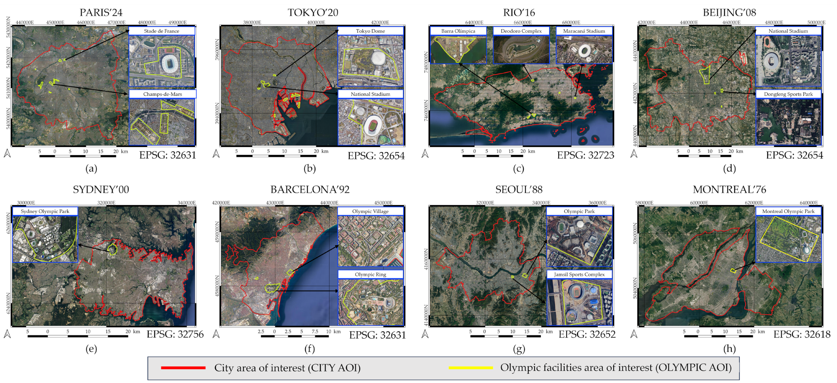
Figure 3.
Overall methodology and processing chain.
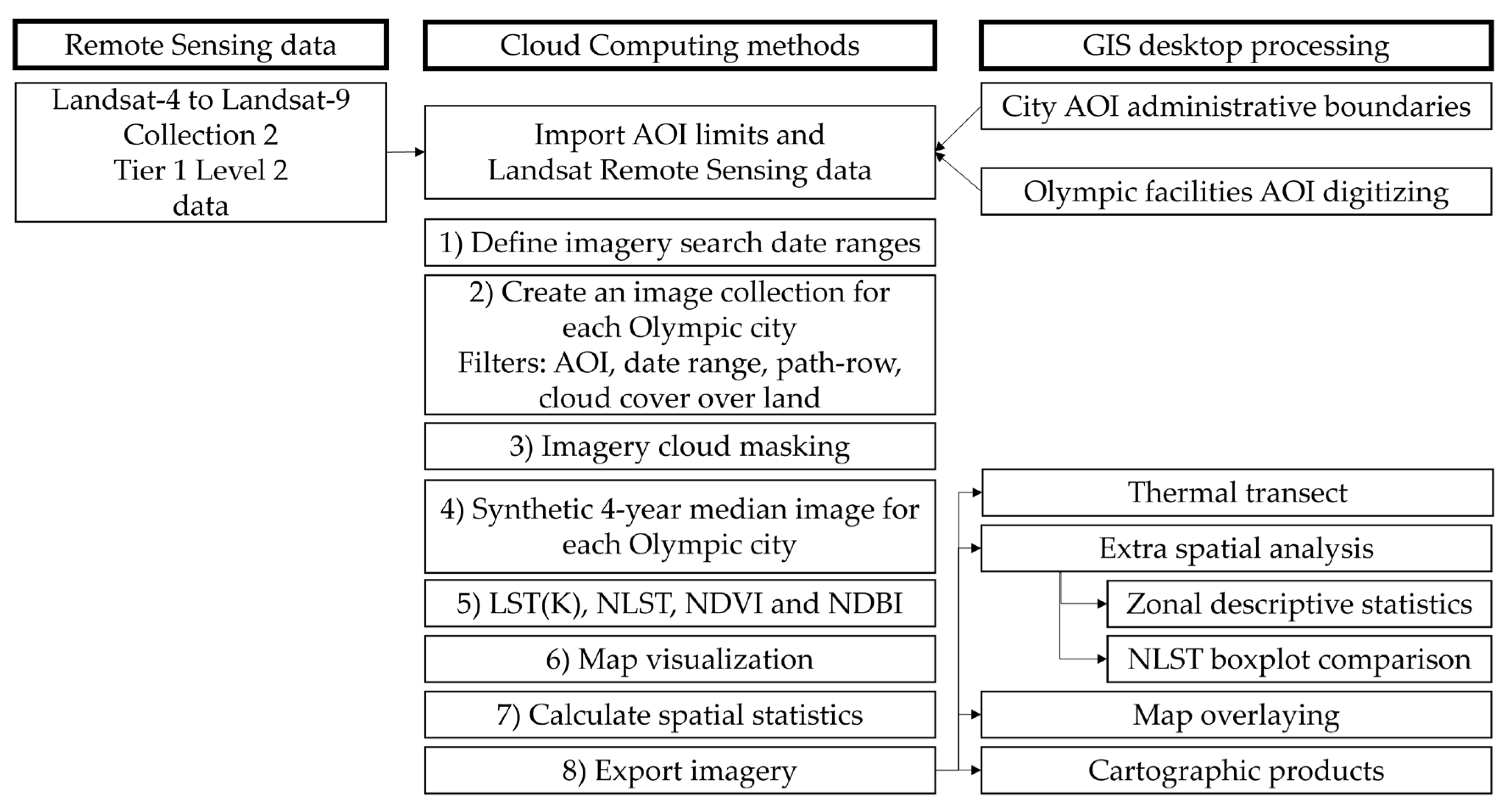
Figure 4.
Area Of Interest (City AOI) of the eight cities analysed (red outline), and its corresponding Area Of Interest (Olympic AOI) of the Olympic facilities (yellow outline). (a) In the Paris case, the City AOI is defined by the Ille de France administrative boundaries. (b) In the Tokyo case, the City AOI is defined by some municipalities of the Tokyo Metropolitan Area administrative boundaries. (c) In the Rio case, the City AOI is defined by the Rio de Janeiro Municipality administrative boundaries. (d) In the Beijing case, the City AOI is defined Beijing Municipality administrative boundaries. (e) In the Sydney case, the City AOI is defined by some municipalities of North South Wales administrative boundaries. (f) In the Barcelona case, the City AOI is defined by Barcelonès administrative boundaries. (g) In the Seoul case, the City AOI is defined by Keijo Teukbyeolsi administrative boundaries. (h) In the Montreal case, the City AOI is defined by the Champlain, Communauté-Urbaine-de-Montréal and Laval administrative boundaries.
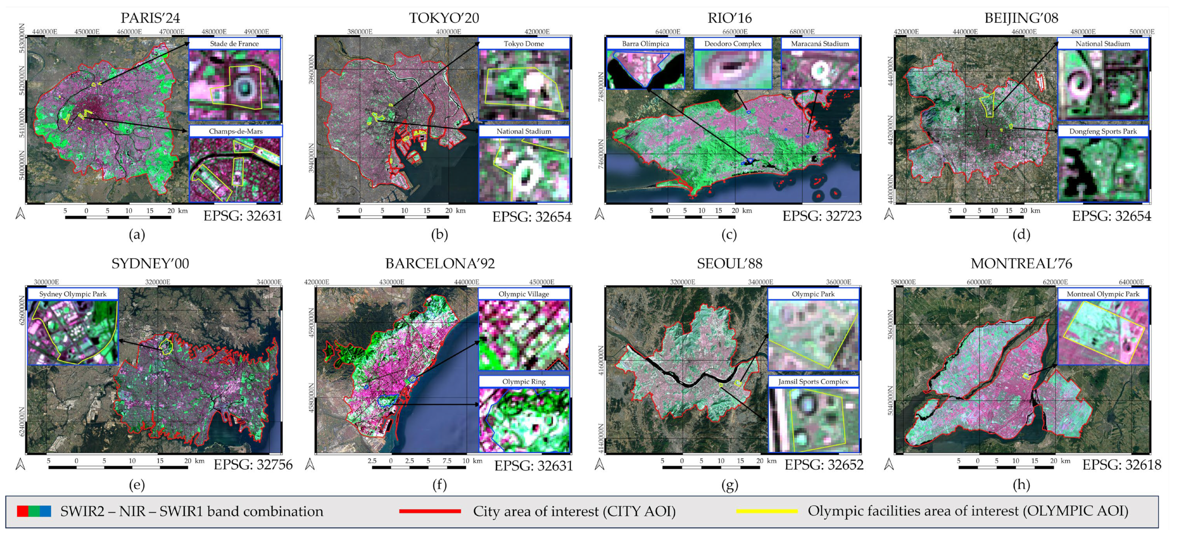
Figure 5.
Normalized Difference Vegetation Index (NDVI) maps created by using the median synthetic image of 5-year period, for each of the 8 cities analysed in this study. NDVI was calculated using NIR and RED bands of the synthetic image (see eq. 3). Also, focus on the main Olympic facilities. The real data range is [-1 to 1], but for a better understanding and visualization it was stretched to [-0.25 to 0.25] in all the maps.
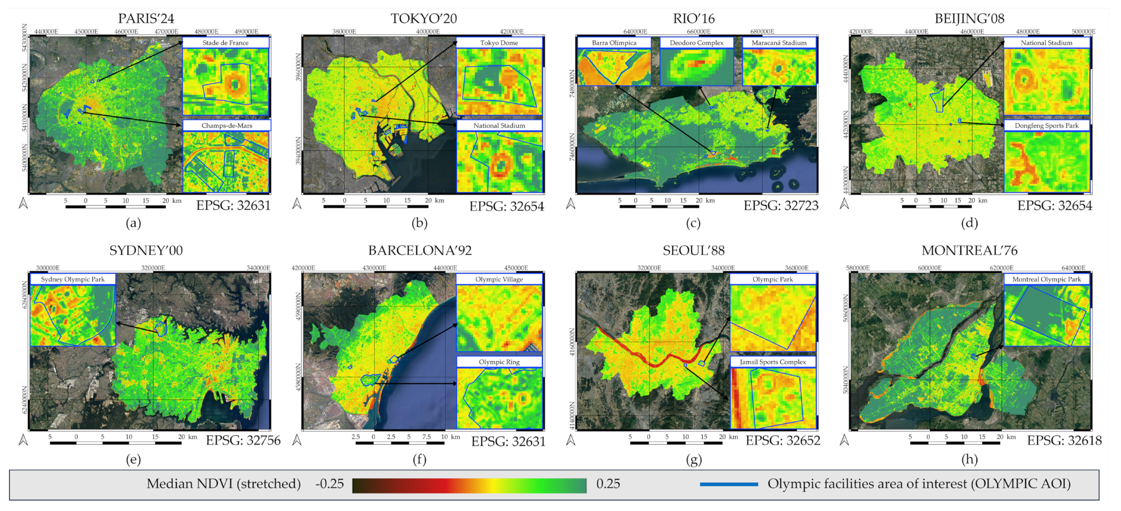
Figure 6.
Normalized Difference Built-Up Index (NDBI) maps created by using the median synthetic image of 5-year period, for each of the 8 cities analysed in this study. NDBI was calculated using NIR and SWIR1 bands of the synthetic image (see eq. 4). Also, focus on the main Olympic facilities. The real data range is [–1 to 1], but for a better understanding and visualization it was stretched to [–0.25 to 0.25] in all the maps.
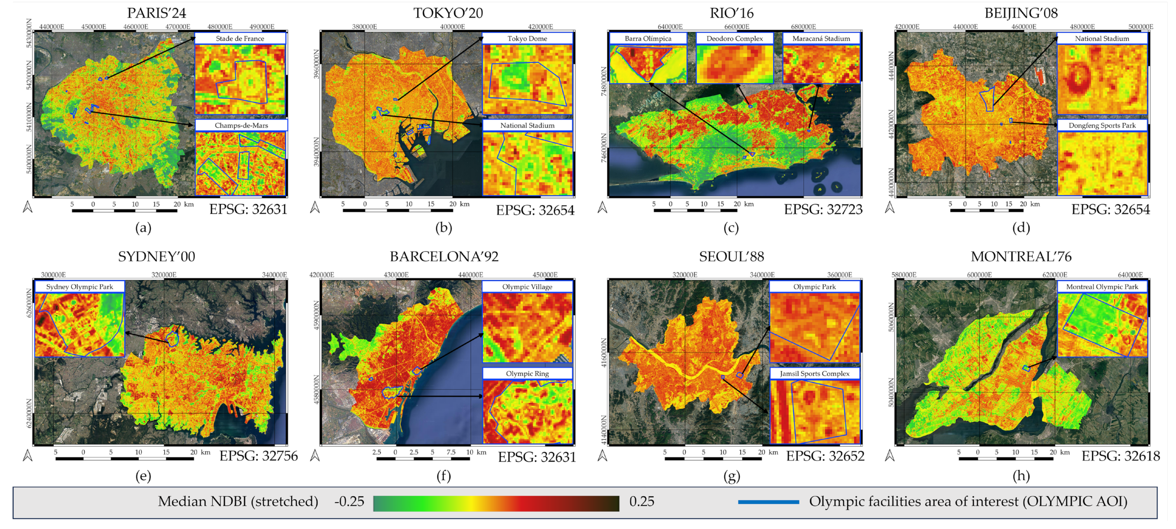
Figure 7.
Normalized Land Surface Temperature (NLST) maps created by using the median synthetic image of 5-year period, for each of the 8 cities analysed in this study. NLST was calculated using the Thermal band of the synthetic image, and the minimum and maximum LST values in each city (see eq. 4). Also, focus on the main Olympic facilities, and it is added the transect used to calculate the thermal profile of the NLST in each city.
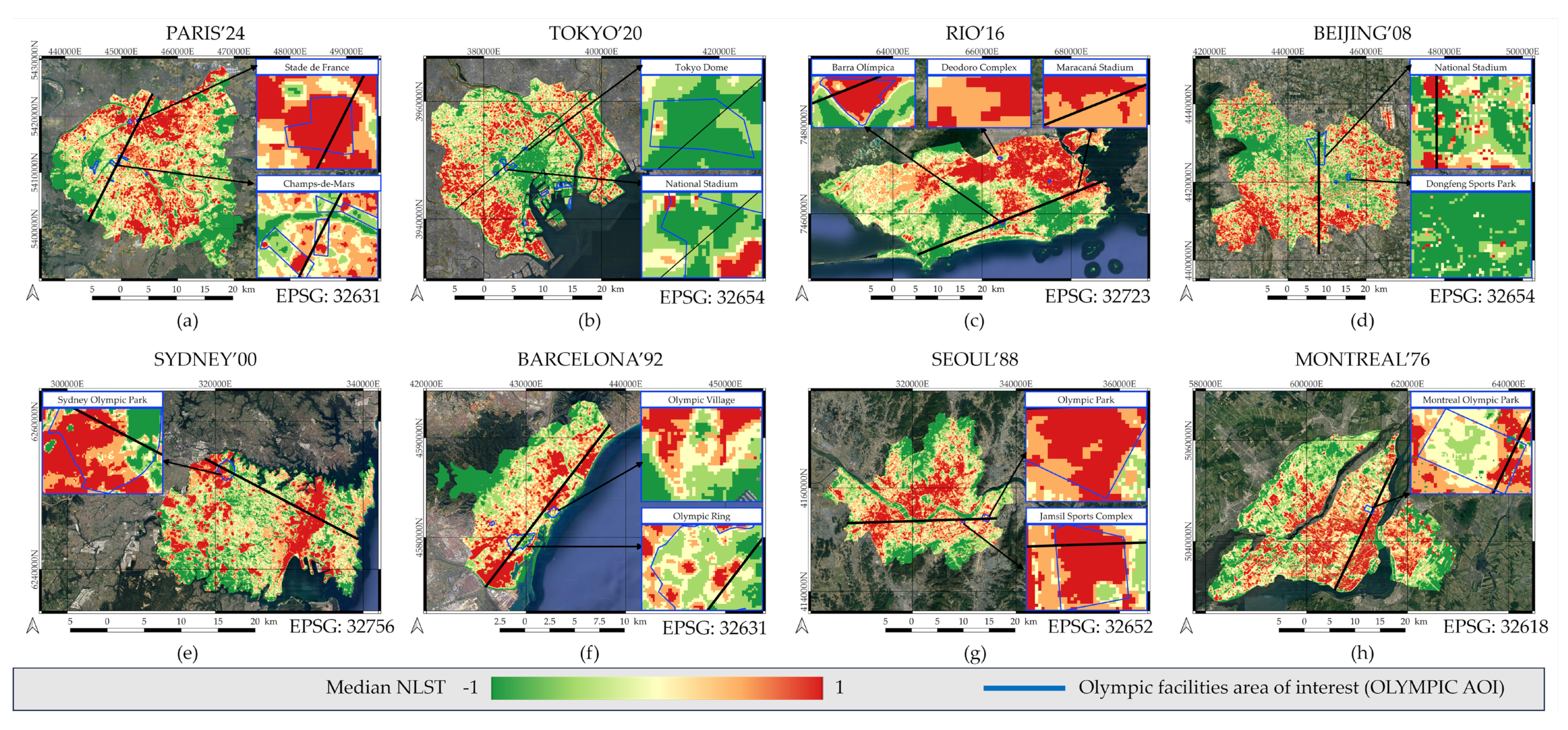
Figure 10.
Linear simple regressions relating the LST and the NLST pixels overlapped by the thermal transect defined in each city. The LST(K) and the NLST, are expected to perfectly correlate in a simple linear regression because they are simply converted using the scaling method (see 2.3.1 section).
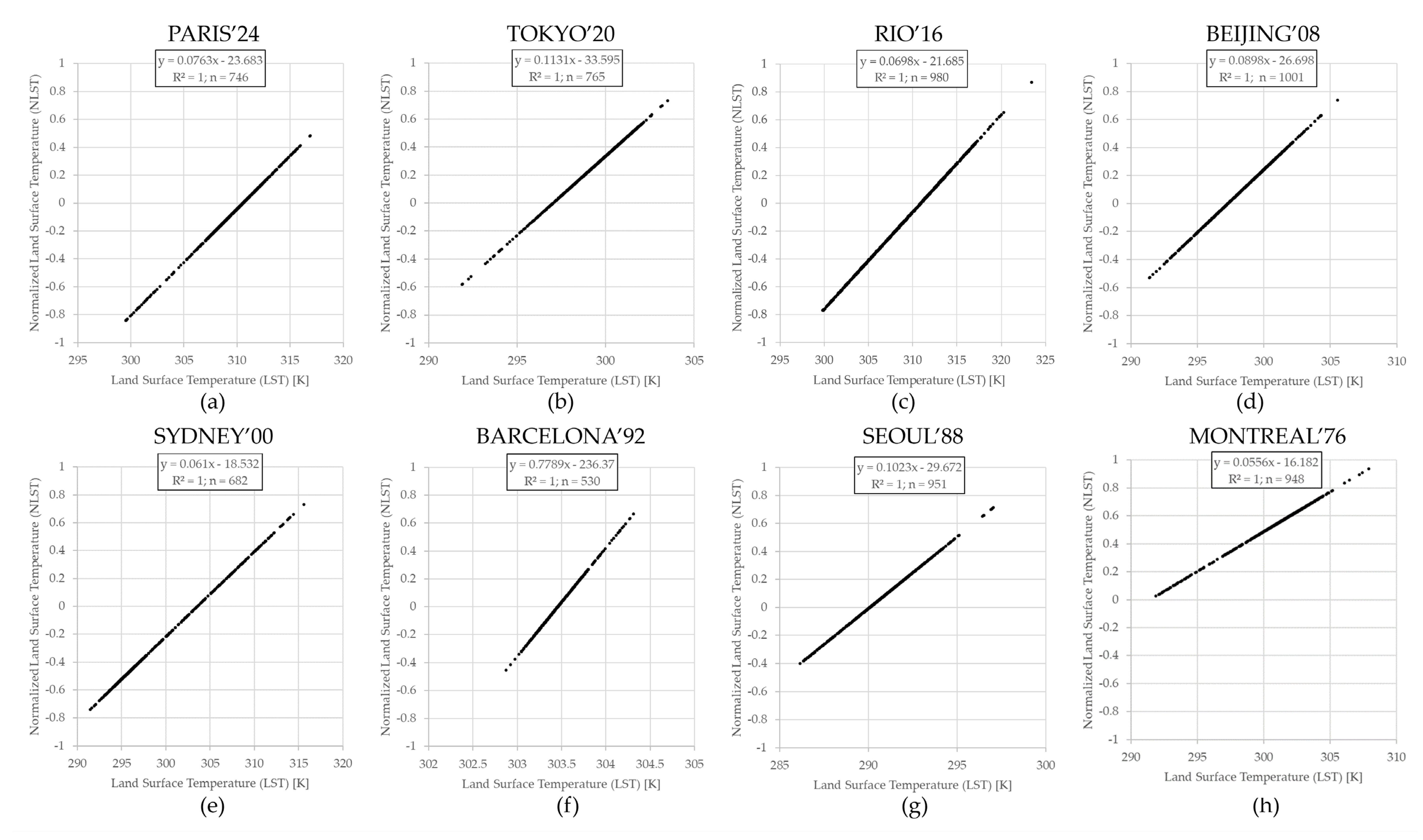
Table 1.
Summary of the Olympic cities analysed, its area, and Olympic facilities urban planning typology.
Table 1.
Summary of the Olympic cities analysed, its area, and Olympic facilities urban planning typology.
| Olympic game city |
Olympic year |
AOI urban area (km2) |
Olympic urban planning |
|---|---|---|---|
| Paris’24 | 2024 | 760 | Phase V / Cluster |
| Tokyo’20 | 2021 | 633 | Phase V / Polycentric |
| Rio’16 | 2016 | 1203 | Phase V / Periphery |
| London’12 | 2012 | 1568 | Phase V / Monocentric |
| Beijing’08 | 2008 | 1369 | Phase V / Polycentric |
| Athens’04 | 2004 | 274 | Phase IV / Periphery |
| Sydney’00 | 2000 | 392 | Phase IV / Periphery |
| Atlanta’96 | 1996 | 351 | Phase IV / Monocentric |
| Barcelona’92 | 1992 | 146 | Phase IV / Cluster |
| Seoul’88 | 1988 | 605 | Phase III / Monocentric |
| Los Angeles’84 | 1984 | 3721 | Phase III / Cluster |
| Moscow’80 | 1980 | 1053 | Phase III / Polycentric |
| Montreal’76 | 1976 | 894 | Phase III / Monocentric |
| Munich’72 | 1972 | 310 | Phase III / Monocentric |
Table 3.
Summary of each Olympic game city studied, the satellite that provided the imagery (Collection 2 Tier 1 Level 2), the path and row tile filtered, and the time interval of search. Also, only were selected images with less than a 5% of cloud cover over land. All this filtering resulted on a number of images from which it was calculated a synthetic image with the median value.
| Olympic game | Satellite | WRS2 Path-Row | Start date | End date | N images |
|---|---|---|---|---|---|
| Paris’24 | L8 and L9 | 199-26 | 01/01/2023 | 31/07/2024 | 10 |
| Tokyo’20 | L8 and L9 | 107-35 | 01/01/2020 | 31/12/2024 | 7 |
| Rio’16 | L8 | 217-76 | 01/01/2016 | 31/12/2020 | 17 |
| London’12 | L8 | 201-24 | 11/04/2013 | 31/12/2016 | 5 |
| Beijing’08 | L5 | 123-32 | 01/01/2008 | 31/12/2012 | 19 |
| Athens’04 | L5 | 183-34 | 01/01/2004 | 31/12/2008 | 26 |
| Sydney’00 | L5 and L7 | 089-84 | 01/01/2000 | 31/12/2004 | 30 |
| Atlanta’96 | L5 | 019-37 | 01/01/1996 | 31/12/2000 | 30 |
| Barcelona’92 | L5 | 197-31 | 01/01/1992 | 31/12/1996 | 17 |
| Seoul’88 | L4 and L5 | 116-34 | 01/01/1988 | 31/12/1992 | 21 |
| Los Angeles’84 | L4 and L5 | 041-36 & 37 | 01/01/1984 | 31/12/1988 | 41 |
| Moscow’80 | L4 and L5 | 178-21 | 16/07/1982 | 16/07/1987 | 5 |
| Montreal’76 | L4 and L5 | 014-28 | 16/07/1982 | 16/07/1987 | 12 |
| Munich’72 | L4 and L5 | 193-26 & 27 | 16/07/1982 | 16/07/1987 | 10 |
Table 4.
Summary of centrality zonal statistics of some selected Olympic game city studied. Zonal statistics are essentially calculated from the intersection of the AOI polygon and the target raster pixels values that are within (Land Surface Temperature (LST), Normalized Land Surface Temperature (NLST), Normalized Difference Vegetation Index (NDVI) and Normalized Difference Built-Up Index (NDBI).
| LST(K) | NLST | NDVI | NDBI | Pixel count | ||||||||||
|---|---|---|---|---|---|---|---|---|---|---|---|---|---|---|
| Mean | Median | Std. Dev. | Mean | Median | Std. Dev. | Mean | Median | Std. Dev. | Mean | Median | Std. Dev. | |||
| Paris ’24 |
AOI City | 308.54 | 309.13 | 3.81 | –0.15 | –0.10 | 0.29 | 0.22 | 0.20 | 0.12 | –0.07 | –0.05 | 0.09 | 1285931 |
| AOI Olympic | 309.15 | 308.94 | 3.00 | –0.11 | –0.12 | 0.23 | 0.18 | 0.17 | 0.12 | –0.06 | –0.06 | 0.08 | 5955 | |
| Difference | –0.61 | 0.19 | 0.82 | –0.05 | 0.02 | 0.06 | 0.18 | 0.17 | 0.12 | –0.01 | 0.00 | 0.01 | 1279976 | |
| Tokyo ’20 |
AOI City | 303.79 | 304.56 | 2.81 | 0.24 | 0.30 | 0.26 | 0.09 | 0.08 | 0.07 | –0.02 | –0.01 | 0.04 | 867511 |
| AOI Olympic | 300.97 | 300.94 | 2.59 | –0.03 | –0.04 | 0.24 | 0.20 | 0.21 | 0.11 | –0.07 | –0.07 | 0.07 | 7776 | |
| Difference | 2.83 | 3.62 | 0.21 | 0.27 | 0.34 | 0.02 | –0.11 | –0.13 | –0.04 | 0.06 | 0.06 | –0.02 | 859735 | |
| Rio ’16 |
AOI City | 307.85 | 307.88 | 4.07 | –0.17 | –0.16 | 0.29 | 0.23 | 0.25 | 0.12 | –0.07 | –0.07 | 0.10 | 1446446 |
| AOI Olympic | 311.81 | 311.94 | 2.28 | 0.12 | 0.12 | 0.16 | 0.12 | 0.08 | 0.11 | –0.01 | 0.00 | 0.07 | 3154 | |
| Difference | –3.96 | –4.06 | 1.79 | –0.29 | –0.28 | 0.13 | 0.11 | 0.17 | 0.01 | –0.06 | –0.07 | 0.03 | 1443292 | |
| Beijing ’08 |
AOI City | 298.01 | 298.25 | 2.32 | 0.06 | 0.08 | 0.21 | 0.09 | 0.09 | 0.04 | 0.00 | 0.00 | 0.03 | 1988537 |
| AOI Olympic | 296.42 | 296.32 | 1.85 | –0.08 | –0.09 | 0.17 | 0.10 | 0.09 | 0.05 | –0.02 | –0.02 | 0.03 | 36896 | |
| Difference | 1.60 | 1.93 | 0.47 | 0.14 | 0.17 | 0.04 | 0.00 | –0.01 | 0.00 | 0.02 | 0.02 | 0.01 | 1951641 | |
| Sydney ’00 |
AOI City | 296.39 | 295.62 | 3.38 | –0.47 | –0.52 | 0.22 | 0.15 | 0.15 | 0.08 | –0.02 | –0.02 | 0.06 | 525933 |
| AOI Olympic | 296.37 | 296.14 | 3.76 | –0.47 | –0.49 | 0.24 | 0.15 | 0.16 | 0.09 | –0.05 | –0.04 | 0.07 | 5895 | |
| Difference | 0.02 | –0.52 | –0.38 | 0.00 | –0.03 | –0.02 | 0.00 | –0.01 | –0.01 | 0.03 | 0.02 | –0.02 | 520038 | |
| Barcelona ’92 |
AOI City | 303.85 | 304.44 | 3.97 | –0.02 | 0.02 | 0.30 | 0.11 | 0.08 | 0.07 | 0.00 | 0.01 | 0.06 | 217207 |
| AOI Olympic | 303.14 | 303.09 | 1.82 | –0.07 | –0.08 | 0.14 | 0.15 | 0.16 | 0.06 | –0.04 | –0.04 | 0.05 | 4474 | |
| Difference | 0.71 | 1.34 | 2.15 | 0.05 | 0.10 | 0.16 | –0.04 | –0.07 | 0.01 | 0.04 | 0.05 | 0.01 | 212733 | |
| Seoul ’88 |
AOI City | 290.35 | 290.69 | 2.46 | –0.03 | 0.01 | 0.24 | 0.08 | 0.06 | 0.05 | 0.00 | 0.00 | 0.03 | 850246 |
| AOI Olympic | 292.40 | 292.28 | 1.43 | 0.17 | 0.16 | 0.14 | 0.09 | 0.08 | 0.04 | 0.00 | 0.00 | 0.02 | 2970 | |
| Difference | –2.05 | –1.59 | 1.03 | –0.20 | –0.15 | 0.10 | –0.01 | –0.02 | 0.01 | 0.00 | 0.00 | 0.01 | 847276 | |
| Montreal ’76 |
AOI City | 298.62 | 299.38 | 3.91 | 0.41 | 0.45 | 0.22 | 0.22 | 0.22 | 0.12 | –0.08 | –0.07 | 0.07 | 1421374 |
| AOI Olympic | 299.11 | 298.44 | 2.52 | 0.44 | 0.40 | 0.14 | 0.27 | 0.32 | 0.13 | –0.10 | –0.12 | 0.06 | 2967 | |
| Difference | –0.49 | 0.93 | 1.39 | –0.03 | 0.04 | 0.08 | –0.05 | –0.10 | –0.01 | 0.02 | 0.05 | 0.00 | 1418407 | |
Disclaimer/Publisher’s Note: The statements, opinions and data contained in all publications are solely those of the individual author(s) and contributor(s) and not of MDPI and/or the editor(s). MDPI and/or the editor(s) disclaim responsibility for any injury to people or property resulting from any ideas, methods, instructions or products referred to in the content. |
© 2024 by the authors. Licensee MDPI, Basel, Switzerland. This article is an open access article distributed under the terms and conditions of the Creative Commons Attribution (CC BY) license (http://creativecommons.org/licenses/by/4.0/).
Copyright: This open access article is published under a Creative Commons CC BY 4.0 license, which permit the free download, distribution, and reuse, provided that the author and preprint are cited in any reuse.


