
Submitted:
23 July 2024
Posted:
24 July 2024
You are already at the latest version
Abstract
The symptoms of multiple sclerosis (MS) are determined by the location of demyelinating lesions in the white matter of the brain and spinal cord. Currently, magnetic resonance imaging (MRI) is the most common tool for diagnosing MS, understanding the course of the disease, and analyzing the effects of treatments. However, undesirable components may appear during the generation of MRI, such as noise or intensity variations. Mathematical morphology (MM) is a powerful image analysis technique that helps to filter the image and extract relevant structures. Granulometry is an image measurement tool of MM that determines the size distribution of objects in an image without explicitly segmenting each object. While, several methods have been proposed for the automatic segmentation of MS lesions in MRI, in some cases only simple data preprocessing, such as image resizing to standardize the input dimensions, has been performed before the algorithm training. Therefore, this paper proposes an MRI preprocessing algorithm performing elementary morphological transformations in brain images of MS patients and healthy individuals to delete undesirable components and extract the relevant structures such as MS lesions. Also, the algorithm computes the granulometry in MRI to describe the size qualities of lesions and trains two artificial neural networks (ANN) to predict MS diagnosis. The computing of differences in granulometry measurements of an image with MS lesions and a reference image (without lesions) can determine the size characterization of the lesions. Then, the ANNs were evaluated with the validation set and the performance results (test accuracy = 0.9753, and cross-entropy loss = 0.0247) show the proposed algorithm can support the decision of specialists for diagnosing MS and estimating the disease progress, based on granulometry values.
Keywords:
Magnetic Resonance Imaging
; Multiple Sclerosis
; Mathematical Morphology
; Granulometry
; Artificial Neural Networks
1. Introduction
Multiple sclerosis (MS) is a chronic inflammatory disease of the central nervous system (CNS), characterized pathologically by demyelination and clinically by episodes of neurological dysfunction disseminated in space and time, which produces a wide variety of symptoms such as alteration of the sensitivity [1]. Symptoms are determined by the location of demyelinating lesions along the CNS [2]. Initially, MS pathology was defined as an inflammatory process associated with focal plaques of primary demyelination in the white matter of the brain and spinal cord [3]. A reliable and accurate diagnosis of MS is necessary to introduce early treatments for the disease. Disease-modifying drug therapies help to control symptoms and prevent progression [4,5]. Currently, magnetic resonance imaging (MRI) is the most common tool for diagnosing MS, understanding the course of the disease, and analyzing the effects of treatments [6,7].
MRI is a non-invasive method of obtaining detailed images of the internal structure of the body, such as organs and tissues. MRI uses radiofrequency (RF) radiation in the presence of controlled magnetic fields to generate cross-sectional images of the body. MRI is obtained by placing the patient inside a large magnet, which induces a relatively strong external magnetic field. This causes the cores of the body atoms to align with the magnetic field and then the RF signal is applied. The energy released from the body is detected and used to create the MRI by computer [8]. As with any other data acquisition system, in the generation of MRI, there may be a component not correlated with the desired signal, known as noise or random signal. This noise signal is generally caused by spontaneous fluctuations such as the thermal movement of free electrons within real or equivalent electrical components [9]. The signal-to-noise ratio (SNR) is essential for evaluating image quality and determining the use of image processing techniques such as noise removal [10]. On the other hand, MS diagnosis using MRI requires a long time due to the large number of images to be labeled (T1-weighted, T2-weighted, and fluid-attenuated inversion recovery (FLAIR) MRI), so manual diagnostic is susceptible to errors. Also, during the scan the Ghosting effect can happen, which is caused by objects in movement [11]. This can affect image quality and make it difficult to identify areas of CNS injury. Therefore, it is necessary to implement alternative methods of MRI automatic processing to remove noise and other undesirable components.
Most image processing applications require extensive analysis of objects within an image. Segmentation is to divide an image into regions of interest according to their features such as grayscale, color, spatial texture, and geometric shapes [12]. The most common form of segmentation is binary, where each pixel is classified as belonging to the foreground or background. One of the most useful methods for segmenting images is thresholding, which includes choosing an intensity value and then classifying pixels below this value as false and pixels above it as true [13]. On the other hand, mathematical morphology (MM) is a classic image analysis technique that helps to filter the image and extract relevant structures. Granulometry is an MM image measurement tool that determines the size distribution of objects in an image without explicitly segmenting each object [14]. So far, various learning models have been proposed for automatic segmentation of MS lesions in MRI, such as computational algorithms based on convolutional neural networks (CNN) [15]. Ghosh et al. [16] proposed four convolutional encoder networks (CENs) with different network architectures (U-Net, U-Net++, Linknet, and Feature Pyramid Network) to determine the optimal MRI sequence to reduce automatic segmentation times in MS lesions detection. La Rosa et al. [17] proposed a generative adversarial network (GAN) that retrospectively generates realistic magnetization prepared 2 rapid acquisition gradient echoes (MP2RAGE) uniform images (UNI) from MPRAGE images to improve automatic segmentation of MS lesions and tissues. Bandyopadhyay et al. [18] implemented a multilevel thresholding method using evolutionary metaheuristics. The proposal incorporates the concept of altruism into the Harris Hawks Optimization (HHO) algorithm to improve its exploitation capabilities. Macin et al. [19] developed a machine learning (ML) model for the MS diagnosis using brain MRI (axial and sagittal). Features were generated with a fixed-size patch-based (exemplar) feature extraction based on local phase quantization (LPQ). The resulting exemplar multiple parameters LPQ (ExMPLPQ) features were concatenated to form a final feature vector. De Oliveira et al. [20] proposed a deep learning (DL) technique for volumetric quantification of lesions in MRI of MS patients using automatic brain and lesion segmentation by two CNNs. The first CNN was used to perform brain extraction, and the second was for lesion segmentation. Acar et al. [21] proposed a CNN model for identifying MS lesions in brain FLAIR MRI. Hashemi et al. [22] implemented a method to segment MS lesions on FLAIR and T2 MRI using a modified U-Net and modified attention U-Net. Wang et al. [23] proposed a complete CNN U-Net for automatic segmentation of MRI, based on spine features and the contrast between gray levels of intervertebral discs and vertebrae. Rondinella et al. [24] implemented a model that includes a U-Net architecture augmented with a long short-term memory (LSTM) convolutional layer and an attention mechanism, capable of segmenting and quantifying MS lesions detected in MRI. Bose et al. [25] implemented a refined version of the fuzzy c-means (FCM) type 2 technique (EMT2FCM) to isolate diverse tissues in brain MRI, achieved through an improved entropy-based membership function.
While several methods have been proposed for the automatic segmentation of MS lesions in MRI, in some cases only simple data preprocessing, such as image resizing to standardize the input dimensions, has been performed before the algorithm training. Therefore, this paper proposes an alternative MRI preprocessing algorithm that includes two stages:
- Perform morphological opening transformations on brain MRI (MS patients and healthy individuals diagnosed by medical experts), to delete noise and other undesirable components. Also, to compute the granulometry of objects in MRI to characterize the demyelination lesions in the brain white matter caused by MS, and use the resulting data for training two artificial neural networks (ANN) models to predict the MS diagnosis.
- Perform morphological closing transformations on brain MRI (MS patients), to create a reference image (without lesions) and compute the granulometry of objects of an image with lesions and the reference image to be compared. Then, to determine the size of the MS lesions by calculating the differences in granulometry measurements. These measurements could support the decision of specialists to estimate the course or progress of the disease.
2. Materials and Methods
2.1. Database
The analyzed database is the same as [19], and it can be downloaded at: https://www.kaggle.com/datasets/buraktaci/multiple-sclerosis (accessed on 20 October 2023). The acquired dataset includes 200 brain FLAIR MRI (100 axial and 100 sagittal) from MS patients and healthy individuals, who attended the Ozal University Faculty of Medicine in 2021. Medical experts analyzed the sections of axial and sagittal images of MS patients with identifiable MS lesions which were assigned to the MS class, and image sections of healthy individuals with normal appearance, without white matter lesions, and were assigned to the healthy class.
2.2. Mathematical Morphology
MM is a powerful image analysis technique based on set theory, integral geometry, and lattice algebra. The target of morphological operators is to extract relevant structures from an image. It is achieved by testing the image with another set of known shapes called a structuring element (SE). The fundamental morphological operators need the definition of an origin for each SE. This origin allows the positioning of the SE at a given point or pixel: an SE at point x means its origin matches x. The elementary planar isotropic SEs are represented in Figure 1 for octagonal and disk graphs. The pixels that match with the elemental planar SE centered on a given pixel p correspond to the neighbors of p in the graph G plus the pixel itself p, . The shape and size of the SE are chosen according to the geometric properties of the relevant and irrelevant structures in the image. Irrelevant structures refer to noise or objects to be deleted [26].
2.3. Geodesic Transformations
Some morphological transformations include combinations of an input image with specific SEs. The geodesic transformations approach regards two input images. Initially, a morphological transformation is applied to the first image and then forced to remain either above or below the second image. In this case, morphological transformations are limited to elementary erosions and dilations. In practice, geodetic transformations are iterated until stability [27].
A geodesic dilation involves two images, a marker image and a mask image. By definition, both images must have the same domain and the mask image must be greater than or equal to the marker image. First, the marker image is dilated by the elemental isotropic SE. Then, the resulting dilated image is forced to remain below the mask image. Therefore, the mask image acts as a limit to the spread of the marker image dilation. Let f be the marker image and g be the mask image ( and ). The geodesic dilation of size 1 of the marker image f concerning the mask image g is denoted by Equation 1 and it is defined as the minimum point between the mask image and the elemental dilation of the marker image. The geodesic dilation of a binary image is shown in Figure 2.
Geodesic erosion is the double transformation of geodesic dilation concerning the complementation of sets:
where and is the elemental erosion. First, the marker image is eroded and then the maximum point is computed with the mask image. Figure 3 shows an example of geodesic erosion. Here, the mask image acts as a limit for the marker image reduction.
2.4. Morphological Reconstruction
In practice, geodesic transformations of a given size are rarely used. However, when they are iterated until stability, very efficient morphological reconstruction algorithms can be created. Geodesic transformations of bounded images always converge after a finite time of iterations (i.e., until the mask image completely obstructs the propagation or reduction of the marker image). The morphological reconstruction of a mask image g from a marker image f is based on this principle. Geodesic transformations by reconstruction allow the deletion of some undesired components without considerably affecting the remaining structures [27].
Like geodesic dilations and erosions, the iteration of the autodual geodesic transformation v always achieves stability for a definition domain of a bounded image. The corresponding transformation is known as the self-dual reconstruction of a mask image g from a marker image f and it is defined as:
where i is such . Figure 4 displays self-dual reconstruction. In practice, self-dual reconstruction can be obtained by computing erosion and dilation reconstruction in parallel, the output at a given pixel x alternating between erosion and dilation reconstruction depending on whether is above or below :
2.4.1. Opening and Closing by Reconstruction
For morphological reconstruction, the erosion and dilation of size 1 are iterated until stability is achieved. The geodesic dilation and the geodesic erosion of size 1 are given by with , and with , respectively. When the function g is equal to the morphological erosion or dilation of the original function, the opening by reconstruction is given by:
or the closing by reconstruction is given by:
where B represents the SE and is a size parameter. For this research, a disk-shaped SE with radius () is chosen. For example, a disk of radius represents a disk of 9x9 pixels, therefore, 9 neighbors are analyzed. So, an SE of size n consists of a disk of pixels.
2.5. Image Measurements
Image measurements aim to characterize objects in an image by computing some numerical values. For a given criterion, the measurement is discriminant if the obtained values for objects satisfying this criterion differ from those for all other objects. MM provides various image measurement tools such as pattern spectrum or granulometry, direction analysis, texture analysis, shape description, etc. These measures define a vector of features that can be used as input for a statistical analysis or classification method [26].
Granulometry determines the size distribution of objects in an image without explicitly segmenting (detecting) each object, and it is used in some areas to describe the features of the size and shape of individual granules within an object [28]. The formal definition of this concept is presented below.
Granulometry.- Let to be a transformations family depending of a unique positive parameter . This family comprises a granulometry if and only if the following properties are fulfilled: (i) positive is increasing, (ii) positive, is antiextensional, (iii) and positives, .
In particular, the family of morphological openings and closings for the numerical instance , with satisfy the previous definition.
The granulometric measurement associated with the clear regions is denoted as , and it is computed by:
where refers to the total number of pixels in an image. The granulometric measurement associated with the dark regions is denoted as and it is calculated by:
2.6. Proposed Algorithm
This paper proposes an alternative MRI preprocessing algorithm including elementary morphological transformations and granulometry computing to characterize MS lesions without affecting the image original dimensions of the image. The proposed algorithm is described below and it is divided into two stages.
-
Perform opening morphological transformations on brain images of MS patients and healthy individuals (axial and sagittal MRI), compute the granulometry of objects (Equation 7), and use the resulting data to train two ANN models, applying the following steps:
- Read the original color image (.png) and convert it to grayscale (e.g. uint8 array 569x1158x3 → uint8 array 569x1158).
- Perform a morphological opening transformation on the image in grayscale (mask image) to create a marker image using a SE. This operation consists of an erosion followed by a dilation using the same SE. The created SE is disk-shaped with radius r, which matches the geometric properties of the relevant structures of a brain image.
- Perform an opening by reconstruction transformation on the mask image (Equation 5), using the marker image to identify high-intensity objects in the mask image.
- Adjust the intensity values of the opened image by reconstruction, which increases the contrast of the output image, to extract relevant structures (MS lesions).
- Compute the granulometry of objects of the opened image by reconstruction for different radius values () of the SE.
- Enter the granulometry measurements of each sample into two arrays (axial and sagittal) of dimension: 100 samples x 15 features (radius values) = 1500 samples for each array.
- Train two ANN models with the granulometry measurements, using MATLAB R2023a software, to make predictions of MS diagnosis.
-
Perform closing morphological transformations on brain images of MS patients (axial and sagittal MRI) to determine the size of the MS lesions, applying the following steps:
- Subtract the lesion areas from the mask image (original image) to acquire a brain image without lesions (with holes).
- Perform a morphological closing transformation on the resulting image (previous step) using a disk-shaped SE with radius r to create a marker image. This operation consists of a dilation followed by erosion using the same SE.
- Perform a closing by reconstruction transformation on the marker image (Equation 6), using the mask image to fill the holes and create a reference image (without lesions), for making comparisons with the mask image (with lesions).
- Compute the granulometry of objects of the mask image and the reference image for different values of radius () of the SE.
- Determine the size of MS lesions by computing the differences in granulometry measurements of the mask image and the reference image to support the decision of specialists in estimating the disease progress.
Figure 5 and Figure 6 describe the two-stage procedure of the proposed algorithm. Table 1 and Table 2 present the implemented pseudocode of the preprocessing algorithm.
2.6.1. Artificial Neural Network
The ANN structure consists of an input layer of neurons that receive the sample inputs , one or more hidden layers of neurons that convert the values from the previous layer into a weighted linear sum, , followed by a not linear activation function used to learn the weights. Then the output layer predicts the class label of the samples [29]. During the learning stage, ANN compares the true class labels with the continuous output values of the nonlinear activation function to compute the classification loss and update the weights.
The dataset is randomly divided into training (80%) and test (20%) sets to validate the ANN models. Then, the test accuracy, the dice similarity coefficient (DSC), true positive rate (TPR) or sensitivity, and true negative rate (TNR) or specificity were computed with the validation dataset to evaluate the performance of prediction models [30,31,32]. DSC is given by,
where TP, TN, FP, and FN represent true positives, true negatives, false positives, and false negatives, respectively. Also, the cross-entropy loss is calculated with different regularization strength values (lambda hyperparameter) to train the ANNs. The weighted cross-entropy loss is,
where the weights are normalized to sum to n instead 1. The test accuracy is calculated by . The lambda value is adjusted to minimize the loss function. Table 3 describes the configured hyperparameters for the ANNs training.
3. Results
The proposed MRI preprocessing algorithm was implemented on 100 MS sample images (axial) and 100 healthy sample images (sagittal). Also, granulometry was calculated to acquire relevant information about some structures in the brain images. In particular, the morphological opening transformation was used as a filter that satisfies the definition of granulometry and mainly affects the clear regions directly associated with MS lesions.
3.1. Algorithm (Stage 1)
In the first stage, the preprocessing algorithm was implemented in all MS and healthy images (axial and sagittal MRI). Figure 7 and Figure 8 describe the obtained results of the applied opening morphological transformations.
Then, granulometry of objects was computed in all MRI samples for an SE of different radius values (). Figure 9 compares the granulometry measurements results in brain images of two MS patients (axial and sagittal) and two healthy individuals (axial and sagittal) with similar dimensions respectively (569x1158 pixels).
After granulometry was computed, the resulting data were entered into two arrays (100x15 samples) to train the ANNs. Table 4 and Table 5 present granulometry values of some samples (axial and sagittal). Also, Figure 10 displays the values of the sum of granulometry of 80 MRI samples (axial and sagittal).
Then, the performance metrics (DSC, sensitivity, and specificity) were computed using the confusion matrix results to evaluate the ANN models. Figure 11 shows the counting of predictions of the ANNs.
Also, the cross-entropy loss was calculated with different regularization strength values, the corresponding results are displayed in Figure 12. So, the ANNs were trained using the best lambda regularization strengths. Figure 13 displays the loss function behavior throughout different iterations.
Table 6 compares the performance metrics results of the implemented ANN models.
3.2. Algorithm (Stage 2)
At the second stage of the implemented algorithm, the MS lesion areas (acquired at the intensity adjustment step) were subtracted from the mask image (original image), and the morphological closing transformation of the resulting image (with lesion holes) was computed. Then, the image was closed by reconstruction to fill the holes, and a reference image (without lesions) was created to be compared with the mask image (with lesions). The previous procedure was applied to two MS sample images (axial and sagittal), and the results are displayed in Figure 14 and Figure 15.
Finally, the granulometry of objects of the mask image and the reference image were computed. Figure 16 and Figure 17 show the granulometry results of two MS sample images (axial and sagittal). To determine the size of the MS lesions, the difference of granulometry measurements at each data point was calculated, with a disk-shaped SE for different radius values ().
4. Discussion
Segmentation is useful for analyzing and identifying damaged tissues or other abnormalities in MRI and for different tasks such as disease diagnosis [12]. Although several computational models have been proposed for the automatic segmentation of MS lesions in MRI, in some cases only simple data preprocessing (image resizing to standardize the input dimensions) has been performed before the algorithm training [14,16,17,18]. Therefore, this paper proposes an MRI preprocessing algorithm based on elementary morphological transformations and granulometry computing. The algorithm helps filter the image by eliminating undesired components without affecting its original dimensions. Also, it improves the characterization of MS lesions by extracting only the relevant structures.
At the first stage of the proposed algorithm, morphological opening transformations were performed on the brain images to identify high-intensity objects (clear objects can be associated with MS lesions), followed by intensity adjustment to increase the contrast and extract the relevant structures. Also, the granulometry of objects in the preprocessed images was computed. The granulometry results in Figure 9 show that the intensity values in MS brains are higher than in healthy brains, so these measurements are directly associated with the lesions. Then, the granulometry values were used to train two ANN models to predict MS diagnosis. The performance metrics results in Table 6 prove granulometry measurements work as efficient predictors to train ANN models. In this way, this algorithm can support the decision of specialists to diagnose MS based on granulometry computing. Also, the loss function behavior in Figure 13 indicates it is not necessary to spend so much time tuning the hyperparameters of a learning model, only by adjusting the regularization strength hyperparameter (lambda) it is possible to minimize the loss. Table 7 compares the performance results of some studies in the analysis of MS lesions in MRI. A limitation of this paper was that some MRIs available in the analyzed database had different dimensions, so only 100 images of MS patients (axial and sagittal) and 100 images of healthy individuals (axial and sagittal) of dimension: 569x1158x3 pixels were chosen.
In the second stage of the implemented algorithm, morphological closing transformations were performed on brain MRI (MS patients), to create an image of a healthy brain approach (reference image). Then, the granulometry of objects of an image with MS lesions and the reference image was computed to determine the size of the lesions. The results in Figure 12 and Figure 13 show it is possible to estimate the size of MS lesions by calculating the difference of granulometry measurements at each data point. These measurements could support the decision of specialists to estimate the progress of the disease and possibly prescribe some specific treatment.
To validate the results of this paper, they were analyzed by a neurologist expert. So, he commented the characterization of the size of the lesions based on granulometry measurements could be useful to monitor a load of activity (new plaques in MS), monitor the progress of other demyelinating diseases such as Devic disease (at the spinal cord level), and monitor tumor growth of gliomas of low grade and even multiform glioblastoma (to evaluate the response to treatment: tumor reduction).
Conflicts of Interest
The authors declare no conflicts of interest.
Abbreviations
The following abbreviations are used in this manuscript:
| MS | Multiple sclerosis |
| MRI | Magnetic resonance imaging |
| MM | Mathematical morphology |
| ANN | Artificial neural network |
| CNS | Central nervous system |
| RF | Radiofrequency |
| SNR | Signal-to-noise ratio |
| FLAIR | Fluid-attenuated inversion recovery |
| CNN | Convolutional neural network |
| CEN | Convolutional encoder network |
| GAN | Generative adversarial network |
| MP2RAGE | Magnetization prepared 2 rapid acquisition gradient echoes |
| UNI | Uniform image |
| HHO | Harris hawks optimization |
| ML | Machine learning |
| LPQ | Local phase quantization |
| ExMPLPQ | Exemplar multiple parameters local phase quantization |
| LSTM | Long short-term memory |
| FCM | Fuzzy c-means |
| SE | Structuring element |
| DSC | Dice similarity coefficient |
| TPR | True positive rate |
| TNR | True negative rate |
References
- Fernández, O., Fernández, V., E., Guerrero, M. Esclerosis múltiple. Medicine, Programa de Formación Médica, 2015, 11(77), 4610-4621.
- Milo, R., & Miller, A. Revised diagnostic criteria of multiple sclerosis. Autoimmunity reviews, 2014, 13(4-5), 518-524. [CrossRef]
- Lassmann, H., Brück, W., Lucchinetti, C. F. The immunopathology of multiple sclerosis: an overview. Brain pathology, 2007, 17(2), 210-218. [CrossRef]
- Murray, T. J. Diagnosis and treatment of multiple sclerosis. Bmj, 2006, 332(7540), 525-527. [CrossRef]
- Hočevar, K., Ristić, S., Peterlin, B. Pharmacogenomics of multiple sclerosis: a systematic review. Frontiers in neurology, 2019, 10, 134. [CrossRef]
- Lladó, X., Oliver, A., Cabezas, M., Freixenet, J., Vilanova, J. C., Quiles, A., Rovira, À. Segmentation of multiple sclerosis lesions in brain MRI: a review of automated approaches. Information Sciences, 2012, 186(1), 164-185. [CrossRef]
- Wildner, P., Stasiołek, M., Matysiak, M. Differential diagnosis of multiple sclerosis and other inflammatory CNS diseases. Multiple sclerosis and related disorders, 2020, 37, 101452. [CrossRef]
- Katti, G., Ara, S. A., Shireen, A. Magnetic resonance imaging (MRI)–A review. International journal of dental clinics, 2011, 3(1), 65-70.
- Macovski, A. Noise in MRI. Magnetic resonance in medicine, 1996, 36(3), 494-497.
- Hendee, W. R., & Ritenour, E. R. Fundamentals of magnetic resonance. Medical imaging physics, 2002, NY: Wiley-Liss, 355-365.
- Uyttendaele, M., Eden, A., Skeliski, R. Eliminating ghosting and exposure artifacts in image mosaics. In Proceedings of the 2001 IEEE Computer Society Conference on Computer Vision and Pattern Recognition, 2001, 2, II-II.
- Liu, X., Song, L., Liu, S., Zhang, Y. A review of deep-learning-based medical image segmentation methods. Sustainability, 2021, 13(3), 1224. [CrossRef]
- Norouzi, A., Rahim, M. S. M., Altameem, A., Saba, T., Rad, A. E., Rehman, A., Uddin, M. Medical image segmentation methods, algorithms, and applications. IETE Technical Review, 2014, 31(3), 199–213. [CrossRef]
- de Arruda, A. L. C., Vital, D. A., Kitamura, F. C., Abdala, N., Moraes, M. C. Multiple sclerosis segmentation method in magnetic resonance imaging using fuzzy connectedness, binarization, mathematical morphology, and 3D reconstruction. Research on Biomedical Engineering, 2020, 36, 291-301. [CrossRef]
- Shen, D.; Wu, G.; Suk, H.I. Deep learning in medical image analysis. Annu. Rev. Biomed. Eng., 2017, 19, 221–248.
- Ghosh, S., Huo, M., Shawkat, M. S. A., McCalla, S. Using convolutional encoder networks to determine the optimal magnetic resonance image for the automatic segmentation of multiple sclerosis. Applied Sciences, 2021, 11(18), 8335. [CrossRef]
- La Rosa, F., Yu, T., Barquero, G., Thiran, J. P., Granziera, C., Cuadra, M. B. MPRAGE to MP2RAGE UNI translation via generative adversarial network improves the automatic tissue and lesion segmentation in multiple sclerosis patients. Computers in Biology and Medicine, 2021, 132, 104297. [CrossRef]
- Bandyopadhyay, R., Kundu, R., Oliva, D., Sarkar, R. Segmentation of brain MRI using an altruistic Harris Hawks’ Optimization algorithm. Knowledge-Based Systems, 2021, 232, 107468. [CrossRef]
- Macin, G., Tasci, B., Tasci, I., Faust, O., Barua, P. D., Dogan, S., Acharya, U. R. An accurate multiple sclerosis detection model based on exemplar multiple parameters local phase quantization: ExMPLPQ. Applied Sciences, 2022, 12(10), 4920. [CrossRef]
- de Oliveira, M., Piacenti-Silva, M., da Rocha, F. C. G., Santos, J. M., Cardoso, J. D. S., Lisboa-Filho, P. N. Lesion volume quantification using two convolutional neural networks in MRIs of multiple sclerosis patients. Diagnostics, 2022, 12(2), 230. [CrossRef]
- Acar, Z. Y., Başçiftçi, F., Ekmekci, A. H. Convolutional Neural Network model for identifying Multiple Sclerosis on brain FLAIR MRI. Sustainable Computing: Informatics and Systems, 2022, 35, 100706. [CrossRef]
- Hashemi, M., Akhbari, M., Jutten, C. Delve into multiple sclerosis (MS) lesion exploration: a modified attention U-net for MS lesion segmentation in brain MRI. Computers in Biology and Medicine, 2022, 145, 105402. [CrossRef]
- Wang, Z., Xiao, P., Tan, H. Spinal magnetic resonance image segmentation based on U-net. Journal of Radiation Research and Applied Sciences, 2023, 16(3), 100627. [CrossRef]
- Rondinella, A., Crispino, E., Guarnera, F., Giudice, O., Ortis, A., Russo, G., Battiato, S. Boosting multiple sclerosis lesion segmentation through attention mechanism. Computers in Biology and Medicine, 2023, 161, 107021. [CrossRef]
- Bose, A., Maulik, U., Sarkar, A. An entropy-based membership approach on type-II fuzzy set (EMT2FCM) for biomedical image segmentation. Engineering Applications of Artificial Intelligence, 2024, 127, 107267. [CrossRef]
- Soille, P. Morphological image analysis: principles and applications. Berlin: Springer., 1999, 2(3), 170-171.
- Soille, P. Geodesic transformations. Morphological Image Analysis: Principles and Applications., 2004, Springer, 183-218.
- Santibáñez, J. D. M., Duarte, M. G., Retana, J. J. O., Campos, C. E. L. Segmentación y análisis granulométrico de sustancia blanca y gris en IRM para el estudio del estrabismo usando transformaciones morfológicas. Revista Mexicana de Ingeniería Biomédica., 2007, 28(2), 13-13.
- Casalino, G., Castellano, G., Consiglio, A., Nuzziello, N., Vessio, G. MicroRNA expression classification for pediatric multiple sclerosis identification. Journal of Ambient Intelligence and Humanized Computing, 2023, 14(12), 15851-15860. [CrossRef]
- Sudre, C.H.; Li, W.; Vercauteren, T.; Ourselin, S.; Cardoso, M.J. Generalised Dice Overlap as a Deep Learning Loss Function for Highly Unbalanced Segmentations. Springer International Publishing, 2017, 240-248. [CrossRef]
- Cardenas, C. E., McCarroll, R. E., Court, L. E., Elgohari, B. A., Elhalawani, H., Fuller, C. D., Aristophanous, M. (2018). Deep learning algorithm for auto-delineation of high-risk oropharyngeal clinical target volumes with built-in dice similarity coefficient parameter optimization function. International Journal of Radiation Oncology* Biology* Physics, 2018, 101(2), 468-478. [CrossRef]
- Goyal, M., Khanna, D., Rana, P. S., Khaibullin, T., Martynova, E., Rizvanov, A. A., ... & Baranwal, M. (2019). Computational intelligence technique for prediction of multiple sclerosis based on serum cytokines. Frontiers in neurology, 2019, 10, 781. [CrossRef]
Figure 1.
Elementary flat isotropic SE for octagon and disk graphs: (a) Diamond. (b) Octagon. (c) Disk. The origin of these SEs is at their center.
Figure 1.
Elementary flat isotropic SE for octagon and disk graphs: (a) Diamond. (b) Octagon. (c) Disk. The origin of these SEs is at their center.
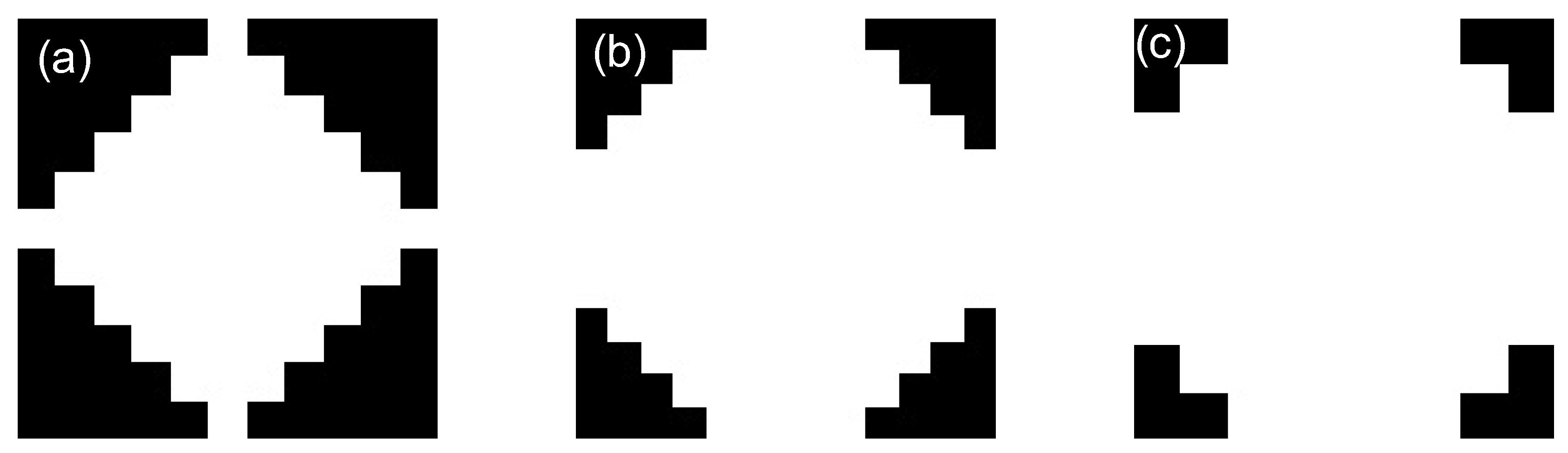
Figure 2.
Geodesic dilation of a binary image or set Y within a geodesic mask X. The marker set is first dilated by the elementary isotropic SE and then intersected with the geodesic mask: .
Figure 2.
Geodesic dilation of a binary image or set Y within a geodesic mask X. The marker set is first dilated by the elementary isotropic SE and then intersected with the geodesic mask: .
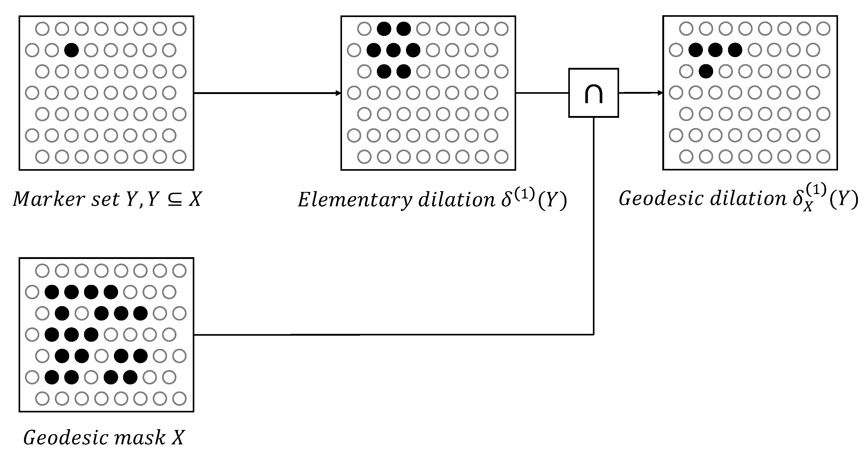
Figure 3.
Geodesic erosion of a 1-D marker signal f with respect to a mask signal g. Owing to the point-wise maximum operator, all pixels of the elementary erosion of f having values lower than g are set to the value of g.
Figure 3.
Geodesic erosion of a 1-D marker signal f with respect to a mask signal g. Owing to the point-wise maximum operator, all pixels of the elementary erosion of f having values lower than g are set to the value of g.
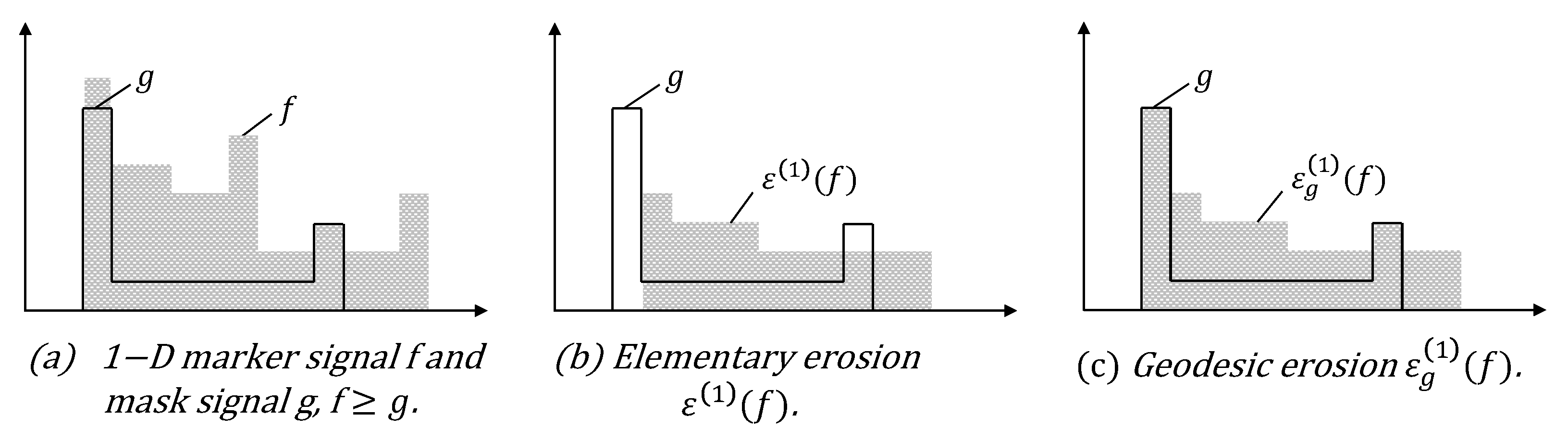
Figure 4.
Self-dual morphological reconstruction of a mask image g from a marker image f.
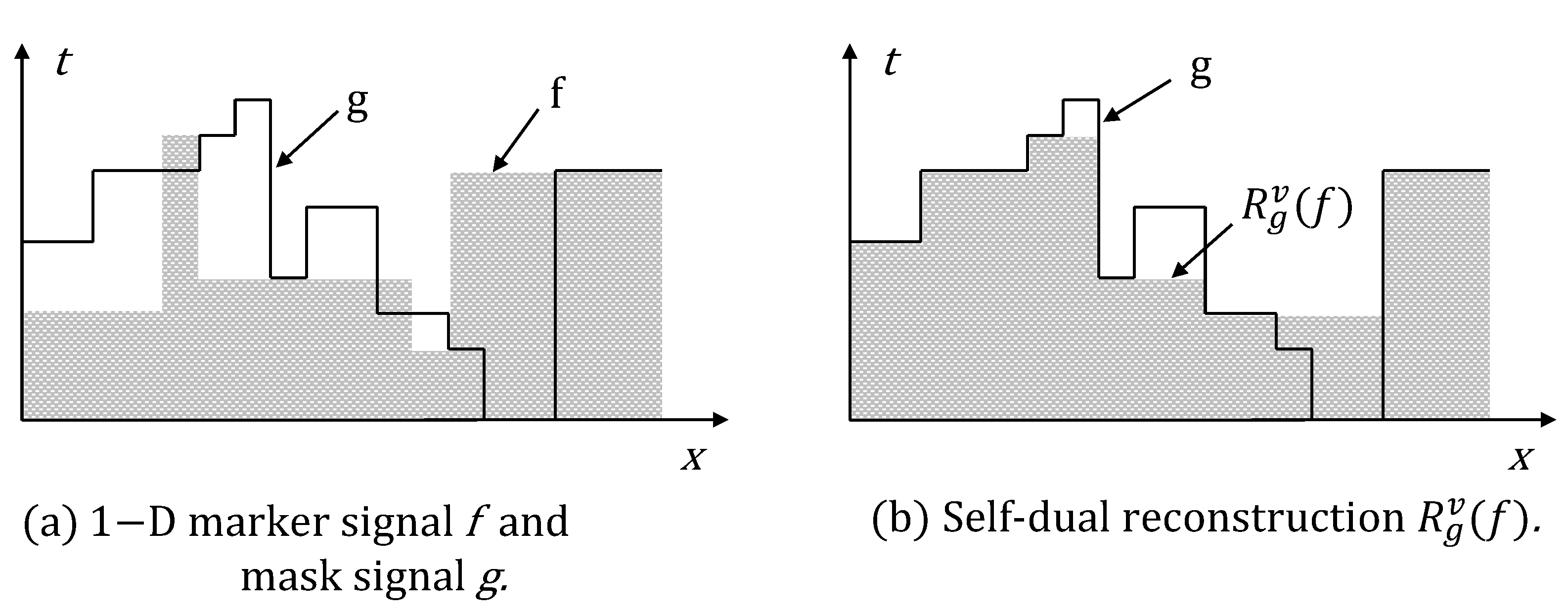
Figure 5.
First stage procedure of the proposed algorithm. Opening morphological transformations on MS and healthy brains and granulometry computing to predict MS diagnosis).
Figure 5.
First stage procedure of the proposed algorithm. Opening morphological transformations on MS and healthy brains and granulometry computing to predict MS diagnosis).
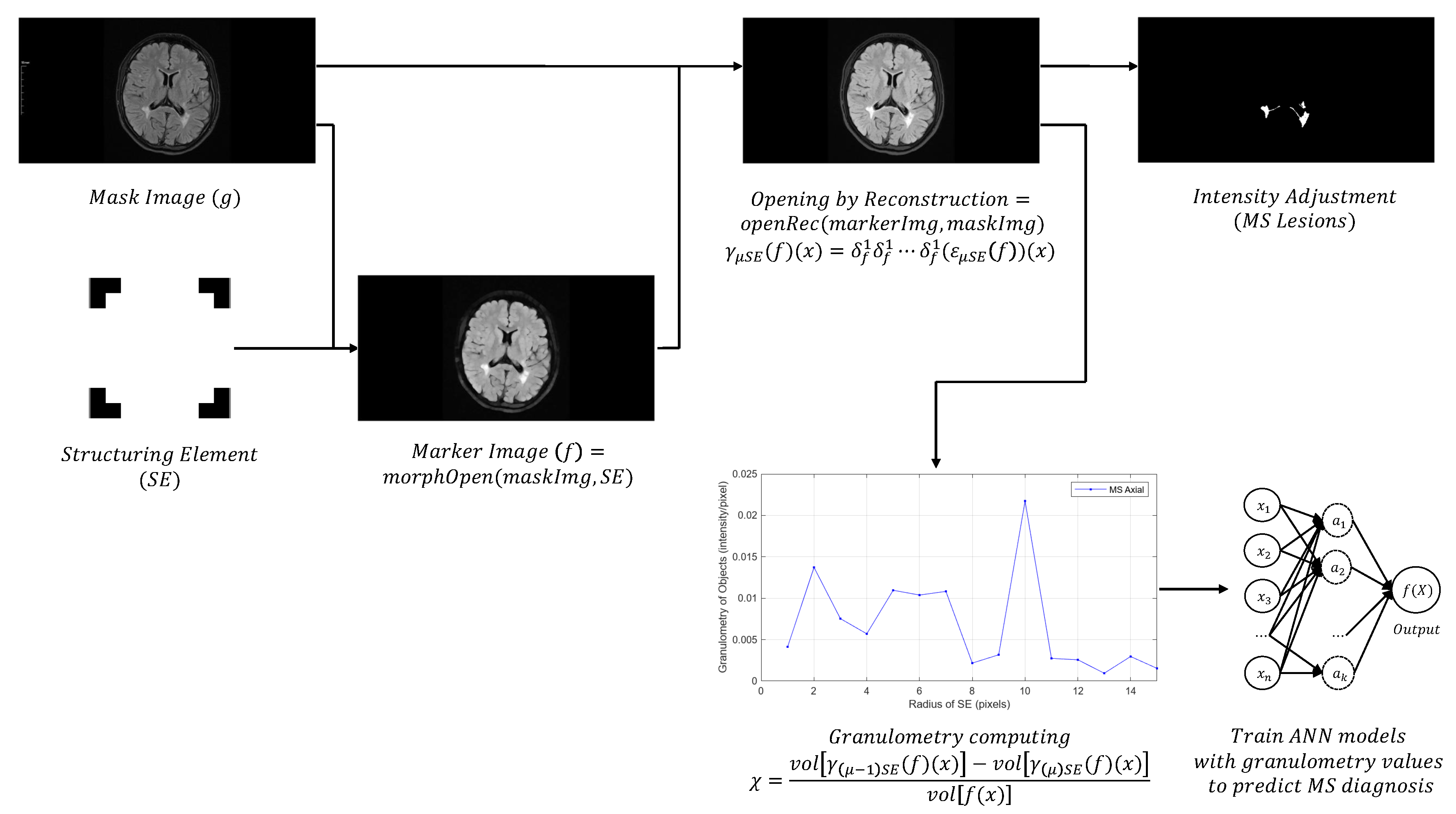
Figure 6.
Second stage procedure of the proposed algorithm. Closing morphological transformations on MS brains and granulometry computing to determine the MS lesions size for estimating the disease progress).
Figure 6.
Second stage procedure of the proposed algorithm. Closing morphological transformations on MS brains and granulometry computing to determine the MS lesions size for estimating the disease progress).
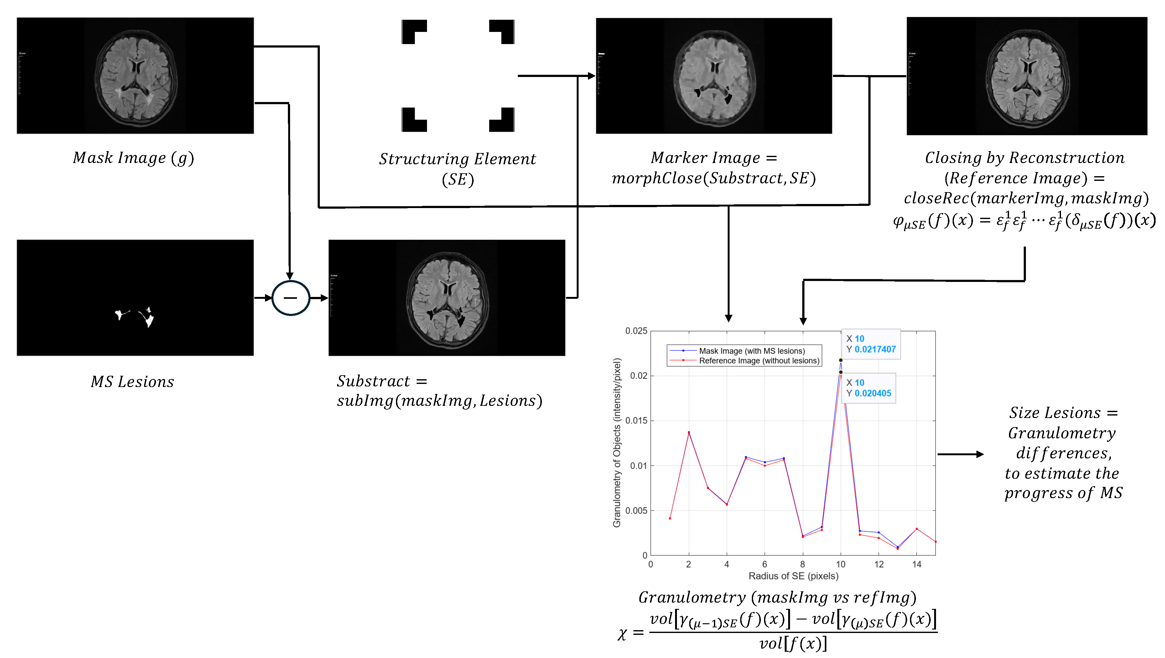
Figure 7.
Implementation of opening morphological transformations. (a) Mask image (MS axial). (b) Morphological opening. (c) Opening by reconstruction. (d) Intensity adjustment. One of the targets of the first stage was to highlight the lesion areas in MS samples (axial MRI), using a disk-shaped SE of radius r=5.
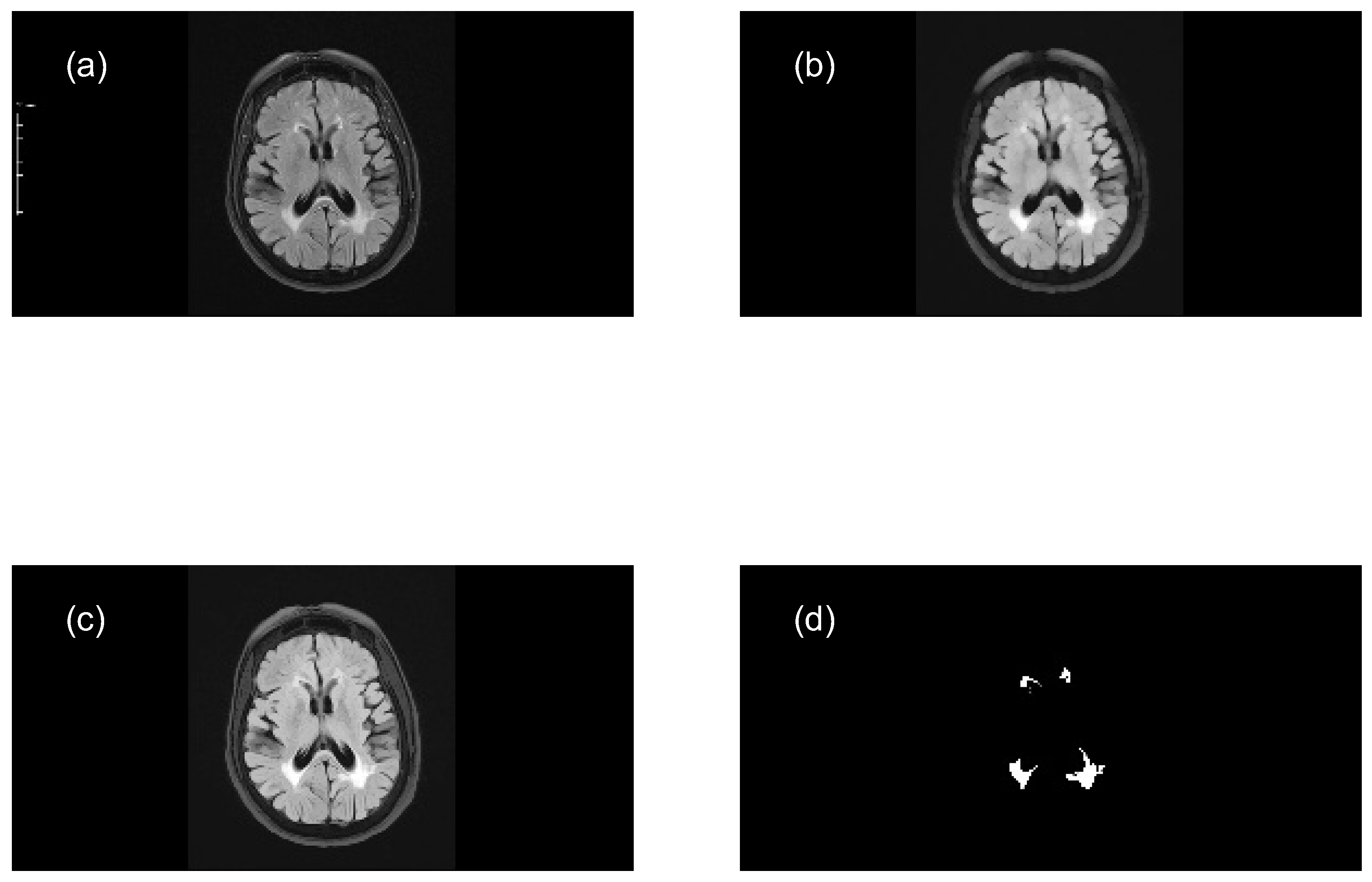
Figure 8.
Implementation of opening morphological transformations. a) Mask Image (MS sagittal). (b) Morphological opening. (c) Opening by reconstruction. (d) Intensity adjustment. One of the targets of the first stage was to highlight the lesion areas in MS samples (sagittal MRI), using a disk-shaped SE of radius r=5.
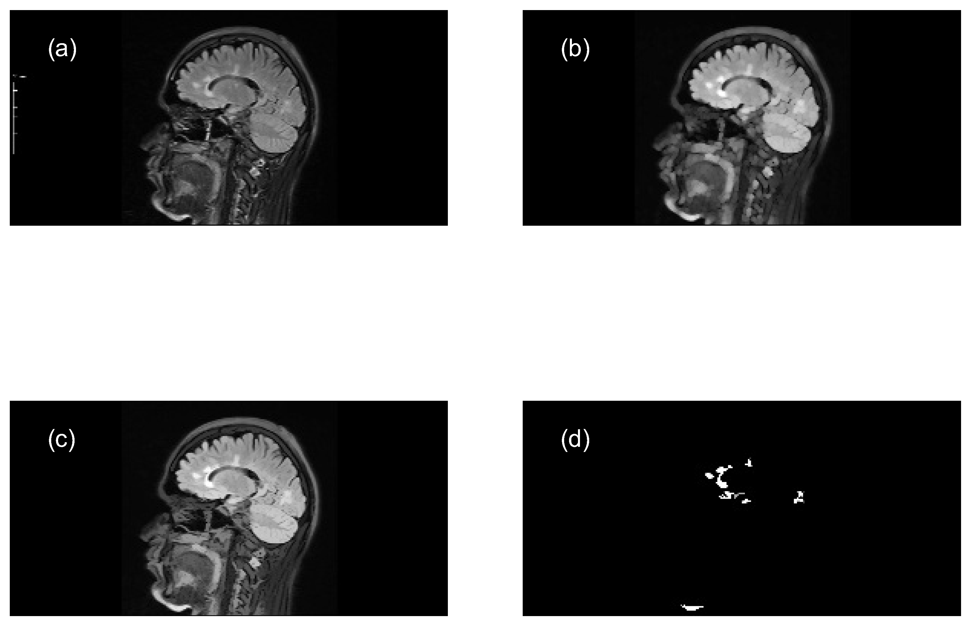
Figure 9.
Comparison of granulometry measurements in preprocessed brain images by the proposed algorithm (stage 1). (a) MS axial image (SumVolGranu=0.1011). (b) Healthy axial image (SumVolGranu=0.0786). (c) MS sagittal image (SumVolGranu=0.1389). (d) Healthy sagittal image (SumVolGranu=0.1079). The sum of intensity values of objects (sumVolGranu) in MS brains is higher than in healthy brains, due to the presence of lesion regions.
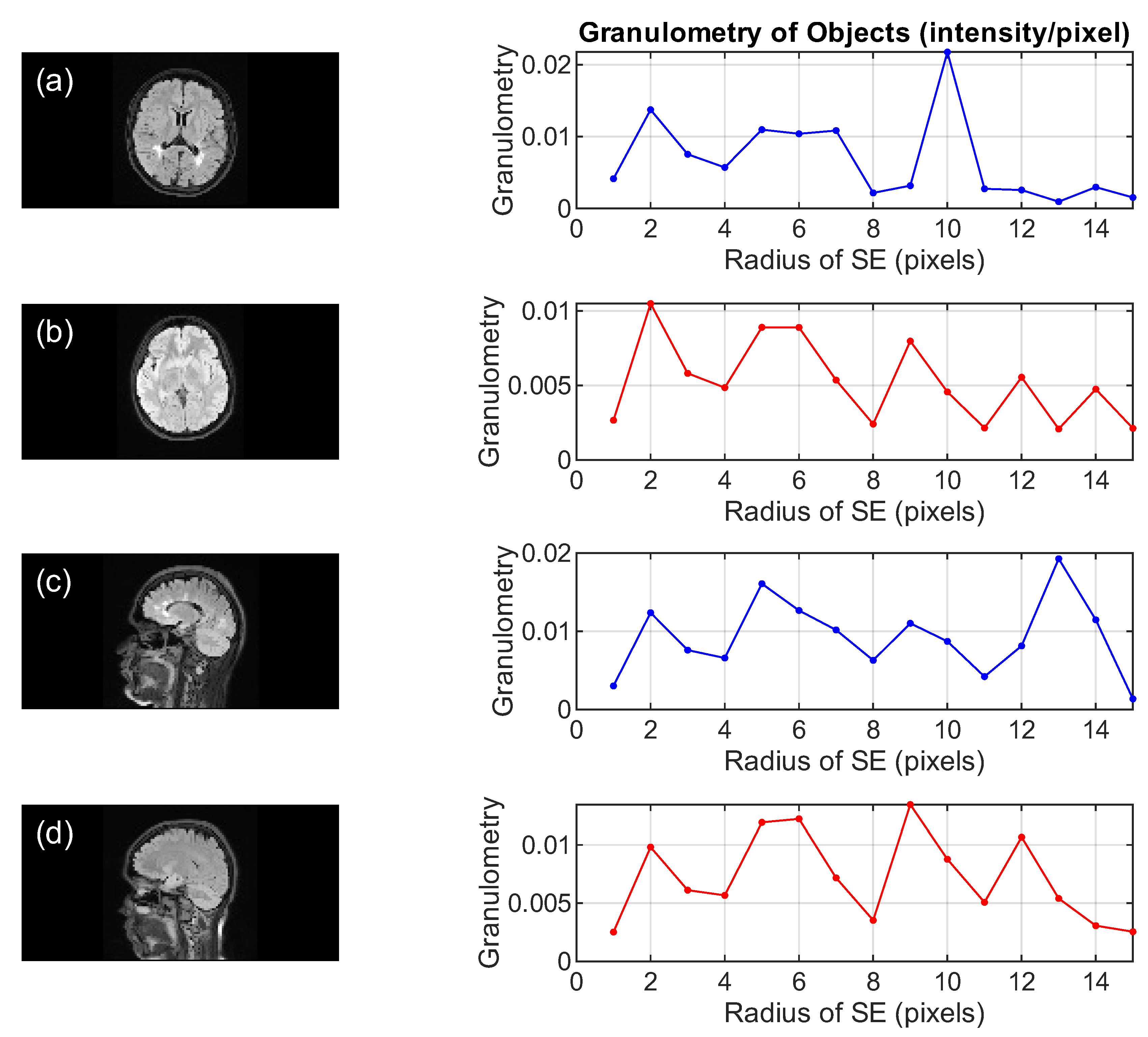
Figure 10.
Comparison of the sum of granulometry of objects. The sum of granulometry values in MS samples (axial and sagittal) is higher than in healthy ones.
Figure 10.
Comparison of the sum of granulometry of objects. The sum of granulometry values in MS samples (axial and sagittal) is higher than in healthy ones.
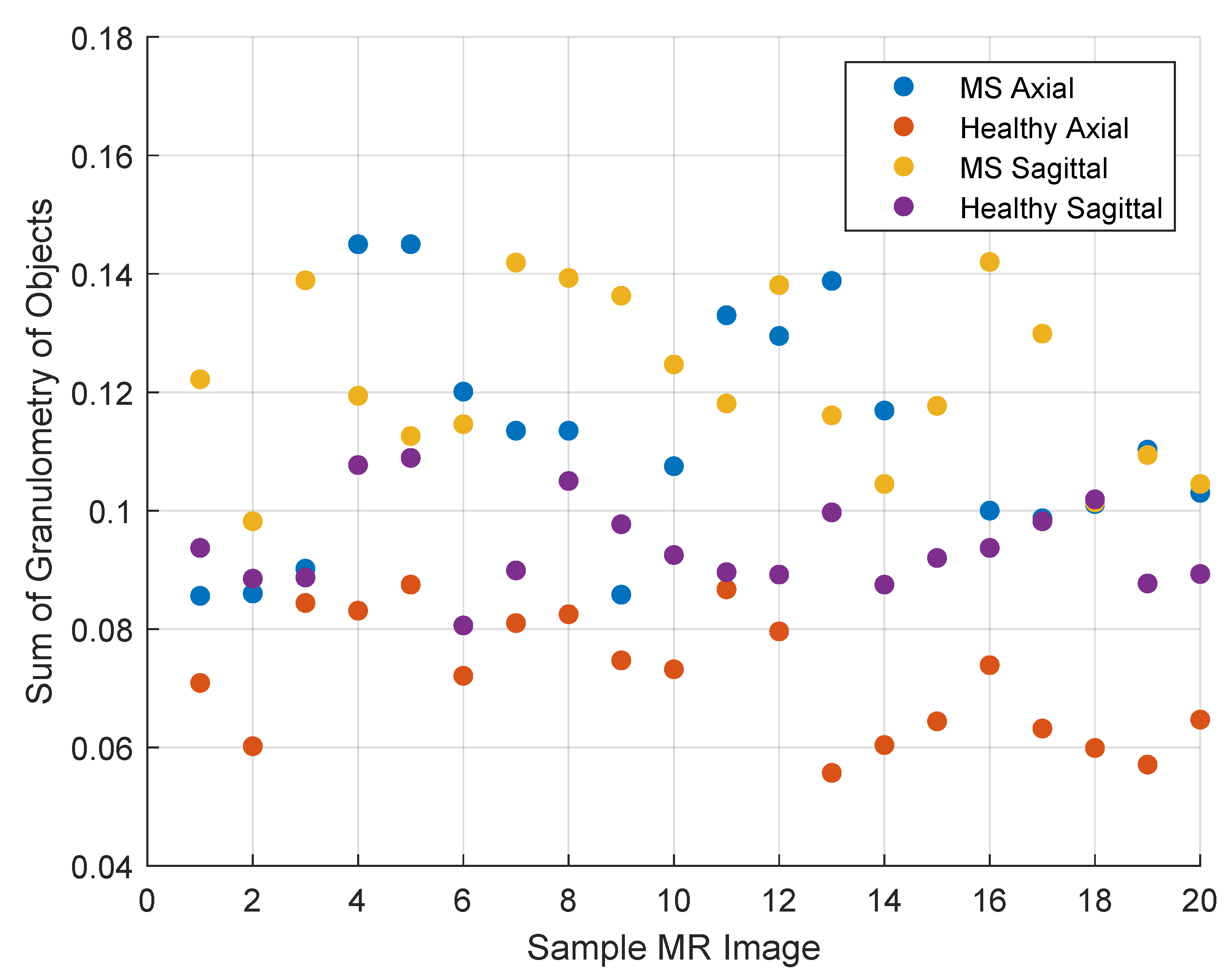
Figure 11.
Confusion matrix of predictions. TP = 10, TN = 10, FP = 0, FN = 0, for axial MRI. TP = 10, TN = 9, FP = 0, FN = 1, for the sagittal MRI.
Figure 11.
Confusion matrix of predictions. TP = 10, TN = 10, FP = 0, FN = 0, for axial MRI. TP = 10, TN = 9, FP = 0, FN = 1, for the sagittal MRI.

Figure 12.
Cross-entropy loss function vs regularization strengths graph. Lambda(axial)=0.005 and lambda(sagittal)=0.02 hyperparameters achieved the lowest loss values.
Figure 12.
Cross-entropy loss function vs regularization strengths graph. Lambda(axial)=0.005 and lambda(sagittal)=0.02 hyperparameters achieved the lowest loss values.
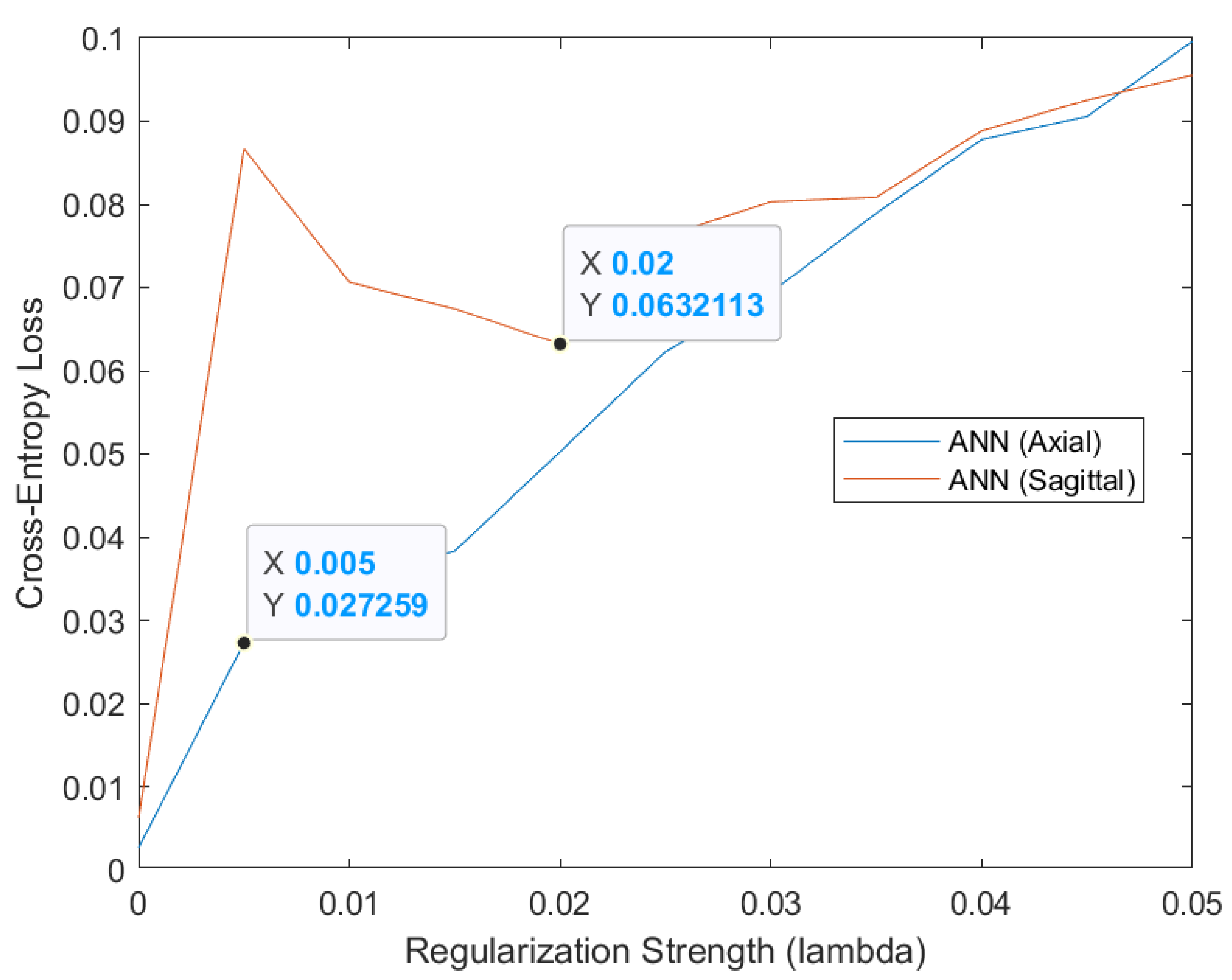
Figure 13.
Cross-entropy loss function behavior. The loss function of ANN (axial) converges faster than in ANN (sagittal).
Figure 13.
Cross-entropy loss function behavior. The loss function of ANN (axial) converges faster than in ANN (sagittal).

Figure 14.
Implementation of closing morphological transformations (MS axial). (a) Mask image (MS axial). (b) Mask image minus MS lesions. (c) Morphological closing. (d) Closing by reconstruction (reference image or healthy brain approach).
Figure 14.
Implementation of closing morphological transformations (MS axial). (a) Mask image (MS axial). (b) Mask image minus MS lesions. (c) Morphological closing. (d) Closing by reconstruction (reference image or healthy brain approach).
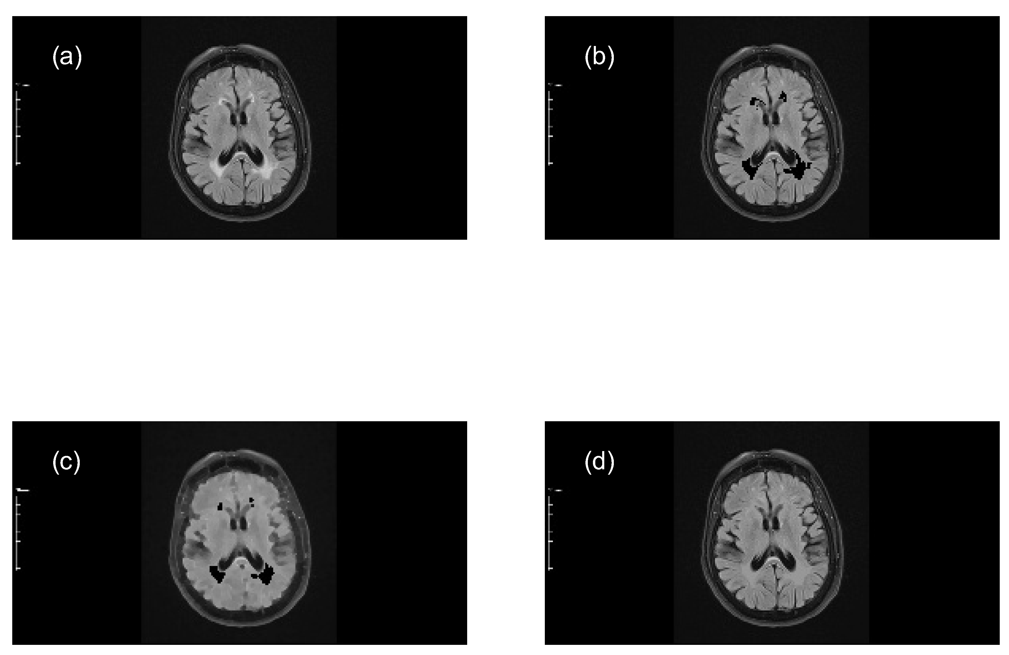
Figure 15.
Implementation of closing morphological transformations (MS sagittal). (a) Mask image (MS sagittal). (b) Mask image minus MS lesions. (c) Morphological closing. (d) Closing by reconstruction (reference image or healthy brain approach).
Figure 15.
Implementation of closing morphological transformations (MS sagittal). (a) Mask image (MS sagittal). (b) Mask image minus MS lesions. (c) Morphological closing. (d) Closing by reconstruction (reference image or healthy brain approach).
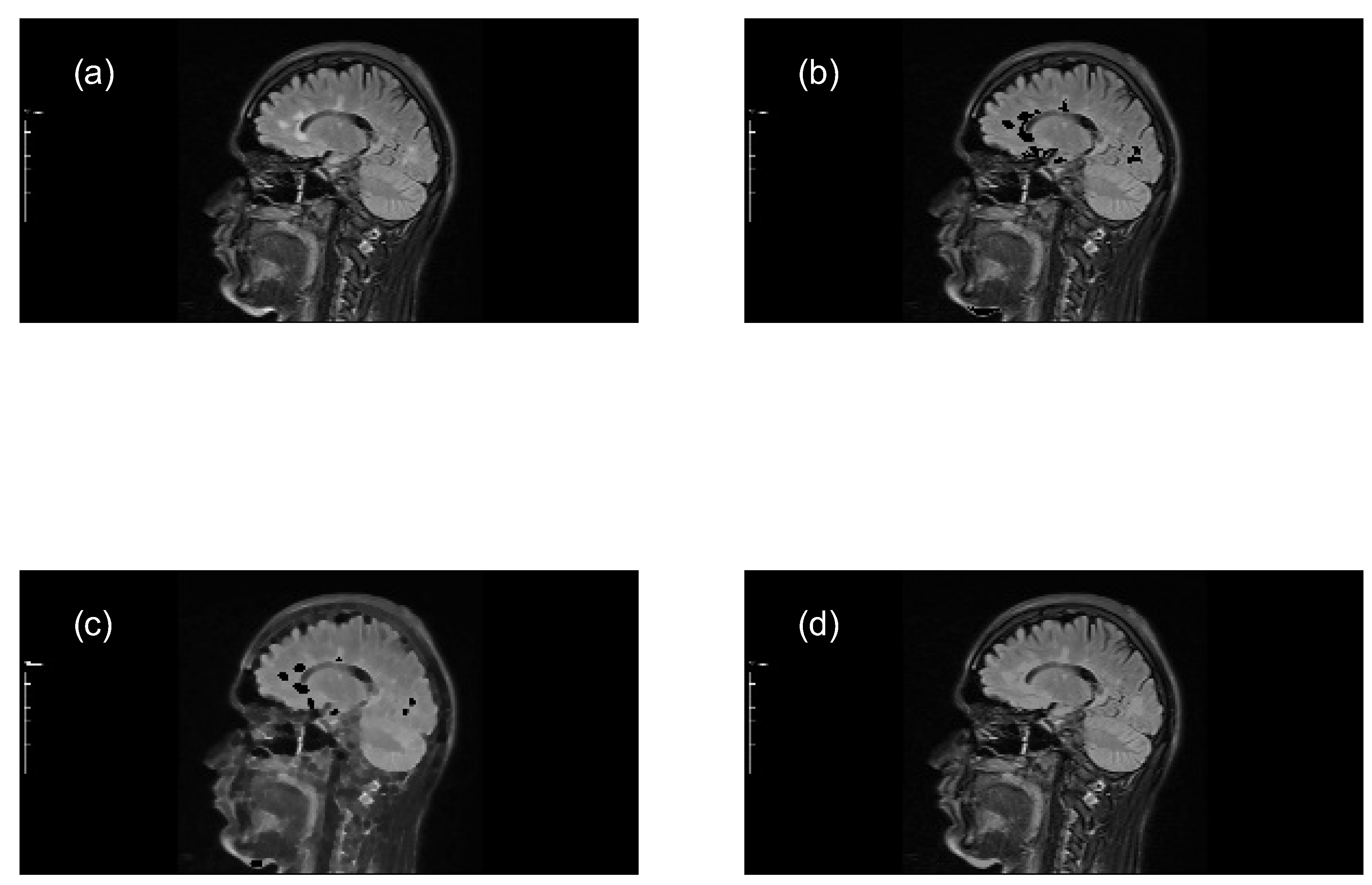
Figure 16.
Granulometry measurements (axial) of the mask image (with lesions) and the reference image (without lesions). The size of MS lesions is estimated by calculating the difference between each data point.
Figure 16.
Granulometry measurements (axial) of the mask image (with lesions) and the reference image (without lesions). The size of MS lesions is estimated by calculating the difference between each data point.
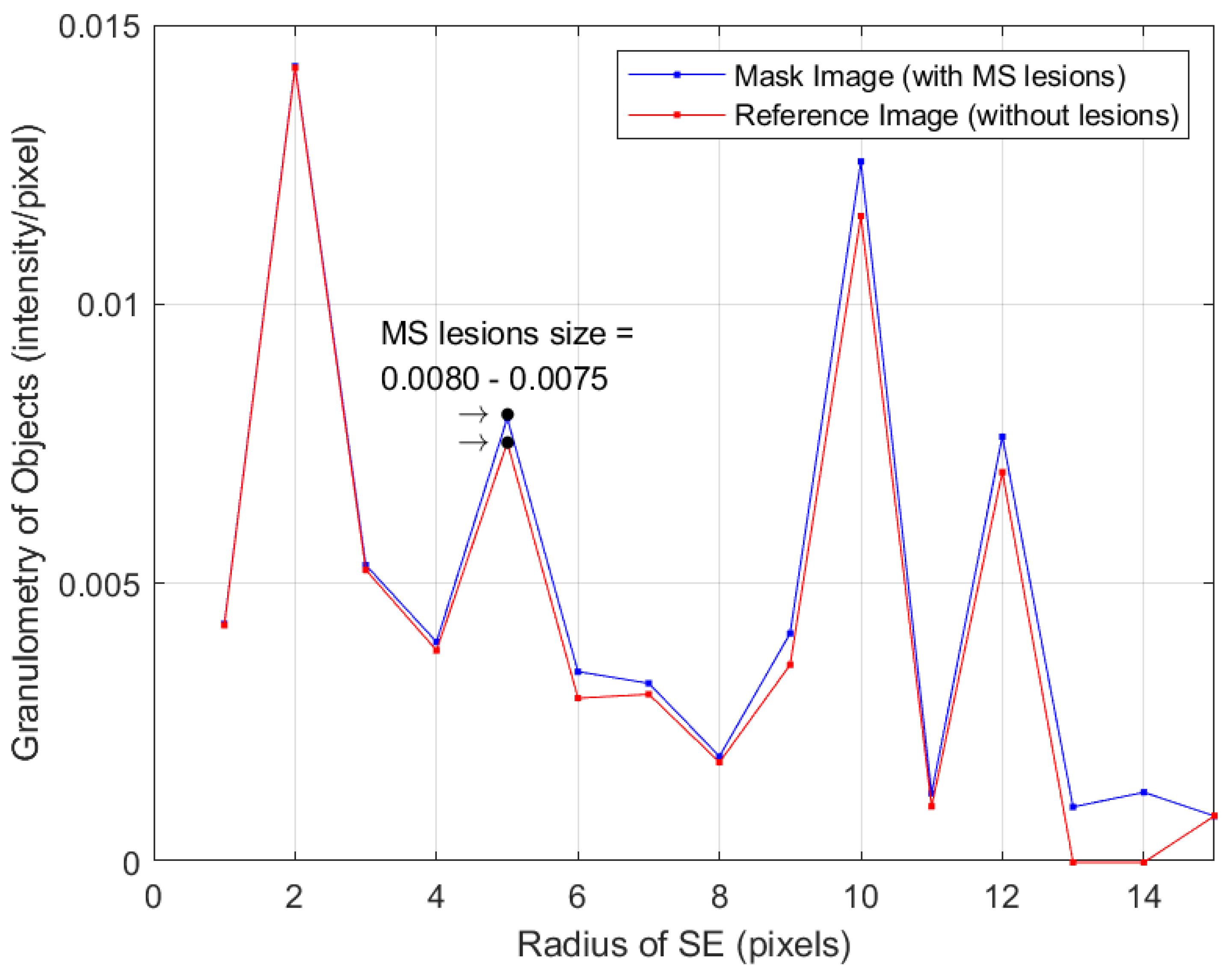
Figure 17.
Granulometry measurements (sagittal) of the mask image (with lesions) and the reference image (without lesions). The size of MS lesions is estimated by calculating the difference between each data point.
Figure 17.
Granulometry measurements (sagittal) of the mask image (with lesions) and the reference image (without lesions). The size of MS lesions is estimated by calculating the difference between each data point.
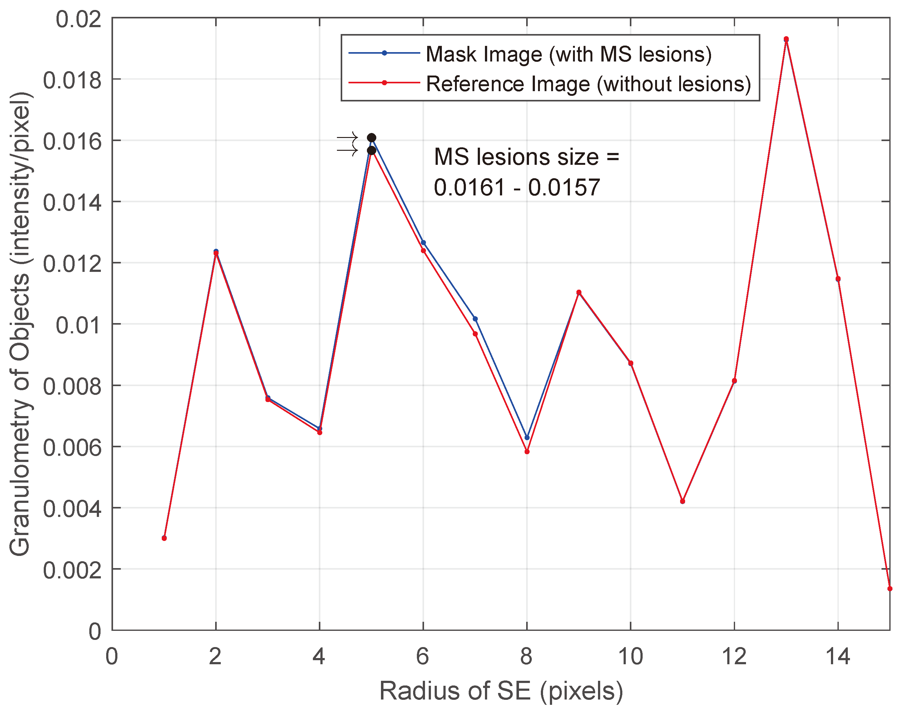

Table 1.
Implemented pseudocode of the MRI preprocessing algorithm (Stage 1).
| Pseudocode | ||
|---|---|---|
| Start | ||
| rgb = readImg(’sample’.png) | ||
| grayScale = rgbTogray(rgb) | ||
| maskImg = grayScale | ||
| markerImg1 = morphOpen(maskImg, SE 1(’disk’,5)) | ||
| openRec1 = openRec(markerImg1,maskImg) | ||
| MSlesions = intensityAdjust(openRec1) | ||
| volMaskImg1 = 1.0*sum(maskImg) | ||
| For | radius = 1:15 | |
| markerImg2 = morphOpen(maskImg, SE(’disk’, radius - 1)) | ||
| openRec2 = openRec(markerImg2, maskImg) | ||
| volOpenRec1 = sum(openRec2) | ||
| markerImg3 = morphOpen(maskImg, SE(’disk’, radius)) | ||
| openRec3 = openRec(markerImg3, maskImg) | ||
| volOpenRec2 = sum(openRec3) | ||
| volGranu(radius) = (volOpenRec1-volOpenRec2)/volMaskImg1 | ||
| End |
Structuring Element.
Table 2.
Implemented pseudocode of the MRI preprocessing algorithm (Stage 2).
| Pseudocode | ||
|---|---|---|
| Start | ||
| subtract = imgSub(maskImg, MSLesions) | ||
| markerImg4 = morphClose(subtract, SE(’disk’,radius=5)) | ||
| closeRec1 1 = closeRec(markerImg4,maskImg) | ||
| volMaskImg2 = 1.0*sum(closeRec1) | ||
| For | radius = 1:15 | |
| markerImg5 = morphOpen(closeRec1, SE(’disk’, radius - 1)) | ||
| openRec5 = openRec(markerImg5, closeRec1) | ||
| volOpenRec3 = sum(openRec5) | ||
| markerImg6 = morfOpen(closeRec1, SE(’disk’, radius)) | ||
| openRec6 = openRec(markerImg6, closeRec1) | ||
| volOpenRec4 = sum(openRec6) | ||
| volGranu(radius) = (volOpenRec3-volOpenRec4)/volMaskImg2 | ||
| End |
1 Reference image (without MS lesions).
Table 3.
Configured ANNs hyperparameters. Activations: Activation function for the fully connected layers in the ANN. Standardize: Flag to standardize the predictor data. Lambda: Regularization term strength, the software composes the objective function for minimization from the cross-entropy loss function and the ridge (L2) penalty term. LayerSizes: The ith element is the number of outputs in the ith fully connected layer of the ANN.
| Model | Activations | Standardize | Lambda | LayerSizes |
|---|---|---|---|---|
| (default) | (enabled) | (adjusted) | (default) | |
| ANN (axial) | ’relu’ | true | 0.005 | 10 |
| ANN (sagittal) | ’relu’ | true | 0.02 | 10 |
Table 4.
Computed granulometry values for 100 samples (axial).
| Sample | r=1 | r=2 | r=3 | ... | r=15 | Diagnostic |
|---|---|---|---|---|---|---|
| 1 | 0.0044 | 0.014 | 0.006 | ... | 0 | MS_Axial |
| 2 | 0.0038 | 0.0135 | 0.0087 | ... | 0.0176 | MS_Axial |
| ⋮ | ⋮ | ⋮ | ||||
| 50 | 0.0029 | 0.0108 | 0.0063 | ... | 0.0082 | MS_Axial |
| 51 | 0.0021 | 0.0075 | 0.0045 | ... | 0.0016 | Healthy_Axial |
| ⋮ | ⋮ | ⋮ | ||||
| 99 | 0.0023 | 0.009 | 0.0061 | ... | 0.0023 | Healthy_Axial |
| 100 | 0.0022 | 0.0089 | 0.0058 | ... | 0.0006 | Healthy_Axial |
Table 5.
Computed granulometry values for 100 samples (sagittal).
| Sample | r=1 | r=2 | r=3 | ... | r=15 | Diagnostic |
|---|---|---|---|---|---|---|
| 1 | 0.0025 | 0.099 | 0.006 | ... | 0.0017 | MS_Sagittal |
| 2 | 0.0018 | 0.0073 | 0.0044 | ... | 0.0024 | MS_Sagittal |
| ⋮ | ⋮ | ⋮ | ||||
| 50 | 0.003 | 0.0124 | 0.0074 | ... | 0.0037 | MS_Sagittal |
| 51 | 0.0022 | 0.009 | 0.0052 | ... | 0.0014 | Healthy_Sagittal |
| ⋮ | ⋮ | ⋮ | ||||
| 99 | 0.0019 | 0.0076 | 0.0042 | ... | 0.0019 | Healthy_Sagittal |
| 100 | 0.002 | 0.0082 | 0.0049 | ... | 0.0017 | Healthy_Sagittal |
Table 6.
Test accuracy and cross-entropy loss results.
| Model | Test Accuracy | DSC 1 | TPR 2 | TNR 3 | Cross-Entropy Loss |
|---|---|---|---|---|---|
| ANN (axial) | 0.9753 | 1.0 | 1.0 | 1.0 | 0.0247 |
| ANN (sagittal) | 0.9345 | 0.9523 | 0.909 | 1.0 | 0.0655 |
1 Dice similarity coefficient. 2 True positive rate. 3 True negative rate.
Table 7.
Performance results comparison of some studies in analyzing MS lesions.
| Image | |||
|---|---|---|---|
| Autor | Processing | Classifier | Performance |
| Technique | |||
| [16] | CEN | U-Net, U-Net++ | 0.7159 1 |
| Linknet | |||
| [19] | ExMPLPQ | kNN | 0.9837 3 |
| 0.9775 4 | |||
| [20] | Lesion volume | CNN | 0.9786 1 |
| quantification | 0.9969 2 | ||
| [21] | CNN | CNN | 0.98 5 |
| 0.903 6 | |||
| [22] | Attention | Modified | 0.823 1 |
| U-Net | U-Net | ||
| [23] | U-Net | U-Net++ | 0.88 1 |
| [24] | Augmented U-Net | LSTM | 0.89 1 |
| Our paper | Morphology & | ANN | 1.0 1 |
| Granulometry | 0.9654 3 | ||
| 0.9437 4 |
1 Dice similarity coefficient. 2 Accuracy. 3 Accuracy (axial). 4 Accuracy (sagittal). 5 Accuracy Cutting-level. 6 Accuracy Patient-level.
Disclaimer/Publisher’s Note: The statements, opinions and data contained in all publications are solely those of the individual author(s) and contributor(s) and not of MDPI and/or the editor(s). MDPI and/or the editor(s) disclaim responsibility for any injury to people or property resulting from any ideas, methods, instructions or products referred to in the content. |
© 2024 by the authors. Licensee MDPI, Basel, Switzerland. This article is an open access article distributed under the terms and conditions of the Creative Commons Attribution (CC BY) license (http://creativecommons.org/licenses/by/4.0/).
Copyright: This open access article is published under a Creative Commons CC BY 4.0 license, which permit the free download, distribution, and reuse, provided that the author and preprint are cited in any reuse.


