Submitted:
20 July 2024
Posted:
23 July 2024
You are already at the latest version
Abstract
Which machine-learning model is the best at winning the prisoner’s dilemma? Which models create the best cumulative outcomes? Is there a model that perfectly captures both winning and cumulative points? These are questions generated from a simple 2 x 2 payoff matrix of the prisoner’s dilemma. Imagine you and your partner in crime are caught and sent independently into questioning. You can either collaborate or defect, but you don’t know what your partner will do. If you both collaborate, cumulatively, you’ll each get one year in jail. If you defect and your partner collaborates, you’ll serve no time and they will serve 10 years, and vice versa. If you both defect, you’ll both serve 5 years in jail. Placing AIs against each other to play just one round doesn’t reveal much about their code, strategy, and end goal. So the Reinforcement Learning, Pattern Learning, Tit For Tat, and other models were put up against each other in a 100 round game where their behavior, convergence, and learning were analyzed to reveal the most effective ways strategies to beat the prisoner’s dilemma. All code and data is open sourced here.
Keywords:
Game Theory
; Prisoner's Dilemma
; Machine Learning
1. Introduction
Research surrounding the implications of machine-learning on the Prisoner’s Dilemma has been primarily focused on Reinforcement Learning and the Tit-for-Tat strategy. The intention of this project is to analyze head-to-head match-ups between various machine-learning and game-theoretic algorithms and provide a statistical lens to view the 70-year-old dilemma.
The simulation in this project is a 100-round iterated Prisoner’s Dilemma game. The game was programmed in Java and takes two Players and simulates the game based on each player’s pre-programmed strategy while their learning models actively gain memory and experience that inform their moves. Some strategies are simple like AlwaysDefect and some are more complicated like the PatternLearner. Each player will gain points based on the reward matrix below.

Table 1.
Reward Matrix
| C | D | |
|---|---|---|
| C | +3 +3 | +5 +0 |
| D | +0 +5 | +1 +1 |
2. Meet The Players
The first player is the QLearningPlayer, a Reinforcement Learning model that makes decisions based on real-time Q-value updates. This model is fitting because Q-Learning allows the player to balance exploration (moving randomly) and exploitation (comparing Q-values) and eventually converge to an optimal policy (C or D) based on the reward given per round. Q-values are updated and calculated using the Bellman equation:
where is the learning rate, is the discount factor, r is the reward, is the next state, and b is the next action. In the implementation of the game, the player class records the current state with each reward and updates its Q-values based on each move. is set to 0.1, to 0.9, and exploration rate is set to 0.6 with a decay rate of 0.99 per round. These values are arbitrarily set but enable the model to learn and decrease exploration as the model is trained. Each Q-value for each move C or D is tracked in a HashMap with a double array and the player will collaborate or defect depending on which Q-value is higher.
In the first model, the reward system is set to account only for the player’s personal reward (which would be values of 1, 3, or 5). This could lead to the player commonly converging to defection to maximize its own reward of 5. To explore the differences between personal reward and cumulative reward, a model called the JointPQLearningPlayer was created. This player considers the state of all players’ moves (e.g., CC if both players collaborated) as opposed to the traditional account of one move (C if opponent collaborated). Additionally, this model’s reward updated in the Bellman equation is the cumulative reward which would be values of 5, 6, or 2 for states CD or DC, CC, and DD respectively.
The next strategy is the BayesianInferencePlayer (BIP). This model is programmed to calculate the probabilities of each of the opponents’ moves to structure the BIP’s next move.
The model uses the equations above, where and represent the BIP’s probability of C and D respectively, with and representing the number of times the opponent has C and D and t representing the total amount of moves. For example, if the model predicts that there is an 80% chance that the opponent will C, there will also be an 80% chance that the BIP will also C. The values of and are initialized to 1 and t to 2 for Laplace Smoothing to avoid the case of dividing by zero.
But what if we took the base idea from the BIP and took it a step further? The next strategy is the PatternLearningPlayer (PLP) which makes predictions based on the history of the opponent’s moves. This player uses a simple n-gram model for sequence prediction and is visually depicted in Figure 1.
With a set history of 3, the PLP moves randomly for 3 rounds to collect data on the opponent’s strategy. Each pattern is stored in a HashMap and then the model can predict, for example, if the opponent will C or D given a history of CCD based on the amount of the times the opponent’s next move has been C or D given that state. The player will play whichever move is predicted of the opponent.
The next strategy is a game-theoretic strategy called TitForTat. This player’s strategy revolves around doing the same move that the opponent had previously done. This strategy is especially interesting because it can “train” other models by giving them a taste of their own medicine. This gives them a punishment if they previously defected and a reward if they previously cooperated. Additionally, a reverse Tit-for-tat (revTitForTat) player was created who plays the opposite move that the opponent previously played.
The next player is the Upper Confidence Bound (UCB) Player which creates a bound for each move C or D and moves based on the larger UCB bound. This is a reinforcement learning algorithm that balances exploration and exploitation with the following equation:
where is the mean reward for action a, t is the total number of times all actions have been played, and is the number of times action a has been played. represents exploitation and the confidence interval term represents exploration and ensures that fewer-played actions get the chance to the played. By increasing the confidence interval for less played, the UCB ensures each action is explored before converging to a sub-optimal C or D.
Another game-theoretic player was added to test the limits and the cooperation levels of the different models. The Grudge Player begins with collaboration but once the opponent defects, the Grudge Player defects twice before going back to collaboration.
The next player is the PatternPlayer. Rather than C or D using a mathematical expression, the player moves based on a predetermined pattern. The numerical pattern is 01121220 and if there is a zero, the player C and if there is a one, the player D. When a two is encountered, those roles swap. The pattern for one complete iteration is shown below.
Finally, a couple of other basic player models were created to diversify the player pool. A player that always collaborates, a player that always defects, a player that alternates between the two, and one that moves completely randomly were added.
3. Predictions
This results in five categorizations of the models. Firstly, the game-theoretic models that make decisions based on their opponents’ moves. Next, the learning models who prefer cumulative reward like how the PatternLearner’s and BayesianInference’s models collaborate if they predict an opponent collaboration. The JointPQLearner updates its Q-values based on combinations of points which allows it to move as such. Next, the machine learners who are rewarded based on their own points gained and make decisions based on those. Next, the unchanging patterns which is self-explanatory. Lastly, the random player who is just random.
Table 2.
Model Categorizations
| Game-Theoretic | Learners (cumulative reward) | Learners (individual reward) | Unchanging Patterns | Random |
| TitForTat | PatternLearner | QLearner | Alternates | Random |
| revTitForTat | JointPQLearner | UCBPlayer | PatternPlayer | |
| grudgePlayer | BayesianInference | AlwaysC | ||
| AlwaysD |
By the end of the data processing stage, we will want to know the average cumulative scores to see how collaborative each match-up is, the number of CCs to better understand how each point total was played, and the win rates to see how competitive each player is. An initial prediction from looking at the categories is that the Game-Theoretic strategies will have the highest win rates (as they are programmed to be reactive rather than based on points), cumulative reward learners will have the highest cumulative scores and CCs, and individual reward learners will have a lower cumulative score but higher win rate.
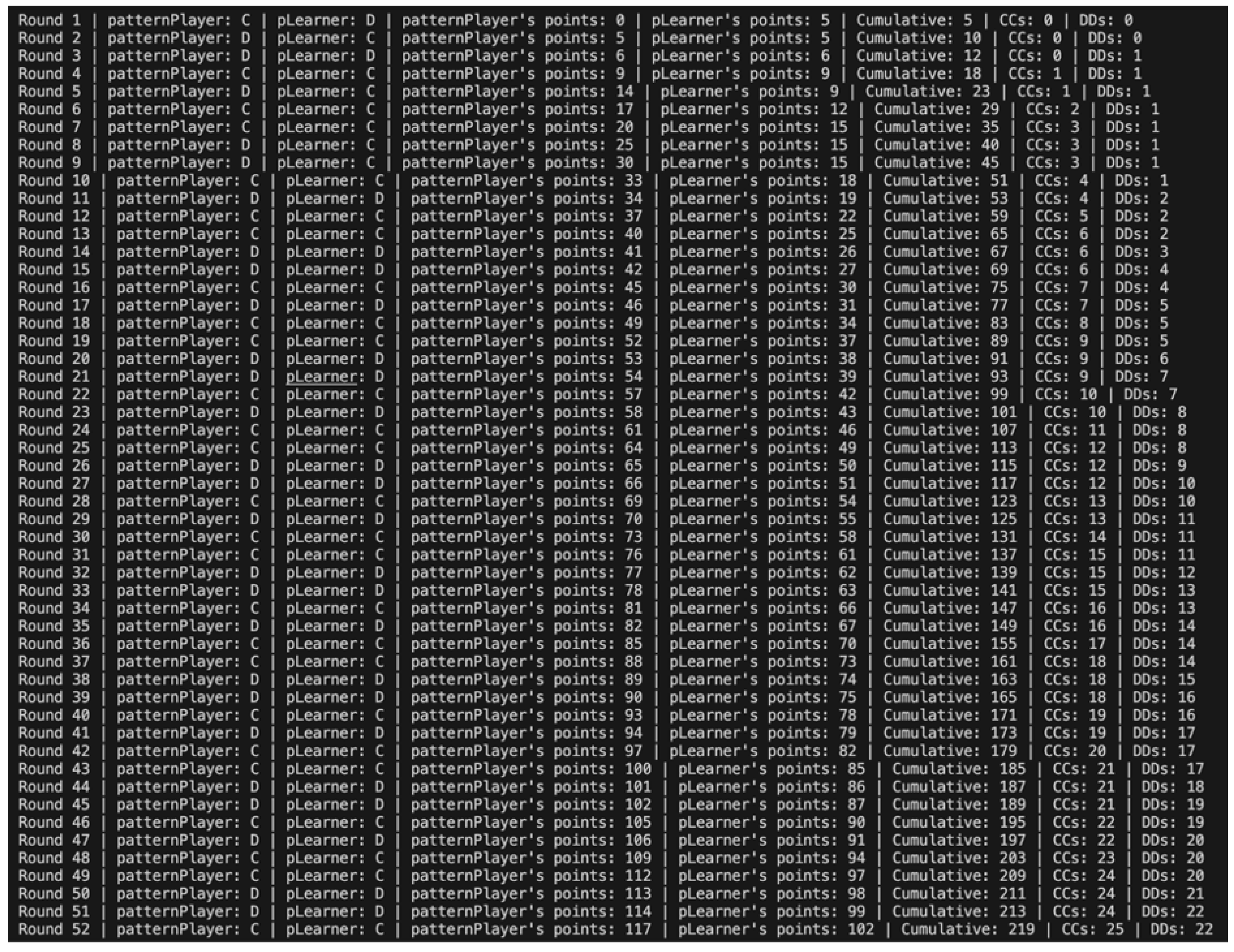
4. The Game
Displayed above is the terminal output of one 100-round game of the Pattern Player vs. the Pattern Learning Player. While not all 100 rounds are displayed, the program runs for a set number of iterations and tracks all point totals and times the players both collaborated and both defected to track cooperation levels. Each will play every player for a calculated number of games (not to be confused with rounds; each game has 100 rounds). The number of games will be calculated based on the sample size for a mean with a margin of error of 1 and a confidence interval of 95%. After each ten-round pilot study, the total amount of games is calculated for each player using:
where Z, the Z-value corresponding to the desired confidence level, is 1.96, E, the desired margin of error, is 1, and , the standard deviation, is estimated per match-up. The game model will take the standard deviation of the cumulative scores in the pilot study to estimate the standard deviation. After the pilot study, the model will dynamically resize the number of games needed for each player and will run those games into the generated database. The greatest number of rounds played between two players was 11,869,200 by the PatternLearningPlayer and the GrudgePlayer! The CSV dataset for each player will include the variables: Game, Opponent, PlayerA_Score, PlayerB_Score, Cumulative_Score, CCs, DDs, and Winner.
Figure 2.
Game Terminal Output
The terminal output for the simulation ran for the QLearningPlayer (where the QLearner is playerA) is shown in Figure 3 and the beginning of the 17529-row dataset is shown in Figure 4. Most of the names should be self-explanatory, but Gullible is Always Collaborate, Sly Fox is Always Defect, Randy is Random, and Evan is Alternate Collaboration. All data structures containing “memory” of the learning players were reset from game to game, ensuring that the models are only learning between rounds, not independent games – otherwise, data points would repetitively converge to one score.
This process created nine datasets with each playing player (all players except the four noted not to play each other) which were processed and merged to create a database with usable numbers.
5. Processing
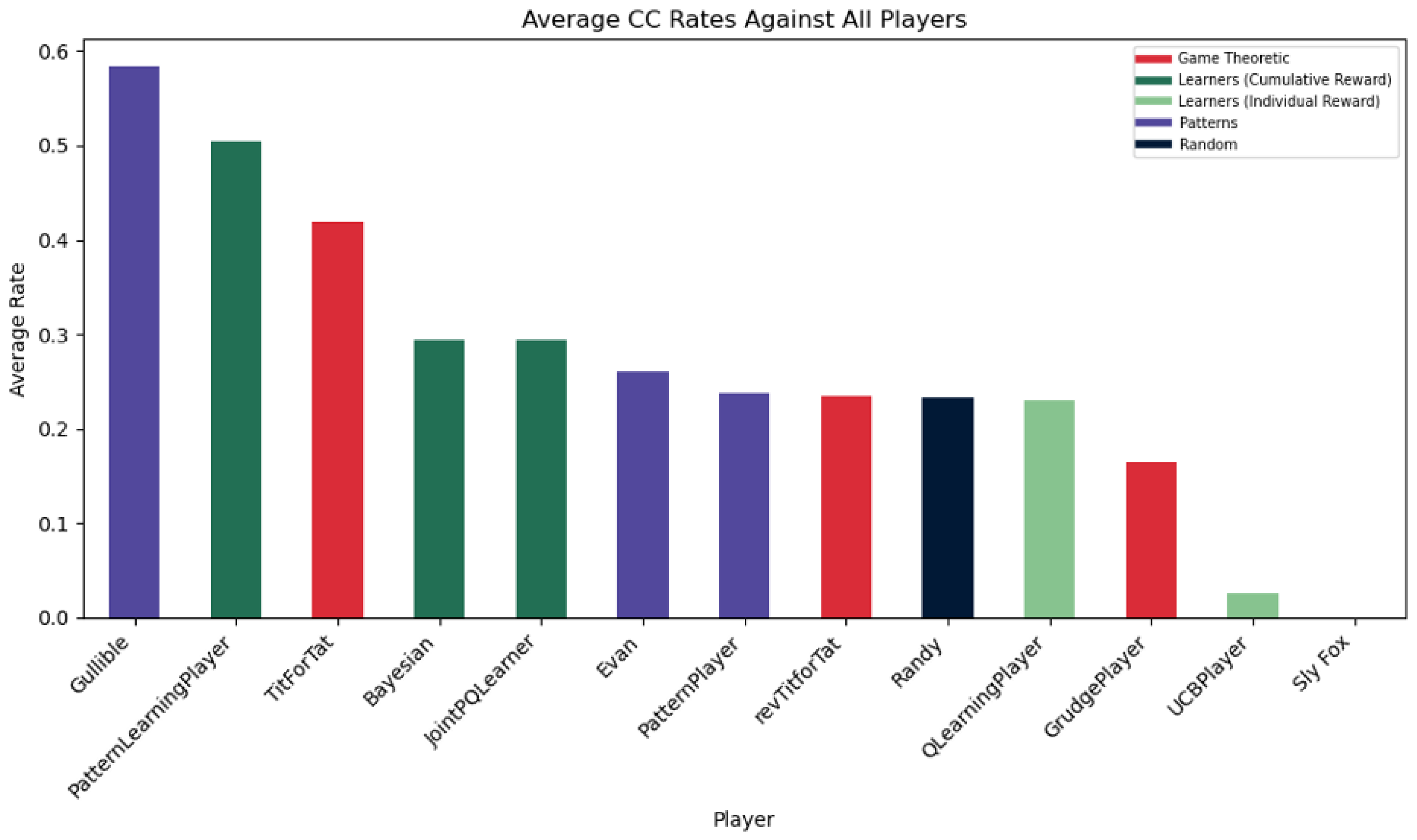
Once all nine datasets were created, they entered a procedural stage where they were processed and merged into 3 data frames which show the results of each match-up with our variables of interest: Cumulative Scores (Figure 5), Win Rates (Figure 6), and CC Rates (Figure 7).
Each of these data frames include all relevant analysis from the large datasets that included scores from each game.
6. Results
After the processing stage, the result of the AlwaysCollaborate (Gullible) player encouraging the highest average score total is not a surprise – it collaborates every time! Additionally, the prediction of the Cumulative Reward Learners performing well in point totals held up in Figure 8 – with the JointPQLearner creating the highest score out of any non-pattern player. This is logical because the model gains the most personal reward when both players collaborate and will get lower reward if there is any defection. The surprise is the PatternLearningPlayer’s algorithmic complexity under-performing compared to the Bayesian player’s straightforward calculations. This reveals that specificity doesn’t always result in more allocative results.
For the Game-Theoretic players, an interesting pattern will be noticed within the next coming figures. The revTitForTat consistently shows up between TitForTat and the GrudgePlayer seemingly acting as a median of the two. This contextually makes sense in this visualization because TitForTat encourages collaboration more than the reverse model and definitely more than the GrudgePlayer who often likes defection twice as much as its opponent. It is interesting to also conceptually think of revTitForTat as the middle ground between the two because they all handle defection and collaboration in similar ways.
Obviously, the AlwaysDefect (Sly Fox) remains on top in Win Rates – constant defection is the dominant strategy which means it literally cannot lose (it can tie which is why the win rate is not 100%). Figure 9 further supports the prediction of Individual Reward Learners performing well in win rates; players like the UpperConfidenceBound can identify that defection is key to higher point totals. However, the surprise is in successful Game Theoretic GrudgePlayer. The rate makes sense as it punishes its opponents for defection with double the loss (by defecting twice when receiving a defection) which may result in constant defection similar to the Sly Fox’s game model.
Despite the hype, the TitForTat player curiously under-performed in this category – proving that the player may not be the most offensive. Upon further inspection, it was because the TitForTat player has a tie rate of 77% which reveals the efficacy of the TitForTat player in accumulating a lot of points but not winning in a margin over the opponent. This also makes sense because the TitForTat player makes decisions reactive to the opponent and will copy the opponent’s pattern.
Again, the AlwaysCollaborate (Gullible) player being the most collaborative is not a surprise because it always collaborates. Expectedly, the PatternLearningPlayer (a popular choice now) takes the spot as the most effective at predicting and making CCs happen. Interestingly, TitForTat, a model that is able to train the opponent to collaborate, performs better than the JointPQLearner who is rewarded when both models collaborate. This reveals that punishing the opponent for defecting may be more effective than only one of the two players encouraging collaboration.
The behavior of the Evan (Alternate) PatternPlayer, revTitForTat, and Randy (random) statistically make sense, hovering around the 25% mark. Out of the four possible outcomes (CC, CD, DC, DD), it would be a 25% chance to CC given that the strategies are mostly random and pattern-based. This implicates how the QLearningPlayer moves as well, suggesting that its behavior behaves similarly to a simple ¼ probability. Upon further investigation, it was found that the DD rate was also 25%. It makes sense that the CC rate would match the DD rate since the QLearningPlayer balances both exploitation and exploration. However, I don’t believe that there is as much significance that the rates are both around 25% since the numerical values are based on the player pool and which strategies the model is competing against.
The player combinations that had the highest cumulative scores of 600 points (the max points they could attain) were the GrudgePlayer with TitForTat, TitForTat with TitForTat, and those players with AlwaysCollaborate. The best performing combination of learning models was the PatternLearner with the Bayesian player with approximately 596 points. The worst combinations were the GrudgePlayer with itself at a total of approximately 200 and the GrudgePlayer with the UCBPlayer with also 200 points.
To emphasize the game in game theory, the players were placed in a bracket to decide the most ruthless and individualistic prisoner’s dilemma winner. AlwaysDefect cannot lose and AlwaysCollaborate cannot win, so they were excluded from the bracket. The 11 players were seeded by their win rates and to stay true to the inherent nature of a competition, they were only allowed to play one round which will decide who moves on. Ties will result in the next non-tie game being recorded.
Figure 11.
Tournament Bracket
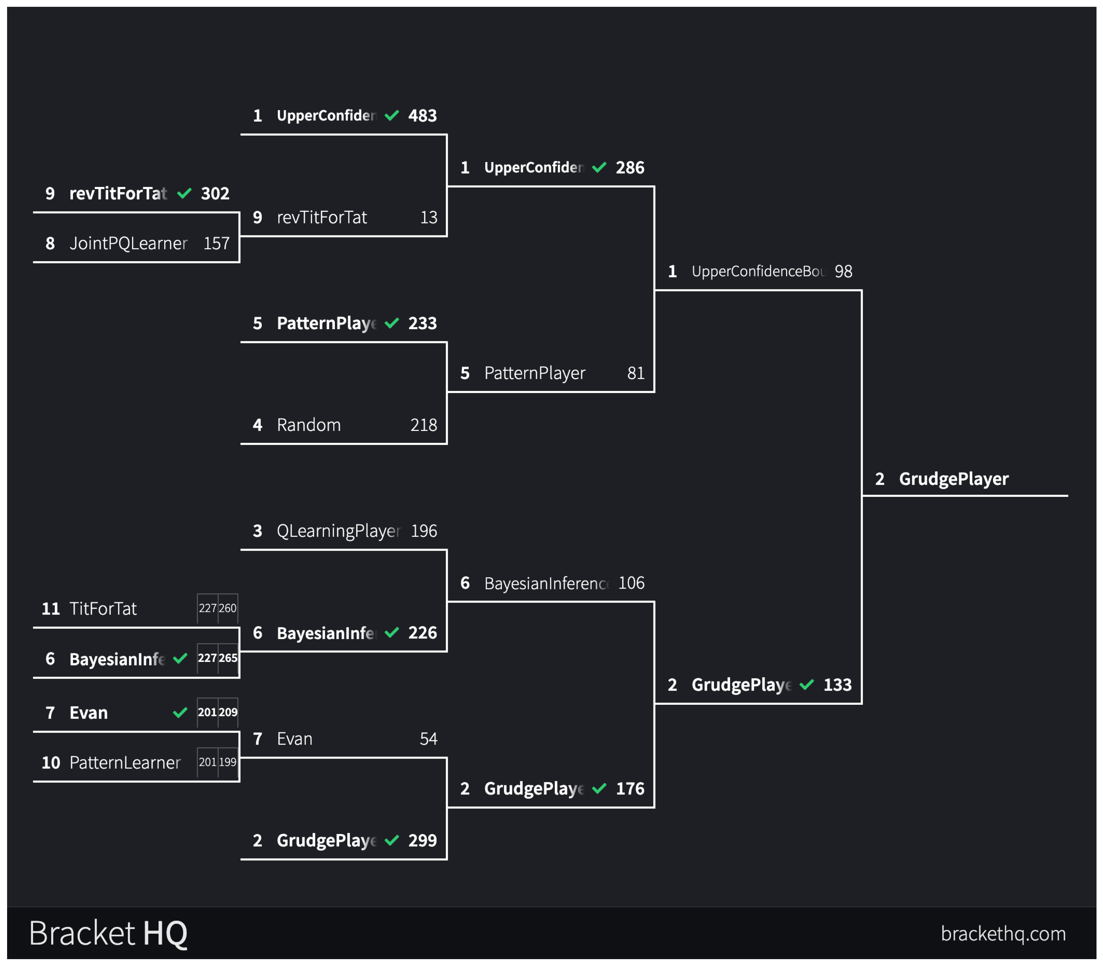
As the game progressed, it looked as if No. 1 UpperConfidenceBound was going to take the game after having a dominant win streak but ultimately it was the No.2 seed GrudgePlayer in a slight upset to run away with the victory in the lowest point game in the entire tournament. The fact that commonly defecting strategies did better in the bracket while decreasing total game points illustrates the payoff matrix’s trade-off in prioritizing wins. Interestingly, in the first round both No. 11 TitForTat vs. No. 6 BayesianInference and No. 10 PatternLearner vs. No. 7 Evan both initially tied but it wasn’t enough to pull the upset.
7. Conclusion
As the winner of the bracket reveals, in a simple game like the Prisoner’s Dilemma where a player can only either collaborate or defect, sometimes a simple strategy with just 27 lines of code beats a complicated mathematical algorithm. Starting all the way back at the matrix, there are only two results the players can have: the allocative result or the selfish result. The simulation holds true that players whose programs are embedded with allocative rewards move for cumulative good while individual reward systems move selfishly.
If a player’s only goal is to win the round, it should defect every time as it is the dominant strategy from the payoff matrix. The nuance comes when players want to maximize cumulative good – learning to trust and predict moves is key. This necessitates a model who is encoded with cumulative good within its decision-making process (the cumulative reward learners) or the ability to train other models away from defection (like the TitForTat model).
This may come as an intuitive thought but in the context of broader decisions involving outcomes more than just CC, CD, DC, and DD, this simulation informs us that decisions will be made according to a player’s essential nature. So when picking your partner-in-crime make sure that they are not either a Sly Fox, a grudge holder, or someone who operates based on the Upper Confidence Bound.
References
- Sandholm, Tuomas W, and Robert H Crites. “Multiagent Reinforcement Learning in the Iterated Prisoner’s Dilemma.” Science Direct, Elsevier Ireland Ltd., 26 Apr. 1999, http://www.sciencedirect.com/science/article/abs/pii/0303264795015515.
- “Upper Confidence Bound Algorithm in Reinforcement Learning.” GeeksforGeeks, GeeksforGeeks, 19 Feb. 2020, http://www.geeksforgeeks.org/upper-confidence-bound-algorithm-in-reinforcement-learning/.
- Veritasium. “What Game Theory Reveals about Life, the Universe, and Everything.” YouTube, YouTube, 23 Dec. 2023, http://www.youtube.com/watch?v=mScpHTIi-kM.
- Surma, Greg. “Prison Escape - Solving Prisoner’s Dilemma with Machine Learning.” Medium, Medium, 11 Apr. 2019, http://gsurma.medium.com/ prison-escape-solving-prisoners-dilemma-with-machine-learning-c194600b 0b71.
Figure 1.
PatternLearning Algorithm
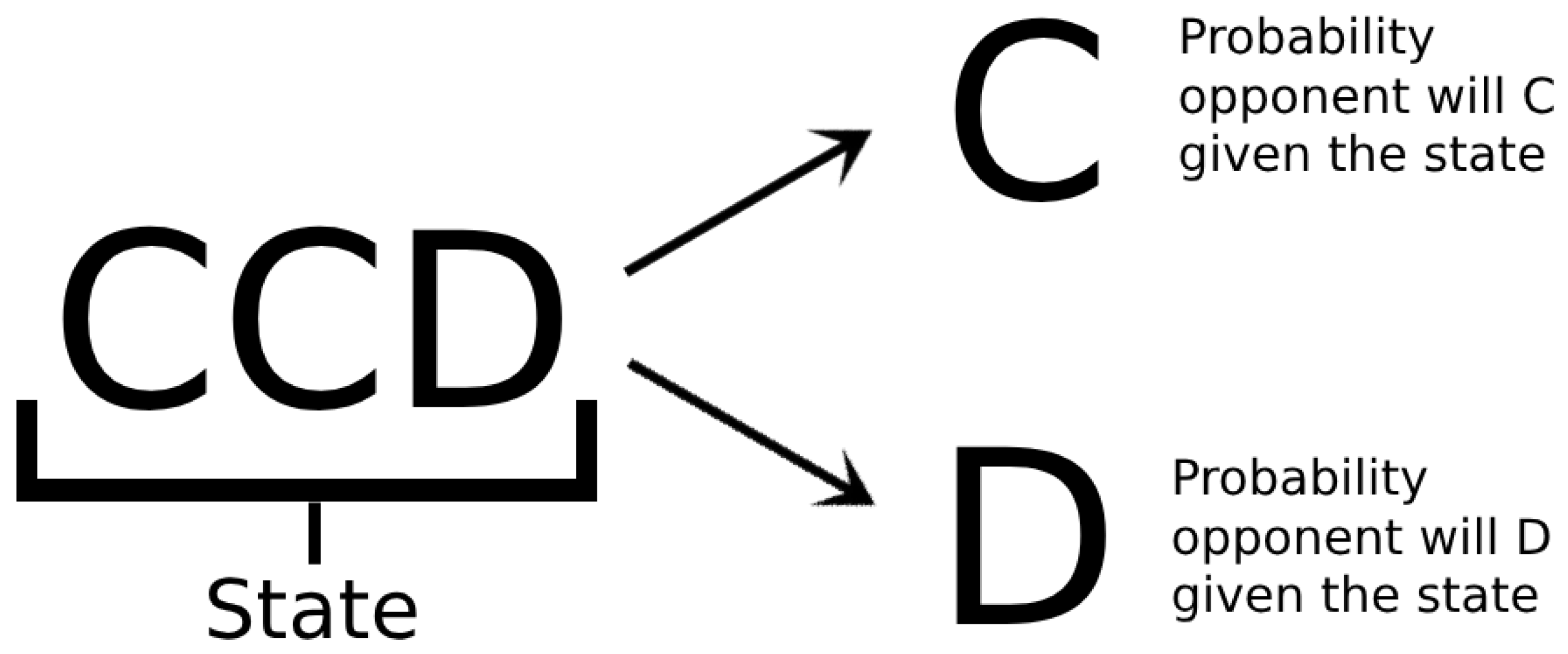
Figure 3.
Simulation Terminal Output
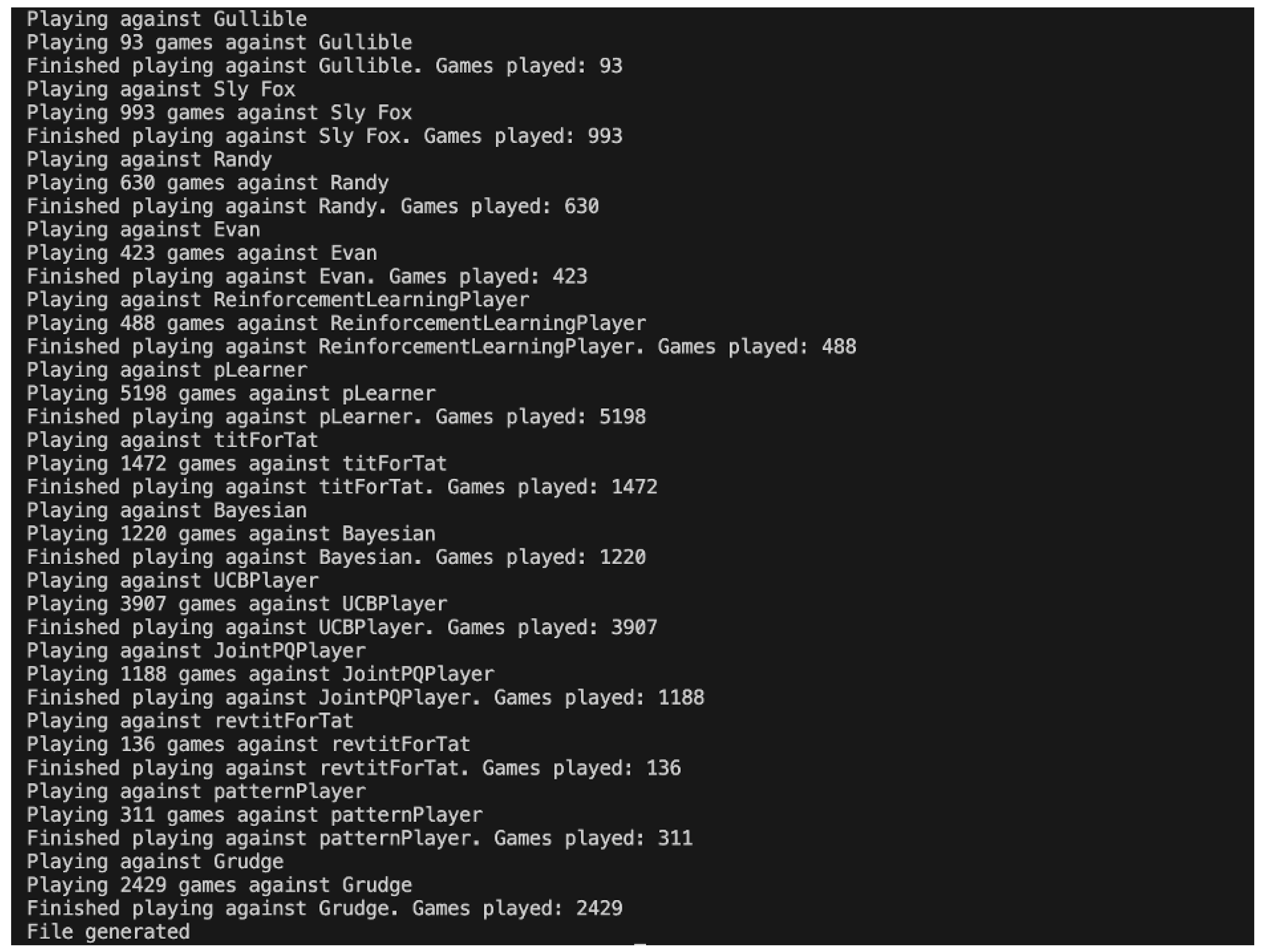
Figure 4.
QLearner Dataset
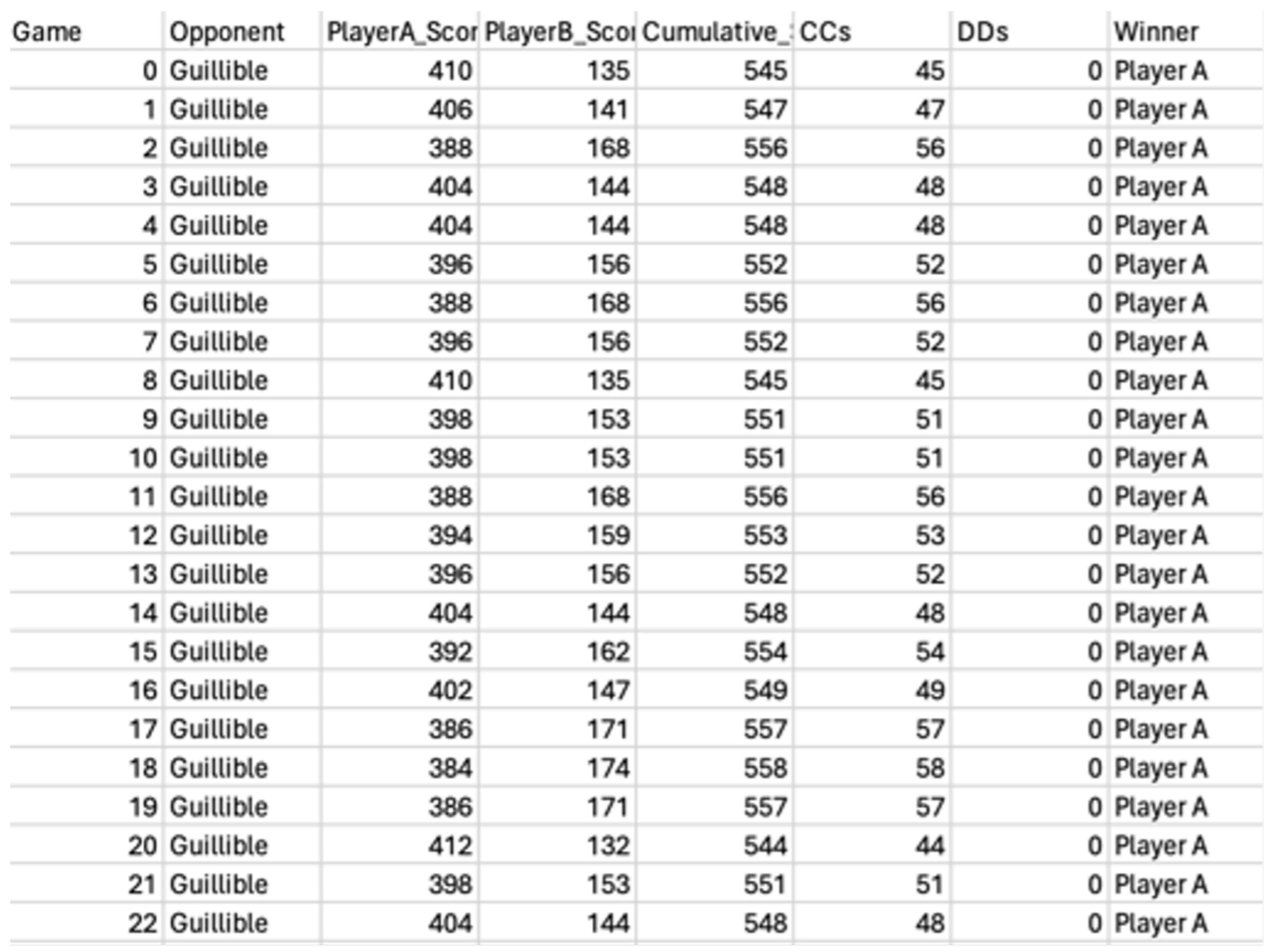
Figure 5.
Cumulative Scores
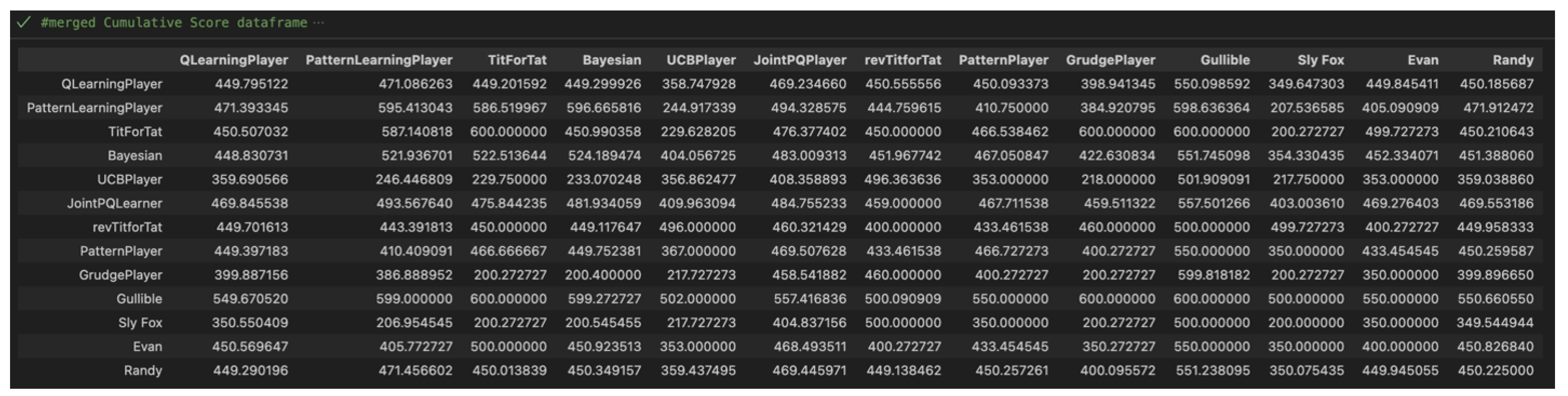
Figure 6.
Win Rates
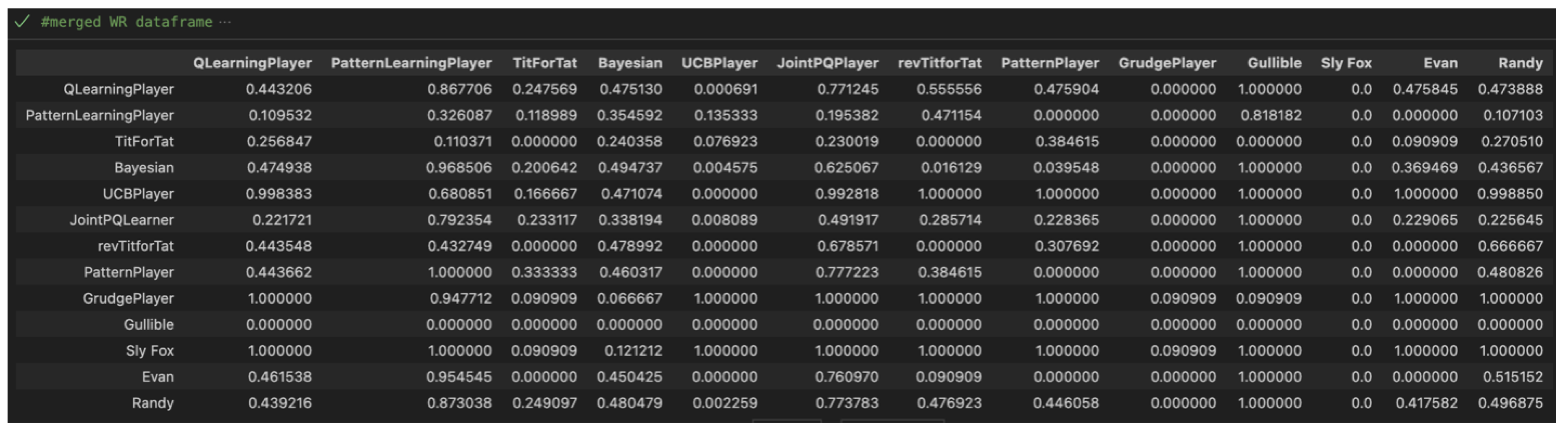
Figure 7.
CC Rates
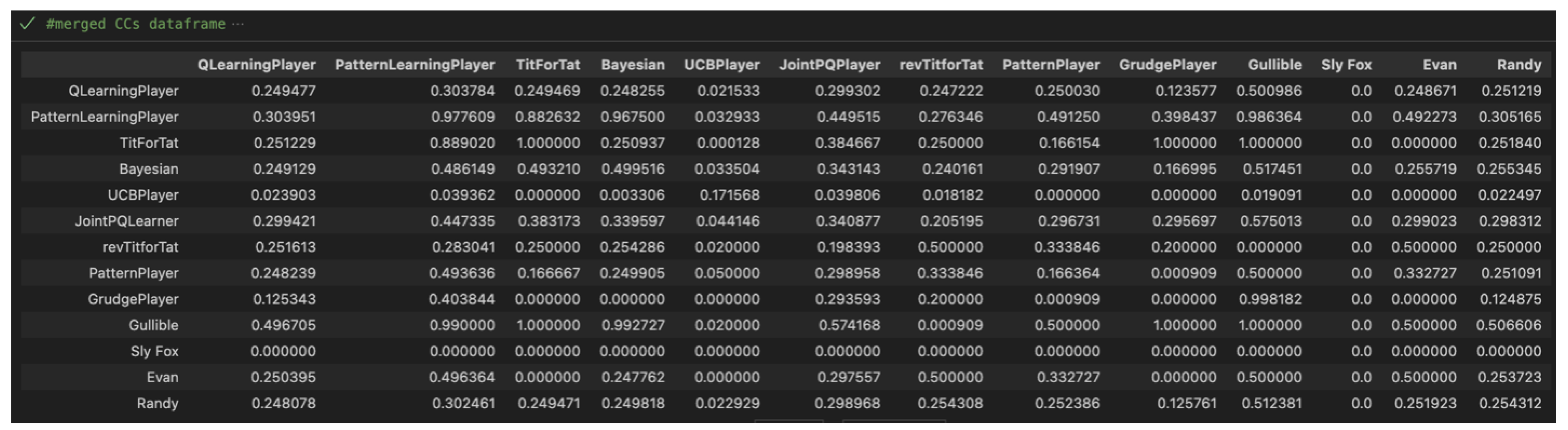
Figure 8.
Results Overview
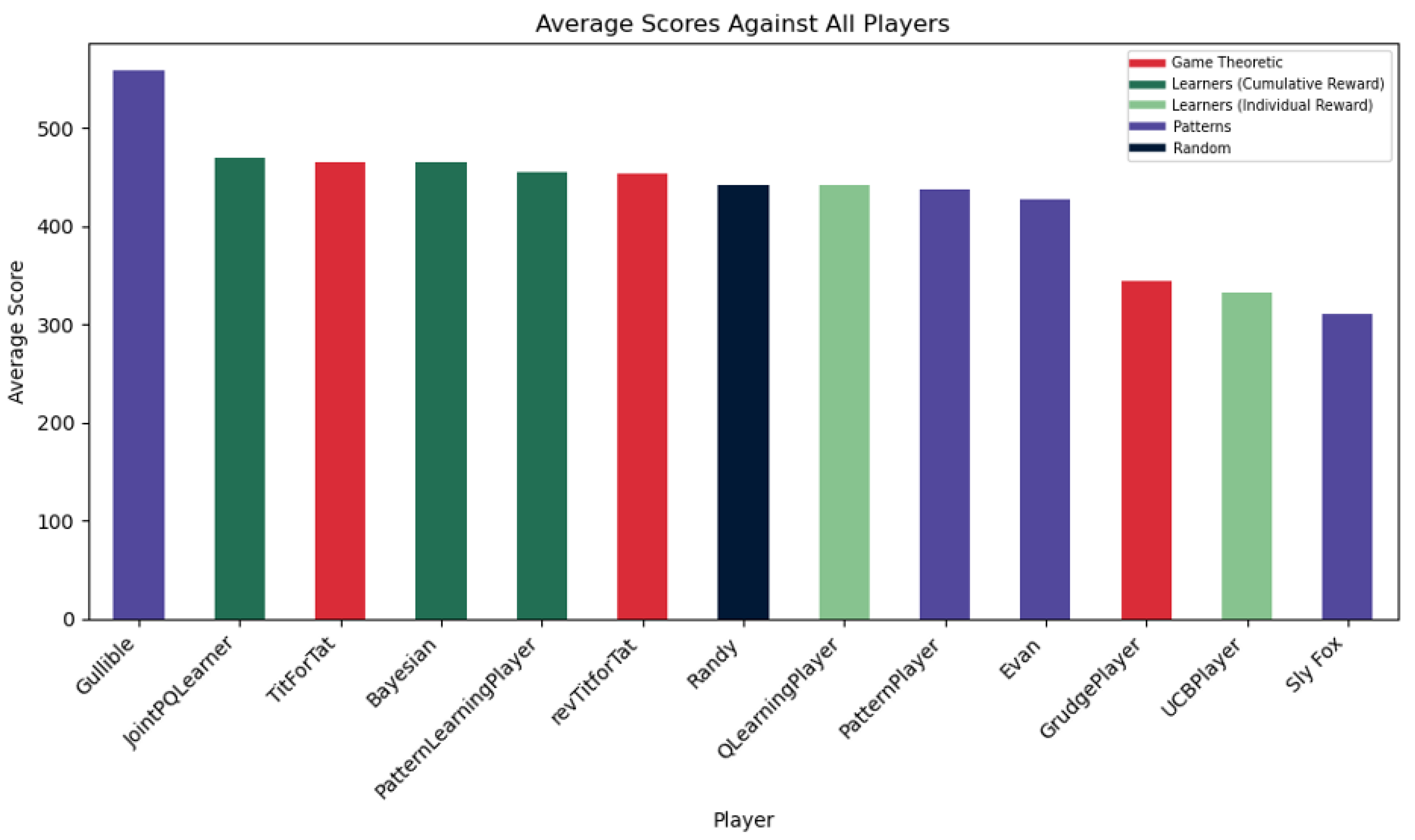
Figure 9.
Win Rates of Different Strategies
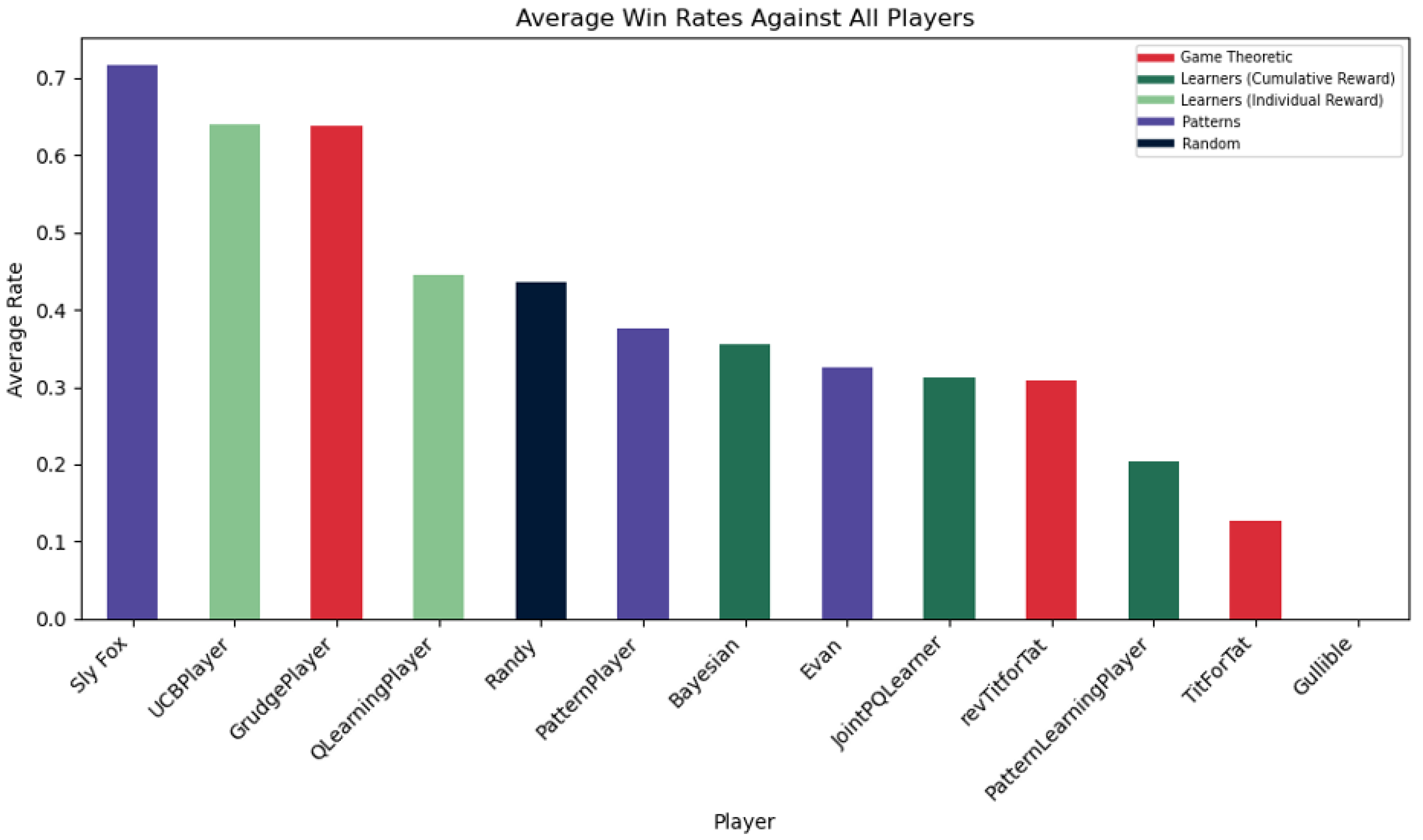
Figure 10.
CC Rates of Different Strategies
Disclaimer/Publisher’s Note: The statements, opinions and data contained in all publications are solely those of the individual author(s) and contributor(s) and not of MDPI and/or the editor(s). MDPI and/or the editor(s) disclaim responsibility for any injury to people or property resulting from any ideas, methods, instructions or products referred to in the content. |
© 2024 by the authors. Licensee MDPI, Basel, Switzerland. This article is an open access article distributed under the terms and conditions of the Creative Commons Attribution (CC BY) license (http://creativecommons.org/licenses/by/4.0/).
Copyright: This open access article is published under a Creative Commons CC BY 4.0 license, which permit the free download, distribution, and reuse, provided that the author and preprint are cited in any reuse.


