
Submitted:
19 July 2024
Posted:
22 July 2024
You are already at the latest version
Abstract
This study examines the aggregate consumption function of Saudi Arabia from 2000 to 2022, focusing on identifying key determinants of household consumption and evaluating the impacts of disposable income, household wealth, government expenditure, interest rates, and oil revenues. The research uses advanced econometric methods, including the Autoregressive Distributed Lag (ARDL) model and Johansen cointegration test, to analyze the relationships among these variables. The findings reveal that disposable income, household wealth, and government expenditure significantly and positively influence consumption, whereas interest rates show a negative correlation. Oil revenues also play a critical role, reflecting the country's economic reliance on oil. The study highlights the necessity for economic diversification to reduce the impact of oil price volatility on household income and consumption stability. The results offer crucial insights for policymakers, emphasizing the need for strategies that enhance household income and wealth, maintain robust public sector spending, and effectively manage interest rates. These findings also support the importance of consistent and predictable income sources for sustaining consumption. Additionally, this study suggests directions for future research, including developing sophisticated forecasting models to predict consumption trends and exploring other influencing factors such as demographic shifts and technological progress.
Keywords:
aggregate consumption
; government spending
; oil revenues
; interest rates Saudi Arabia
1. Introduction
Consumption stands as one of the two most crucial macroeconomic variables. Whatever happens to investment - whether it rises or falls - will not change the fact that consumption is the most significant component of the national income. Consumption accounts for about two-thirds of the GDP of a country. For both developed and developing countries, consumption is the most stable, leading, and predictable of the national income components. Thus, a clear understanding of the factors that keep consumption stable from decade to decade has a potential impact across a broad range of issues. That is why some macroeconomic theorists consider the consumption function the most important relationship in macroeconomic theory. Understanding the aggregate consumption function is pivotal for analyzing economic performance and policy effectiveness, particularly in economies undergoing significant structural changes. This study focuses on the aggregate consumption function of Saudi Arabia from 2000 to 2022, a period marked by profound economic transformations and policy initiatives, including the ambitious Vision 2030 plan aimed at diversifying the economy away from oil dependency.
Figure 1.
Saudi Household Consumption (2000–2022).
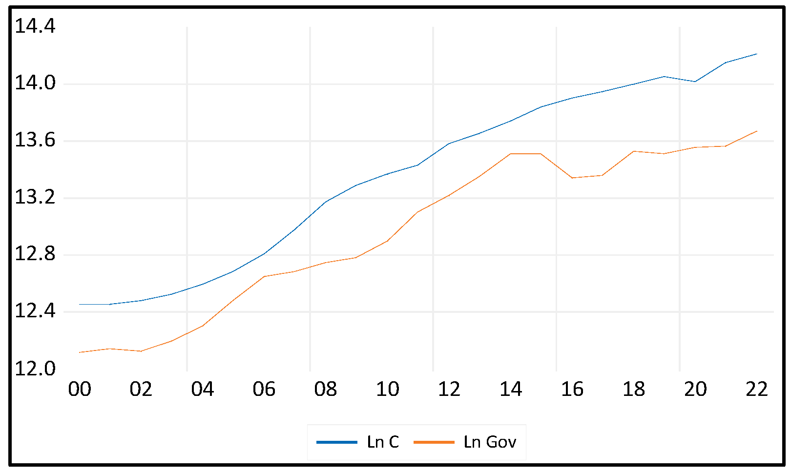
Figure 2.
Saudi Household Consumption & Government Expenditure (2000–2022).
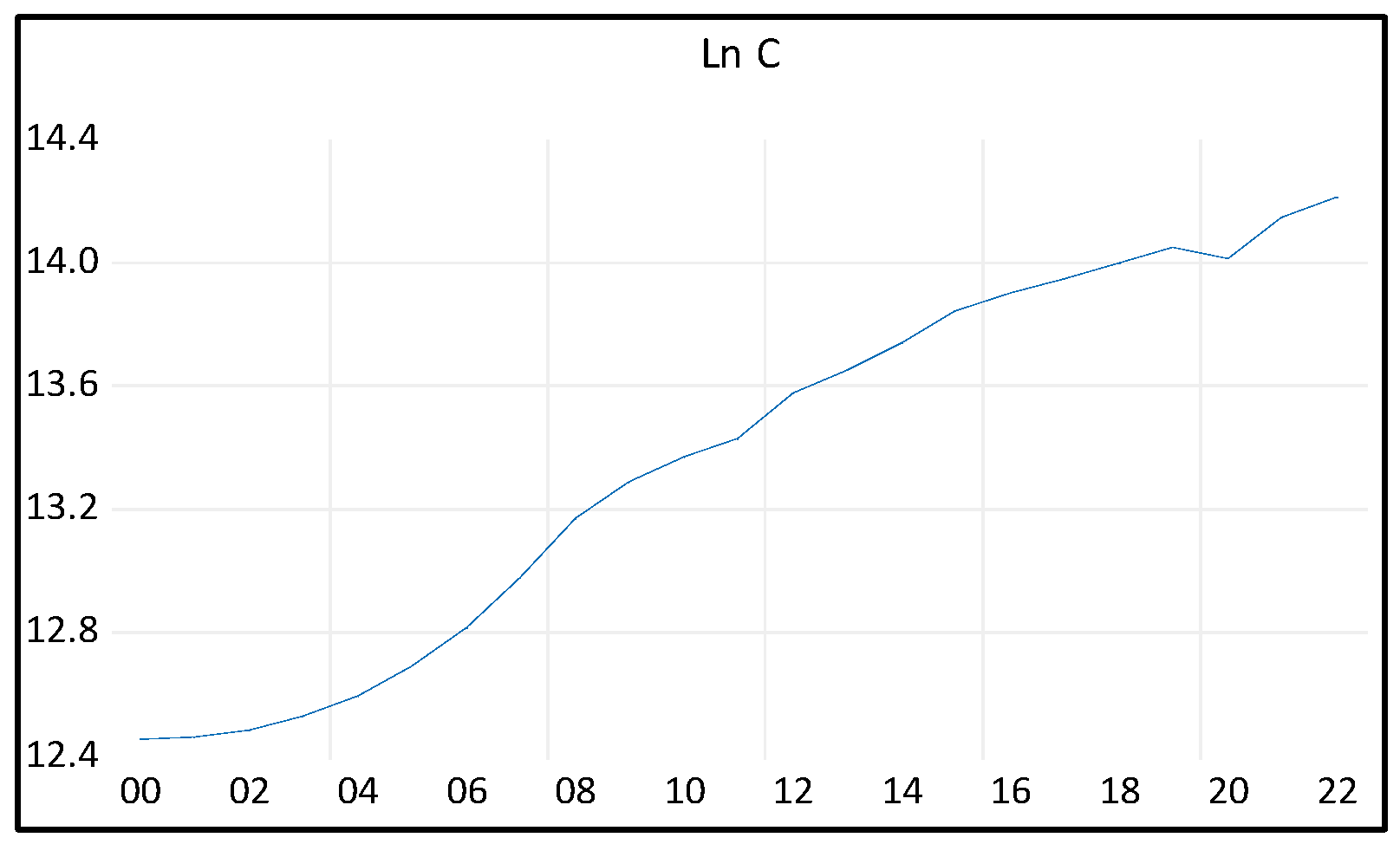
Figure 3.
Saudi Household Consumption & Disposal Income (2000–2022).
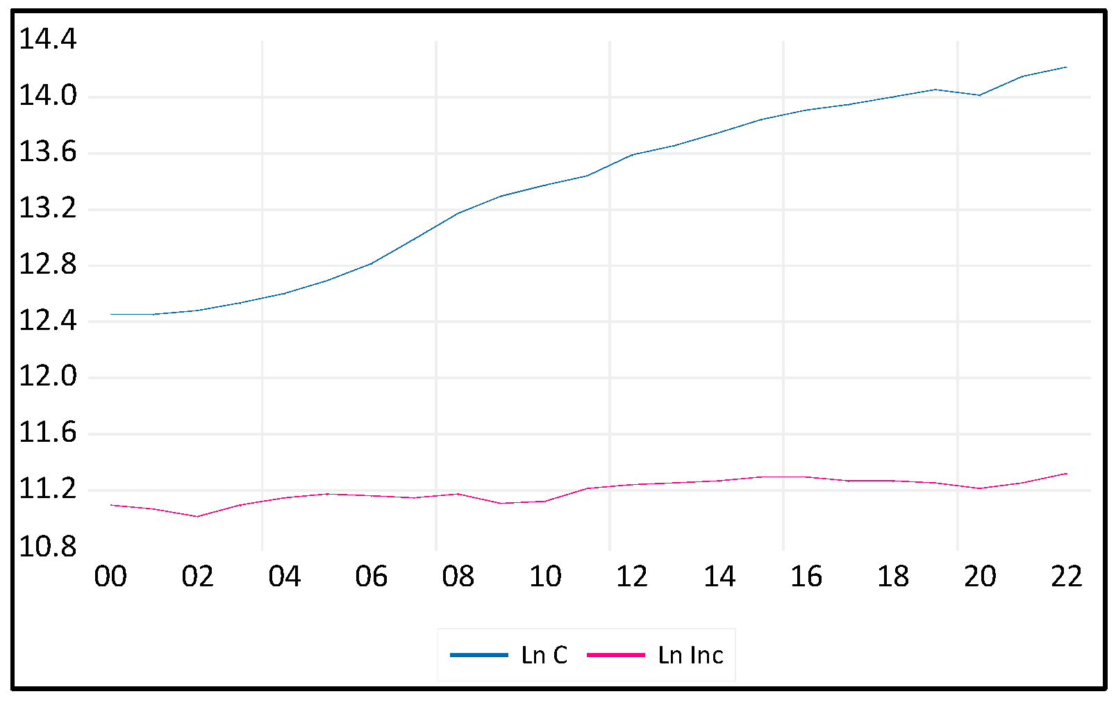
Figure 4.
Saudi Household Consumption & Oil Prices (2000–2022)**.
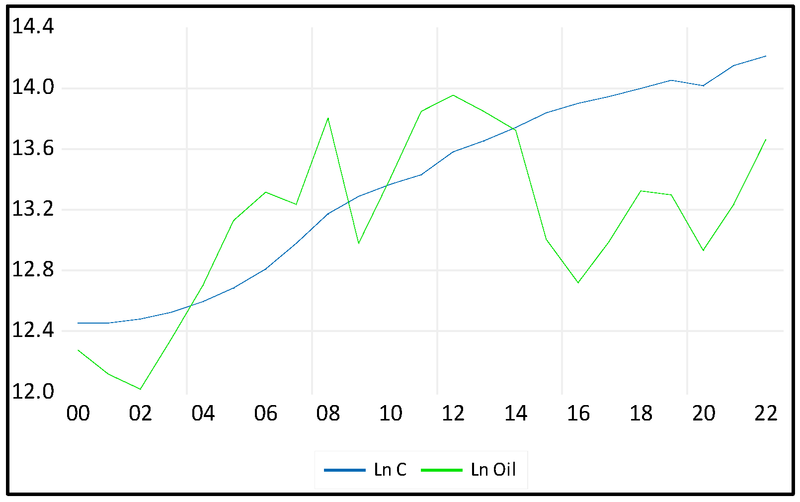
Figure 5.
Saudi Household Consumption & Interest Rates (2000–2022)*.
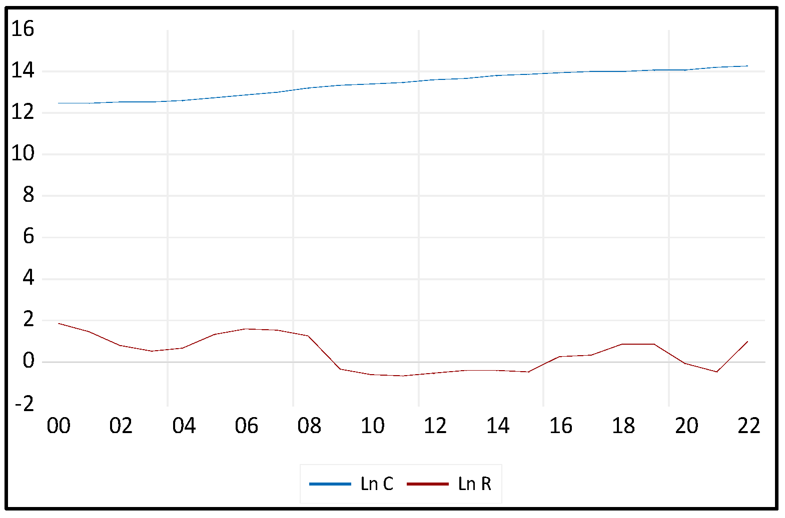
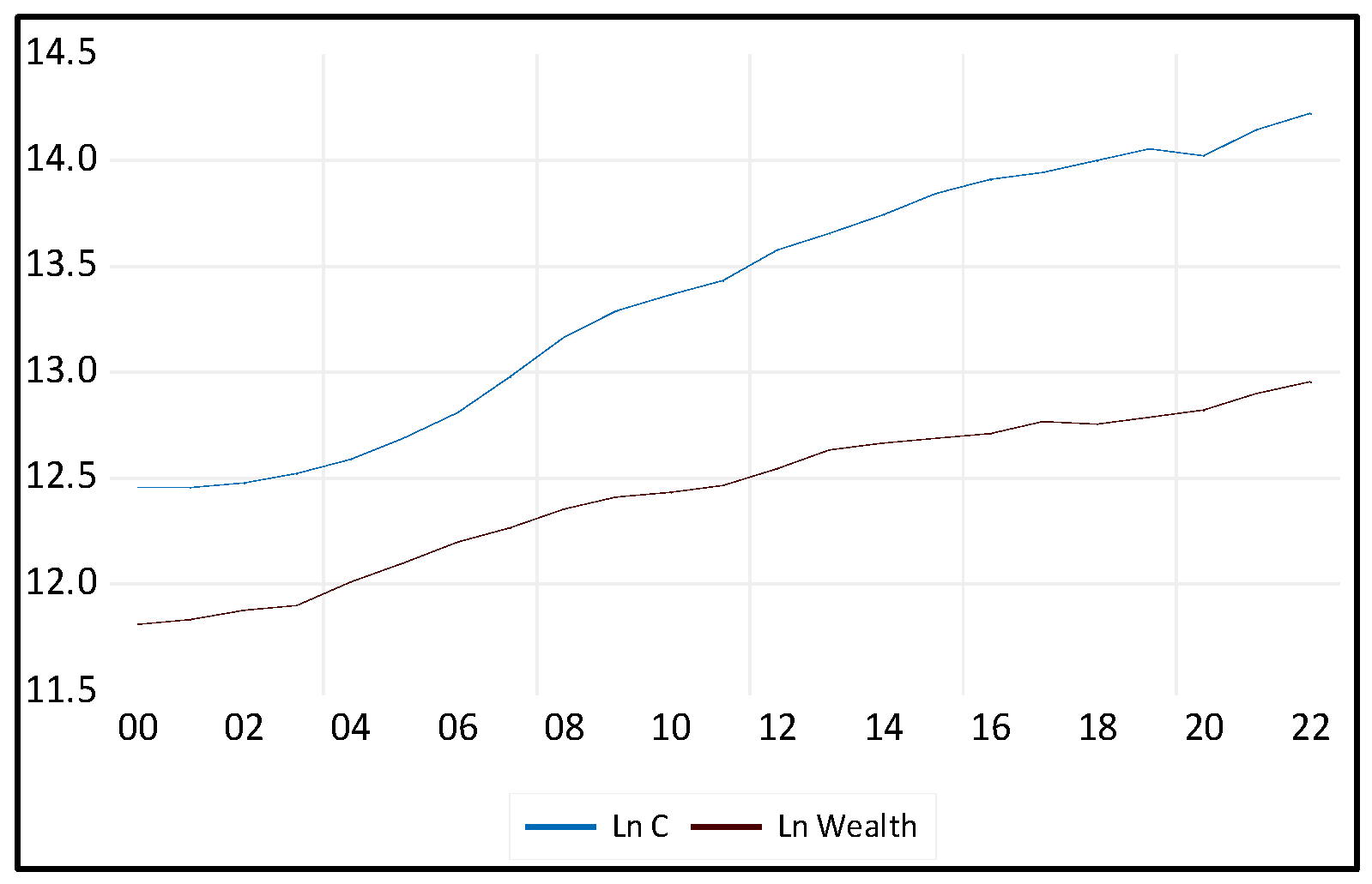
Figure 6.
Saudi Household Consumption & Household Wealth (2000–2022)*.
*unit: million, currency: Riyals. Source: Saudi Central Bank statistical reports. Statistical Report (sama.gov.sa). https://www.sama.gov.sa/en-us/economicreports/pages/report.aspx?cid=55 (accessed on 24 May 2024).
Unit: Million, Currency: Riyals. Budget allocation for fiscal year 1411/12 (1991) was amalgamated with the 1410/11 1(990) budget. In 2000, 2002, and 2004, Salaries of 13 months were paid. In 2010, The Surplus did not include expenditure on projects from the surplus account (Rls17057 Million). Moreover, it includes deposits (Rls 731 million) in the government's current account. Note: As of 1407/08 (1987), the kingdom's fiscal year begins on the 10th Capricorn of the Zodiac year. Up to 1405/06 (1985), the fiscal years covered the period from 1st Rajab to the end of Jumad II. Source: General Authority for Statistics. https://www.stats.gov.sa/en (accessed on 12 June 2024).
The figures above present the time series data for the natural logarithms of household consumption (Ln C) and government expenditure (Ln Gov); disposal income (Ln Inc); oil revenues (Ln Oil); interest rates (Ln R); household wealth (Ln Wealth) in Saudi Arabia from 2000 to 2022. Household consumption, government expenditure, oil revenues, and household Wealth show an upward trend over the period. This indicates that Saudi household consumption and other variables have generally increased. At the same time, interest rates in the same period exhibit considerable fluctuations without a clear long-term trend. The lack of a strong correlation between the two suggests that household consumption has been influenced by a broader set of factors beyond just interest rates. This underscores the complexity of the consumption function and the need for comprehensive models to understand the various determinants of household consumption.
Saudi Arabia's economy has historically relied heavily on oil revenues, influencing national income and consumption patterns. However, the volatility of global oil prices has posed challenges to economic stability and growth, necessitating a deeper understanding of the factors that drive consumption. The consumption function, which links aggregate consumption to various determinants such as disposable income, wealth, interest rates, government spending, and oil revenues, is a critical tool for this analysis.
This study aims to enhance the empirical understanding of the consumption function in Saudi Arabia by addressing the following key objectives: (1) identifying the primary determinants of household consumption, (2) analyzing the impact of economic policies and structural changes on consumption patterns, and (3) providing insights into the stability and dynamics of the consumption function over time.
Given the limited empirical literature on the aggregate consumption function in Saudi Arabia, particularly concerning the integration of structural breaks and policy impacts, this study fills a significant gap. Previous research has often relied on simple linear models, which may not adequately capture the complex interactions between variables in a rapidly changing economic environment. By employing advanced econometric techniques, this study provides a more nuanced and accurate estimation of the consumption function—Central Bank with additional support from the Saudi Central Authority for Statistics. The aim is to integrate the Saudi consumption function with several structural breaks in section 2: the oil-revenue shock, the housing mortgage estimation period, the Vision realization, and the post-vision periods. This, in turn, sharpens our findings over different periods. The consumption function provides insights into Saudi Arabia's income and wealth distribution and the government's tax policy until Vision 2030.
The findings of this research are expected to offer valuable insights for policymakers, economists, and stakeholders involved in economic planning and development. By understanding the determinants of consumption, policymakers can design more effective fiscal and monetary policies to stabilize and stimulate the economy. Additionally, insights into the consumption function can inform strategies for achieving sustainable economic growth and improving Saudi citizens' living standards.
This paper is structured as follows: Section 2 reviews the relevant literature on consumption functions globally and in Saudi Arabia. Section 3 outlines the theoretical framework and specifies the econometric models used in the analysis. Section 4 describes the data sources and methodology. Section 5 presents the empirical results and discusses their implications. Finally, Section 6 concludes the study and offers recommendations for future research.
2. Related Literature
2.1. Disposal Income
The phenomenon of total consumption is typically analyzed through the lens of the permanent income and life cycle theories. Keynes analyzed the functioning of the multiplier in implementing a stabilization policy. Based on the macroeconomic data, he observed a nonproportional connection between consumption and income during shorter time frames. According to Keynes' seminal work, an increase in income will result in a proportional expansion of consumer spending, albeit by a fraction of the initial income increase.
The aggregate consumption function of Saudi Arabia has been studied extensively in the context of various economic reforms, energy consumption, and economic diversification strategies. Given the country's unique economic structure, the consumption function especially gained significant attention, as it relies heavily on oil revenues. A micro-based life cycle consumption model for Saudi Arabia during the years 1970-2017 is estimated by Al Gahtani et al. (2019). The findings reveal a substantial impact of income on consumption, with a long-term marginal propensity to consume (MPC) ranging from 0.73 to 0.95. Similarly, wealth also plays a role in shaping consumption patterns, with an MPC of approximately 0.06.
Moreover, Al Moneef and Hasanov (2020) investigate the impact of fiscal spending on the Saudi economy, highlighting the relationship between fiscal policies, disposable income, and consumption. The findings indicate that the spending multiplier is more significant in the short term but decreases in the long term. Conversely, the capital spending multiplier is lower in the short term but increases in the long term. Moreover, a higher spending multiplier is observed during economic recessions, while it is deemed insignificant during economic expansions. Additionally, the multipliers identified in this study are slightly smaller than those reported in earlier research. However, Saudi Arabia has experienced significant socio-economic transformations over the past twenty years.
Consequently, the quality of life for most Saudi Arabian citizens has significantly improved, resulting in a considerable rise in household spending, especially for their children (Al-Banawi, 2014). Nevertheless, AlObaid (2021) analyzes the propensity variations based on income levels. The research reveals that the Citizen's Account Program (CAP) has led Saudi households to allocate an average of 20 halal for every one-riyal received. Accordingly, Saudi consumers will likely allocate 19.5% of their additional income towards non-durable goods, 25.5% towards semi-durable goods, and 16.8% towards services.
2.2. Household Wealth
The impact of wealth on consumption can vary significantly from the influence of income due to its strong connection with consumers' anticipations and changes in the worth of tangible and intangible assets. Al Gahtani et al. (2019) concluded that the responsiveness of consumption to changes in income and wealth, along with the projected immediate impacts of price and real interest rate, align with the burgeoning Saudi Arabian economy. The evidence suggests that a remarkably minor portion of the disparity in household net worth can be attributed to fluctuations in aggregate consumer spending (Lettau & Ludvigson, 2004). According to data from the United States, it is estimated that there is an immediate marginal propensity to consume approximately 2 cents for every $1 change in housing wealth in the next quarter (Carroll et al., 2006). Furthermore, it is projected that this effect will increase to around 9 cents in the long run. These findings indicate that the impact of housing wealth on consumption is significantly greater than that of stock wealth.
Nevertheless, compelling evidence suggests that fluctuations in housing market wealth significantly impact consumption patterns (Case et al., 2001). In developed nations, however, the housing market holds greater sway over consumption than the stock market. Conversely, Bernheim et al. (2001) concluded that wealth varies widely among similar households due to differences in preferences and risk tolerance. However, data from the Panel Study of Income Dynamics and the Consumer Expenditure Survey show little evidence that these factors affect wealth accumulation and consumption profiles. Regarding Consumption, growth demonstrates a positive correlation with financial literacy.
On the other hand, Jappelli and Padula's (2013) findings suggest a positive correlation between financial literacy and the anticipated consumption growth rate. This aligns with the notion that individuals with higher literacy levels in finance are more likely to have access to well-performing investment portfolios. However, Dack and Vasilev (2023) found that real interest rates have a significant inverse relationship with consumption. An elevation in the global real interest rate eventually intensifies the borrowing restriction and substantially reduces consumption for repayment (Yamada, 2023).
2.3. Interest Rates
The relationship between consumption and interest rates is pivotal in comprehending economic dynamics, impacting individual financial choices and macroeconomic strategies in Saudi Arabia. According to the principles of mainstream economics, when the interest rate increases, there is an anticipated impact on consumption (Dack & Vasilev, 2023). This is because the higher interest rate makes saving more attractive, as the potential reward for saving has increased. Conversely, borrowing money becomes significantly more costly, discouraging individuals from engaging in borrowing activities. As Weber (1970) mentioned, "It has been determined that under the assumptions we have made, interest rates play a crucial role in influencing aggregate consumption". The modification of aggregate consumption is influenced by the variations in consumption patterns across different age groups. Through numerical simulation, it has been observed that a reduction in the interest rate results in a significant increase in consumption in the short term, leading to a consumption boost (Kozlov, 2023). However, over time, as consumption gradually adapts to the new interest rate value, the magnitude of this boost diminishes. Hviid et al.'s (2017) findings indicate that the overall impact of the resulting liquidity changes on consumption is relatively modest. Nevertheless, it is important to note that certain vulnerable groups, including households with substantial debt and adjustable-rate mortgages, exhibit a significantly higher sensitivity to changes in interest rates. At the same time, Nordström (2020) concluded that the responsiveness of interest rates to changes in consumption growth has waned in the USA and Sweden, potentially because the zero lower bound restricts central banks. The most accurate representation of the relationship between consumption growth and short interest rates is to assume that it remains constant throughout the entire period. However, Auclert (2019) assessed the impact of redistribution on the transmission of monetary policy to consumption and concluded that there are three main channels through which aggregate spending is influenced when individuals with varying marginal propensities to consume experience income disparities; an interest rate exposure channel triggered by fluctuations in real interest rates is one of them. On the other hand, Jappelli & Padula (2013). Findings suggest a positive correlation between financial literacy and the anticipated consumption growth rate. This aligns with the notion that individuals with higher literacy levels in finance are more likely to have access to well-performing investment portfolios. However, Dack and Vasilev (2023) found that real interest rates have a significant inverse relationship with consumption. An elevation in the global real interest rate eventually intensifies the borrowing restriction and substantially reduces consumption for repayment (Yamada, 2023).
2.4. Oil Revenues
The interconnection between overall consumption and oil revenues holds significant importance for Saudi Arabia, an economy heavily relying on oil exports. Sultan & Haque's (2018) research delves into examining how oil exports affect economic growth and consumption expenditure in Saudi Arabia. The findings of this study reveal that the surge in oil revenues results in an elevation of disposable income, subsequently stimulating aggregate consumption. Likewise, Mahmood and Zamil (2019) explored how fluctuations in oil prices affect personal consumption levels. The study shows that oil price shocks significantly impact income levels, directly influencing aggregate consumption.
Moreover, Blazquez et al. (2020) examined the potential benefits of decreasing oil consumption in Saudi Arabia, including boosting oil revenues and enhancing overall economic productivity. These positive outcomes can indirectly contribute to promoting higher levels of aggregate consumption. At the same time, Hemrit and Benlagha (2018) investigated the influence of government spending, which is funded by oil revenues, on non-oil GDP and aggregate consumption. The findings indicate a favorable association between government expenditure and levels of consumption. Furthermore, Mezghani and Haddad (2017) explored the relationship between electricity consumption and economic growth, noting how oil revenues support higher energy consumption, boosting aggregate consumption.
Additionally, Hasanov (2019) revisits the theoretical framework for industrial electricity consumption, applying it to Saudi Arabia. The study provides empirical insights and future projections, showing how industrial energy consumption has evolved and what factors influence it. Moreover, Mikayilov and Darandary (2023) explored regional disparities in electricity demand and how these differences affect overall energy consumption in Saudi Arabia. The study provides a detailed analysis of electricity demand from 2000 to 2023, highlighting significant regional characteristics and their implications for national consumption. Likewise, Atalla et al. (2018) focus on the implications of gasoline pricing reforms on social welfare. The study presents a detailed quantitative analysis of gasoline demand and the effects of pricing policies, demonstrating their impact on consumption and economic welfare.
Nevertheless, oil price shocks impact various macroeconomic variables, including consumption, by altering oil revenues and, thus, household income (Hamdi & Sbia, 2013; Algaeed, 2017; Almutairi, 2020). Nevertheless, Alkhathlan and Javid (2015) and Alshehry and Belloumi (2015) linked oil consumption to carbon emissions and economic growth, highlighting the role of oil revenues in supporting aggregate consumption and overall economic activity. Furthermore, Alkhathlan and Javid (2013) concluded that the extended income elasticities of carbon emissions in the three models exhibit positivity and surpass their respective short-term income elasticities.
2.5. Government Expenditure
Saudi Arabia heavily relies on its petroleum reserves, which play a significant role in its economic landscape. These reserves contribute to approximately 87% of the nation's budget revenue, 42% of its Gross Domestic Product (GDP), and a substantial 90% of its export earnings (Haque et al., 2019). Eid (2015) examined the effects of government spending on the growth of non-oil GDP, illustrating how government expenditure shapes aggregate demand and consumption trends within the economy of Saudi Arabia. Mezghani and Haddad (2017), Mahmood and Zamil (2019), and Sultan and Haque (2018) concluded that increased government expenditure, especially during periods of high oil prices, significantly boosts aggregate consumption. Although Ahmad & Masan (2015) focused on Oman, it offers valuable insights into the influence of government spending on economic growth and consumption. These findings apply to understanding similar dynamics in Saudi Arabia. Mensi et al. (2017) investigated the unequal impacts of public and private investments on non-oil GDP, emphasizing the influence of government expenditure on overall demand and consumption patterns. Besides, Al-Yousif (2000) explored whether government spending promotes or inhibits economic growth and how this spending impacts aggregate consumption in Saudi Arabia. Moreover, Haque et al. (2019) examined the impact of oil production and government expenditure on human development in Saudi Arabia. Highlighted how increased government spending, funded by oil revenues, positively affects aggregate consumption and overall welfare.
The body of research concerning Saudi Arabia's aggregate consumption function demonstrates a notable scholarly focus on analyzing the effects of economic reforms and diversification strategies. Since 2015, the government has initiated energy price and fiscal reforms to enhance fiscal planning, public finance management, and budget execution and ultimately increase the efficiency of government expenditure (Hasanov et al., 2022). Blazquez et al. (2020b) employ a Dynamic Stochastic General Equilibrium (DSGE) model to evaluate the impact of economic reforms on Saudi Arabia's economy, emphasizing the dependency on oil revenues and the efforts towards economic diversification. The analyzed reforms significantly affect consumption patterns and overall economic stability.
3. Theoretical Framework
Key Determinants of Saudi Aggregate Consumption Function
To identify specific determinants of the Saudi aggregate consumption function, we must consider the unique economic, social, and institutional factors influencing consumption behavior in Saudi Arabia. Based on existing literature and economic theories, the primary determinant of consumption is disposable income, which is the income available to households after taxes and transfers.
where:
Ct= α + βYdt + ϵt
Ct: Consumption at time t
Ydt: Disposable income at time t
α: Autonomous consumption (when income is zero).
β: Marginal propensity to consume (MPC).
ϵt: Error term.
Household wealth (W), including financial assets, real estate, and other investments, significantly impacts consumption.
Ct = α + β1Ydt + β2Wt + ϵt
Interest rates (R) influence the cost of borrowing and the return on savings, affecting consumption decisions.
Ct = α + β1Ydt + β2Wt +β3Rt + ϵt
In Saudi Arabia, oil revenues (O) play a critical role in the economy and significantly influence national income and consumption.
Ct = α + β1Ydt + β2Wt +β3Rt + β4Ot + ϵt
Government spending (G) on social services, subsidies, and public sector wages can impact household consumption.
Ct = α + β1Ydt + β2Wt +β3Rt + β4Ot + β5Gt + ϵt
Ln Ct = α + β1 Ln Ydit + β2 Ln Wit +β3 Ln Rit + β4 Ln Oit +β5 Ln Git
4. Methodology
4.1. Data Sources and Variables
This study's data was obtained from the official Saudi Central Bank open portal data, the General Authority for Statistics, and the World Bank. The variables utilized were carefully defined using information obtained from the World Bank. The analysis was conducted using EViews 12 software, known for its flexibility and user-friendly features. This software effectively supported data management, visualization, and analysis, guaranteeing a thorough and efficient analytical procedure.
4.2. Definition of the Variables
Dependent Variable
Aggregate Consumption (C): The Gross Final Consumption Expenditure denoted by (C) is the dependent variable. It encompasses the total value of goods and services acquired by households, including durable products. This measure does not include the purchase of dwellings but does include imputed rent for owner-occupied dwellings. Furthermore, it covers government payments and fees for permits and licenses. Importantly, this indicator includes the expenditures of nonprofit institutions serving households, even if they are reported separately by the country.
Independent Variables
1. Disposable income, denoted by (Yd), is the amount of money households have available for spending and saving after income taxes have been accounted for. It is calculated as the gross income of households minus direct taxes, and it includes earnings from employment, self-employment, investments, and any other sources of income.
2. Household wealth, denoted by (W), is the total value of financial and nonfinancial assets owned by households minus their liabilities. This study measures household wealth using Real estate properties.
3. Interest rates, denoted by (R), refer to the cost of borrowing or the return on savings. Specifically, it is the proportion of a loan charged as interest to the borrower, typically expressed as an annual percentage of the loan amount.
4. Oil revenues, denoted by (O), refer to the income a country earns from oil extraction, production, and sale. This includes export revenues, domestic sales, taxes and royalties, and government participation.
5. Government spending, denoted by (G), includes public service, defense education, health, social security and welfare services, housing and community amenities, other community and social services, and economic services.
4.3. Econometric Methodology
This study employs various econometric techniques to address the challenges posed by time series data, causality, and cointegration. Furthermore, the Autoregressive Distributed Lag (ARDL) methodology is commonly employed in econometrics to estimate and analyze the enduring relationships between variables, particularly in the context of time series data analysis (Mohammed, 2024). This approach frequently simulates cointegration and dynamic connections among economic factors. Additionally, the model specification in the ARDL model, as opposed to traditional regression models, includes lagged values of both the dependent and independent variables to capture the evolution of the relationship over time. However, using differences helps to prevent the problem of false correlations caused by shared trends. However, it also risks overlooking the long-term equilibrium (cointegrating) connections that could be present between the levels of these variables. Various econometric methods can be employed for analysis, such as the dynamic ordinary least squares (DOLS) estimation technique, the Johansen cointegration test, and the error correction model (ECM). These approaches are well-suited for examining the long-term relationships, short-term dynamics, and causal links between variables of Saudi consumption function.
DOLS is a statistical technique used to estimate parameters in dynamic regression models that involve time series data with potential integration. MacKinnon et al. (1999) emphasized that the DOLS method is widely used to examine cointegrated time series.
The general formula for DOLS is:
where:
∆Yt = α + β1∆Xt + εt
∆It is the dependent variable at time t;
∆Xt is the independent variable(s) that exists at time t;
α is the intercept.
β is/are the coefficients of the independent variables;
εt is the error term at time t.
Furthermore, the Johansen cointegration test involves the estimation of a vector autoregressive (VAR) model followed by the conduction of likelihood ratio tests to assess the model's suitability. The equation for the Johansen cointegration test can be expressed as:
where:
Δyt = Πyt−1 + Γ1Δyt−1 + Γ2Δyt−2…….. + ΓpΔyt−p + ϵt
Δyt is the difference vector of time series variables at time t.
Π represents the matrix of cointegration coefficients.
Γi is the matrices of adjustment coefficients.
p is the lag length of the VAR model.
ϵt is the error term.
Besides, ECM is a theoretical framework utilized to examine the short-term and long-term interactions between variables in a cointegrated relationship. The core equation of ECM can be expressed as:
where:
∆Yt = α + β1(∆Yt − 1 − β2∆Xt − 1) + γ∆Xt + δ1∆Yt − 1 + δ2∆Xt − 1 + εt,
∆Yt: represents the short-term changes in the dependent variable at time "t,"
∆Xt: indicates the short-term variations in the independent variable(s) at time "t."
α: is the intercept term that signifies the constant effect on the dependent variable,
β1: measures the speed of the adjustment process in response to deviations from the long-term balance observed in the previous period.
β2: is the coefficient associated with the lagged difference in the independent variable(s) to adjust for deviations from the equilibrium condition.
γ: is the coefficient that represents the initial modification in the explanatory variable's coefficient, reflecting the direct impact of variations in the explanatory variable on the response variable. Additionally.
δ1: captures any persistence or autocorrelation through the coefficient of the lagged first difference in the dependent variable.
δ2: is a potential persistence or autocorrelation effect by including the lagged first difference coefficient within the independent variable(s).
εt: represents the error term signifying the unaccounted variability in the dependent variable at time "t."
For the analysis of the Saudi consumption function, the ECM can be specified to include the following components based on the critical determinants identified:
where:
Ct = α + β1∆Ydt + β2∆Wt + β3∆Rt + β4∆Ot + β5∆Gt + λECTt−1 + εt
∆Ct = change in aggregate consumption
∆Ydt = change in disposable income.
∆Wt = change in household wealth.
∆Rt = change in interest rates.
∆Ot = change in oil revenues.
∆Gt = change in government spending
λ = coefficient of the Error Correction Term (speed of adjustment).
ECTt−1 = lagged error correction term (deviation from long-term equilibrium).
εt = error term.
5. Analysis Results & Discussion
Table 1 presents the descriptive statistics for the variables, including mean, standard deviation (Std. Dev.), skewness, kurtosis, and the Jarque-Bera test for normality. Moreover, it provides the average ratio of the natural logarithm of Consumption from 2000 to 2022, roughly 13.36%, with a standard deviation of 0.62. The average Ln disposal income is approximately 11.2%, with a standard deviation of 0.05. Taken together, these statistics indicate that the model is predominantly stable. The p-values of Jarque-Bera indicate that the data follow a normal distribution (i.e. all p-values > 0.05).
The correlation matrix in Table 2 indicates that wealth shows the highest positive correlation with household consumption (0.993), followed by government expenditure (Gov) (0.985), disposal income (Inc) (0.881), and Oil revenues (0.561). Nevertheless, Table 2. indicates the negative relationship between interest rates and household consumption (-0.536). These results are important for understanding the composition of Saudi aggregate consumption function and providing a comprehensive overview of the relationships between variables.
Based on the findings in Table 3, the unit root (ADF) test indicates that all series displayed non-stationarity at a significance level of 0.05, as evidenced by the p-values. Failure of the t-statistics for the ADF test of the variables C, Gov, Inc, Oil, R, and Wealth to exceed the critical values at the 5% level implies non-stationarity in their level forms. Following the first difference, it was observed that the variables C, Gov, Inc, and Oil became stationary, with a p-value less than 0.05. However, the variables R and Wealth became stationary after following the second difference with a p-value less than 0.05.
Table 4. includes several factors such as log-likelihood (LogL), sequential modified (LR), Final Prediction Error (FPE), Akaike Information Criterion (AIC), Schwarz information criterion (SC), and Hannan–Quinn Information Criterion (HQ), which assist in identifying the optimal lag order for the VAR model. Upon examination of Table 4, it is clear that lag two is the most suitable option for a VAR model, as indicated by asterisks in the LR, FPE, AIC, SC, and HQ columns.
5.1. Cointegration Test Results
Cointegration analysis is crucial in examining stable relationships among Ln C, Ln Gov, Ln Inc, Ln Oil, Ln R, and Ln wealth over time. The Akaike Information Criterion (AIC) and Schwarz Criterion (SC) were employed to identify the lag length that best suits the model. These criteria were instrumental in selecting the model and were calculated based on the estimation of an unconstrained vector autoregressive model using the first differences of the variables. The results of the analysis reveal that the most suitable lag length for the model is two. Furthermore, Table 5 demonstrates a significant cointegration equation at the 5% level.
Given that all variables are integrated in the same order, the Johansen Cointegration test was conducted, and the findings are presented in Table 5. The analysis revealed that the trace value surpasses the critical value, indicating the presence of five Cointegration equations at a significance level of 5 per cent. Additionally, the maximum eigenvalue suggests the existence of four Cointegration equations.
The study examines the short-term model by incorporating the lag in Error Correction Term (ECT) as an independent variable. According to Table 6, the presence of a negative sign and the statistical significance of ECT (-1) suggest that adjustments to the model are feasible. The coefficient for ECT (-1) is 0.592, indicating the speed at which the model adjusts towards equilibrium. Likewise, Table 7 confirms the stationarity of ECT at the level (i.e., rejecting H0). Therefore, cointegration for the long-term relationships among the model variables is evident (Prob. = 0.000 < 0.05). Based on Table 6, it is evident that government expenditure, disposal income, and wealth positively influence long-term Saudi household consumption. Conversely, on average, oil revenues and interest rates negatively influence all else being equal. In conclusion, the null hypothesis of no cointegration is refuted in favor of the alternative hypothesis, suggesting a cointegration relationship within the model.
According to the findings presented in Table 7, the adjusted R-square value of 92% indicates a good fit for the cointegration model. At the same time, the F-statistics value represents the long-run cointegration relationship among variables under study at the significant level of 5% (F = 27.11, P-value = 0.000 < 0.05). Moreover, the cointegration equation shoes negative coefficient (-0.551) at the significant level of 5% (p-value = 0.000 < 0.05) indicate cointegration. Hence, the existence of cointegration indicates a long-term connection among the variables in the model.
5.2. Results of Granger-Causality Tests
Table 9 illustrates the causal relationship among the variables under investigation in this study as follows:
First: INC → C The rejection of the null hypothesis (H0) by the C test suggests a causal relationship. This signifies a statistically significant unidirectional causal link between INC and C, suggesting that variations in disposable income can result in significant fluctuations in household consumption in Saudi Arabia.
Second: Wealth → C, the null hypothesis (H0) has been rejected, providing evidence for a causal relationship. It was found that wealth significantly impacts Saudi households' consumption, thus establishing a unidirectional causal relationship between wealth and C. This suggests that fluctuations in wealth have a considerable influence on the Saudi aggregate consumption function.
Third: R → C, the null hypothesis (H0) is rejected, indicating the presence of a causal relationship. Interest rates demonstrate a statistically significant unidirectional causal association with C. Variations in R significantly influence household consumption in Saudi Arabia.
Fourth: Oil → C, rejection of H0 (causality relationship exists). A significant unidirectional causal link can be observed between the oil revenues and C. Implying variations in the trade balance have a noteworthy effect on Saudi household consumption.
Fifth: Gov → C, rejection of H0 (the causality relationship exists) suggesting a unidirectional causal link between the Saudi government expenditure and C. Accordingly, fluctuations in Gov have variations in Saudi aggregate consumption.

Table 8.
Granger causality tests.
| Null Hypothesis (H0) | F-Statistic | prob | Causality (H1) |
|---|---|---|---|
| INC → C | 0.18 | 0.84 | Yes |
| Wealth → C | 17.71 | 9 | Yes |
| R → C | 0.012. | 0.99 | Yes |
| Oil → C | 1.79 | 0.2 | Yes |
| Gov → C | 2.97 | 0.08 | Yes |
5.3. Discussion of the Results
The analysis of the aggregate consumption function in Saudi Arabia from 2000 to 2022 provides significant insights into household consumption dynamics in the context of an oil-dependent economy undergoing substantial socio-economic transformations. The empirical results suggest that household wealth, government spending, disposable income, and oil revenues significantly influence overall consumption patterns in Saudi Arabia. More specifically, the strong relationship between household wealth and consumption highlights the crucial role of financial and property assets in stimulating consumer expenditure.
The correlation matrix in Table 2 reveals that wealth exhibits the strongest positive correlation with household consumption (0.993). This finding suggests that financial and nonfinancial wealth is pivotal in shaping aggregate consumption in Saudi Arabia. Furthermore, the results of the long-term relationship analysis suggest that there are consistent and stable connections between wealth and household consumption in Saudi Arabia and consistent with (Al Gahtani et al., 2019; Lettau & Ludvigson, 2004; Paiella & Pistaferri, 2017). Consumption exhibits enduring reactions to disturbances, indicating that the long-run impact of wealth is notably more significant than its immediate impact. However, Jappelli and Pistaferri (2010) indicated that MPC falls within the range of 0.5 to 0.9. This result implies high confidence in the Saudi economy, as expectations held by individuals are critical factors that influence their choices, and most economic models prioritize the role of expectations concerning asset prices, future income, and individual life expectancy.
Government spending has been identified as a key factor in determining consumption, underscoring the important role of public sector expenditure in stimulating household income and, in turn, consumption. The analysis findings reveal a strong positive correlation between government expenditure and household consumption in Saudi Arabia, as evidenced by the remarkably significant positive value of the coefficient for Ln Gov (0.985). Hence, government expenditure significantly impacted Saudi consumption in this time frame. This result uncovers the generous spending of the Saudi government for its people, especially after 2008 (i.e. Vision 2030). This finding aligns with Al Moneef and Hasanov (2020), who emphasized the short-term and long-term effects of fiscal spending on the Saudi economy.
The relationship between disposable income and consumption plays a crucial role in conventional consumption theories, particularly in the Keynesian consumption function and the Permanent Income Hypothesis (PIH). The results of this research validate these theories, showing that a rise in disposable income results in an increase in consumer expenditure. The findings in this study corroborate the Keynesian view by showing a highly positive correlation (0.881) between disposable income and consumption in Saudi Arabia. This means that as households experience an increase in their disposable income, they tend to allocate a significant portion of this additional income to consumption, boosting overall economic activity. In Saudi Arabia, the study's results indicate that households' consumption patterns respond positively to changes in disposable income, suggesting that increases in permanent income (through stable economic growth and consistent income policies) would lead to sustained increases in consumption. This aligns with the PIH, emphasizing that stable and predictable income sources are crucial for steady consumption growth. Likewise, the empirical analysis reflects elements of the LCH, where increases in disposable income, particularly during prime earning years, result in higher consumption. This behavior indicates households optimizing their consumption patterns to maintain a stable standard of living throughout their lives.
On the other hand, understanding the positive influence of disposable income on consumption has significant policy implications. Policymakers in Saudi Arabia can leverage this relationship by implementing policies that enhance disposable income, such as tax cuts, subsidies, or direct cash transfers. Additionally, efforts to ensure stable and predictable income growth, such as through economic diversification and job creation, can help sustain consumption. Additionally, welfare systems and initiatives to ensure financial security during economic hardship can help mitigate drastic decreases in consumer spending, ultimately contributing to economic stability. It is crucial to uphold solid disposable income levels to bolster consumer trust and drive economic expansion.
Oil revenues, as expected, profoundly impact consumption patterns in Saudi Arabia. The country's heavy reliance on oil exports means that fluctuations in oil prices directly affect household income and consumption. Studies by Sultan and Haque (2018) and Mahmood and Zamil (2019) have documented the significant effects of oil price shocks on disposable income and consumption, highlighting the sensitivity of the Saudi economy to global oil market dynamics.
The analysis also revealed a negative relationship between interest rates and consumption. Higher interest rates increase the cost of borrowing and incentivize savings, reducing consumer spending. This inverse relationship is in line with mainstream economic theories and the findings of Dack and Vasilev (2023), who examined the effects of interest rates on consumption in different economic contexts.
During the period being examined, notable policy changes occurred, such as the introduction of the Saudi Vision 2030 program, which seeks to reduce the economy's reliance on oil. These fundamental alterations have consequences for how people spend their money. The strong relationship between government spending and consumption during this period indicates that investments made by the public sector in areas like social welfare, infrastructure, and subsidies have played a vital role in maintaining household spending levels.
The cointegration analysis confirmed the long-term stability of the relationships between the key determinants and aggregate consumption. The existence of a cointegration relationship implies that despite short-term fluctuations, the determinants of consumption move together in the long run, ensuring a stable consumption function for policy analysis and forecasting.
In conclusion, this study enhances the understanding of the aggregate consumption function in Saudi Arabia, providing a robust framework for analyzing the determinants of household consumption. The findings underscore the importance of disposable income, household wealth, government expenditure, interest rates, and oil revenues in shaping consumption patterns. By leveraging these insights, policymakers can design targeted interventions to sustain and enhance consumption, fostering long-term economic growth and stability.
6. Conclusions
This study provides a comprehensive analysis of the aggregate consumption function in Saudi Arabia from 2000 to 2022, offering valuable insights into the factors influencing household consumption in an oil-dependent economy. The findings highlight the critical roles of disposable income, household wealth, government expenditure, interest rates, and oil revenues in shaping consumption patterns. The study reaffirms traditional consumption theories, demonstrating that increases in disposable income significantly boost consumer spending. This positive relationship underscores the importance of policies enhancing household income to sustain consumption growth. Moreover, wealth drives consumption, particularly in financial assets and real estate. The positive correlation between wealth and consumption suggests that policies fostering asset accumulation can substantially impact consumer spending.
Furthermore, government spending on social services, infrastructure, and subsidies significantly influences household consumption. The positive impact of government expenditure highlights the importance of sustained public sector investments to support household income and consumption. However, oil price and revenue fluctuations profoundly affect disposable income and consumption in an oil-dependent economy. The study emphasizes the need for economic diversification to mitigate the volatility associated with oil revenues and ensure stable income growth. The negative relationship between interest rates and consumption indicates that higher borrowing costs deter consumer spending. This finding suggests that managing interest rates is crucial for balancing savings and consumption to stabilize the economy.
Policy Implications
The results of this study have several implications for policymakers in Saudi Arabia. Policies to increase disposable income, such as tax cuts, wage increases, and direct cash transfers, can significantly boost consumption and drive economic growth. Policymakers should focus on sustaining household income through diversified economic activities and stable public sector investments. Given the significant impact of oil revenues on consumption, efforts to stabilize oil income and invest in alternative revenue streams are essential. Also, managing interest rates to balance encouraging savings and boosting consumption is crucial for economic stability. Besides, encouraging asset ownership and investment in financial markets can enhance household wealth, thereby increasing consumer spending. Policies that promote real estate development and financial market participation are particularly beneficial.
Nevertheless. continued investment in social services, infrastructure, and subsidies is essential for supporting household consumption. Policymakers should ensure that government expenditure remains robust, especially during economic downturns. On the other hand, reducing the economy's reliance on oil revenues through diversification initiatives is crucial for achieving stable and sustainable income growth. Diversification can mitigate the adverse effects of oil price fluctuations on household consumption. In addition, balancing interest rates to encourage savings and consumption is essential for economic stability. Policymakers should consider the broader economic impact of interest rate changes on consumer spending.
Limitations and Future Research Directions
While this study provides significant insights into the determinants of aggregate consumption in Saudi Arabia, it is essential to acknowledge its limitations and the need for further research. Addressing these limitations and exploring the suggested future research directions can deepen the understanding of consumption behavior and inform more effective economic policies. Modelling constraints regarding the assumption of linearity in the consumption function might need to be more accurate in the complex relationships among the variables. Non-linear models or other advanced econometric techniques could provide a more nuanced understanding. The distinctive economic structure of Saudi Arabia, which heavily depends on oil revenues, suggests that the results may only apply to some countries with varying economic frameworks. Furthermore, the study may need to fully capture the impact of unobserved factors such as consumer confidence, cultural influences, and changes in household preferences, which can also affect consumption behavior.
Further research could explore the impact of other factors, such as demographic changes, technological advancements, and global economic conditions, on consumption patterns in Saudi Arabia. Additionally, examining the effectiveness of specific policy measures in enhancing disposable income and household wealth could provide deeper insights into optimizing consumption growth. Moreover, future studies could incorporate additional variables such as consumer confidence indices, employment rates, and demographic factors (e.g., age distribution and urbanization) to analyze consumption patterns comprehensively. Future research could also explore panel data analysis, combining cross-sectional and time-series data to account for regional differences and capture more detailed consumption behaviors. Cross-country analyzes could also show how different economic structures and policy environments influence consumption functions. Eventually, future research should focus on developing robust forecasting models for the Saudi consumption function to predict future consumption patterns better and inform economic policy.
Institutional Review Board Statement
Not applicable.
Data Availability Statement
The data presented in this study are available on request from the corresponding author.
Conflicts of Interest
The author declares no conflict of interest.
References
- Saudi Central Bank statistical reports. Statistical Report (sama.gov.sa). https://www.sama.gov.sa/en-us/economicreports/pages/report.aspx?cid=55.
- General Authority for Statistics. https://www.stats.gov.sa/en.
- Al Gahtani, G., Bollino, C. A., Bigerna, S., & Pierru, A. (2019). Estimating the Household Consumption Function in Saudi Arabia. Discussion Papers No. ks-2019-dp50). Retrieved from https://www. kapsarc. org/research/publications/estimating-the-household-consumption-function-in-saudi-arabia.
- Al Moneef, M., & Hasanov, F. (2020). Fiscal multipliers for Saudi Arabia revisited. King Abdullah Petroleum Studies and Research Center: Riyadh, Saudi Arabia.
- Al-Banawi, N. (2014). The proportion of expenditure on children to family's income in Saudi Arabia. International Journal of Business and Economic Development (IJBED), 2(3).
- Lettau, M., & Ludvigson, S. C. (2004). Understanding trend and cycle in asset values: Reevaluating the wealth effect on consumption. American economic review, 94(1), 276-299. [CrossRef]
- Christopher D. Carroll, Misuzu Otsuka, and Jirka Slacalek (2006). How large is the housing wealth effect?-a new approach: NBER Working Paper No. 12746 December 2006.
- Karl E. Case John M. Quigley Robert J. Shiller (2001). COMPARING WEALTH EFFECTS: THE STOCK MARKET VERSUS THE HOUSING MARKET. Working Paper 8606NATIONAL BUREAU OF ECONOMIC RESEARCH 1050 Massachusetts Avenue Cambridge, MA 02138 November 2001 http://www.nber.org/papers/w8606.
- Bernheim, B. D., Skinner, J., & Weinberg, S. (2001). What accounts for the variation in retirement wealth among US households? American Economic Review, 91(4), 832-857. [CrossRef]
- Hasanov, F. J., Alkathiri, N., Alshahrani, S. A., & Alyamani, R. (2022). The impact of fiscal policy on non-oil GDP in Saudi Arabia. Applied Economics, 54(7), 793–806. [CrossRef]
- Dack, K., & Vasilev, A. (2023). How Do Interest Rates Effect Consumption in the UK?. Advances in Business and Management, 77. [CrossRef]
- Hviid, S. J.; Kuchler, Andreas (2017): Consumption and savings in a low interest-rate environment, Danmarks National bank Working Papers, No. 116, Danmarks National bank, Copenhagen.
- Martin Nordström (2020). Consumption and the interest rate – A changing dynamic? Applied Economics, 52:51, 5564-5578. [CrossRef]
- Auclert, Adrien. (2019). "Monetary Policy and the Redistribution Channel." American Economic Review, 109 (6): 2333–67. [CrossRef]
- Jappelli, T., & Padula, M. (2013). Consumption growth, the interest rate, and financial literacy.
- Yamada, H. (2023). Financial Integration, Excess Consumption Volatility, and the World Real Interest Rate (No. HIAS-E-133).
- Weber, W. E. (1970). The effect of interest rates on aggregate consumption. The American Economic Review, 60(4), 591–600.
- Kozlov, R. (2023). The Effect of Interest Rate Changes on Consumption: An Age-Structured Approach. Economies, 11(1), 23. [CrossRef]
- Hviid, S. J.; Kuchler, Andreas (2017): Consumption and savings in a low interest-rate environment, Danmarks National bank Working Papers, No. 116, Danmarks National bank, Copenhagen.
- Sultan, Z. A., & Haque, M. I. (2018). Oil exports and economic growth: Empirical evidence from Saudi Arabia. International Journal of Energy Economics and Policy, 8(5), 281-287.
- Mahmood, H., & Zamil, A. (2019). Oil price and slumps affect personal consumption in Saudi Arabia. International Journal of Energy Economics and Policy, 9(4), 12-15. [CrossRef]
- Blazquez, J., Hunt, L. C., Manzano, B., & Pierru, A. a(2020). The value of saving oil in Saudi Arabia. Economics of Energy & Environmental Policy, 9(1), 207-222.
- Hemrit, W., & Benlagha, N. (2018). The impact of government spending on non-oil-GDP in Saudi Arabia (multiplier analysis). International Journal of Economics and Business Research, 15(3), 350-372.
- Mezghani, I., & Haddad, H. B. (2017). Energy consumption and economic growth: An empirical study of the electricity consumption in Saudi Arabia. Renewable and Sustainable Energy Reviews, 75, 145-156. [CrossRef]
- Hasanov, F. (2019). Theoretical Framework for Industrial Electricity Consumption Revisited (No. ks--2019-dp66).
- Mikayilov, J., & Darandary, A. (2023). Modelling and Projecting Regional Electricity Demand for Saudi Arabia (No. ks--2023-mp01). King Abdullah Petroleum Studies and Research Center. [CrossRef]
- Atalla, T. N., Gasim, A. A., & Hunt, L. C. (2018). Gasoline demand, pricing policy, and social welfare in Saudi Arabia: A quantitative analysis. Energy policy, 114, 123-133. [CrossRef]
- Hamdi, H., & Sbia, R. (2013). Dynamic relationships between oil revenues, government spending and economic growth in an oil-dependent economy. Economic Modelling, 35, 118-125. [CrossRef]
- Algaeed, A. H. (2017). The Effects of Asymmetric Oil Price Shocks on the Saudi Consumption: An Empirical Investigations. International Journal of Energy Economics and Policy, 7(1), 99–107.
- Almutairi, N. (2020). The effects of oil price shocks on the macroeconomy: Economic growth and unemployment in Saudi Arabia. OPEC Energy Review, 44(2), 181-204. [CrossRef]
- Alkhathlan, K., & Javid, M. (2015). Carbon emissions and oil consumption in Saudi Arabia. Renewable and Sustainable Energy Reviews, pp. 48, 105–111. [CrossRef]
- Alkhathlan, K., & Javid, M. (2013). Energy consumption, carbon emissions and economic growth in Saudi Arabia: An aggregate and disaggregate analysis. Energy policy, 62, 1525-1532. [CrossRef]
- Alshehry, A. S., & Belloumi, M. (2015). Energy consumption, carbon dioxide emissions and economic growth: The case of Saudi Arabia. Renewable and Sustainable Energy Reviews, 41, 237-247. [CrossRef]
- Haque, Mohammad Imdadul/Khan, Md Riyazuddin (2019). Role of oil production and government expenditure in improving human development index: evidence from Saudi Arabia. In: International Journal of Energy Economics and Policy 9 (2), S. 251 - 256. [CrossRef]
- Eid, A. G. (2015, November). Budgetary institutions, fiscal policy, and economic growth: The case of Saudi Arabia. In Economic Research Forum Working Paper (No. 965).
- Ahmad Hassan Ahmad & Saleh Masan (2015). Dynamic relationships between oil revenue, government spending and economic growth in Oman. International Journal of Business and Economic Development Vol. 3 Number 2.
- Walid Mensi, Syed Jawad Hussain Shahzad, Shawkat Hammoudeh, Khamis Hamed Al-Yahyaee (2017). Asymmetric impacts of public and private investments on the non-oil GDP of Saudi Arabia, International Economics, Volume 156. [CrossRef]
- Al-Yousif, Y. K. (2000). Do Government Expenditures Inhibit or Promote Economic Growth: Some Empirical Evidence from Saudi Arabia. The Indian Economic Journal, 48(2), 92–96. [CrossRef]
- Blazquez, Jorge & Galeotti, Marzio & Manzano, Baltasar & Pierru, A. & Pradhan, Shreekar. b(2020). Analysing the Effects of Saudi Arabia's Economic Reforms Using a Dynamic Stochastic General Equilibrium Model.
- Ramady, M. A. (2009). EXTERNAL AND I! \i'TERNAL DETERMINANTS OF INFLATION: A CASE STUDY OF SAUDI ARABIA.
- Mohammed, M. G. A. (2024). Analysing GDP Growth Drivers in Saudi Arabia: Investment or Consumption: An Evidence-Based ARDL-Bound Test Approach. Sustainability, 16(9), 3786. [CrossRef]
- MacKinnon, J.G.; Haug, A.A.; Michelis, L. Numerical Distribution Functions of Likelihood Ratio Tests for Cointegration. J. Appl. Econom. 1999, 14, 563–577. [CrossRef]
- Jappelli Tullio, and Luigi Pistaferri. 2010. “The Consumption Response to Income Changes”, Annual Review of Economics 2: 479–506. www.annualreviews.org. [CrossRef]
- Paiella, M., & Pistaferri, L. (2017). Decomposing the wealth effect on consumption. Review of Economics and Statistics, 99(4), 710-721. [CrossRef]
Table 1.
Descriptive Statistics (Common Sample).
| Ln C | Ln Gov | Ln Inc | Ln Oil | Ln R | Ln Wealth | |
|---|---|---|---|---|---|---|
| Mean | 13.36 | 12.97 | 11.2 | 13.13 | 0.48 | 12.43 |
| Median | 13.43 | 13.1 | 11.21 | 13.24 | 0.56 | 12.47 |
| Maximum | 14.21 | 13.67 | 11.32 | 13.95 | 12.02 | 12.69 |
| Minimum | 12.46 | 12.12 | 11.01 | 12.02 | -0.63 | 11.81 |
| Std | 0.62 | 0.55 | 0.08 | 0.57 | 0.83 | 0.37 |
| Skewness | -0.24 | -0.34 | -0.34 | -0.4 | 0.12 | -0.39 |
| Kurtosis | 1.57 | 1.62 | 2.22 | 2.27 | 1.61 | 1.84 |
| Jarque-Bera | 2.18 | 2.25 | 1.2 | 1.11 | 1.9 | 1.85 |
| Probability | 0.34 | 0.33 | 0.45 | 0.57 | 0.39 | 0.4 |
Table 2.
Correlation Matrix.
| Ln C | Ln Gov | Ln Inc | Ln Oil | Ln R | Ln Wealth | |
|---|---|---|---|---|---|---|
| Ln C | 1 | |||||
| Ln Gov | 0.99 | 1 | ||||
| Ln Inc | 0.88 | 0.91 | 1 | |||
| Ln Oil | 0.56 | 0.63 | 0.62 | 1 | ||
| Ln R | -0.54 | -0.55 | -0.39 | -0.4 | 1 | |
| Ln Wealth | 0.99 | 0.99 | 0.89 | 0.62 | -0.53 | 1 |
Table 3.
The Augmented Dickey-Fuller (ADF)Test.
| Variable | Level Critical Values | First Difference Critical Values | Second Difference Critical Values | ||||||||||||
|---|---|---|---|---|---|---|---|---|---|---|---|---|---|---|---|
| 1% | 5% | 10% | t-Values | p-Values | 1% | 5% | 10% | t-Values | p-Values | 1% | 5% | 10% | t-Values | p-Values | |
| Ln C | -3.77 | -3 | -2.64 | -0.54 | 0.87 | -3.79 | -3.01 | -2.65 | -3.12 | 0.04 | |||||
| Ln Gov | -3.77 | -3 | -2.64 | -0.95 | 0.75 | -3.79 | -3.01 | -2.65 | -3.22 | 0.03 | |||||
| Ln Inc | -3.77 | -3 | -2.64 | -0.92 | 0.76 | -3.79 | -3.01 | -2.65 | -3.64 | 0.01 | |||||
| Ln Oil | -3.77 | -3 | -2.64 | -1.86 | 0.34 | -3.79 | -3.01 | -2.65 | -4.36 | 0.00 | |||||
| Ln R | -3.77 | -3 | -2.64 | -2.24 | 0.2 | -3.79 | -3.01 | -2.65 | -2.82 | 0.07 | -3.81 | -3.02 | -2.65 | -3.95 | 0.01 |
| Ln Wealth | -3.77 | 3 | -2.64 | -1.42 | 0.55 | -3.79 | -3.01 | -2.65 | -2.87 | 0.07 | -3.81 | -3.02 | -2.65 | -5.52 | 0.000 |
Table 4.
VAR lag Order Selection Criteria.
| Lag | LogL | LR | FPE | AIC | SC | HQ |
|---|---|---|---|---|---|---|
| 0 | 59.45 | NA | 2.49 | -5.09 | -4.79 | -5.03 |
| 1 | 186.53 | 169.44 | 4.98 | -13.76 | -11.68 | -13.31 |
| 2 | 279.64 | 70.94* | 6.44* | -19.20* | -15.32* | 18.36* |
Note: * indicates lag order selected by the criterion. LR: sequential modified LR test statistic (each test at 5% level), FPE: Final prediction error, AIC: Akaic information Criterion, SC: Schwas information criterion, and HQ: Hannan – Quinn information criterion.
Table 5.
Johansen cointegration test.
| Hypothesized No. of CE(s) | Eigen Values | Trace Statistic | 0.05 Critical Value | Prob ** |
|---|---|---|---|---|
| None* | 0.985 | 222.167 | 95.754 | 0.0000 |
| Atmost 1* | 0.9.08 | 134.064 | 69.81 | 0.0000 |
| Atmost 2* | 0.82 | 83.853 | 47.856 | 0.0000 |
| Atmost 3* | 0.767 | 47.886 | 29.797 | 0.0002 |
| Atmost 4* | 0.558 | 17.305 | 15.495 | 0.0264 |
| Atmost 5* | 0.008 | 0.178 | 3.841 | 0.673 |
Trace test indicates 5 cointegration egn(s) at 0,05 level * Denotes rejection of the hypothesis at o.05 level ** Mackinnon-Haug-Michelis (1999) P-value.
Table 6.
Error Correction Term (ECT).
| Variable | Coefficient | Std.Error | t-Statistic | Prob. |
|---|---|---|---|---|
| C | 0.042 | 0.042 | 2.313 | 0.0353 |
| D(Ln Gov) | 0.107 | 0.107 | 0.873 | 0.3964 |
| D(Ln Inc) | 0.135 | 0.281 | 0.48 | 0.6381 |
| D(Ln Oil) | -0.02 | 0.032 | -0.638 | 0.5329 |
| D(Ln R) | -0.013 | 0.017 | -0.738 | 0.471 |
| D(Ln Wealth) | 0.564 | 0.305 | 1.852 | 0.0839 |
| ECT(-1) | -0.592 | 0.17 | -3.494 | 0.0033 |
Table 7.
Error Correction Model – Long-run.
| Variable | Coefficient | Std.Error | t-Statistic | Prob. |
|---|---|---|---|---|
| C | -16.39 | 1.244 | -13.176 | 0.0000 |
| D(Ln Gov) | -0.472 | 0.065 | -7.281 | 0.0003 |
| D(Ln Inc) | 0.367 | 0.121 | 3.031 | 0.0231 |
| D(Ln Inc(-1)) | -0.667 | 0.154 | -4.34 | 0.0049 |
| D(Ln Oil) | 0.138 | 0.02 | 6.913 | 0.0005 |
| D(Ln Oil(-1)) | 0.125 | 0.16 | 7.77 | 0.0002 |
| D(Ln R) | -0.044 | 0.01 | -4.597 | 0.0037 |
| D(Ln R(-1)) | -0.08 | 0.011 | -7.457 | 0.0003 |
| D(Ln Wealth) | 0.013 | 0.169 | 0.079 | 0.939 |
| CointEq(-1)* | -0.551 | 0,042 | -13.2 | 0.0000 |
Disclaimer/Publisher’s Note: The statements, opinions and data contained in all publications are solely those of the individual author(s) and contributor(s) and not of MDPI and/or the editor(s). MDPI and/or the editor(s) disclaim responsibility for any injury to people or property resulting from any ideas, methods, instructions or products referred to in the content. |
© 2024 by the authors. Licensee MDPI, Basel, Switzerland. This article is an open access article distributed under the terms and conditions of the Creative Commons Attribution (CC BY) license (http://creativecommons.org/licenses/by/4.0/).
Copyright: This open access article is published under a Creative Commons CC BY 4.0 license, which permit the free download, distribution, and reuse, provided that the author and preprint are cited in any reuse.


