Submitted:
16 July 2024
Posted:
17 July 2024
You are already at the latest version
Abstract
Hydraulic fracturing has enabled production from unconventional reservoirs in the U.S., but production rates often decline sharply, limiting recovery factors to under 10%. This study optimizes the CO2 huff-n-puff process for multistage-fractured horizontal wells in Wolfcamp A formation in the Delaware Basin. The potential for enhanced oil recovery and CO2 sequestration simultaneously was addressed using a coupled geomechanics-reservoir simulation. Geomechanical properties were derived from a 1D mechanical earth model and integrated into reservoir simulation to replicate hydraulic fracture geometries. The fracture model was validated using a robust production history matching. Fluid phase behavior analysis refined the equation of state, and 1D slim tube simulations determined a minimum miscibility pressure of 4300 psi for CO2 injection. After the primary production phase, various CO2 injection rates were tested from 1 to 25 MMSCFD/well, resulting in incremental oil recovery ranging from 6.3% to 69.3%. Different injection, soaking, and production cycles were analyzed to determine the ideal operating condition. The optimal scenario improved cumulative oil recovery by 68.8% while keeping the highest CO2 storage efficiency. The simulation approach proposed by this study provides a systematic workflow for evaluating and optimizing CO2 huff-n-puff in hydraulically fractured wells, enhancing the recovery factor of unconventional reservoirs.
Keywords:
CO2-EOR Huff-n-Puff
; Hydraulic fracturing simulation
; Hydrodynamic-geomechanical coupled model
; Wolfcamp A formation
; Optimizing recovery of unconventional reservoir
1. Introduction
Oil and natural gas production from unconventional reservoirs with ultra-low permeability constitutes the majority of petroleum production in the United States, with 66% of crude oil produced in 2022 from tight-oil formations (EIA). In order to overcome the low permeability nature of these reservoirs, horizontal wells with multi-stage hydraulic fracturing are a standard industry practice. Production of these wells, however, usually suffers a sharp decline after the first two years. This phenomenon results from formation damage due to a wide range of mechanisms: invasion of high-pressure fracturing fluids [1], proppant embedment, gel filter cake, and gel residue [2], formation of biofilm inside fractures [3], fracture choking from deposition of asphaltene [4]. To improve oil recovery, a popular stimulation technique employed by operators is CO2 Huff-and-Puff. The procedure involves two phases: CO2 injection (huff) and soaking (puff). In huff phase, immiscible CO2 is injected at high pressure into the reservoir to increase pressure and push oil toward production wells. Afterward, the reservoir is rested in the puff phase so that the injected CO2 can mix with the oil, causing it to swell and reducing its viscosity and oil-water interfacial tension [5]. Production then resumed after soaking period with much higher rate. CO2 Huff-n-Puff is a well-established, highly applicable and cost effective EOR method. In addition, it brings environmental benefits by reducing the amount of CO2 released to the atmosphere.
There have been numerous works attempting to simulate and optimize the Huff-n-Puff process by changing operating parameters like injection time and volume, soaking time, and injection pressure [6]. Afari et al. [7] combined compositional reservoir simulation and response surface methodology (RSM) to investigate impact of operating parameters and concluded that production bottom hole pressure and period were critical in determining oil recovery, while injection rate and periods were much less influential. Song and Yang [8] performed numerical simulation to evaluate huff-n-puff performance in Bakken formation and optimized soaking time.
This paper introduces an optimization workflow of CO2 Huff-n-Puff through dynamic numerical simulation approach, using data from two adjacent horizontal hydraulic fracture wells in Wolfcamp A formation in the Delaware Basin. The fracture geometry of these two wells was accurately simulated using an integrated geomechanical-hydrodynamic compositional reservoir simulation and validated using fracture treatment data and performing production history matching.
2. Materials and Methods
2.1. Methodology
This methodology outlines a comprehensive approach to enhance oil recovery from two horizontal fractured wells in the Wolfcamp A shale formation through CO2 huff-n-puff injection. The first well, called Well #1, was hydraulically fractured in October 2018 and put in production for one year before the completion of the second well, or Well #2.
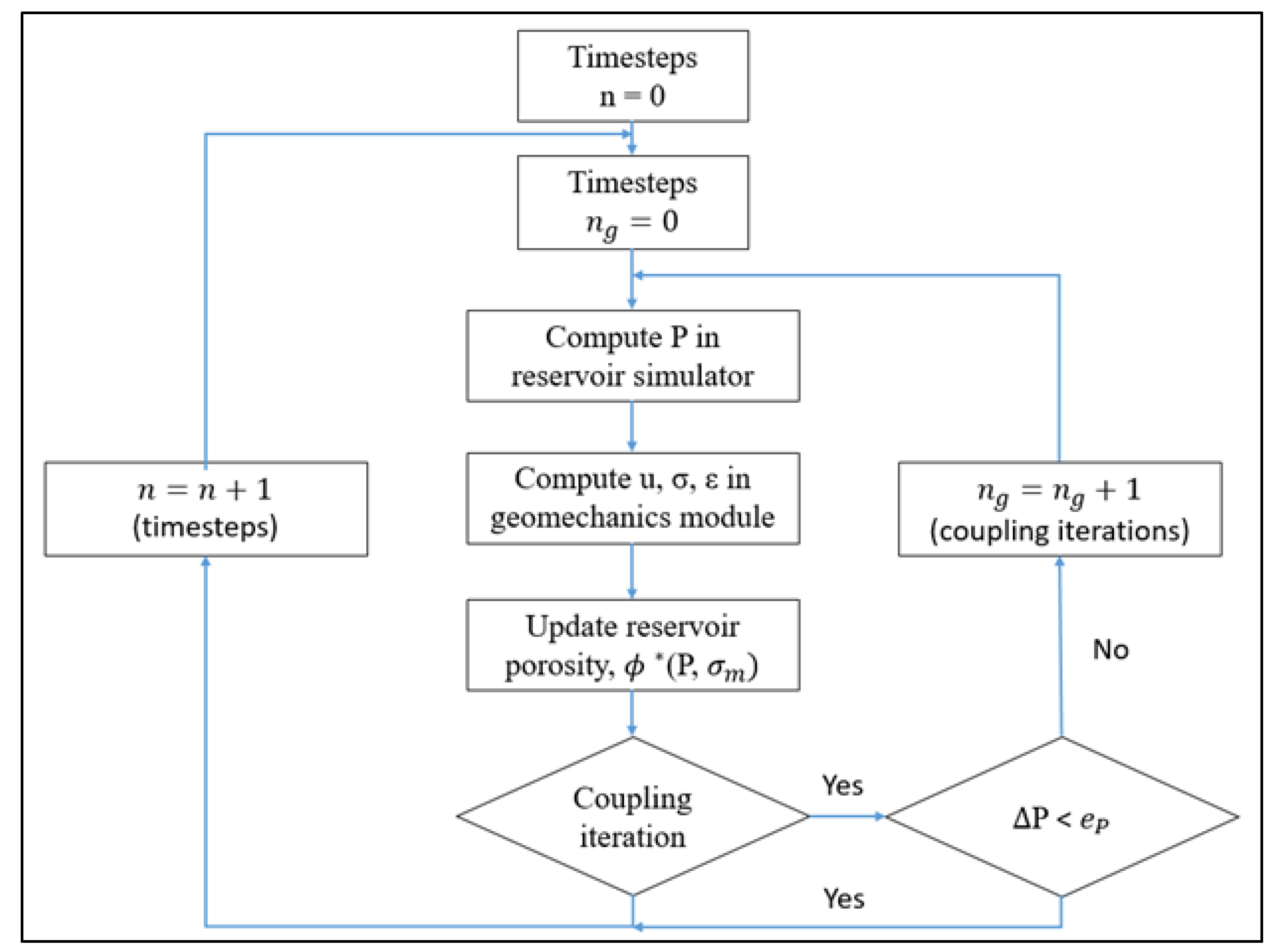
The process involves integrating geomechanical features with a dual permeability model for ultralow permeability formations using a compositional simulator commonly used by the oil and gas industry. The methodology is designed to simulate the growth of fractures during hydraulic fracturing and to optimize the injection process to maximize oil recovery. The dual permeability model for naturally fractured formations is integrated with the geomechanical features of reservoir rocks to simulate hydraulic fracture geometries. The model employs the following two sets of fundamental equations: one for the fluid flow within porous medium and another for the deformation of the rock. The fluid-flow equations encompass the principles of mass conservation and Darcy’s law, while the equations for rock deformation comprise the concepts of deformation, strain, and stress.
The iterative coupled approach is employed to solve the fluid flow and rock deformation equations. This approach is chosen for its reliability and efficiency [9]. The steps involved in the iterative coupling technique are (1) Initial pressure is calculated using the reservoir flow simulator at a specified timestep; (2) Pressure is transmitted to the geomechanics simulator to calculate displacement, strain, and stress; (3) reservoir porosity, influenced by pressure and stress, is updated using volumetric strain. The updated porosity is used to recompute reservoir pressure. (4) the recalculated pressure is sent back to the geomechanics simulator for updated deformation calculations. The process iterates until a predetermined tolerance is achieved [3,10]. The iterative coupling approach is depicted in Error! Reference source not found., providing a concise summary of its diagram.
2.1.1. Modeling of Hydraulic Fracture’s Permeability
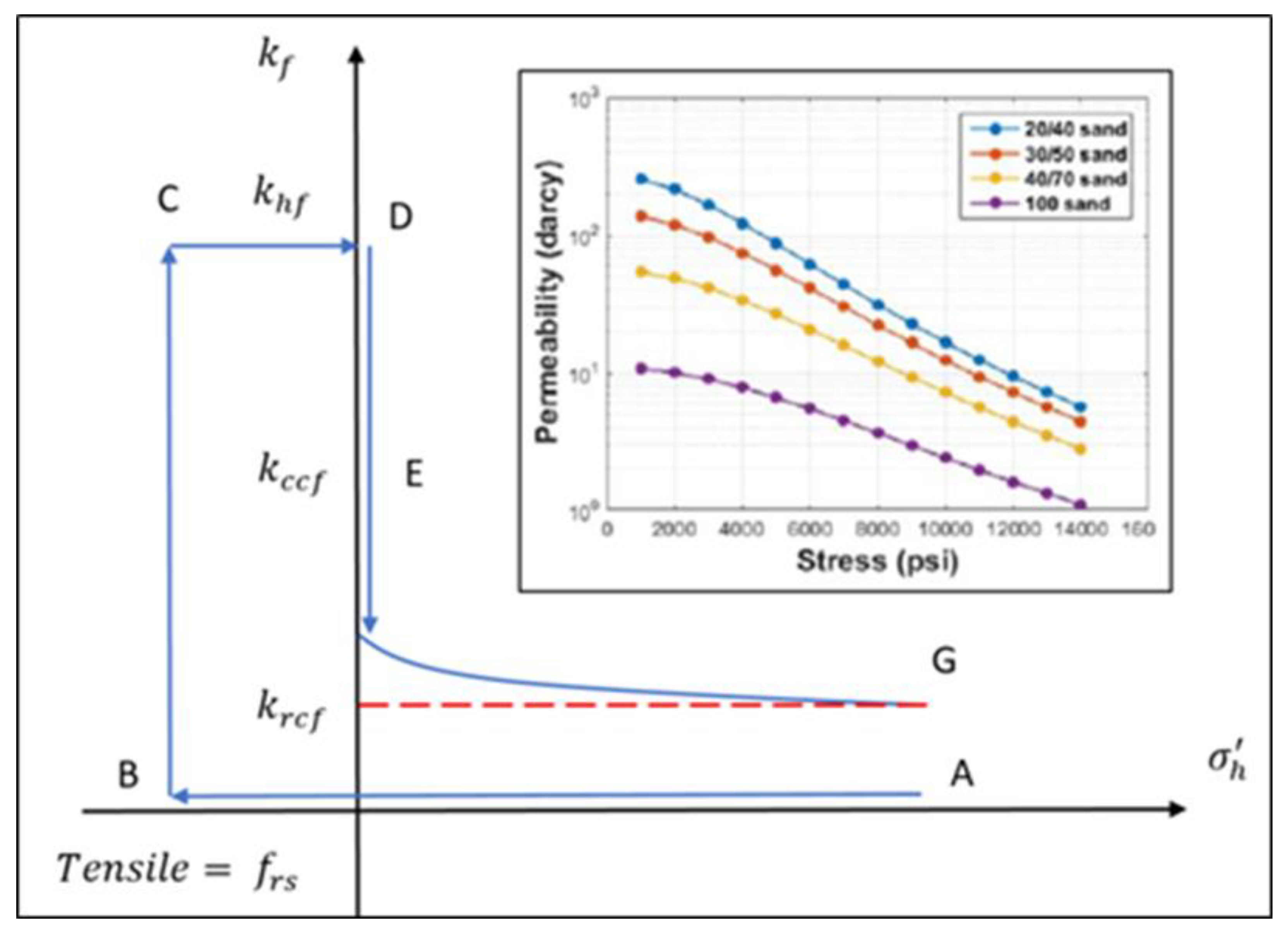
The modified Barton-Bandis model (1983) [13] is used to determine fracture permeability based on closure stress. The hydraulic fracturing process is described (Error! Reference source not found.) as follows:
Fracture Initiation: Initial equilibrium state at point A with effective minimum horizontal stress (σh’). Elevated injection rate and pressure increase pore pressure, reducing σh’ from point A to point B. Fracture initiation at point B when σh’ drops to tensile strength (frs). The fracture permeability (khf) in the stimulated zone is at the maximum value and equal to the intrinsic permeability of the proppant.
Fracture Closure: As stress increases from point C to point D, permeability decreases from khf to closure permeability (kccf). Closure stress acting on fractures supported by proppant gradually reduces fracture permeability to residual fracture permeability (krcf).
2.1.2. CO2 Huff-n-Puff development
After primary recovery, a field-scale development to evaluate different injection scenarios and optimize CO2 huff-n-puff in two depleted fractured horizontal wells. The following four steps generated a detailed optimization workflow for CO2 enhanced oil recovery (CO2-EOR) application in the field
Fluid Model Generation:
The dynamic reservoir simulation modeling begins with generating an equation of state (EOS) fluid model. The compositional reservoir fluid model was fine-tuned to an equation of state using the 3-parameter Peng Robinson model. The laboratory test and analysis performed on the reservoir fluid yielded several components, with the plus fraction beginning from C30. The fluid components were lumped into the seven components to reduce the computational overload. The fluid viscosity was modeled using the Jossi-Stiel-Thodos (JST) correlation. PVT tuning was performed by identifying sensitive fluid properties and regressing them to obtain acceptable matches with the laboratory data. Among the parameters, the critical temperatures, critical pressures, and molecular weights of the fluid components heavily impacted the regression.
Slim Tube Simulation Test:
After the PVT tuning, a 1D slim tube simulation test was performed to estimate the minimum miscibility pressure (MMP). Generally, purchased and recycled CO2 contain impurities that are likely to impact the MMP. Impurities were introduced to the fluid in increments to model real-life impact on CO2-EOR performance.
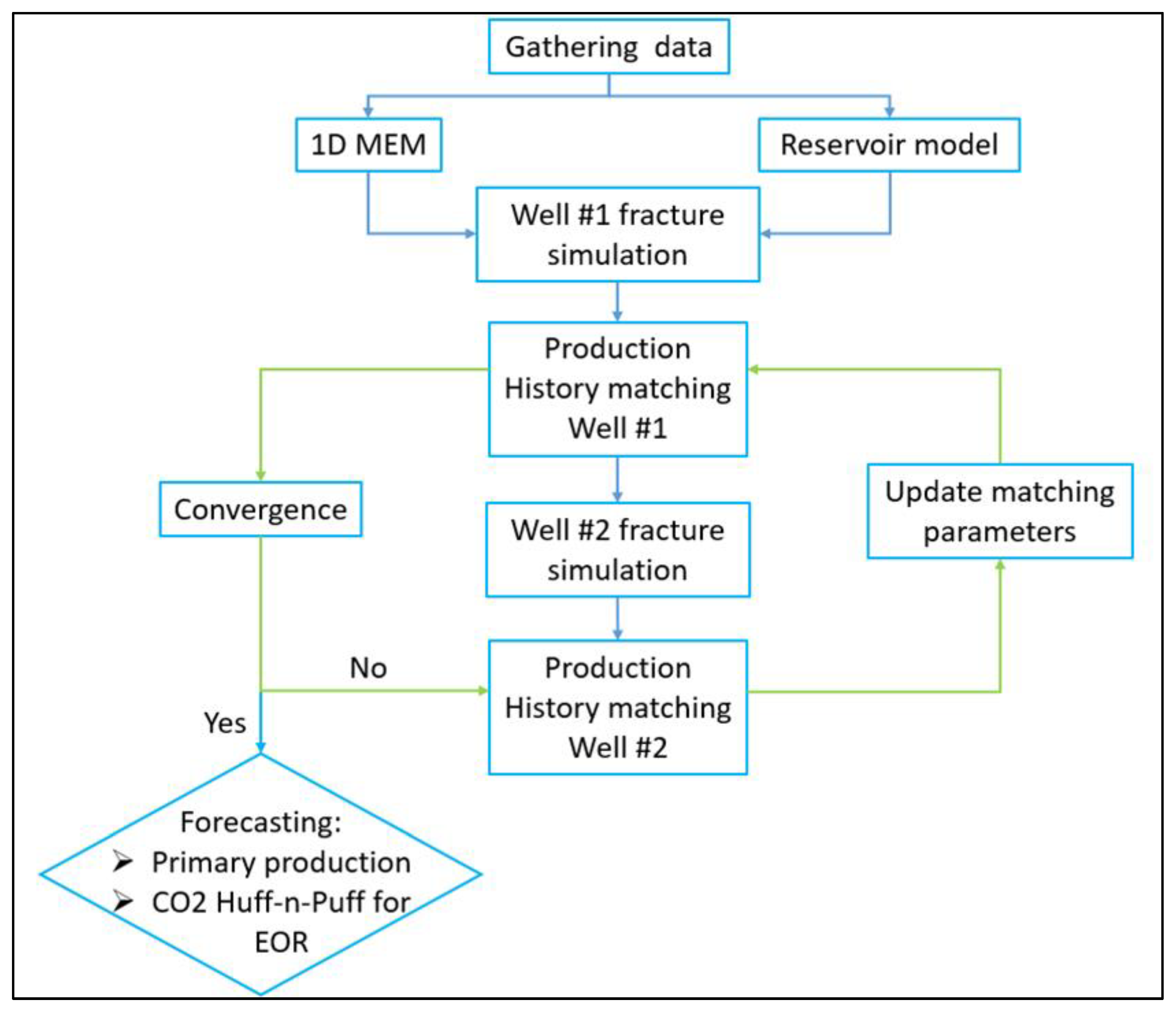
History Matching:
After hydraulic fracturing, the two investigated wells have been producing for about five years and are still active. To verify the quality of the fracture model, several techniques can be deployed, including but not limited to monitoring techniques, post-fractured production analysis, treatment pressure matching for injection periods, and production and flowing bottom hole pressure (BHP) matching for the production phase. In this study, the two wells’ production and flowing bottom hole pressure are available, so they were used as the primary references for validation. Among the above uncertain parameters, reservoir properties, matrix relative permeability curves, and operating conditions are either calculated from log data and calibrated using published data or obtained from well historical data. Since there are two horizontal hydraulic fracture wells modeled, the history matching process in this research is iterative, as demonstrated in Error! Reference source not found. as follows:
Figure 3.
Iterative history matching process for fracture model’s validation.
Field development evaluation:
A comprehensive simulation analysis was conducted to optimize the CO2 huff-n-puff process for CO2-EOR. The study investigated various CO2 injection rates along with different injecting, soaking, and producing time ratios. Several combinations of cycle times were analyzed to determine the optimal cycle. Based on the simulation results, the optimal operating conditions for CO2-EOR in the unconventional Wolfcamp A formation in the Delaware Basin were identified.
Combining a dual permeability model and geomechanical module in a compositional simulation provided a robust framework for optimizing CO2 huff-n-puff injection in depleted horizontal fractured wells.
2.2. Geological Description and Properties
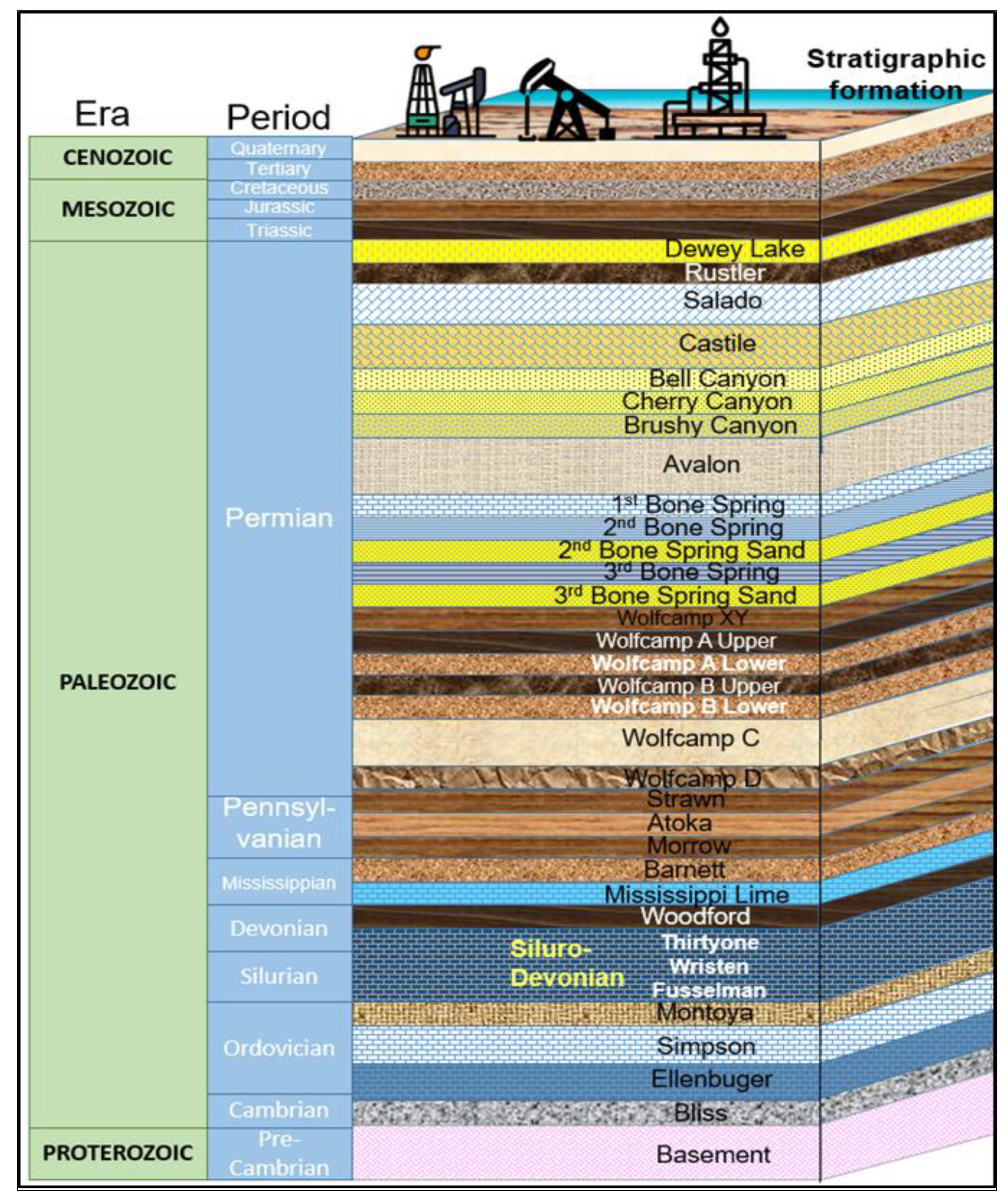
The Wolfcamp formation, which was formed from the late Pennsylvanian to the end Wolfcampian period, extends over all of the Permian Basin. The Wolfcamp formation is an intricate geological unit mostly composed of shale with high organic content and intervals of carbonate rocks that include clay minerals [15]. The sub-basins, including Delaware Basin, Midland Basin, Central Basin Platform, and Delaware, exhibit substantial variations in depth, thickness, and lithology of the Wolfcamp deposition. The heterogeneity of this formation is governed by depositional and diagenetic mechanisms. From a stratigraphic perspective, the Wolfcamp formation consists of four stratified intervals, labeled as the A, B, C, and D sequences, as shown in Error! Reference source not found..
Figure 4.
Schematic stratigraphy of Wolfcamp formation [16].
Figure 4.
Schematic stratigraphy of Wolfcamp formation [16].
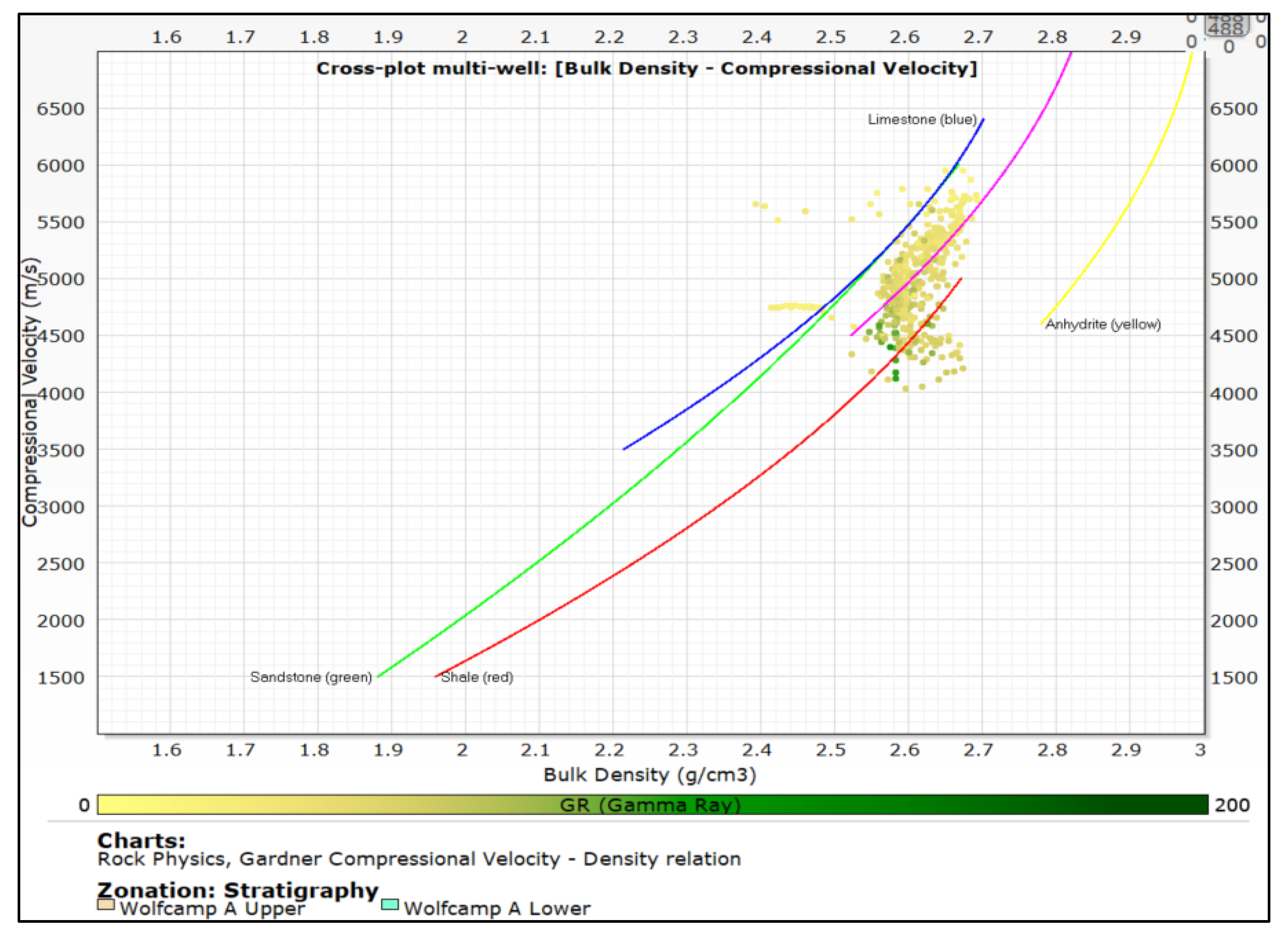
The majority of the present drilling operations in the Delaware and Midland Basins are focused on the Upper Wolfcamp, named as A and B formations. These layers are characterized by a higher abundance of natural gas and more mature phases of hydrocarbon yield compared to the Lower Wolfcamp C and D reservoirs [17]. On top of that, the Wolfcamp A formation consists of alternating layers of shale, siltstone, sandstone, and carbonate rocks (Error! Reference source not found.). The thin interbeds of sandstones and limestones within the shales can act as storage units for hydrocarbons. However, the tight nature of these rocks makes it difficult to conventionally extract oil and gas from them.
Figure 5.
Lithological characteristic of the Wolfcamp A formation.
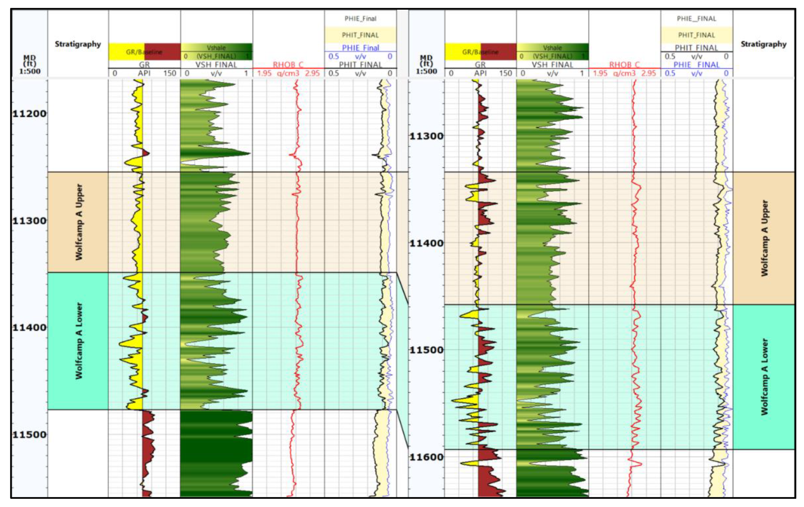
In a recent paper, the authors Bui et al. [18] constructed a detailed methodology and equations to estimate the petrophysical parameters and develop a 1D mechanical earth model for the Third Bonespring Sand in the Delaware basin. This study continues to use the same approach and formulas to calculate essential petrophysical elements for the Wolfcamp A formation at Lea County, such as shale volume, total and effective porosities. The findings show that the average shale volume is about 55%, the average total porosity is 0.09, and the effective porosity is 0.05 (Error! Reference source not found.).
Figure 6.
Petrophysical interpretation of Wolfcamp A formation in the offset wells.
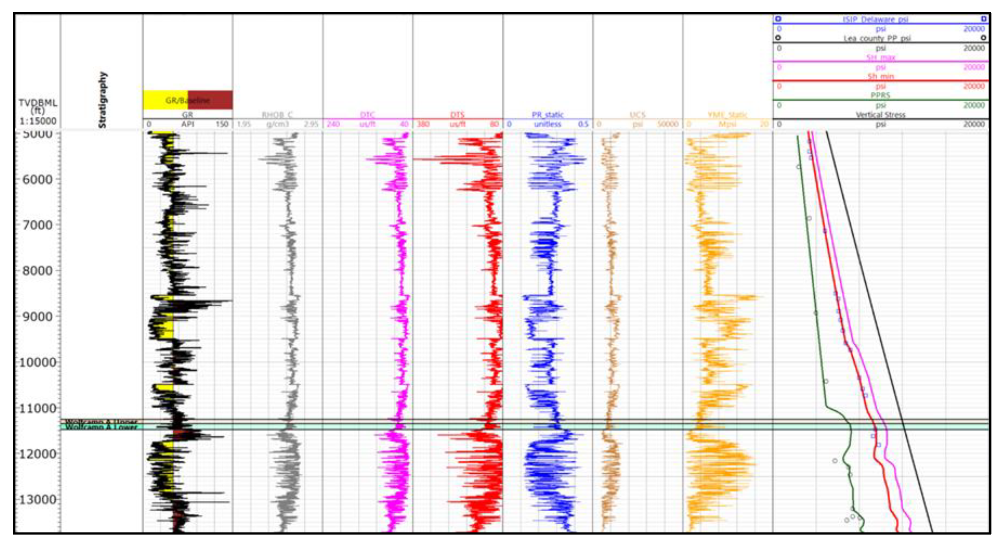
From the perspective of the in-situ stresses, the developed 1D geomechanical model illustrates that the pore pressure gradient increases from 0.6 psi/ft at the top of the Wolfcamp A formation to a peak of 0.7 psi/ft. The minimum and maximum horizontal stresses are characterized by pressure gradient of 0.79 psi/ft and 0.87 psi/ft respectively. In addition, the vertical stress indicates a pressure gradient of 1.1 psi/ft (Error! Reference source not found.).
Figure 7.
1D geomechanical model for the Wolfcamp A formation.
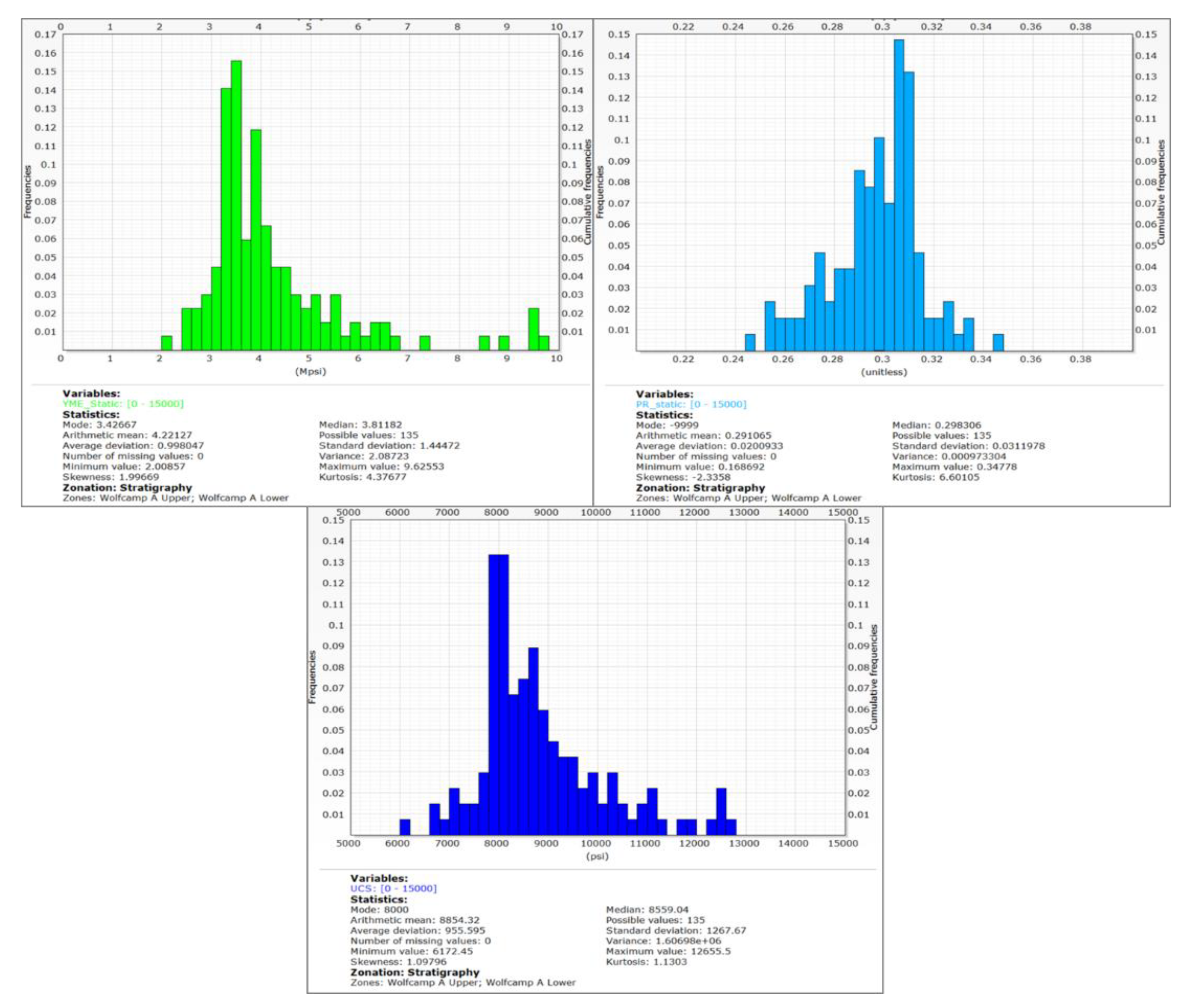
The rock properties and strengths are essential in representing the mechanical behavior of the reservoir [19,20,21] and are critical for hydraulic fracturing simulation. The statistical data pertaining to the Wolfcamp A formation in Error! Reference source not found. displays average values of 4.2 Mpsi for static Young’s modulus, 0.29 for static Poisson ratio and 8854 psi for unconfined compressive strength (UCS).
Figure 8.
Statistics of rock properties and strength in the Wolfcamp A formation.
2.3. Simulation Setup
The numerical model employed for this study was a dual-permeability model, which was developed using the Computer Modelling Group (CMG) - GEM reservoir simulator. This widely accepted simulator allows for the detailed representation and simulation of fluid flow and other geomechanics-hydrodynamic behaviors. The entire reservoir is discretized into 103 x 101 x 6 grid blocks in the x, y, and z directions, with total length in x- and y-direction 5,150 ft and 2,500 ft, respectively. The total length of the reservoir in the x-direction is 5,150 feet, while the size in the y-direction is 2,500 feet. The vertical extent of the reservoir, from top to bottom, ranges from 11,300 feet to 11,500 feet below the surface, giving an average formation thickness of 250 feet. This detailed grid setup deployed formation tops and well logs of four nearby vertical wells in the Wolfcamp A formation, allowing a precise simulation of the field operations. A summary of the critical reservoir properties is provided in Error! Reference source not found., which includes data on porosity, permeability, and other relevant petrophysical and geomechanical parameters.

Table 1.
Summary of reservoir properties.
| Properties | Values |
|---|---|
| Top formation true vertical depth, TVD | 11,300 ft |
| Average reservoir permeability, k | 3.5e-4 mD |
| Average effective matrix porosity, ϕ | 0.04 |
| Reservoir temperature, T | 169 F |
| Initial pore pressure, P | 6887 psi |
| Initial water saturation, Swi | 0.6 |
| Critical oil saturation, Soc | 0.2 |
| Oil API | 43.5 |
| Gas gravity | 0.483 |
| Young’s modulus of matrix rock, E | 4.22e6 psi |
| Poisson’s ratio of matrix rock, v | 0.297 |
| Overburden stress gradient | 1.09 psi/ft |
| Minimum horizontal stress gradient | 0.7 psi/ft |
| Maximum horizontal stress gradient | 0.86 psi/ft |
2.4. Simulation of CO2 Injection
Cyclic CO2 injection was initiated using the GEM compositional simulator for both wells after five years of primary depleted production. This process aimed to enhance oil recovery by utilizing CO2 to displace the remaining hydrocarbons in the reservoir, thereby increasing production efficiency and prolonging the reservoir’s productive life.
During the injection phase, CO2 was injected into the reservoir at a constant rate of one million standard cubic feet (MMscf) per day over 30 days. This phase aimed to refill the reservoir’s void created by the prior production phase, effectively repressurizing the reservoir above the MMP. The injection was carefully controlled to maintain a BHP limit of 7,000 psi to ensure the formation integrity and prevent potential CO2 leakage. Over the first injection phase, a volume of 30,000 thousand cubic feet (Mcf) of CO2 was injected into the reservoir. Following the injection phase, a soaking period of 30 days was implemented. During this soaking time, the injected CO2 was allowed to diffuse and interact with the reservoir fluids, thus swelling the residual oil and decreasing its viscosity. The soak period is critical as it will enable the CO2 to effectively mobilize the trapped hydrocarbons. After the soaking period, the reservoir was put back into production for 150 days. This production phase allowed the mobilized hydrocarbons to be produced to the surface, taking advantage of the increased reservoir pressure and improved fluid flow dynamics resulting from the CO2 injection and soak period.
To verify the efficiency of the CO2 huff-n-puff process, a total of 28 cycles of CO2 injection, soaking, and production were implemented. Each cycle involved injecting CO2 at the specified rate, allowing a soak period, and producing for the designated time. This repetitive process helped to maximize hydrocarbon recovery and provided valuable data on the performance and effectiveness of cyclic CO2 injection in enhancing oil recovery.
3. Results
3.1. Simulation of Fracture Geometry
The Well #1 and Well #2 were fractured with 23 and 24 stages, respectively, with the same injection rate, proppant type, and amount of fracture fluid. According to fracture reports, the fracture treatment of the two wells is summarized in Error! Reference source not found.. Each stage of the investigated wells is fractured with slick water using 100 mesh and 40/70-mesh sand and 85 barrels per minute (bpm) fluid rate in 103 minutes.
Table 2.
Fracture treatment from the field.
| Average Pump Rate per Fracture Stage, bpm | Average Pump Time per Stage, min | Proppant Type | |
|---|---|---|---|
| Well #1 | 85 | 103 | 100 mesh; local 40/70 Sand |
| Well #2 | 85 | 103 | 100 mesh; local 40/70 Sand |
When the tensile failure criterion is met, fractures initiate and simultaneously increase the minimum horizontal stress in the adjacent zone, as illustrated in Error! Reference source not found.. Previous research [1,8,14,22,23,24] describes this phenomenon using the concept of stress shadowing. This additional stress due to stress shadowing increases the effective minimum horizontal stress, which in turn reduces the likelihood of opening the formation in the desired direction. The direction of fracture propagation may vary depending on the orientation of the existing minimum horizontal stress and the magnitude of the added stress.
Figure 9.
Illustration of stress shadowing effects.
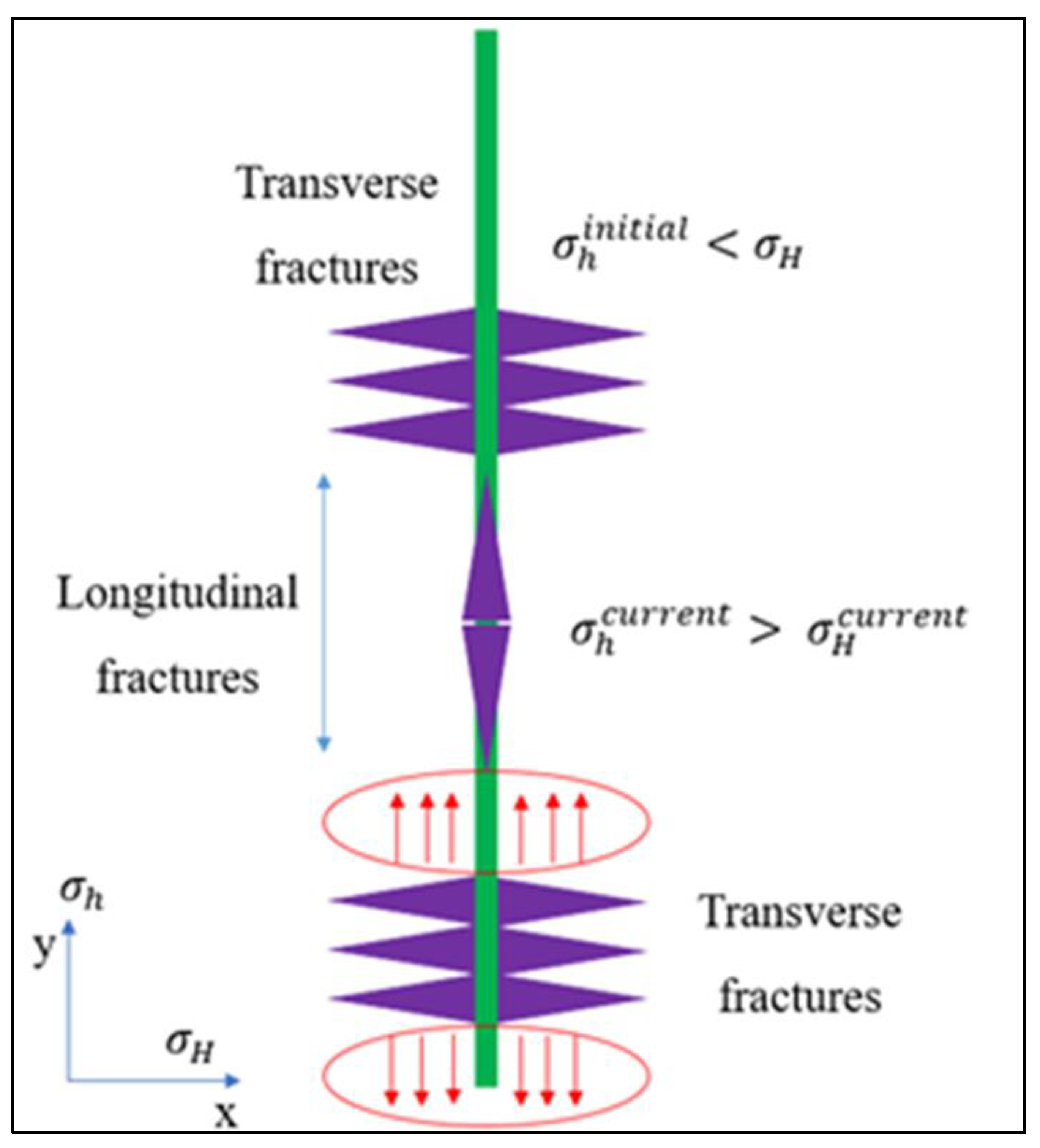
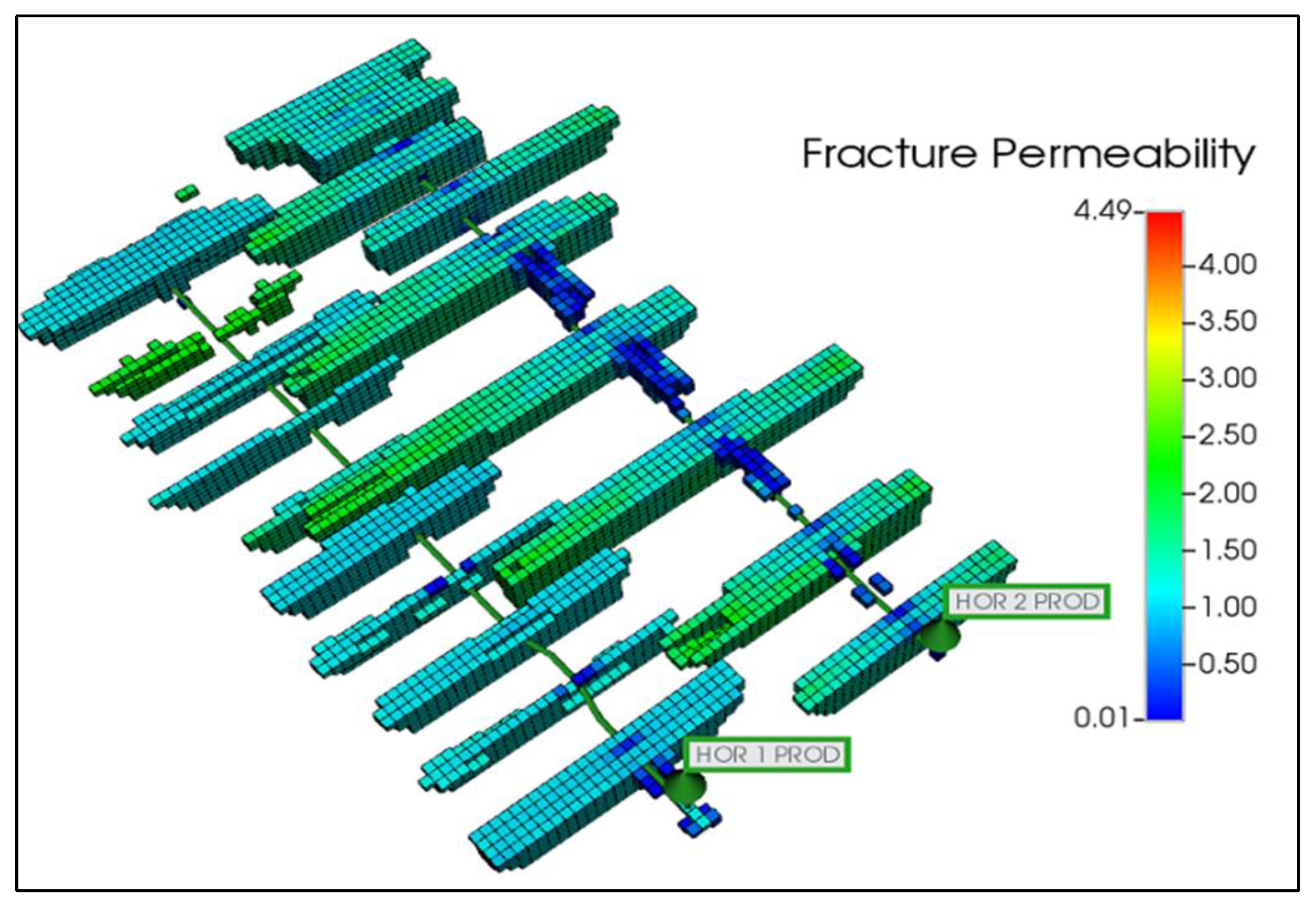
As a result, fractures in such scenarios do not grow symmetrically. Instead, they propagate both transversely and longitudinally, favoring zones of lower effective stress. The fracture simulation results exhibit both symmetric and asymmetric fracture geometries, with fracture lengths ranging from 400 to 1,250 feet and fracture heights spanning the entire formation thickness, as shown in Error! Reference source not found..
Figure 10.
Fracture geometry of Well #1 and Well #2.
3.2. Production History Matching
After hydraulic fracturing, Well #1 had been producing for one year before Well #2 was fractured. To verify the quality of the fracture model, several techniques can be deployed. In this study, the production and flowing BHP of the two wells were used as primary references for validation.
For production history matching, various parameters can be adjusted, including reservoir properties, relative permeability curves, and operating parameters. In unconventional reservoirs, where induced hydraulic fractures are commonly used, post-fractured permeability (or residual fracture permeability) and the relative permeability curves of the fracture system are the most sensitive parameters affecting reservoir fluid flow. To achieve a reasonable matching result, it is crucial to reduce the number of uncertainties considered. Typically, uncertain parameters such as reservoir properties, matrix relative permeability curves, and operating conditions are calculated from log data, calibrated using published data, or obtained from historical well data. This makes fracture permeability and the relative permeability curves in the fracture system particularly sensitive, as there is limited information available from the literature and laboratory measurements. Consequently, closure fracture permeability, residual fracture permeability, and relative permeability curves in the fracture system were treated as the primary varying parameters to achieve production and flowing bottom hole pressure (BHP) matching.
Ojha et al. (2017) [25] measured various shale samples to obtain the average relative permeability curves for the Wolfcamp formation. The relative permeability curves of water-oil and gas-liquid systems from Ojha et al. (2017) [25] were integrated into the base model to simulate multiphase flow. Error! Reference source not found. lists the parameters considered for matching the production data.

, Error! Reference source not found., Error! Reference source not found. show the history-matching results for the fluids produced from individual wells. Error! Reference source not found. presents the history-matching results for the oil rate and cumulative production of the entire field. The matching results indicate that the quality of the fracture model is sufficient to represent the reservoir accurately for further analyses and forecasting.
Table 3.
Final history matching parameters.
| Matching Parameters | Base Values | Final Values |
|---|---|---|
| Closure Fracture Permeability, mD | 6 | 4.8 |
| Residual Fracture Permeability, mD | 3 | 2.4 |
| Fracture Relative Permeability Curves | ||
| Gas relative permeability at connate liquid | 0.95 | 0.9 |
| Oil relative permeability at connate water | 0.6 | 0.7 |
| Oil relative permeability at connate gas | 0.6 | 0.7 |
| Water relative permeability at irreducible oil | 0.9 | 0.85 |
| Curvature exponent of water curve in water-oil system | 2 | 1.5 |
| Curvature exponent of oil curve in water-oil system | 2 | 2 |
| Curvature exponent of gas curve in gas-liquid system | 2.4 | 2.2 |
| Curvature exponent of oil curve in gas-liquid system | 2 | 2 |
| Irreducible water saturation | 0.4 | 0.4 |
| Residual oil saturation in oil-water system | 0.2 | 0.15 |
| Residual (critical) gas saturation | 0.05 | 0.05 |
Figure 11.
(a) History matching oil rate Well #1; (b) History matching oil rate Well #2.
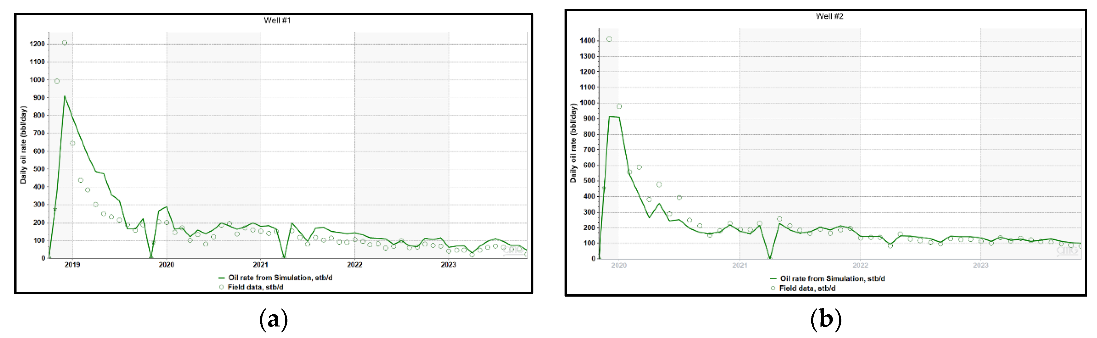
Figure 12.
(a) History matching gas rate Well #1; (b) History matching gas rate Well #2.
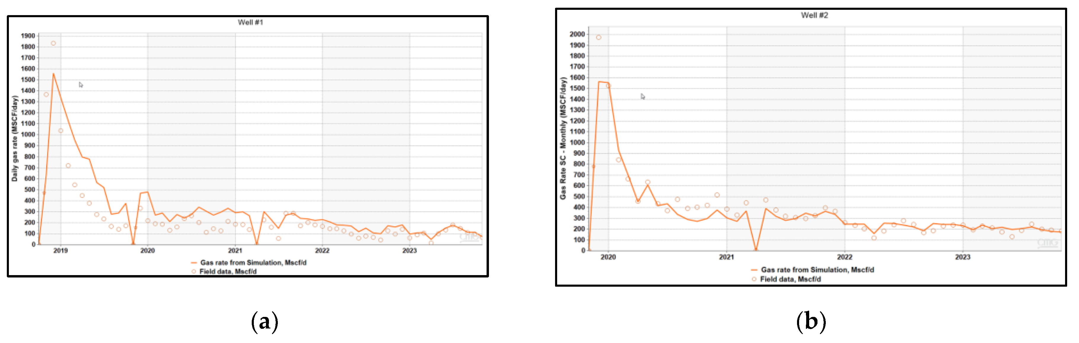
Figure 13.
(a) History matching water rate Well #1; (b) History matching water rate Well #2.
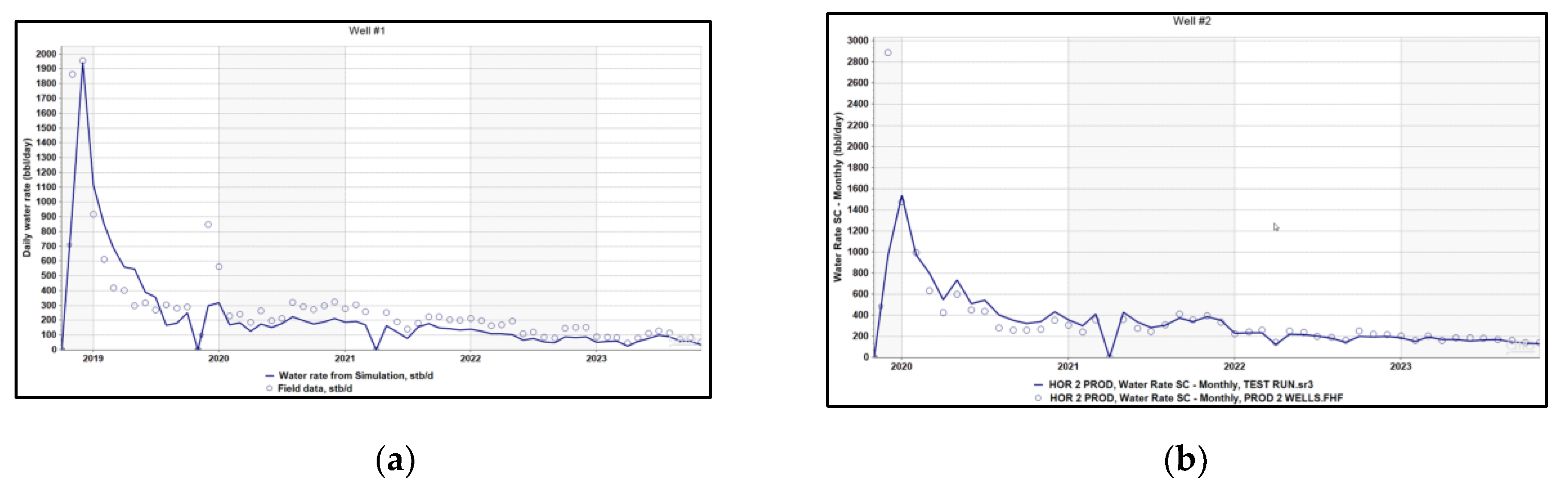
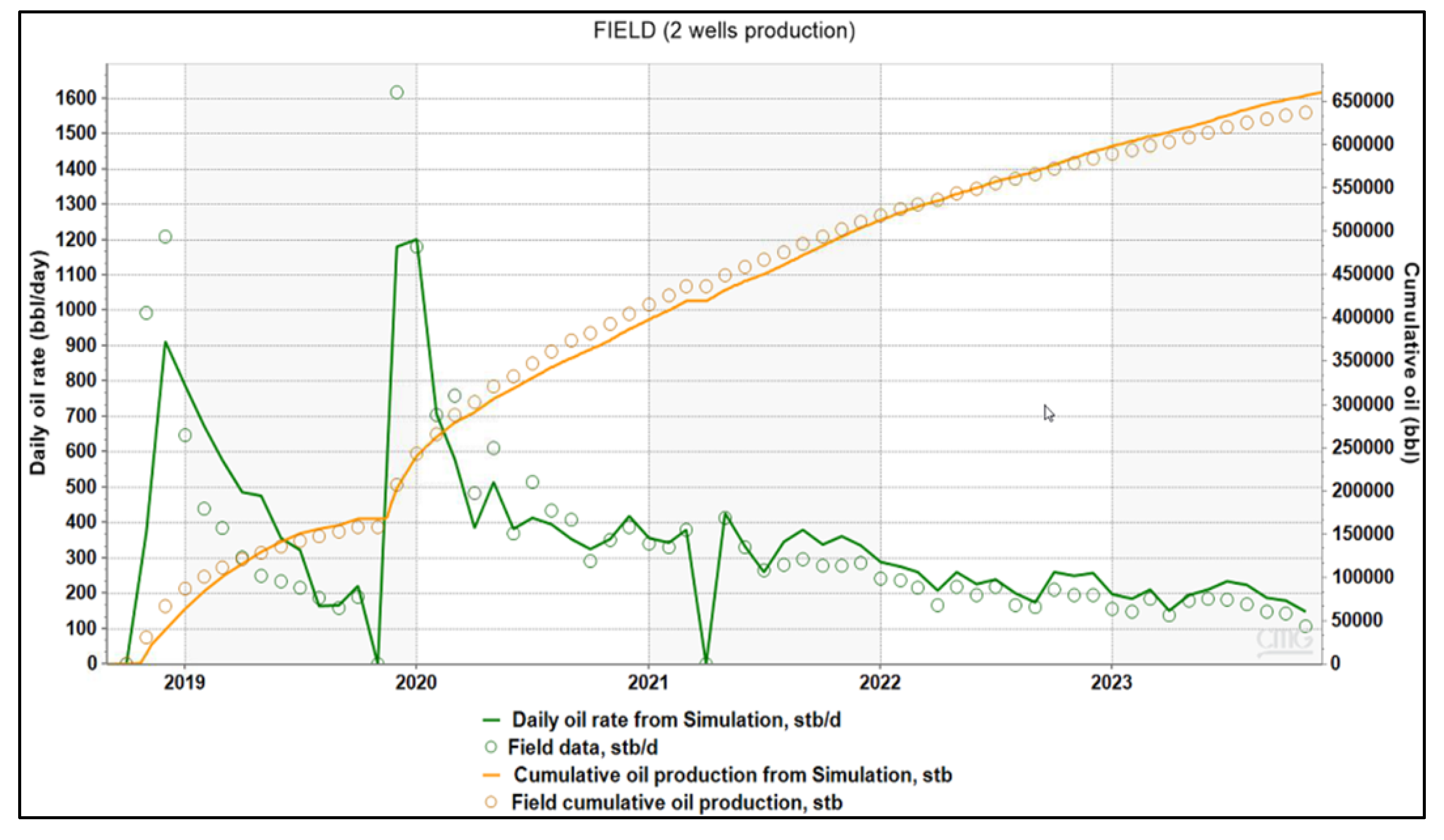
Figure 14.
History matching oil cumulative and oil rate of entire field.
3.3. Estimating Minimum Miscibility Pressure for CO2 and the Reservoir’s Oil
3.3.1. Oil Composition
The oil composition data (Error! Reference source not found.) and the component properties (Error! Reference source not found.) of PVT for the Wolfcamp A formation are provided below. The composition presented in Error! Reference source not found. was based on the Bonespring formation laid right above the Wolfcamp A formation [11]. The C7+ fraction has been de-lumped into four pseudo-components to ensure a more accurate PVT model. In this study, PVT calculation and properties interactions among various compositions were performed through an equation-of-state simulator to feed the hydrodynamic modeling performed by numerical simulation. This is the preferred method for the determination of MMP, where the laboratory-measured phase behavior data is available for fine-tuning an equation of state.
Table 4.
Fluid composition fraction.
| Component | Mole Percent (%) |
|---|---|
| N2 | 1.07 |
| CO2 | 0.11 |
| CH4 | 46.98 |
| C2H6 | 10.66 |
| C3H8 | 6.92 |
| IC4 | 3.22 |
| NC4 | 1.18 |
| IC5 | 1.54 |
| NC5 | 1.21 |
| FC6 | 1.82 |
| HYP01 | 7.69 |
| HYP02 | 10.45 |
| HYP03 | 5.79 |
| HYP04 | 1.36 |
Table 5.
Key properties of fluid components.
| No. | Component | Pc (atm) | Tc (K) | Acentric Factor | MW | SG |
|---|---|---|---|---|---|---|
| 1 | N2 | 33.50 | 126.20 | 0.04 | 28.01 | 0.81 |
| 2 | CO2 | 72.80 | 304.20 | 0.23 | 44.01 | 0.82 |
| 3 | CH4 | 45.40 | 190.60 | 0.01 | 16.04 | 0.30 |
| 4 | C2H6 | 48.20 | 305.40 | 0.10 | 30.07 | 0.36 |
| 5 | C3H8 | 41.90 | 369.80 | 0.15 | 44.10 | 0.51 |
| 6 | IC4 | 36.00 | 408.10 | 0.18 | 58.12 | 0.56 |
| 7 | NC4 | 37.50 | 425.20 | 0.19 | 58.12 | 0.58 |
| 8 | IC5 | 33.40 | 460.40 | 0.23 | 72.15 | 0.63 |
| 9 | NC5 | 33.30 | 469.60 | 0.25 | 72.15 | 0.63 |
| 10 | FC6 | 32.46 | 507.50 | 0.28 | 86.00 | 0.69 |
| 11 | HYP01 | 30.79 | 570.66 | 0.28 | 102.13 | 0.76 |
| 12 | HYP02 | 21.84 | 670.57 | 0.46 | 157.05 | 0.81 |
| 13 | HYP03 | 14.12 | 802.17 | 0.76 | 264.75 | 0.87 |
| 14 | HYP04 | 9.45 | 943.83 | 1.14 | 452.25 | 0.93 |
3.3.2. MMP Determination
In CO2-EOR design, the MMP is a crucial parameter for improving oil recovery from the porous medium and achieving maximum displacement efficiency. MMP is defined as the lowest pressure at which the injected gas becomes dynamically miscible with the reservoir oil. Although MMP can be accurately measured using laboratory experimental methods, these methods are often costly and time-consuming [26]. Therefore, in this research, the slim tube test was simulated using a one-dimensional compositional reservoir model.
To estimate the MMP between the injected CO2 and the oil composition for the study area - the Wolfcamp A reservoir - a comprehensive suite of slim tube simulations was conducted using the CMG-GEM software. These simulations are essential for determining the pressure at which CO2 can effectively mix with the reservoir oil without forming two separate phases. By conducting these slim tube simulations, which mimic the reservoir conditions and fluid interactions, it was able to accurately establish an MMP of approximately 4300 psi (Error! Reference source not found.). This value is critical for designing and optimizing enhanced oil recovery (EOR) processes, as it ensures that the injected CO2 will efficiently mix with the reservoir oil, thereby improving recovery rates and maximizing production from the investigated formation.
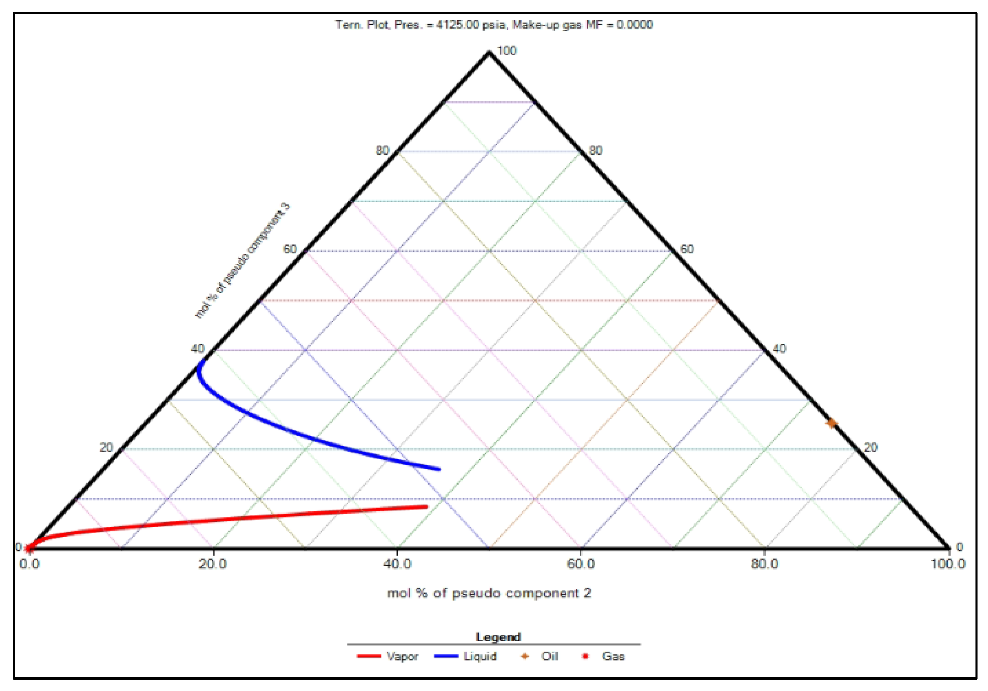
Also, a cell-to-cell simulation was conducted using the aforementioned PVT fluid model with pure CO2 injection to compare with 1D slim-tube simulation and to better understand the miscibility behavior between the CO2 and reservoir oil. This simulation was performed using the CMG-Winprop simulator, allowing for a detailed examination of how CO2 interacts with the oil at different pressures and temperatures. The results from this simulation indicated that the MMP is approximately 4125 psi (Error! Reference source not found.). Accurately estimating the MMP for the Wolfcamp A shale formation is crucial for optimizing CO2 injection strategies and ensuring the successful implementation of the CO2 huff-n-puff technique in unconventional formations.
Figure 15.
Slim-tube simulation result for MMP.
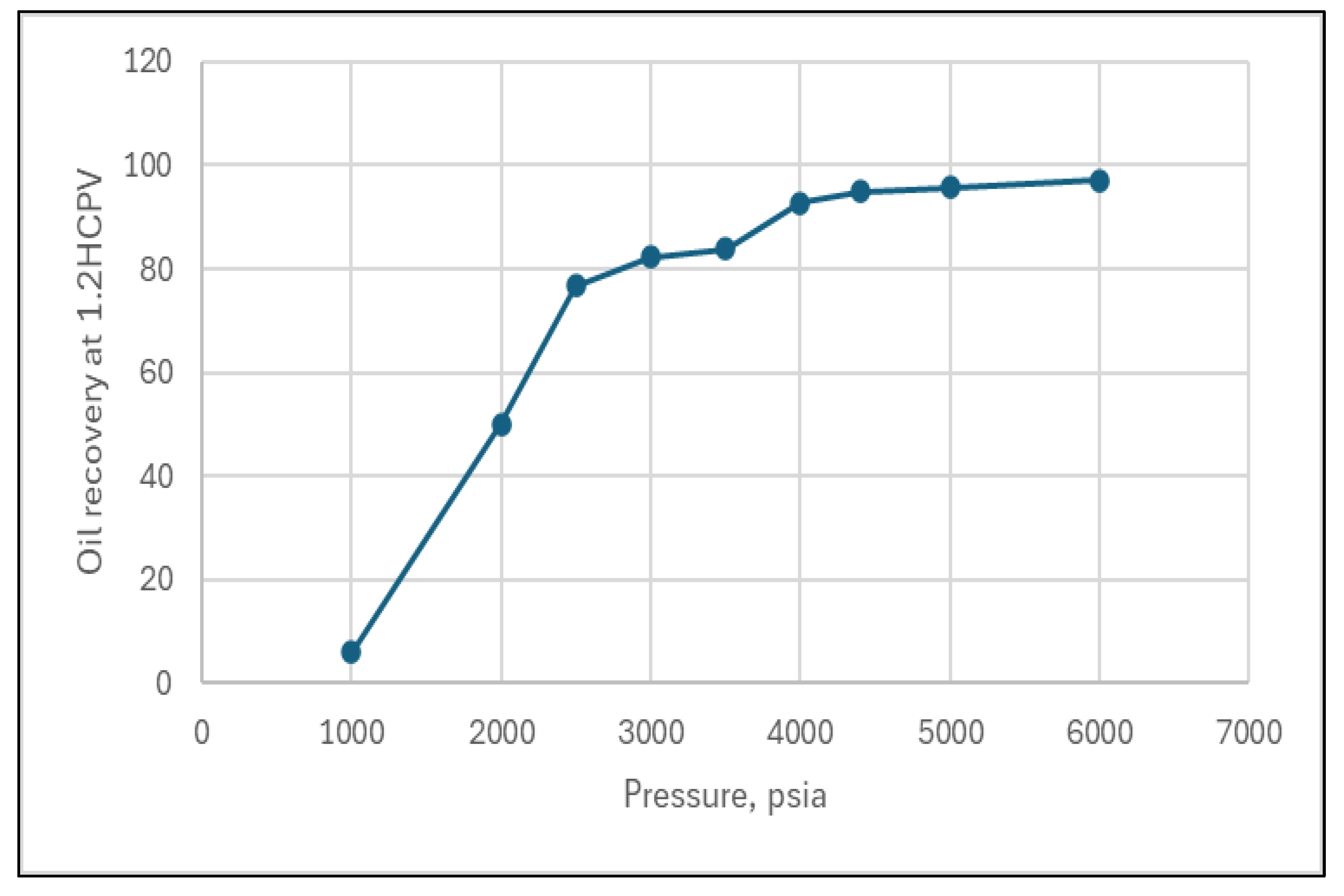
Figure 16.
Cell-to-cell simulation result for MMP.
3.4. Modeling of Cyclic CO2 Injection
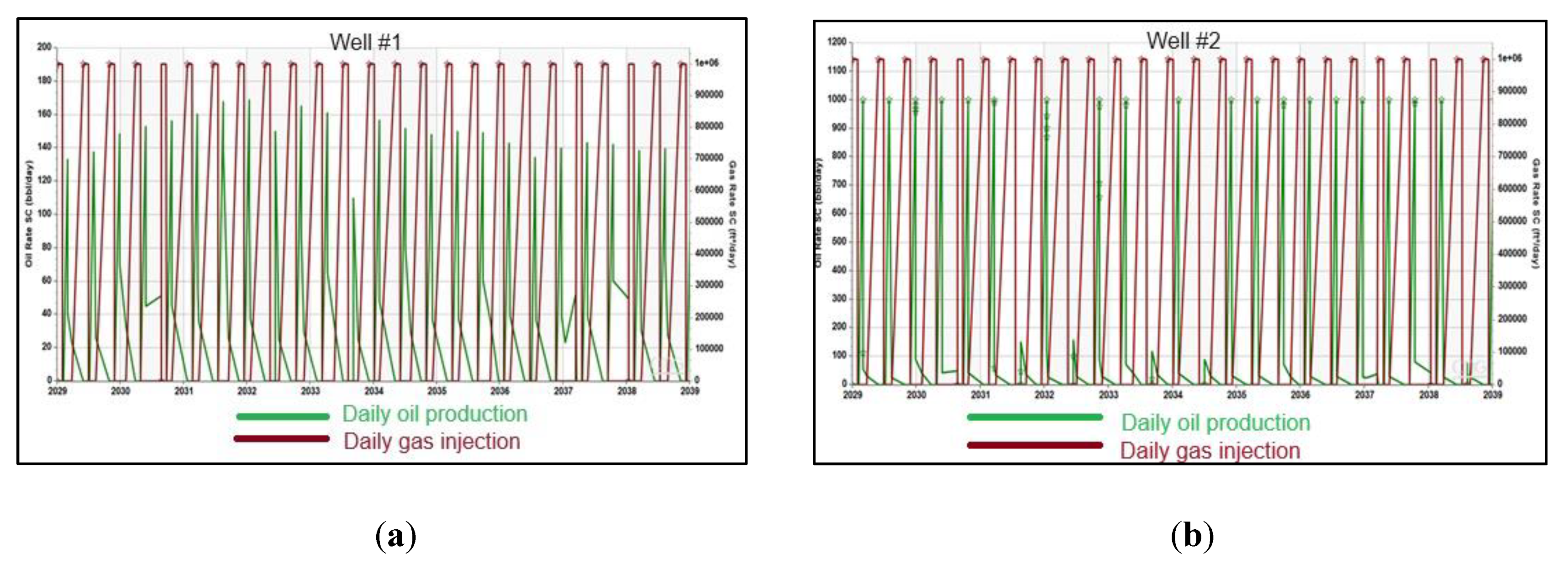
Error! Reference source not found. illustrates the detailed oil and gas production rate for 28 consecutive cycles, covering a producing period of 10 years. These cycles involve a repetitive process of cyclic CO2 injection, soaking, and production. The data is shown for both studying wells, with the CO2 being injected at a consistent rate of 1 million standard cubic feet per day per well (MMscf/d/well). The figure provides a comprehensive view of how the hydrocarbon production rates fluctuate and evolve over time with the implementation of this CO2 huff-n-puff.
Figure 17.
(a) Oil and gas injection rate of Well #1 associated with 1 MMscf/d CO2 injection; (b) Oil and gas injection rate of Well #2 associated with 1 MMscf/d CO2 injection.
Figure 17.
(a) Oil and gas injection rate of Well #1 associated with 1 MMscf/d CO2 injection; (b) Oil and gas injection rate of Well #2 associated with 1 MMscf/d CO2 injection.
Error! Reference source not found. compares cumulative oil production between the enhanced case and the base case, in which no CO2 injection was deployed for both wells. Well #1 shows an improvement of 2% in cumulative oil, whereas Well #2 expresses a development of 6% using the CO2 huff-n-puff technique. Specifically, the incremental oil production from Well #2 is approximately 28,000 STB, representing a 6.3% improvement over primary depletion. In contrast, Well #1 exhibits a significantly lower increment of 10,000 STB, corresponding to only a 2% production enhancement. The difference in CO2-EOR percentage between the two wells comes from production starting time and treatment additives in the fracturing fluid. Note that Well #1 started producing one year before the fracturing of Well #2, so the absolute cumulative oil production without CO2 enhancement was higher than that of Well #2, making the percentage of oil increment in Well #1 lower than Well #2. On the other hand, although both wells were hydraulically fractured by slick water, the additive’s concentration differed. Well #2 was treated with a higher concentration of hydrochloric acid, salts, and corrosion inhibitors than Well #1, indicating an improved downhole treatment, which can further aid in the tertiary recovery process using CO2 injection.
Figure 18.
(a) Cumulative oil production of Well #1 associated with 1 MMscf/d CO2 injection; (b) Cumulative oil production of Well #2 associated with 1 MMscf/d CO2 injection.
Figure 18.
(a) Cumulative oil production of Well #1 associated with 1 MMscf/d CO2 injection; (b) Cumulative oil production of Well #2 associated with 1 MMscf/d CO2 injection.
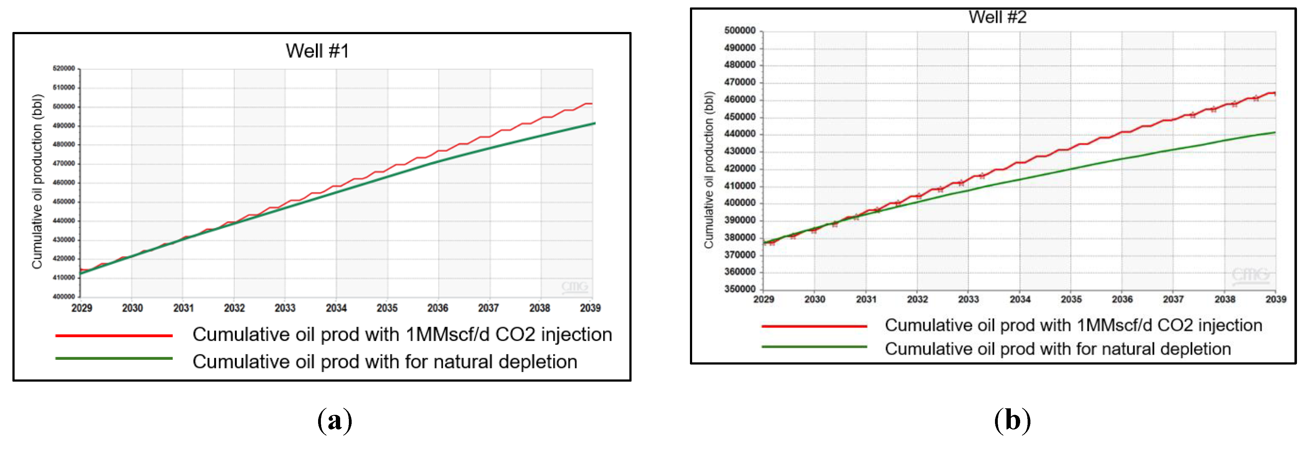
With the difference in downhole treatment between the two wells, the marked disparity in production improvement is hypothesized to be primarily attributable to formation damage in Well #1. However, analyzing formation damage mechanisms on the production performance of Well #1 is out of the scope of this study and will be scrutinized in future work. Given this substantial performance differential between the two wells, subsequent sensitivity analyses will focus exclusively on Well #2 to optimize production parameters and better understand the factors influencing EOR in this reservoir.
3.5. Cyclic Times Sensitivity
For each scenario, a total of 24 cycles of CO2 huff-n-puff were simulated on Well #2. The total time of one cycle is 150 days, with injection, soak, and production periods varying to determine the optimal operating conditions. The cumulative volume of CO2 injection each cycle was 30 MMscf. A summary of various CO2 huff-n-puff strategies is presented in Error! Reference source not found.. The ultimate goal of this sensitivity analysis is to maximize total oil recovery. Error! Reference source not found. summarizes the simulation parameters and results. Compared to the base case with no CO2 injection, the oil recovery improved by 4% to 8%. After running the first seven scenarios, a linear regression model was fitted to the dataset to find the optimal injection-soak time combination.
Table 6.
Summary of different CO2 huff-n-puff strategy.
| Case number | CO2 Injection Rate, MMscf/d | Injection Time, Day | Soaking Time, Day | Production Time, Day |
|---|---|---|---|---|
| Case 1 | 1 | 30 | 30 | 90 |
| Case 2 | 1 | 30 | 20 | 100 |
| Case 3 | 1 | 30 | 50 | 70 |
| Case 4 | 1 | 30 | 10 | 110 |
| Case 5 | 0.5 | 60 | 15 | 75 |
| Case 6 | 2 | 15 | 20 | 115 |
| Case 7 | 2 | 15 | 10 | 125 |
| Case 8 | 2 | 15 | 30 | 105 |
Table 7.
Summary of CO2-EOR process.
| Scenario | Cumulative Oil Production | Cumulative CO2 | Estimated CO2 Storage (mil.lbs) | ||
|---|---|---|---|---|---|
| Total (STB) | Incremental EOR (STB) | Injection (mil.lbs) | Production (mil.lbs) | ||
| Base case(no CO2-EOR) | 441,912 | Not applicable | |||
| Case 1 | 469,891 | 27,979 | 87.51 | 66.52 | 20.99 |
| Case 2 | 467,252 | 25,340 | 87.51 | 71.87 | 15.64 |
| Case 3 | 464,271 | 22,359 | 87.51 | 69.81 | 17.7 |
| Case 4 | 469,820 | 27,908 | 87.51 | 74.68 | 12.84 |
| Case 5 | 459,431 | 17,519 | 87.01 | 76.55 | 10.45 |
| Case 6 | 472,894 | 30,982 | 87.51 | 74.01 | 13.51 |
| Case 7 | 472,773 | 30,861 | 87.51 | 69.56 | 17.95 |
| Case 8 | 464,480 | 22,568 | 87.51 | 68.04 | 19.47 |
Analyzing eight scenarios presented in Table R4, Case 1 stands out as having the highest CO2 storage capacity, surpassing Case 7 by approximately 17% and Case 6 by about 55%. This makes Case 1 the most effective in terms of CO2 sequestration. However, this advantage comes with a trade-off in oil production. Case 1 yields approximately 9.7% less oil than Case 6 and 9.3% less than Case 7. The different cases also vary in their injection strategies. Case 1 employs a lower CO2 injection rate of 1 million standard cubic feet per day (MMscf/day) over an extended period of 30 days. In contrast, Cases 6 and 7 use a higher injection rate of 2 MMscf/day over a shorter period of 15 days. This difference in injection rates and durations significantly impacts the CO2 storage and oil recovery efficiencies.
When prioritizing CO2 storage, Case 1 emerges as the superior choice. It offers a compelling balance between substantial CO2 storage and satisfactory oil recovery. Additionally, the cycle times in Case 1—30 days of injection, 30 days of soaking, and 90 days of production—are well-balanced, ensuring an efficient and sustainable operation. This balanced approach not only maximizes CO2 sequestration but also maintains a reasonable level of oil recovery, making it a practical option for scenarios where CO2 storage is a high priority.
When considering both CO2 storage and oil production, Case 1 offers the best balance of high CO2 storage and significant oil production. While Case 6 and Case 7 provide the highest oil production, their CO2 storage capabilities are lower than that of Case 1. Case 8 also demonstrates good CO2 storage but falls short in oil production compared to the top-performing cases. Therefore, when prioritizing CO2 storage while maintaining reasonable oil recovery, Case 1 remains the optimal choice.
3.6. CO2 Volume Injection Sensitivity
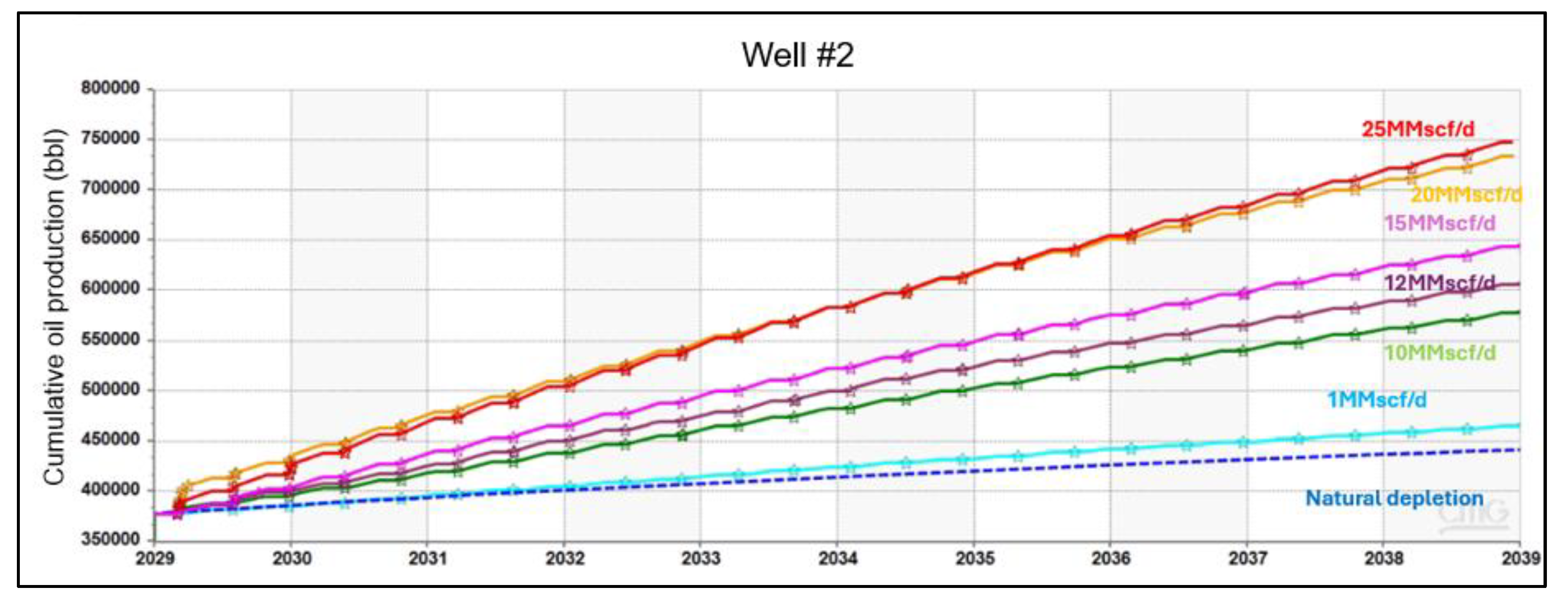
The cyclic time sensitivity analysis was derived from Case 1, with the injection rate varying from 1 MMscf to 25 MMscf per day, and the maximum bottom hole injection pressure was set at 7000 psi or 80% of fracture pressure to avoid any risk of formation integrity.
Error! Reference source not found. presents the oil production increments associated with various CO2 injection rates. Based on the simulation results, the cumulative oil production and estimated CO2 storage increase proportionally with the CO2 injection rate when the injection rate varies from 1 MMscf/d to 20 MMscf/d. In this range, the cumulative oil recovery rises from 6.3% to 68.8% as a result of the EOR process. Increasing the CO2 injection rate from 20 MMscf/d to 25 MMscf/d only boosts the increment by 0.5%. Therefore, the optimal injection rate was determined at 20 MMscf/d. At this rate, oil production reaches its highest incremental rate due to the CO2 huff-n-puff process, which also gives the highest CO2 storage efficiency. Moving above 20 MMscf/d injection rate increases operational costs and CO2 requirements without a proportional increase in oil production and estimated CO2 storage. This finding is also demonstrated in Error! Reference source not found., which shows that the cumulative oil increasing rate slows down significantly at the injection rate higher than 20 MMscf/d.
Table 8.
Effect of various CO2 injection rates on enhanced oil recovery.
| Scenario | Cumulative Oil Production | Cumulative CO2 | Estimated CO2 Storage (mil.lbs) |
||
|---|---|---|---|---|---|
| Total (STB) | Incremental EOR (STB) | Injection (mil.lbs) | Production (mil.lbs) | ||
| Primary depletion | 441,912 | Not applicable | |||
| 1MMscf/d | 469,891 | 27,979 | 87.51 | 66.52 | 20.99 |
| 7MMscf/d | 577,219 | 135,307 | 875.12 | 778 | 97.12 |
| 10MMscf/d | 605,789 | 163,877 | 1050.14 | 926.78 | 123.37 |
| 15MMscf/d | 643,661 | 201,749 | 1312.68 | 1143.17 | 169.51 |
| 20MMscf/d | 745,900 | 303,988 | 1742.00 | 1566.18 | 175.82 |
| 25MMscf/d | 748,371 | 306,459 | 1931.41 | 1733.94 | 197.47 |
Figure 19.
Cumulative oil production corresponding with different CO2 injection rates.
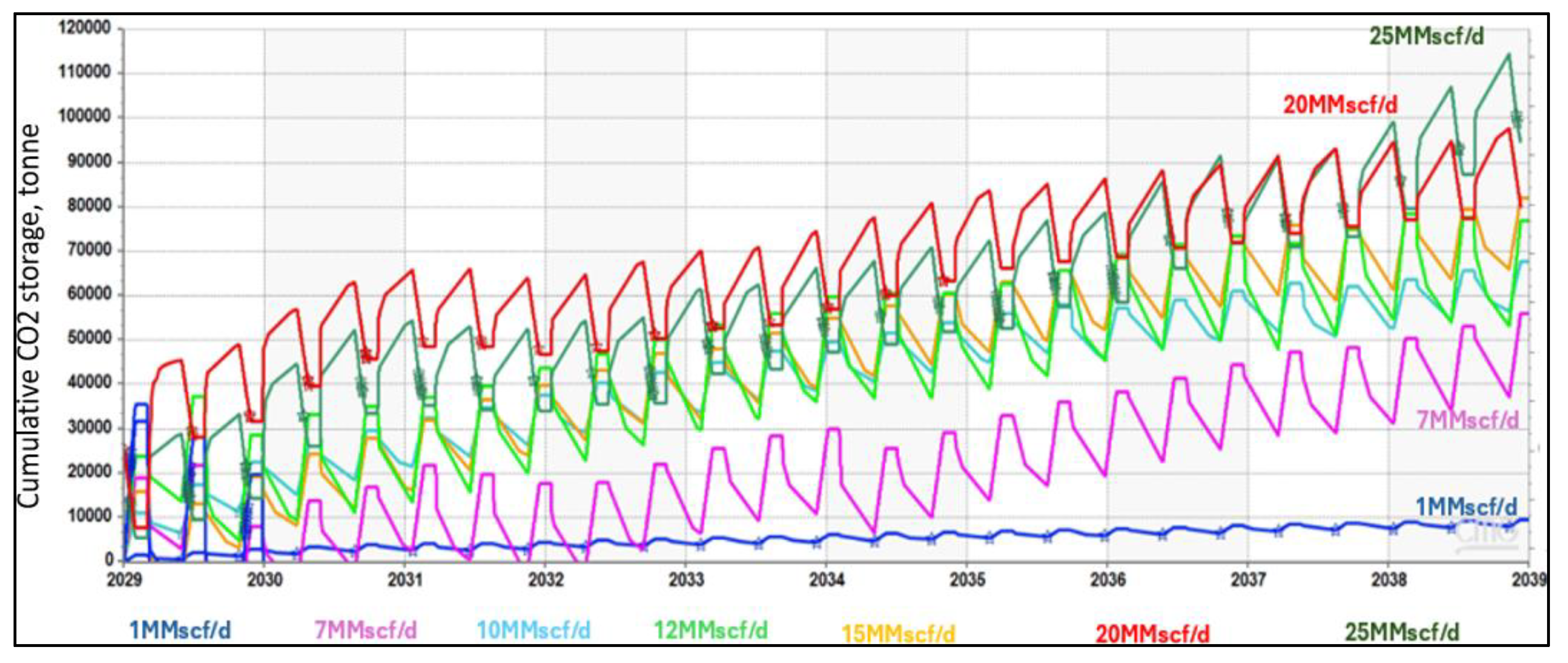
Error! Reference source not found. expresses the mass of CO2 storage corresponding with different CO2 injection rates. When the injection rate increases from 1 MMscf/d to 20 MMscf/d, the total amount of CO2 storage increases significantly from 10,000 to 80,000 tonnes over ten years. From 20 to 25 MMscf/d, the CO2 storage only increased by 10,000 tonnes. This observation emphasizes the importance of performing sensitivity analysis on the CO2 injection rate. By adopting these results, it is possible to optimize CO2 huff-n-puff operations, maximizing oil recovery while efficiently managing CO2 storage and operational costs.
Figure 20.
CO2 storage mass corresponding with various CO2 injection rates.
Error! Reference source not found. compares the CO2 mole fraction within the hydraulic fracture network under two different gas injection scenarios: 1 MMscf/d and 20 MMscf/d. The data clearly shows that with the higher injection rate of 20 MMscf/d, CO2 penetrates deeper and spreads more extensively throughout the fracture network and rock matrix. This deeper penetration facilitates better mixing with the residual oil in the reservoir. Consequently, the increased oil swelling observed in the 20 MMscf/d scenario enhances the efficiency of the production phase, thereby improving the oil recovery factor significantly.
Error! Reference source not found. andError! Reference source not found. illustrate the pressure distribution and reservoir pressure histogram after 10 years of CO2 injection for 1 MMscf/d and 20 MMscf/d scenarios, respectively. As depicted in Figure 22, at the conclusion of the injection period, the majority of the reservoir pressure remains below the MMP. This insufficient pressure results in lower oil recovery because CO2 does not mix well with the residual oil, failing to form a single miscible phase. In other words, at 1 MMscf/d, the CO2 remains largely immiscible, rendering it less effective in enhancing oil recovery.
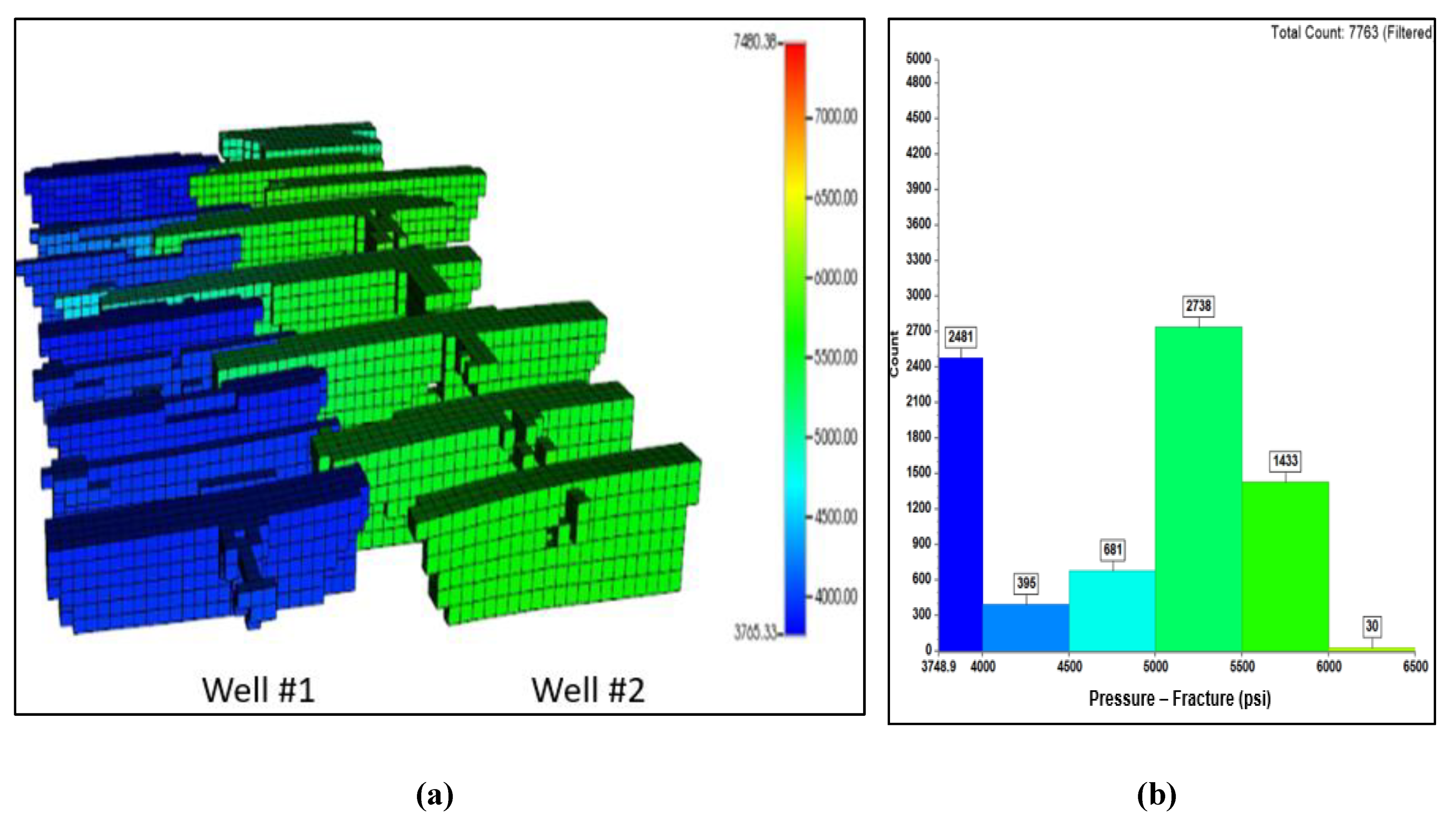
In contrast, Error! Reference source not found. demonstrates that with a 20 MMscf/d injection rate, most of the fracture network in Well #2 maintains a pressure above the MMP after 10 years of CO2 injection. This elevated pressure significantly enhances CO2 dispersion and mixing, leading to a remarkable improvement in the oil recovery factor, reaching up to 68.8%. Additionally, this higher injection rate proved effective in sequestering CO2 within the hydraulic fracture network and the depleted portions of the reservoir, further contributing to the efficiency and environmental benefits of the CO2 huff-n-puff process.
Figure 21.
(a) CO2 mole fraction in fracture network with 1 MMscf/d injection rate; (b) CO2 mole fraction in fracture network with 20 MMscf/d injection rate.
Figure 21.
(a) CO2 mole fraction in fracture network with 1 MMscf/d injection rate; (b) CO2 mole fraction in fracture network with 20 MMscf/d injection rate.
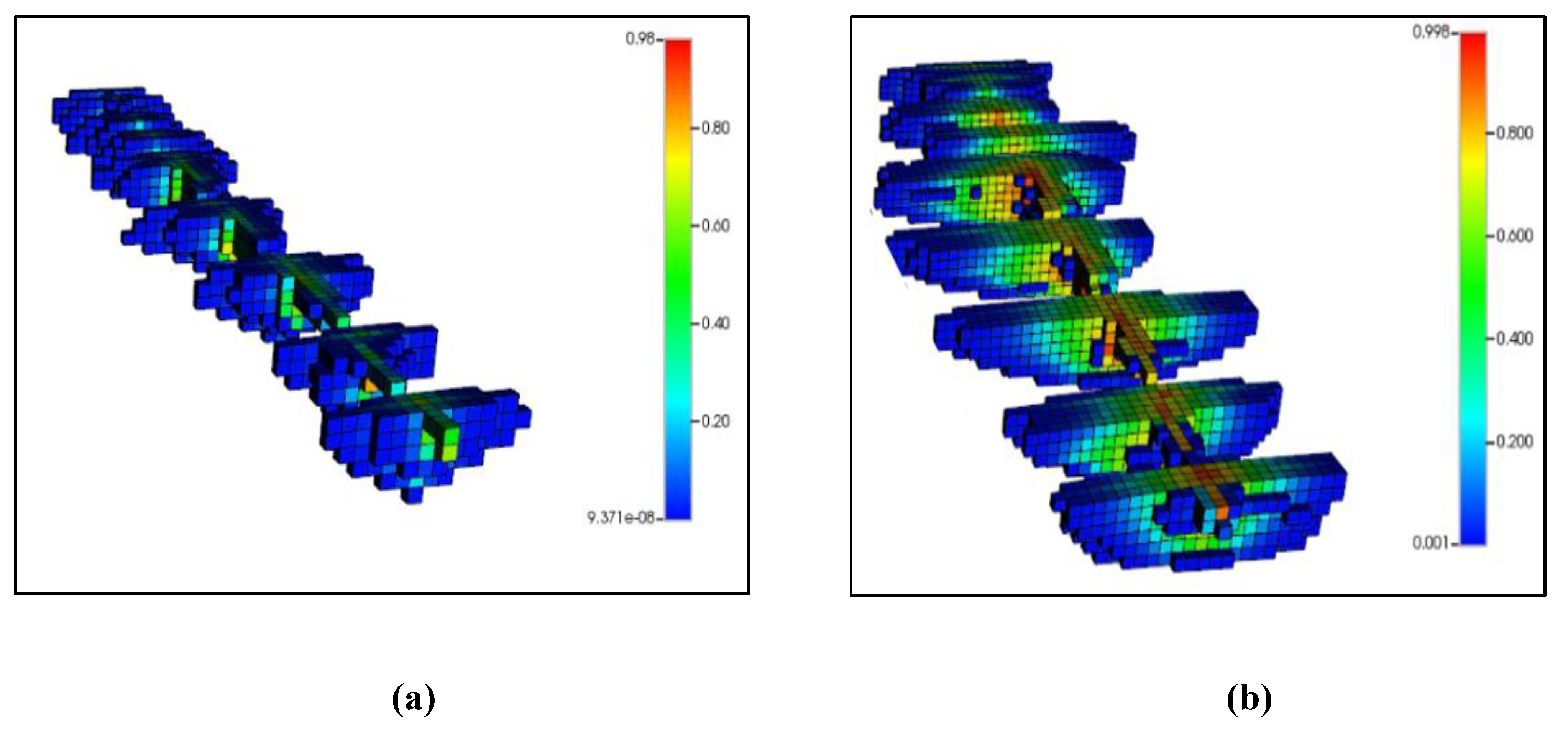
Figure 22.
(a) Pressure distribution after 10 years with 1 MMscf/d of CO2 injection; (b) Pressure histogram at the end of CO2 huff-n-puff simulation.
Figure 22.
(a) Pressure distribution after 10 years with 1 MMscf/d of CO2 injection; (b) Pressure histogram at the end of CO2 huff-n-puff simulation.
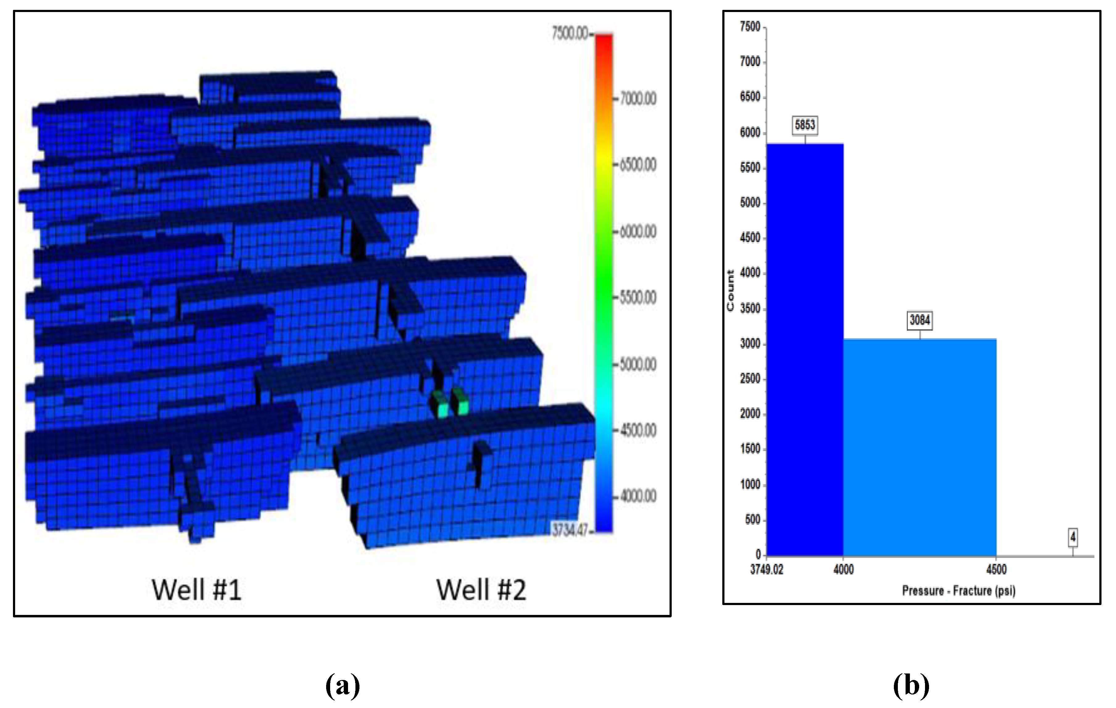
Figure 23.
(a) Pressure distribution after 10 years with 20 MMscf/d of CO2 injection; (b) Pressure histogram at the end of CO2 huff-n-puff simulation.
Figure 23.
(a) Pressure distribution after 10 years with 20 MMscf/d of CO2 injection; (b) Pressure histogram at the end of CO2 huff-n-puff simulation.
4. Discussion
Injection Rate and Performance Correlation
It was observed that higher injection rates correlate with increased oil recovery and CO2 storage. This positive correlation indicates that maximizing the injection rate, within operational limits, can lead to better overall performance in terms of oil recovery and CO2 sequestration. Since more CO2 can dissolve into brine at higher pressure, maintaining a high injection rate contributes to both economic and environmental benefits. Effective CO2 storage is crucial for reducing greenhouse gas emissions and meeting regulatory requirements. Moreover, maintaining reservoir pressure at or above the MMP at 4300 psi is essential for effective CO2 injection. Higher injection rates facilitate achieving this pressure more rapidly, enhancing CO2 dispersion throughout the hydraulic fracture network and rock matrix. Improved dispersion results in better oil mobilization and, consequently, higher recovery rates.
Operational Constraints
While higher injection rates are generally advantageous, they must be balanced against several operational limitations. First, CO2 supply is the most decisive factor related to the project’s continuity. It is essential to ensure that the chosen injection rate is sustainable, given the available CO2 supply. Second, the injection equipment must be able to handle the selected rate. Lastly, maximizing the injection rate should adhere to the maximum allowable injection pressure to avoid unintentionally fracturing the formation or equipment failure.
Optimization Strategy
Considering these factors, an optimized approach should include the following steps:
Step 1: Begin with the highest injection rate that the surface facilities can safely manage, without exceeding the maximum injection pressure.
Step 2: Closely monitor reservoir pressure to ensure it reaches and maintains a level at or slightly above the MMP.
Step 3: If the high injection rate is sustainable without issues, continue at that rate to maximize oil recovery and CO2 storage.
Step 4: If operational problems arise, such as CO2 supply limitations, gradually reduce the rate while closely monitoring performance metrics to maintain efficiency and effectiveness.
Leveraging the synthetic database generated through the simulation runs of this study, future research could focus on incorporating advanced machine learning techniques to further optimize CO2 huff-n-puff operations. The integration of machine learning can significantly reduce the computational costs associated with traditional reservoir simulations, enabling more efficient and faster decision-making processes [27]. Proxy models, which serve as simplified representations of complex reservoir simulations, can be developed using the extensive database created in this research. By employing various machine learning algorithms, these proxy models can facilitate the optimization of CO2 huff-n-puff processes.
5. Conclusions
The comprehensive simulation analysis to optimize the CO2 huff-n-puff process for enhanced oil recovery yielded significant and impactful findings. The study systematically investigated various CO2 injection rates, as well as different ratios of injecting, soaking, and producing times. Testing CO2 injection volumes ranging from 1 to 25 MMscf/d/well resulted in incremental oil recovery improvements from 6.3% to 69.3%.
By evaluating multiple combinations of cycle times, including injection, soaking, and production periods, the study identified the optimal cycle for maximizing oil recovery: 30 days of injection, 30 days of soaking, and 90 days of production. This finding highlights the critical role of the production phase in enhancing oil recovery using the CO2 huff-n-puff technique.
The optimized scenario for the pilot well, using a gas injection rate of 20 MMscf/d, demonstrated a remarkable 68.8% improvement in cumulative oil recovery compared to the natural depletion while efficiently sequestering approximately 80,000 tonnes of CO2 in the depleted hydraulic fractured network over ten years. This substantial enhancement in oil recovery and CO2 sequestration underscores the efficacy of the optimized CO2 huff-n-puff process in promoting oil recovery and reducing CO2 emissions.
This research presents a detailed workflow for implementing CO2 huff-n-puff in hydraulically fractured wells, aiming to maximize oil recovery through advanced numerical simulation and optimization. The workflow developed in this study enables a thorough and convenient assessment of the integrated operation’s feasibility, making it applicable to other unconventional plays in the U.S. besides the Wolfcamp formation in the Delaware Basin. Also, this approach can significantly aid in reservoir management and field development.
Furthermore, the study sets a precedent for future research and practical applications, demonstrating that an optimized CO2 huff-n-puff process can serve as a dual-purpose solution. It enhances hydrocarbon recovery from depleted fields and also contributes to environmental sustainability through effective CO2 sequestration. This dual benefit positions the CO2 huff-n-puff technique as an attractive option for enhanced oil recovery in hydraulically fractured horizontal wells.
Author Contributions
Conceptualization, Dung Bui; methodology, Dung Bui, Duc Pham, Son Nguyen, and Kien Nguyen; software, Dung Bui, Duc Pham, and Kien Nguyen; validation, Dung Bui, Duc Pham, and Kien Nguyen; formal analysis, Son Nguyen and Kien Nguyen; investigation, Dung Bui, Duc Pham, and Kien Nguyen; resources, Dung Bui and Duc Pham; data curation, Dung Bui, Duc Pham, Son Nguyen, and Kien Nguyen; writing—original draft preparation, Dung Bui, Duc Pham, Son Nguyen, and Kien Nguyen; writing—review and editing, Dung Bui, Duc Pham, Son Nguyen, and Kien Nguyen; visualization, Dung Bui; supervision, Dung Bui; project administration, Dung Bui and Duc Pham; funding acquisition, Dung Bui. All authors have read and agreed to the published version of the manuscript.
Funding
This research received no external funding.
Data Availability Statement
The original contributions presented in the study are included in the article, further inquiries can be directed to the corresponding author.
Conflicts of Interest
The authors declare no conflicts of interest.
References
- Ding, D. Y., Langouet, H., Jeannin L., “Simulation of fracturing-induced formation damage and gas production from fractured wells in tight gas reservoirs,” SPE Prod & Oper, vol. 28, pp. 246-258, 2013. [CrossRef]
- Guo, B., Gao, D., Quanjun W., “The Role of Formation Damage in Hydraulic Fracturing Shale Gas Wells,” in SPE Eastern Regional Meeting, Columbus, Ohio, USA, 2011. [CrossRef]
- Bottero, S., Picioreanu, C., Enzien, M., van Loosdrecht, M. C., Bruining, H., and Heimovaara, T., “Formation Damage and Impact on Gas Flow Caused by Biofilms Growing Within Proppant Packing Used in Hydraulic Fracturing,” in SPE International Symposium and Exhibition on Formation Damage Control, Lafayette, Louisiana, USA, 2010. [CrossRef]
- Khurshid, I., Al-Shalabi, E. W., Al-Attar, H., Ahmed K. A., “Characterization of Formation Damage and Fracture Choking in Hydraulically Induced Fractured Reservoirs Due to Asphaltene Deposition,” in SPE Gas & Oil Technology Showcase and Conference, Dubai, UAE, 2019. [CrossRef]
- Jeong, M. S., Lee, K. S., “Maximizing oil recovery for CO2 huff and puff process in pilot scale reservoir,” in World Congress on ACEM15, Icheon, Korea, 2015.
- Zhao, J., Wang, P., Yang, H., Tang, F., Ju, Y. and Jia, Y., “Experimental Investigation of the CO2 Huff and Puff Effect in Low-Permeability Sandstones with NMR,” ACS omega, vol. 6, no. 24, pp. 15601-15607, 2021. [CrossRef]
- Afari, S., Ling, K., Sennaoui, B., Maxey, D., Oguntade, T. and Porlles, J., “Optimization of CO2 huff-n-puff EOR in the Bakken Formation using numerical simulation and response surface methodology,” Journal of Petroleum Science and Engineering, vol. 215, p. 110552, 2022. [CrossRef]
- Song, C. and Yang, D., “Experimental and numerical evaluation of CO2 Huff and puff processes in Bakken formation,” Fuel, vol. 190, pp. 145-162, 2017. [CrossRef]
- Dohmen, T., Zhang, J., Blangy, J.P., “Measurement and Analysis of 3D Stress Shadowing Related to the Spacing of Hydraulic Fracturing in Unconventional Reservoirs,” in SPR Annual Technical Conference and Exhibition, Amsterdam, The Netherslands, 2014. [CrossRef]
- Dvory, N. Z., and Zoback, M. D., “Prior Oil and Gas Production Can Limit the Occurrence of Injection-Induced Seismicity: A Case Study in the Delaware Basin Of Western Texas and Southeastern New Mexico, USA,” Geology, vol. 49, no. 10, p. 1198–1203, 2011. [CrossRef]
- Hefner, W. and Davudov, D., “Field Development Using Compositional Reservoir Simulation and Uncertainty Analysis in the Delaware Basin,” in SPE Oklahoma City Oil and Gas Symposium, Oklahoma City, Oklahoma, USA, 2019. [CrossRef]
- D. Bui, “Geomechanics-reservoir Coupled Simulation For Well Spacing Optimization in Eddy County in Delaware Basin, New Mexico. Doctoral dissertation, New Mexico Institute of Mining and Technology,” New Mexico Institute of Mining and Technology, 2023.
- Bandis, S.C., Lumsden, A.C. and Barton, N.R., “Fundamentals of rock joint deformation,” International Journal of Rock Mechanics and Mining Sciences & Geomechanics Abstracts, vol. 20, no. 6, pp. 249-268, 1983. [CrossRef]
- Bui, D., Nguyen, T., Nguyen, T. and Yoo, H., “Formation Damage SImulation of a Multi-fractured Horizontal Well in a Tight Gas/Shale Oil Formation,” Journal of Petroleum Exploration and Production Technology, vol. 13, no. 1, pp. 163-184, 2023. [CrossRef]
- Gaswirth, S.B., Marra, K.R., Lillis, P.G., Mercier, T.J., Leathers-Miller, H.M., Schenk, C.J., Klett, T.R., Le, P.A., Tennyson, M.E., Hawkins, S.J. and Brownfield, M.E., “Assessment of undiscovered continuous oil resources in the Wolfcamp shale of the Midland Basin, Permian Basin Province, Texas,” US Geological Survey, vol. 3092, 2016. [CrossRef]
- Nguyen, S.T., Nguyen, T.C., Yoo, H. and El-kaseeh, G., “Geomechanical Study and Wellbore Stability Analysis for Potential CO2 Storage into Devonian and Silurian Formations of Delaware Basin,” in SPE Oklahoma City Oil and Gas Symposium., Oklahoma City, Oklahoma, USA, 2023. [CrossRef]
- EIA, “Permian Basin Part.1: Wolfcamp, Bone Spring, Delaware Shale Plays of the Delaware Basin,” US Energy Information Administration Report, 2020.
- Bui, D., Nguyen, S., Nguyen, T., and H. Yoo., “The Integration of Geomechanics and Reservoir Modeling for Hydraulic Fracturing and Well Spacing Optimization in the Third Bone Spring Sand of the Delaware Basin,” in SPE Eastern Regional Meeting, Wheeling, West Virginia, USA, 2023b. [CrossRef]
- Nguyen, S. T., Hoang, S. K., Khuc, G. H. and Tran, H. N., “Pore Pressure and Fracture Gradient Prediction for the Challenging High Pressure and High Temperature Well, Hai Thach Field, Block 05-2, Nam Con Son Basin, Offshore Vietnam: A Case Study,” in In SPE/IATMI Asia Pacific Oil & Gas Conference and Exhibition. OnePetro., 2015. [CrossRef]
- Nguyen, S. T., Hoang, S. K. and Khuc, G. H., “Improved Pre-Drill Pore Pressure Prediction for HPHT Exploration Well Using 3D Basin Modeling Approach, a Case Study Offshore Vietnam,” in Paper SPE-28606-MS presented at the Offshore Technology Conference Asia, Kuala Lumpur, Malaysia, 2018. [CrossRef]
- Nguyen, S., Nguyen, T., Tran, H. and Ngo, Q., “Integration of 3D Geological Modeling and Fault Seal Analysis for Pore Pressure Characterization of a High Pressure and High Temperature Exploration Well in Nam Con Son Basin, a Case Study Offshore Vietnam,” in In International Petroleum Technology Conference. OnePetro., 2021. [CrossRef]
- Hoang, S.K., Nguyen, S.T., Khuc, G.H., Nguyen, D.A. and Abousleiman, Y.N., “Overcoming Wellbore Instability Challenges in HPHT Field with Fully Coupled Poro-Thermo-Elastic Modeling: A Case Study in Hai Thach Field Offshore Vietnam,” in In Offshore Technology Conference Asia. OnePetro., 2016. [CrossRef]
- Snee, J. L., and Zoback, M. D., “State of Stress in the Permian Basin, Texas and New Mexico: Implications for Induced Seismicity,” The Leading Edge, vol. 37, pp. 127-134, 2018. [CrossRef]
- Bui, D., Nguyen, T., Yoo, H. , “A Coupled Geomechanics-Reservoir Simulation Workflow to Estimate the Optimal Well-Spacing in the Wolfcamp Formation in Lea County,” in AADE 2023 National Technical Conference & Exhibition, Midland, Texas, 202. [CrossRef]
- Ojha, S.P., Misra, S., Tinni, A., Sondergeld, C. and Rai, C., “Relative permeability estimates for Wolfcamp and Eagle Ford shale samples from oil, gas and condensate windows using adsorption-desorption measurements,” Fuel, vol. 208, pp. 52-64, 2017. [CrossRef]
- Ginting, M., Wijayanti, P. and Cindra, R.A., “CO2 MMP determination on L Reservoir by using CMG simulation and correlations,” Journal of Physics: Conference Series, vol. 1402, no. 05, p. 055107, 2019. [CrossRef]
- You, J., Ampomah, W., Morgan, A., Sun, Q., Huang, X., “A comprehensive techno-eco-assessment of CO2 enhanced oil recovery projects using a machine-learning assisted workflow,” International Journal of Greenhouse Gas Control, vol. 111, no. 1750-5836, 2021. [CrossRef]
Disclaimer/Publisher’s Note: The statements, opinions and data contained in all publications are solely those of the individual author(s) and contributor(s) and not of MDPI and/or the editor(s). MDPI and/or the editor(s) disclaim responsibility for any injury to people or property resulting from any ideas, methods, instructions or products referred to in the content. |
© 2024 by the authors. Licensee MDPI, Basel, Switzerland. This article is an open access article distributed under the terms and conditions of the Creative Commons Attribution (CC BY) license (http://creativecommons.org/licenses/by/4.0/).
Copyright: This open access article is published under a Creative Commons CC BY 4.0 license, which permit the free download, distribution, and reuse, provided that the author and preprint are cited in any reuse.


