Submitted:
11 July 2024
Posted:
12 July 2024
You are already at the latest version
Abstract
Abstract: Flexible pressure sensors are electronic devices that can be attached to various irregular surfaces to measure the pressure. It is widely used in wearable devices and for health detection. In this study, a general carbon nanotubes/polydimethylsiloxane (CNTs/PDMS) sponge electrode was fabricated as the elementary component of the compressible system. The sensitivity of the flexible pressure sensor is improved by optimizing the preparation process of the conductive sponge and surface modification of the CNTs, and the highest sensitivity reached 71.831 kPa-1(0~2 kPa). The flexible pressure sensor can be used to detect subtle pressure quickly and accurately so that it can be used as wearable sensor to measure the radial artery wave of a human body, which has potential applications in health care and other fields.
Keywords:
CNTs
; Ag
; PDMS sponge
; pressure sensitivity
; wearable
1. Introduction
With the rapid development of electronic and wireless communication technology, as the only bridge linking the external environment with the internal intelligent system, the flexible pressure sensor has gradually become a new research hotspot [1,2,3]. At the same time, with the increasing attention paid to people health problems, flexible wearable pressure sensors used to detect human physiological signals have become very promising [4,5]. Based on the characteristics of the human body, wearable pressure sensors can be characterized by light weight, portability and high sensitivity.
A flexible piezoresistive pressure sensor is a typical sensor that converts external pressure into a resistance signal among various sensors that detect human motion and monitor health conditions [6,7]. Owing to its manufacturability and simple structure, it is widely used in wearable devices [8,9,10]. The conductive porous sponge is considered a new type of piezoresistive material that can replace the traditional piezoresistive material owing to the synergistic effect of the high electrical conductivity of its filled material and the excellent compression-recovery performance of the porous stent [11,12]. Presently, pressure sensors with a certain flexibility prepared by chemical vapor deposition or carbonization processes using piezoresistive pressure sensors based on spongy materials have high sensitivity and low strain detection capability [13,14], which meet the demands of wearable applications. However, low integration and complex micro/nano processing techniques are needed to solve urgently [15,16].
Additionally, owing to the large contact resistance between CNTs and easy agglomeration, the sensitivity of the CNTs/polymer flexible pressure sensor is low, and the measurement threshold is high, thus it is impossible to measure the signal change under a slight pressure and it is difficult to apply in wearable equipment [17,18,19]. Modifying the surface of CNTs, loading metal or metal oxide particles to prepare a metal/metal oxide-CNT composite conductive filler material can improve the performance of CNTs and reduce the contact resistance between CNTs [20,21,22], so as to prepare a flexible pressure sensor with excellent performance.
Therefore, using CNTs and PDMS as the main research carriers for flexible pressure sensors, utilizing the high conductivity of CNTs and the flexible properties of PDMS to prepare a high-performance flexible pressure sensor has a very good research prospect, not only improving the sensor's conductive properties [23,24], but also because PDMS has good biocompatibility [25], it can play an important role in bionic electronic skin. At the same time, the Ag-CNTs/PDMS flexible pressure sensor was prepared by surface modification of the CNTs, which exhibited excellent sensing performance. The CNTs/PDMS conductive sponge is a new type of flexible piezoresistive conductive material that can replace traditional piezoresistive materials [27,28]. It is expected to be applied in emerging fields such as smart wearable devices and has important practical significance.
2. Materials and Methods
2.1. Fabrication of PDMS Sponge
First, the elastomer and crosslinker of commercial PDMS (PDMS: Sylgad 184, Dow Corning Co.) were mixed in a ratio of 10:1. Subsequently, the air bubbles in the PDMS prepolymer were removed using a vacuum dryer, and the PDMS was squeezed into the sugar using a circulating water multipurpose vacuum pump. The pore size and porosity were determined based on the granularity of the sugar. The sugar-PDMS mixture was put in a drying box and cured at 80 ℃ for 3 hours. Finally, the cured sugar-PDMS mixture was dissolved in water at 40 C, and dried.
2.2. Fabrication of Ag-CNTs Composite
First, 400 mg of CNTs were placed in a beaker containing H2SO4 and HNO3 100 ml (volume ratio 3:1). Then, the beaker was placed in an ultrasonic cleaner with an initial water temperature of 80 °C water for 2 h, and after the acidification was completed, the solution was washed with water to neutrality. And 6.8 g AgNO3 powder was dissolved in aqueous solution of 50 ml (need to protect from light). At the same time, the beaker was stirred constantly using the magnetic stirrer, and ammonia water was added to the clarification continuously (the solution turned turbid by transparency and then became transparent). The silver-ammonia solution was added to a well-saturated CNTs solution, and the pH of the solution was adjusted to a predetermined range (pH: 8~11). 12 mL of hydrazine hydrate solution was added as a reducing agent to perform a plating reaction for 20 minutes. Finally, after the reduction was completed, the temperature was lowered and the supernatant liquid was poured out. The precipitate then washed with deionized water to neturality.
2.3. Fabrication of Conductive Sponge
Figure 1 shows the fabrication process of conductive sponges for pressure sensors. CNTs and Ag-CNTs were selected as conductive fillers, which were loaded onto the PDMS sponge substrate by the dip-drying method (drying methods are divided into freeze-drying and heat-drying), and by changing the number of extrusions to obtain conductive sponges with weight ratio (wt%) of different conductive filler materials (wt%=0.5, 1.0, 1.5, 2.0, 2.5, 3.5 and 5.0).
2.4. Fabrication of Flexible Pressure Sensors
First, two pieces of conductive glass (ITO) were selected and the film on the conductive surface was removed. Then, two conductive copper films were connected to ITO conductive glass to prepare a conductive electrode. Finally, the prepared conductive electrodes were used to cover the upper and lower surfaces of the conductive sponge to prepare a flexible pressure sensor.
3. Results
3.1. Characterization of CNTs Conductive Sponges and Ag-CNTs Particles
The surface topography of the Ag-CNTs/PDMS conductive sponges and Ag-CNTs particles was determined from the cross-sectional images obtained using field emission-scanning electron microscopy (FE-SEM; S-4800, Hitachi), as shown in Figure. 2. As illustrated in Figure 2(a), The PDMS sponge had a cross-linked network structure and the CNTs were successfully loaded onto the flexible PDMS substrate. As illustrated in Figure 2(b), the cross-linking of CNTs was distributed in the conductive sponge, and agglomeration of CNTs appeared in the local area. As illustrated in Figure 2(c), the Ag-CNTs were successfully loaded onto the flexible PDMS substrate. As illustrated in Figure 2(d), the silver particles wrapped the CNTs such that the CNTs existed in a conductive sponge in the form of spherical particles. Owing to the coating of the silver particles, the conductive sponges were transformed from being in direct contact with each other between the CNTs to contact the silver particles. As illustrated in Figure 2(e)~(f), after being coated with silver, the original smooth surface of the CNTs became rough and uneven.
3.2. Sensitivity of CNTs/PDMS Flexible Pressure Sensors (Heat-Drying)
On the one hand, with high compressibility and electronic conductivity, the CNTs/PDMS conductive sponge can detect various strains as well. In particular, the compressive stress mediate the conductive pathway of the CNTs/PDMS conductive sponge under different strains, resulting in conductance modulation. In Figure 3, the red dot represents the contact point of the conductive pathway, the red line represents the assumed conductive pathway, and the black object represents the CNTs/PDMS conductive sponge. Figure 3 (a) shows a schematic of the contact point of the conductive pathway in a conductive sponge under an uncompressed state. It was found that the internal connection of the conductive sponge was not yet stable in the initial state, and the number of contact points was small, thus the interior conductive pathway of the conductive sponge was less, and the conductive sponge had a higher resistance at this time. As shown in Figure 3(b), when the conductive sponge was compressed by external pressure, the number of contact points increased rapidly, which caused the conductive pathway increase rapidly and the resistance of the conductive sponge decreases gradually. Because the electron transfer rate is faster at this time, the response rate of the entire flexible pressure sensor increases.
The resistance response can be monitored using a voltage signal with the stress imposed on the top surface during the compression. The resistance response is defined ΔR/R0 = (R0 – RP)/R0, where R0 and RP represent the resistances without and with compressive stress, respectively. As shown in Figure 4, when the weight ratio of CNTs is in the range of 0.5 wt% to 2.5 wt%, as the proportion of CNTs increased, the resistance change rate increased gradually under the same pressure, but when the weight ratio exceeds 2.5 wt%, as the proportion of CNTs increased, the resistance change rate decreased gradually under the same pressure. This is because when the CNTs content is 0.5 wt% ~ 2.5 wt%, the PDMS sponge has not yet reached the saturation state. With an increase in the weight ratio of CNTs, the conductive channel in the conductive sponge gradually increased. When the CNTs content was more than 2.5 wt%, the PDMS sponge reached a saturation state. Further filling of the CNTs causes twining between the CNTs, which reduces the performance of CNTs in the conductive sponge.
The stress sensitivity of S can be defined as the slope of the curves:
The sensitivity S is the change in the resistance change rate of the sensor under the condition of 1kPa change in pressure. Figure 4 shows the sensitivity fitting of the CNTs/PDMS flexible pressure sensors with weight ratios of 0 to 2 kPa, 3 to 10 kPa, and 15 to 40 kPa. As shown in this figure, when the weight ratio of the CNTs is in the range of 0.5 wt%~2.5 wt%, the sensitivity increases gradually with an increase in the weight ratio. When the weight ratio was 2.5 wt%, the sensitivity reached at peak value of 31.298 kPa-1, and the sensitivity gradually began to decrease with an increase in the weight ratio. At the same time, by comparing the sensitivity of 0~2 kPa, 3~10 kPa and 15~40 kPa, it was found that the sensitivity decreased with increasing the pressure. The reason is that in the stage of the initial pressure, the inside of the conductive sponge is relatively loose and the Poisson is relatively large, so that the conductive sponge can produce larger deformation under the action of low pressure, which causes the conductive path inside the conductive sponge increase rapidly so that the sensitivity increases.
3.3. Sensitivity of CNTs/PDMS Flexible Pressure Sensors (Freeze-Drying)
As shown in Figure 5(a)~(b), when the weight ratio of CNTs is in the range of 0.5 wt% to 3.5 wt%, as the proportion of CNTs increases, the resistance change rate increases gradually under the same pressure, but when the weight ratio exceeds 3.5 wt%, as the proportion of CNTs increases, the resistance change rate decreases gradually under the same pressure. As shown in Figure 5(c)~(i), when the weight ratio of the CNTs is in the range of 0.5 wt%~3.5 wt%, the sensitivity increases gradually with an increase in the weight ratio. When the weight ratio is 3.5 wt%, the sensitivity reached at peak value of 41.651 kPa-1, and gradually began to decrease with an increase in the weight ratio.
3.4. Sensitivity of Ag-CNTs/PDMS Flexible Pressure Sensors
As shown in Figure 6(a), when the weight ratio of Ag-CNTs was in the range of 0.5 wt% to 5.0 wt%, as the proportion of CNTs increased, the resistance change rate increased gradually under the same pressure. As shown in Figure 6(b)~(h), when the weight ratio of the Ag-CNTs is in the range of 0.5 wt%~5.5 wt%, the sensitivity increases gradually with the increase of the weight ratio. When the weight ratio was 5.0 wt%, the sensitivity reached at peak value of 71.831 kPa-1.
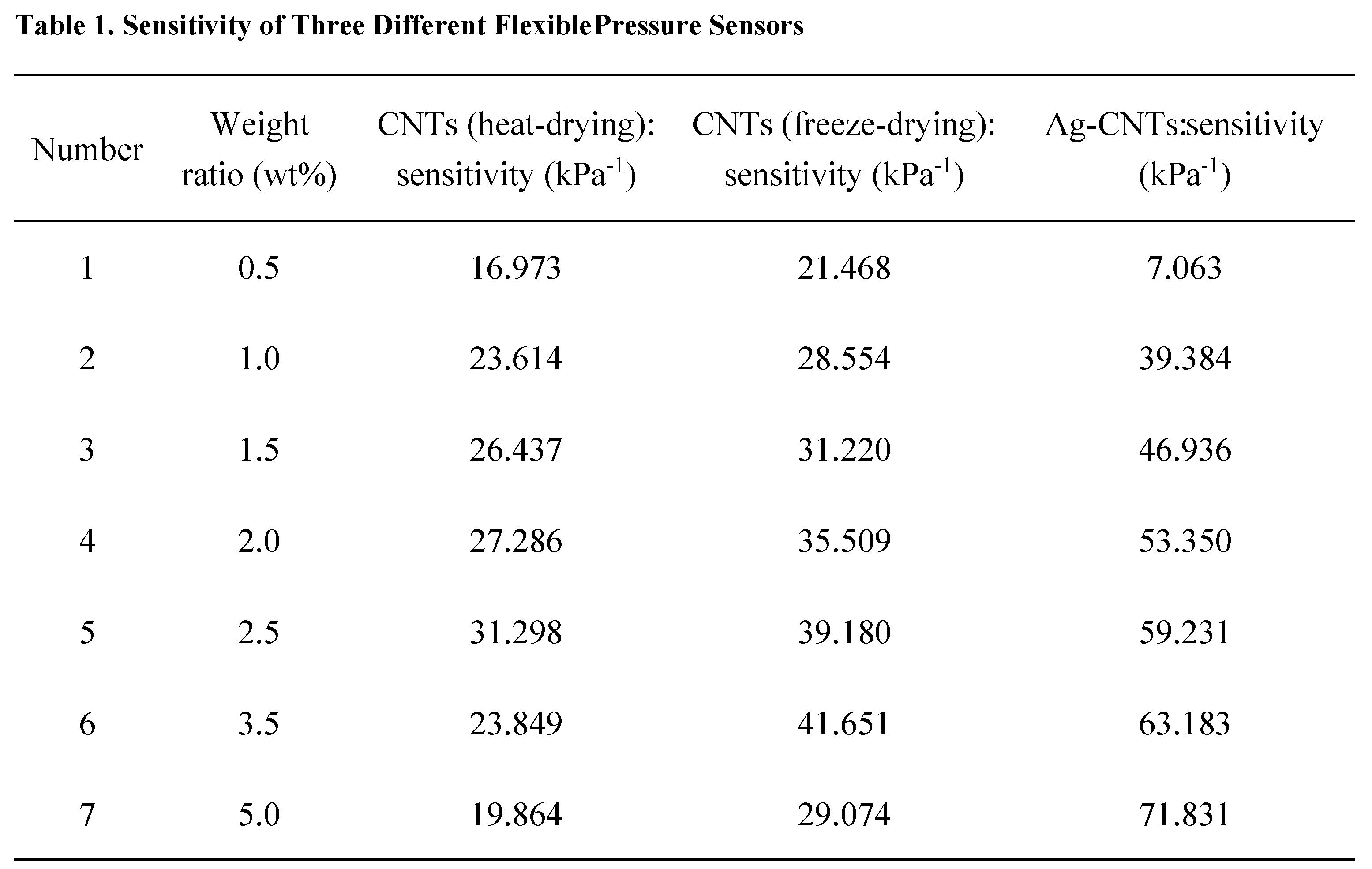
The sensitivities of the CNTs/PDMS flexible pressure sensors (heat-drying and freeze-drying) and Ag-CNTs/PDMS flexible pressure sensors in the pressure range of 0~2 kPa were compared. The comparison values are listed in Table 1 and a comparison chart is shown in Figure 7. As shown in Figure 7(a), the CNTs/PDMS flexible pressure sensor prepared by freeze-drying has a higher sensitivity than the CNTs/PDMS flexible pressure sensor prepared by heat-drying and the sensitivity of Ag-CNTs/PDMS flexible pressure sensor is much higher than that of the CNTs/PDMS flexible pressure sensor when the weight ratio of the conductive filler material exceeds 0.5 wt%. In summary, it can be found that by optimizing the preparation process of the conductive sponge and the surface modification of the CNTs, the sensitivity of the flexible pressure sensor can be improved, so that the sensor has more excellent performance.
3.5. Stability and Hysteresis of the Flexible Pressure Sensor
(1) Stability
For the overall measurements, the resistance responses to repeated compression and release cycles are illustrated in Figure 7(a). The flexible pressure sensor exhibited good stability in the overall cycle test under three different pressures, and the resistance change rate gradually increased as the pressure increased. Even with slight fluctuations under the test conditions at a pressure of 1 kPa, it is basically stable. Additionally, for large repeated strains, a series of resistance responses were obtained, as shown in Figure 7(b). For different compressive strains, a higher strain results in a larger resistance response intensity.
(2) Hysteresis
Hysteresis refers to the degree of resistance change-pressure curve misalignment during the reverse and positive trip of the sensor. During the experiment, we developed a flexible pressure sensor with a complete load application and load release process to detect the rate of resistance change. The effect of hysteresis is crucial for sensors to detect dynamic loads. A large hysteresis in the flexible pressure sensor leads to irreversible recovery during the measurement of the dynamic load, thus affecting the accuracy of the experimental results. As shown in Figure. 7(c)~(e), the hysteresis error is larger at the low pressure stage and the hysteresis error is smaller at the higher pressure stage. This is because when the pressure is small, a small pressure change causes a large deformation of the conductive sponge, and it is more difficult for the conductive sponge to quickly return to the initial position, which leads to the larger hysteresis error. With a continuous increase in pressure, the conductive sponge exhibited a smaller deformation and the hysteresis error decreased gradually. The maximum hysteresis error of the flexible pressure sensor with an Ag-CNTs content of 2.5wt% was 9.45%. The maximum hysteresis error of the flexible pressure sensor with an Ag-CNTs content of 3.5 wt% was 5.74%. When the pressure exceeded 15 kPa, the hysteresis error between the reverse and positive trips was essentially zero, and the coincidence degree of the resistance change rate pressure curve was good. The maximum hysteresis error of the flexible pressure sensor with an Ag-CNTs content of 5.0 wt% is 3.39%, and when the pressure exceeds 10 kPa, the reverse and positive trip curves coincide.
3.6. Temperature-Pressure Coupling Applications of Flexible Sensor
(1) Temperature static characteristics of the flexible sensor
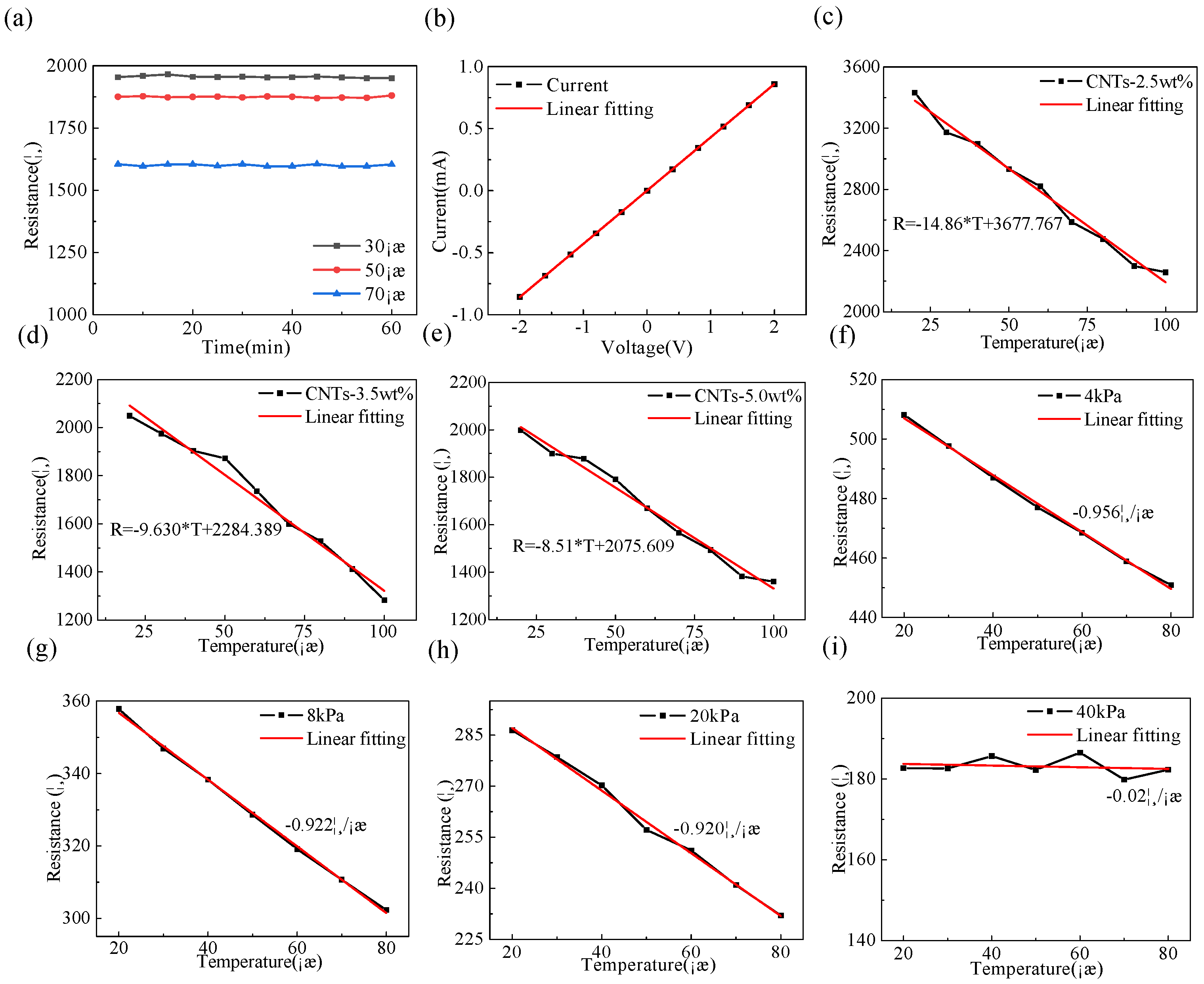
As shown in Figure 8(a), the fluctuation in the resistance of the sensor is very small at different temperatures, indicating that the sensor has good stability and can be used for the coupling test of temperature and pressure. When a flexible sensor is tested, it is necessary to apply a certain voltage to the flexible sensor, so that self-heating can occur. Because the self-heating generated by the instrument may affect the subsequent temperature test so that it can produce errors, it is necessary to exclude the influence of self-heating on the temperature test. As shown in Figure 8(b), the fitted I-V curves have a high degree of coincidence, and the resistance of the sensor does not vary with the voltage. The influence of self-heating generated by applying voltage on the temperature test was almost negligible, thus the flexible pressure sensor could be used for the temperature sensing test.
(2) Temperature sensing performance of the flexible sensor
As shown in Figure 8(c)~(e), the sensors with three different CNTs contents show a linearly decreasing trend (NPC effect: negative temperature coefficient) as the temperature rises at a temperature gradient of 20~100 °C. This is because an increase in temperature increases the probability of electron transition between CNTs so that the resistance of the sensor decreases. The temperature-resistance formula was obtained by linearly fitting the three curves, and then the temperature sensitivity coefficient (TCR) was calculated according to the following formula:
R_T=R_0×(1+TCR×T)
In this formula, TCR is the temperature sensitivity coefficient, R0 is the initial resistance, and T is the ambient temperature. According to the calculation, the temperature sensitivity coefficient (TCR) of the flexible sensor can be maintained at approximately -0.00410 °C-1, indicating good stability. This indicates that the prepared sensor is expected to realize the temperature sensing function of the bionic human skin.
(3) Coupling of temperature and pressure
As shown in Figure 8(f)~(i), when the pressure is 4, 8 and 20 kPa, the resistance decreases linearly with the increase in temperature. When the pressure was 40 kPa, the resistance remained unchanged, and was not affected by temperature changes. This is because when the pressure is low, the conduction network inside the conductive sponge changes with an increase in temperature. When the pressure exceeded a certain range, the conductive network inside the conductive sponge was shaped. The phenomenon of electronic transition is hardly observed in CNTs, so the temperature does not affect the resistance of the conductive sponge. By linearly fitting the temperature test curves under the four different pressures, the linear slope of each curve is the temperature coefficient. The result shows that within a certain pressure range, the temperature coefficient (the slope of the fitting curve) remains at -0.900 Ω/°C, therefore, the coupling formula of pressure and temperature can be proposed as follows:
when SP is the sensitivity, KT is the temperature coefficient, R0 is the initial resistance of the conductive sponge, ∆P and ∆T are the changes in the pressure and temperature, respectively. The sensor can simulate the sensing function of human skin to sense temperature and pressure, while simultaneously measuring the environmental temperature and the external force acting on the sensor.
Figure 9.
(a) Preparation sketch of pulse pressure sensor. (b) Schematic diagram of pulsed measurement. Pulse pulsation (c) 15 seconds in normal condition (d) 15 seconds after exercise (e) 1 minute in normal condition (f) 1 minute after exercise.
Figure 9.
(a) Preparation sketch of pulse pressure sensor. (b) Schematic diagram of pulsed measurement. Pulse pulsation (c) 15 seconds in normal condition (d) 15 seconds after exercise (e) 1 minute in normal condition (f) 1 minute after exercise.
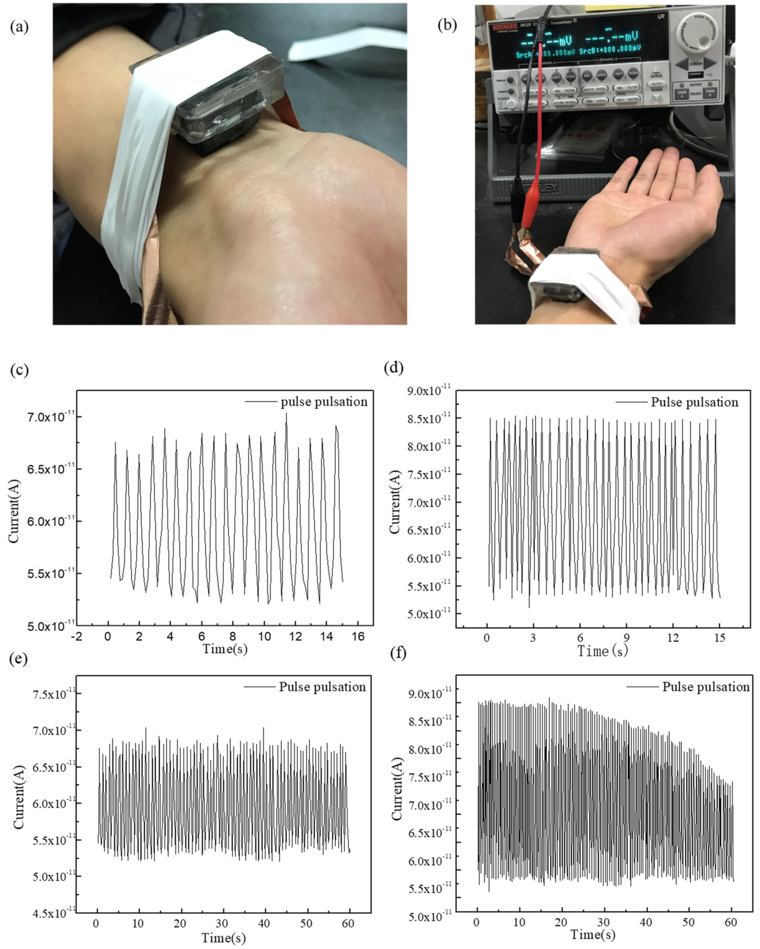
3.7. Application of Wearable Pulse Sensing Device
Through the above experiment, we found that the prepared flexible pressure sensor has the function of detecting tiny pressures, therefor, it is assembled into a wearable pulse sensor device. We set up the prepared pulse sensor device on the wrist with an adhesive tap and set the time for 15s and 1 min to measure the change in current with pulse beat, as shown in Figure 9(a)~(b). Figure 9 (c)~(d) show the pulse beats in two different states within 15s, where each crest represents a pulse beat. It can be observed that the pulse beating curve in the motion state is denser and higher in peak, which conforms to the actual situation. Figure 9(e)~(f) show the pulse beats in two different states within 1 min. According to the curve, the number of pulse beats per minute during the normal state of the tester was 76, and the number of beats per minute after the exercise increased to 119 beats. At the same time, we found that in the pulse beat curve after exercise, the peak value at the beginning was higher and the distribution of the peaks was denser. As time passes, the peak value gradually decreases and the peak distribution gradually disperses. This is because human physiological conditions tend to stabilize during testing. These results confirm the satisfactory capability of the wearable pulse device to identify the pulse condition of the human body in different states.
4. Conclusions
In summary, a flexible pressure sensor based on a CNTs/PDMS conductive sponge is proposed. A sponge-like PDMS substrate was synthesized using sugar as a template. This method is simple effective and it can be produced in large quantities. By combining CNTs with PDMS sponges using dip-drying method, porous structure CNTS/PDMS sponges with high electrical conductivity and excellent compression-recovery properties were prepared. On one hand, by optimizing the preparation process of the flexible pressure sensor, it was found that the flexible pressure sensor prepared using the freeze-drying method had higher sensitivity than the heat-drying method. On the other hand, the Ag-CNTs/PDMS flexible pressure sensor was prepared by surface modification of CNTs. The sensor has a higher sensitivity, lower detection limit and reliable response signals under repeated compressive stress (the sensitivity is 71.831 kPa-1, and the minimum detection limit is 0.25kPa). Because the prepared sensor can be used to detect the temperature, the CNTs/PDMS flexible pressure sensor was applied to measure the temperature and pressure simultaneously, and the coupling relation between temperature and pressure in a certain pressure range was obtained, which can simulate the skin's perception of temperature and pressure. Furthermore, taking advantage of the high sensitivity of the Ag-CNTs/PDMS flexible pressure sensor, it can be prepared as a wearable pulse sensor device that can detect physiological characteristics of different states (such as pulse, etc.). It is expected to be applied in medical detection and other applications.
Author Contributions
Conceptualization, S.D. and Y.P.; methodology, S.D. and Y.P.; validation and formal analysis, S.D.; investigation S.D.; data curation and writing— original draft preparation, S.D.; writing—review, editing supervision, and Y.P. All authors have read and agreed to the published version of the manuscript.
Funding
This research was funded by, grant number and “The APC was funded by XXX”. Check carefully that the details given are accurate and use the standard spelling of funding agency names at https://search.crossref.org/funding. Any errors may affect your future funding.
Acknowledgments
The authors are grateful to the National Natural Science Foundation of China (Grant No. 51905090). The authors are also grateful for the insightful discussions and continuous support from Ruling Chen, Yanzhu Yang, Caihong Ding, Yao Huang, and Haojie Lang (Donghua University).
Conflicts of Interest
The authors declare no conflicts of interest.
References
- Liu L, Yu Y, Yan C, et al. Wearable energy-dense and power-dense supercapacitor yarns enabled by scalable graphene-metallic textile composite electrodes.[J]. Nature Communications, 2015, 6:7260. [CrossRef]
- AHN B Y, DUOSS E B, MOTALA M J, et al. Omnidirectional Printing of Flexible, Stretchable, and Spanning Silver Microelectrodes [J]. Science, 2009, 323(5921): 1590-1593. 10.1126/science.116837.
- SON Y, YEO J, MOON H, et al. Nanoscale Electronics: Digital Fabrication by Direct Femtosecond Laser Processing of Metal Nanoparticles [J]. Advanced Materials, 2011, 23(28): 3176-3181. [CrossRef]
- HAMMOCK M L, CHORTOS A, TEE B C K, et al. 25th Anniversary Article: The Evolution of Electronic Skin (E-Skin): A Brief History, Design Considerations, and Recent Progress [J]. Advanced Materials, 2013, 25(42): 5997-6037. [CrossRef]
- Kim J, Lee M, Shim H J, et al. Stretchable silicon nanoribbon electronics for skin prosthesis.[J]. Nature Communications, 2014, 5(5):5747. [CrossRef]
- Wu N, Cheng X, Zhong Q, et al. Cellular Polypropylene Piezoelectret for Human Body Energy Harvesting and Health Monitoring[J]. Advanced Functional Materials, 2015, 25(30):4788-4794. [CrossRef]
- Zhang X S, Su M, Brugger J, et al. Penciling a triboelectric nanogenerator on paper for autonomous power MEMS applications[J]. Nano Energy, 2017, 33:393-401. [CrossRef]
- Gong S, Schwalb W, Wang Y, et al. A wearable and highly sensitive pressure sensor with ultrathin gold nanowires[J]. Nature Communications, 2014, 5(2):3132. [CrossRef]
- Jung S, Kim J H, Kim J, et al. Reverse-micelle-induced porous pressure-sensitive rubber for wearable human-machine interfaces.[J]. Advanced Materials, 2014, 26(28):4825-30. [CrossRef]
- Wu X, Han Y, Zhang X, et al. Large-Area Compliant, Low-Cost, and Versatile Pressure-Sensing Platform Based on Microcrack-Designed Carbon Black@Polyurethane Sponge for Human–Machine Interfacing[J]. Advanced Functional Materials, 2016, 26(34):6246-6256. [CrossRef]
- Han J W, Kim B S, Li J, et al. Flexible, compressible, hydrophobic, floatable, and conductive carbon nanotube-polymer sponge[J]. Applied Physics Letters, 2013, 102(5):051903-051903-4. [CrossRef]
- [12]Chen H, Su Z, Song Y, et al. Omnidirectional Bending and Pressure Sensor Based on Stretchable CNT-PU Sponge[J]. Advanced Functional Materials, 2016, 27:1604434. [CrossRef]
- Gui X, Cao A, Wei J, et al. Soft, highly conductive nanotube sponges and composites with controlled compressibility[J]. Acs Nano, 2010, 4(4):2320-6. [CrossRef]
- Rahimi R, Ochoa M, Yu W, et al. Highly stretchable and sensitive unidirectional strain sensor via laser carbonization[J]. Acs Appl Mater Interfaces, 2015, 7(8):4463-4470. [CrossRef]
- Yao H B, Ge J, Wang C F, et al. A flexible and highly pressure-sensitive graphene-polyurethane sponge based on fractured microstructure design.[J]. Advanced Materials, 2013, 25(46):6692-6698. [CrossRef]
- Chun S, Hong A, Choi Y, et al. A tactile sensor using a conductive graphene-sponge composite[J]. Nanoscale, 2016, 8(17):9185. [CrossRef]
- ZHANG H, LIU N S, SHI Y L, et al. Piezoresistive Sensor with High Elasticity Based on 3D Hybrid Network of Sponge@CNTs@Ag NPs [J]. Acs Applied Materials & Interfaces, 2016, 8(34): 22374. [CrossRef]
- KHAN A, KARIMOV K S, AHMAD Z, et al. Pressure Sensitive Organic Sensor Based on CNT-VO2 (3fl) Composite [J]. Sains Malaysiana, 2014, 43(6): 903-908.
- ZHANG S J, ZHANG H L, YAO G, et al. Highly stretchable, sensitive, and flexible strain sensors based on silver nanoparticles/carbon nanotubes composites [J]. Journal Of Alloys And Compounds, 2015, 652:48-54. [CrossRef]
- Munawar A, Tahir M A, Shaheen A, et al. Investigating Nanohybrid Material based on 3D CNTs@Cu Nanoparticle Composite and Imprinted Polymer for Highly Selective Detection of Chloramphenicol[J]. Journal of Hazardous Materials, 2017, 342:96-106. [CrossRef]
- Zhang Q, Liu L, Zhao D, et al. Highly Sensitive and Stretchable Strain Sensor Based on Ag@CNTs[J]. Nanomaterials, 2017, 7(12):424. [CrossRef]
- Khan A, Khan A A P, Asiri A M, et al. Green synthesis of thermally stable Ag-rGO-CNT nano composite with high sensing activity[J]. Composites Part B Engineering, 2016, 86:27-35. [CrossRef]
- Azhari S, Yousefi A T, Tanaka H, et al. Fabrication of Piezoresistive Based Pressure Sensor via Purified and Functionalized CNTs/PDMS Nanocomposite: Toward Development of Haptic Sensors[J]. Sensors & Actuators A Physical, 2017. [CrossRef]
- Sousa P J, Silva L R, Goncalves L M, et al. Patterned CNT-PDMS nanocomposites for flexible pressure sensors[C]// Bioengineering. IEEE, 2015:1-4. [CrossRef]
- Zhao X, Cui J, Gao F, et al. The Characteristics Study of the Flexible Pressure Sensor Based on CNTs/PDMS Dielectric Layer[J]. Chinese Journal of Sensors & Actuators, 2017, 30(7):996-1000.
- Liu C X, Choi J W. An ultra-sensitive nanocomposite pressure sensor patterned in a PDMS diaphragm[C]// Solid-State Sensors, Actuators and Microsystems Conference. IEEE, 2011:2594-2597. [CrossRef]
- DUAN S, WANG Z, ZHANG L, et al. Three-Dimensional Highly Stretchable Conductors from Elastic Fiber Mat with Conductive Polymer Coating [J]. Acs Applied Materials & Interfaces, 2017, 9(36): 30772-30778. [CrossRef]
- KIM K H, VURAL M, ISLAM M F. Single-Walled Carbon Nanotube Aerogel-Based Elastic Conductors [J]. Advanced Materials, 2011, 23(25): 2865-2869. [CrossRef]
Figure 1.
Fabrication of the preparing CNTs/PDMS sponge and Ag-CNTs/PDMS sponge.
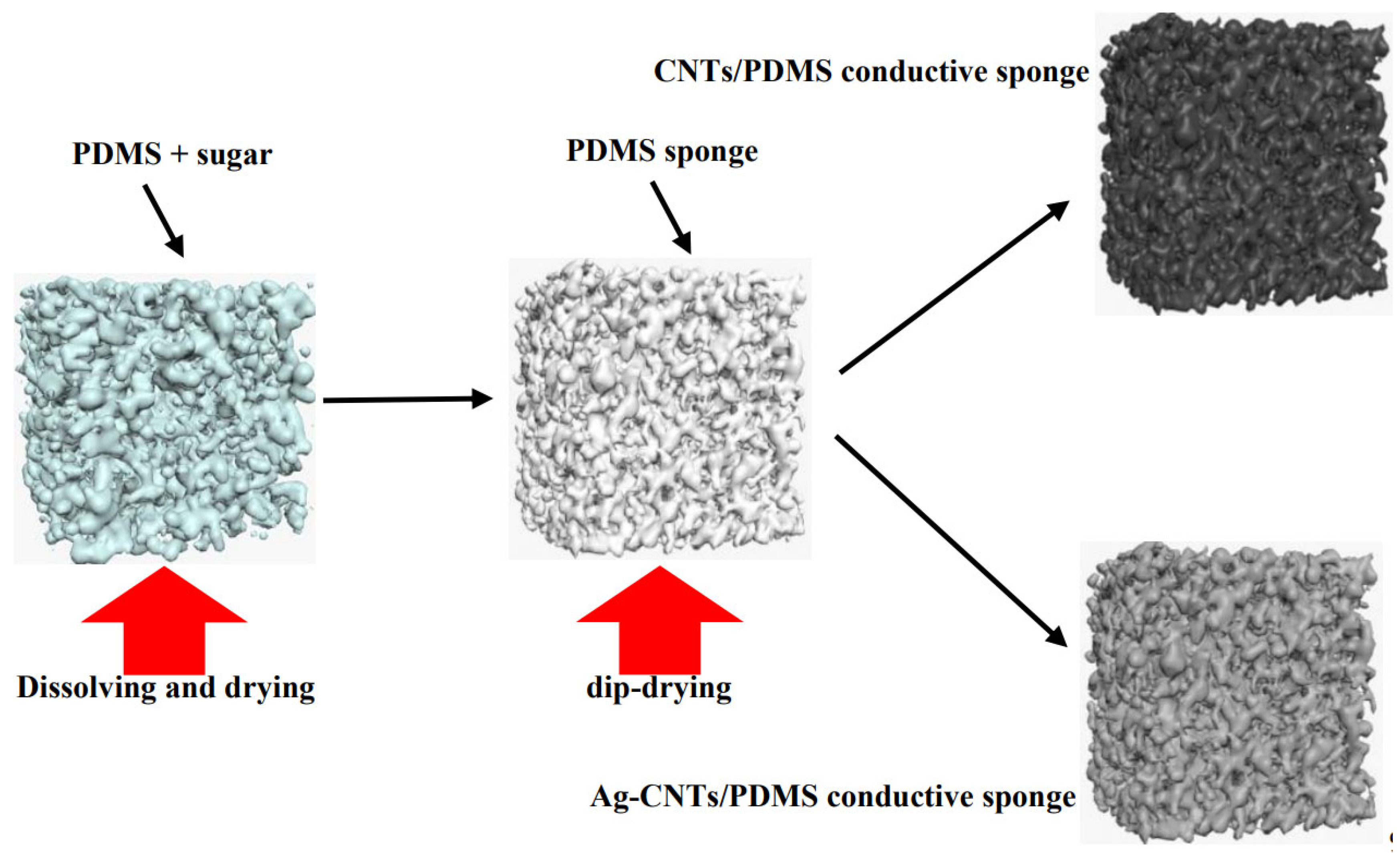
Figure 2.
The SEM images of the CNTs/PDMS conductive sponge (a) 90 multiples (b) 50000 multiples. The SEM images of the Ag-CNTs/PDMS conductive sponge (c) 100 multiples (d) 100000 multiples. The SEM images of the Ag-CNTs/PDMS particles (e) 20000 multiples (f) 150000 multiples.
Figure 2.
The SEM images of the CNTs/PDMS conductive sponge (a) 90 multiples (b) 50000 multiples. The SEM images of the Ag-CNTs/PDMS conductive sponge (c) 100 multiples (d) 100000 multiples. The SEM images of the Ag-CNTs/PDMS particles (e) 20000 multiples (f) 150000 multiples.
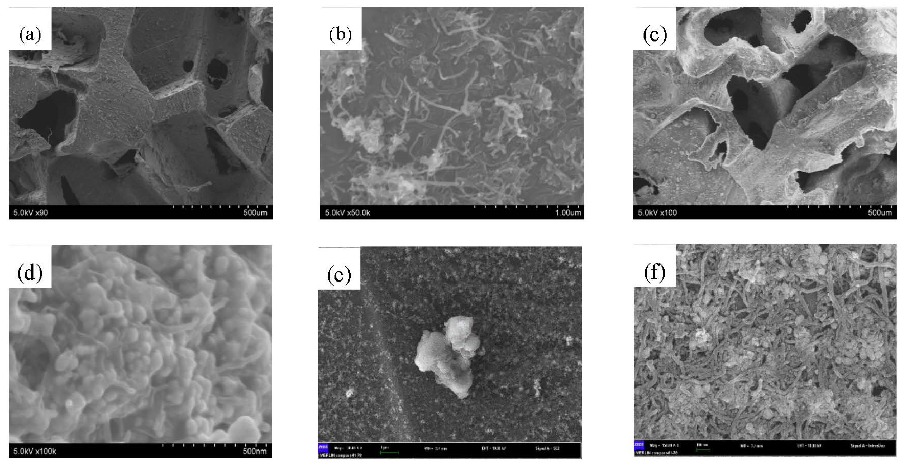
Figure 3.
Schematic diagram of the compression contact point of conductive path (a) Initial state (b) Compression state.
Figure 3.
Schematic diagram of the compression contact point of conductive path (a) Initial state (b) Compression state.
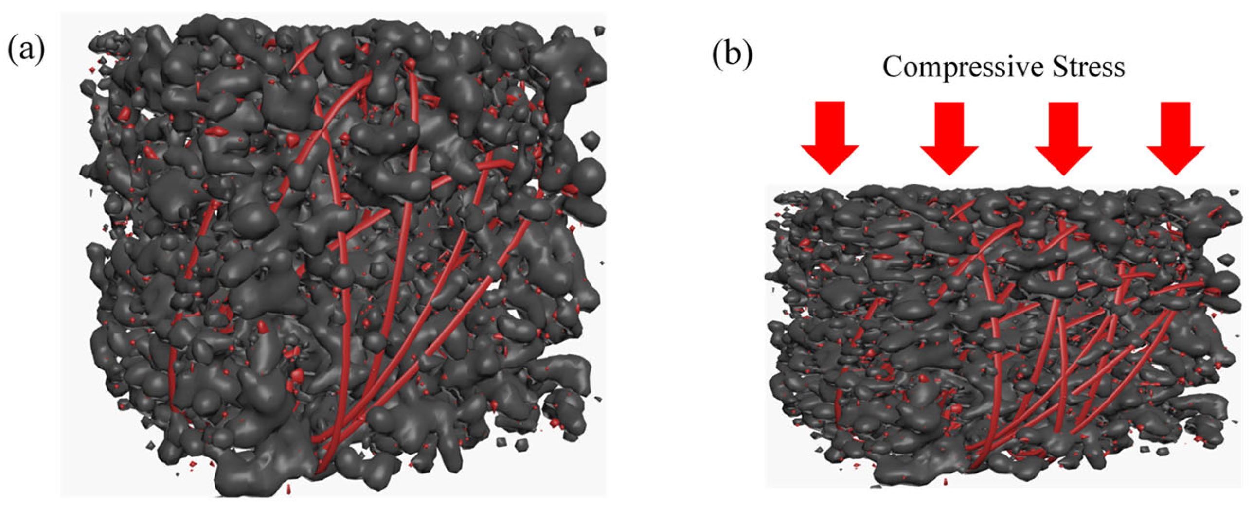
Figure 4.
Resistance change rate-pressure curve of CNTs/PDMS (heat-drying) flexible pressure sensor (a) Weight ratio of 0.5 wt%~2.5 wt% (b) Weight ratio of 2.5 wt%~5.0 wt%. Sensitivity fitting curves of flexible pressure sensor (c) Weight ratio of 0.5 wt% (d) Weight ratio of 1.0 wt% (e) Weight ratio of 1.5 wt% (f) Weight ratio of 2.0 wt% (g) Weight ratio of 2.5 wt% (h) Weight ratio of 3.5 wt% (i) Weight ratio of 5.0 wt%.
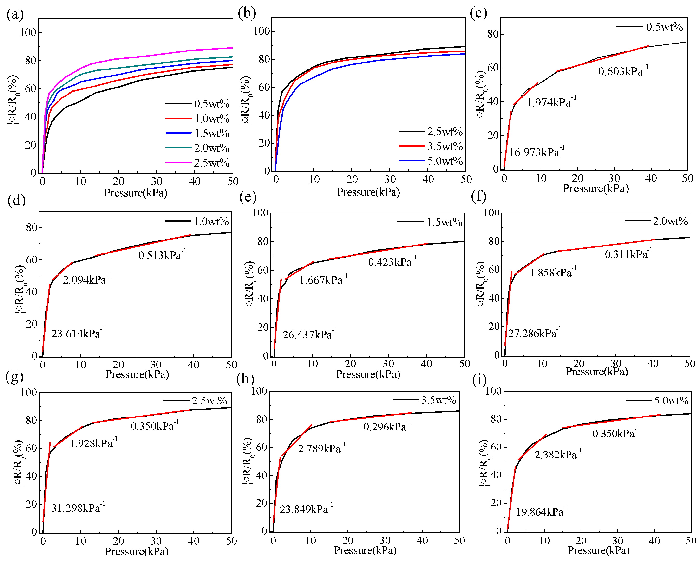
Figure 5.
Resistance change rate-pressure curve of CNTs/PDMS (freeze-drying) flexible pressure sensor (a) Weight ratio of 0.5 wt%~3.5 wt% (b) Weight ratio of 3.5 wt%~5.0 wt%. Sensitivity fitting curves of flexible pressure sensor (c) Weight ratio of 0.5 wt% (d) Weight ratio of 1.0 wt% (e) Weight ratio of 1.5 wt% (f) Weight ratio of 2.0 wt% (g) Weight ratio of 2.5 wt% (h) Weight ratio of 3.5 wt% (i) Weight ratio of 5.0 wt%.
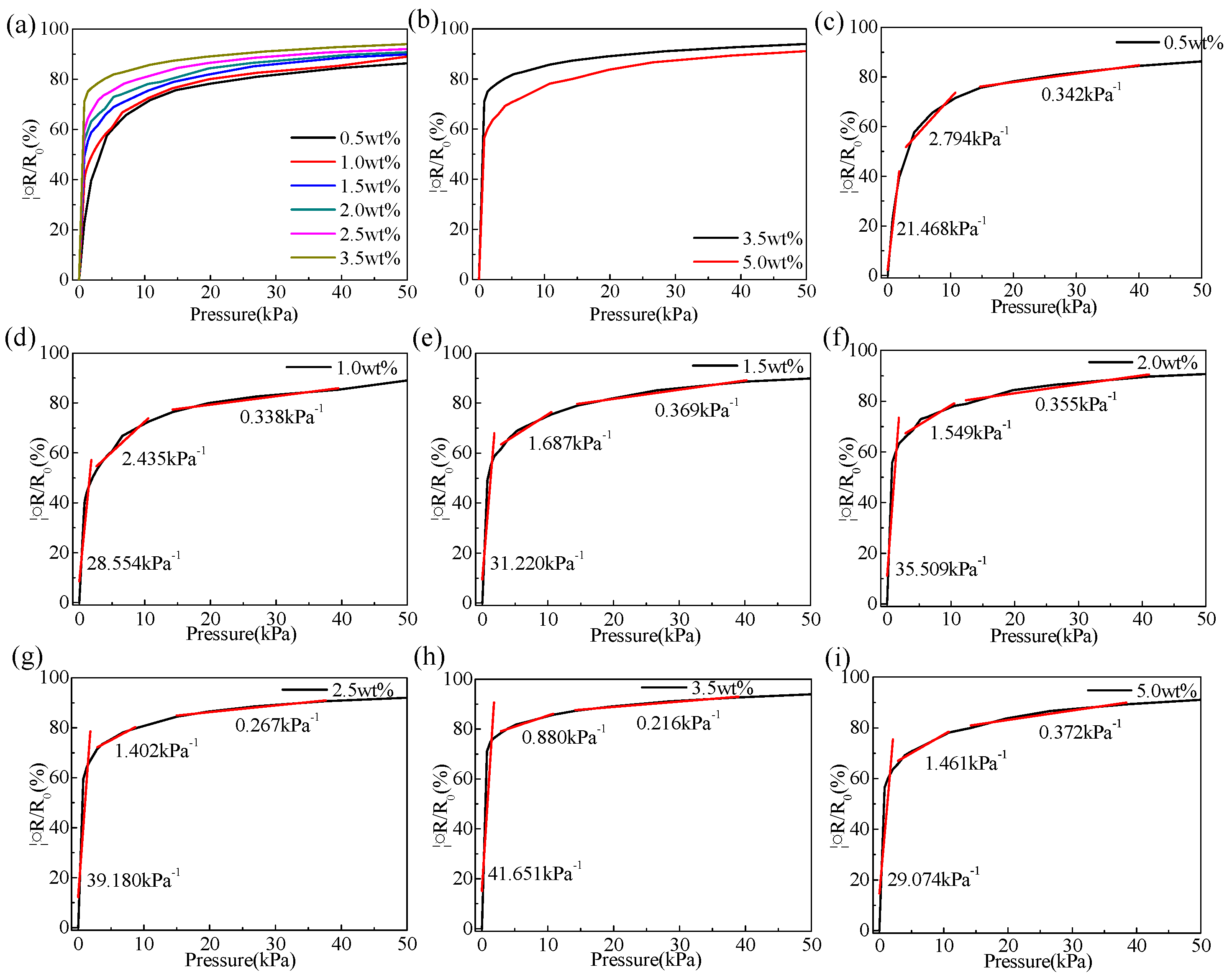
Figure 6.
(a) Resistance change rate-pressure curve of Ag-CNTs/PDMS flexible pressure sensor with weight ratio of 0.5 wt%~5.0 wt%. Sensitivity fitting curves of flexible pressure sensor (b) Weight ratio of 0.5 wt% (c) Weight ratio of 1.0 wt% (d) Weight ratio of 1.5 wt% (e) Weight ratio of 2.0 wt% (f) Weight ratio of 2.5 wt% g) Weight ratio of 3.5 wt% (h) Weight ratio of 5.0 wt%. Sensitivity curves of flexible pressure sensor.
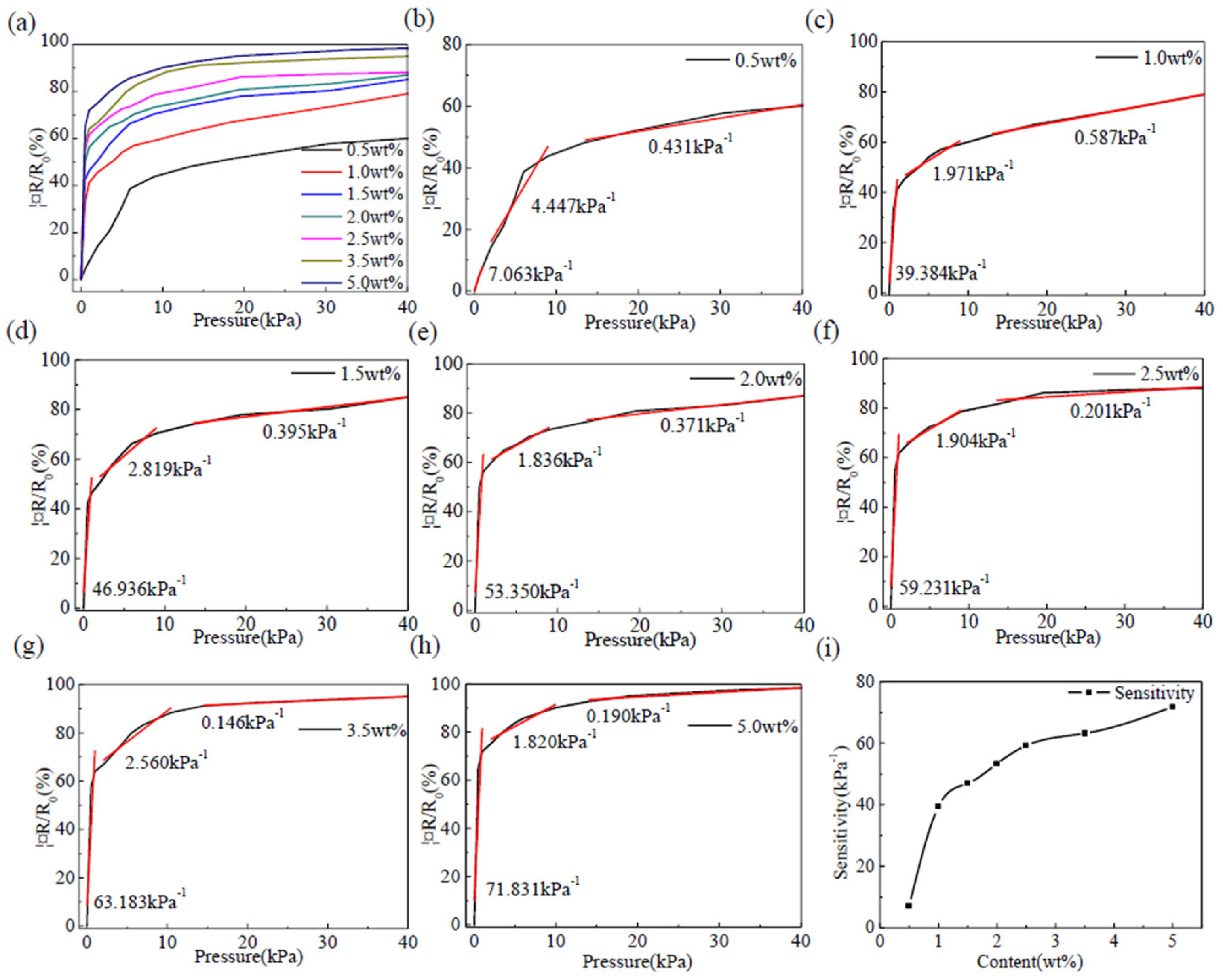
Figure 7.
(a) Comparison of sensitivity of three different flexible pressure sensors. (b) Pressure Stability Test of Flexible Pressure Sensor. (c) Strain Stability Test of Flexible Pressure Sensor. Hysteresis test curve of Ag-CNTs/PDMS flexible pressure sensor (d) Weight ratio of 2.5 wt% (e) Weight ratio of 3.5 wt% (f) Weight ratio of 5.0 wt%.
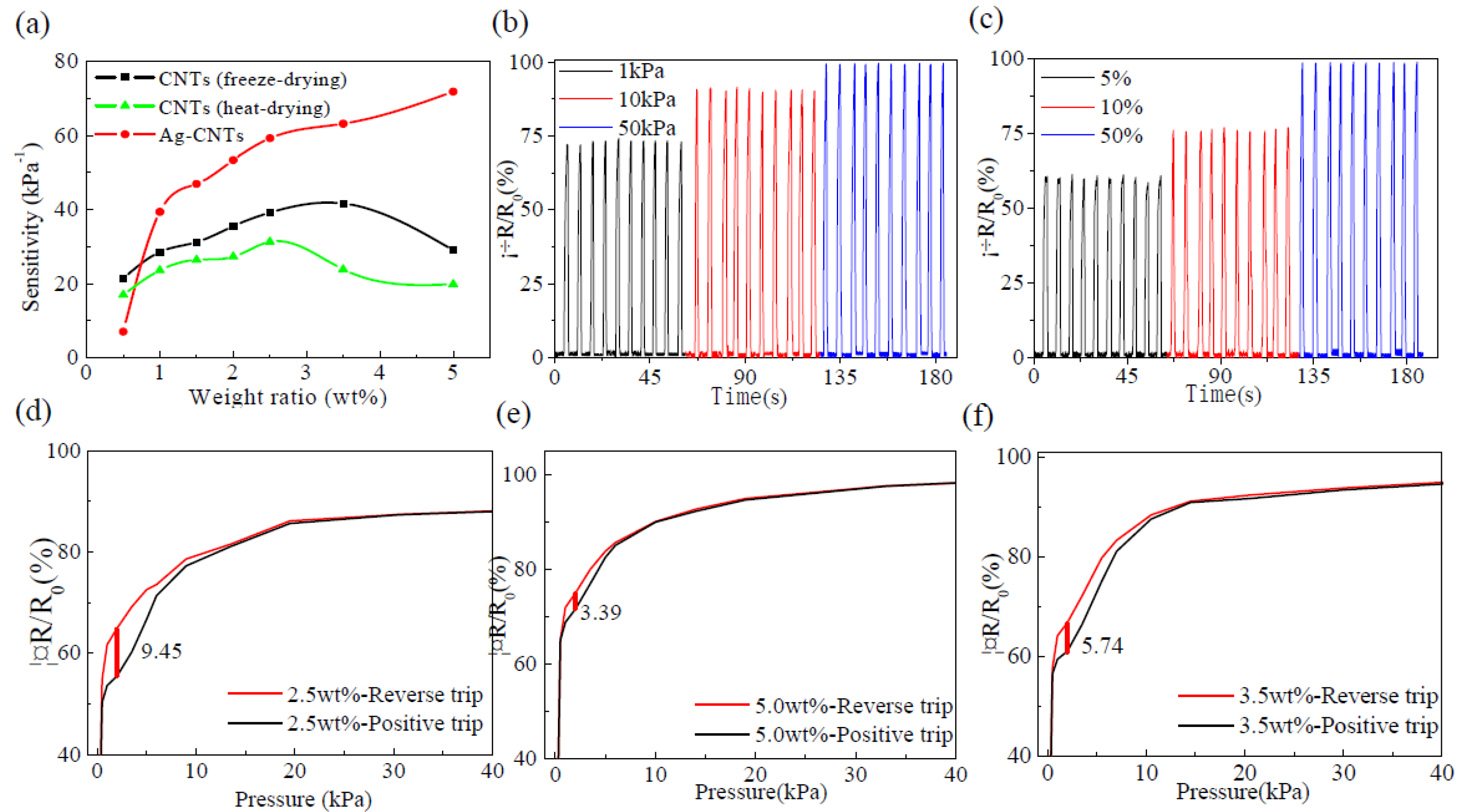
Figure 8.
(a) Resistance stability experiments at different temperatures. (b) I-V characteristic curve of the sensor (at room temperature). Temperature-resistance curve of sensor with different contents (c) Weight ratio of 2.5 wt% (d) Weight ratio of 3.5 wt% (e) Weight ratio of 5.0 wt%. The coupled test curve under four kinds of pressure (f) 4 kPa (g) 8 kPa (h) 20 kPa (i) 40 kPa.
Disclaimer/Publisher’s Note: The statements, opinions and data contained in all publications are solely those of the individual author(s) and contributor(s) and not of MDPI and/or the editor(s). MDPI and/or the editor(s) disclaim responsibility for any injury to people or property resulting from any ideas, methods, instructions or products referred to in the content. |
© 2024 by the authors. Licensee MDPI, Basel, Switzerland. This article is an open access article distributed under the terms and conditions of the Creative Commons Attribution (CC BY) license (http://creativecommons.org/licenses/by/4.0/).
Copyright: This open access article is published under a Creative Commons CC BY 4.0 license, which permit the free download, distribution, and reuse, provided that the author and preprint are cited in any reuse.


