
Submitted:
11 July 2024
Posted:
12 July 2024
You are already at the latest version
Abstract
For the first time, mathematical models were obtained for evaluating biomedical images using fuzzy set methods on the basis of expert knowledge bases, which made it possible to carry out complex qualitative diagnostics and increase the reliability and efficiency of diagnosis, to form a methodology for analyzing biomedical images based on the fuzzy set apparatus, which allowed to more fully assess the level of the disease for glaucoma. Aspects of practical implementation of the optical-electronic system of biomedical information processing are considered. An algorithm and an optical-electronic system of biomedical image analysis are proposed, which are used to increase the informativeness and reliability of diagnosing eye pathologies, in particular, glaucoma.
Keywords:
optical and electronic expert system
; diagnosing eye pathology
; glaucoma
1. Introduction
When experts form a reference sample of images of the fundus, conflicting moments may arise due to the ambiguity of the images. Practice has shown that even one expert at different times (after a week, a month) can differently assess whether the same image belongs to glaucoma or not. It is natural that different experts often have different opinions about the attribution of fundus images to glaucoma. Therefore, when forming the knowledge base of the expert system, it is necessary to provide procedures for assessing the convergence and reproducibility of the results of creating a reference sample [1,2,3]. The result of the work of the optical-electronic expert system is a conclusion about the presence of glaucoma up to a certain type with an indication of the probability assessment. The latter will require the creation of the necessary volume of a representative reference sample of images [4,5,6]. A feature of the considered expert system is that, along with the knowledge of experts accumulated in it, a database is created based on the results of measuring quantitative features obtained as a result of automated image processing. Next, a conclusion is formed based on the assessment of the probability of the considered image belonging to the list of possible types of glaucoma [2,7,8,9]. Since the conclusion based on the results of drug research using an expert system is formed on the basis of the results of computer image processing, it is necessary to consider the factors affecting the accuracy of the measurements performed in the system [10, 12,13]. For the considered task of automating the analysis of the fundus, at the first stage, image improvement procedures are performed, which are associated with the suppression of image-distorting factors (filtering of obstacles, elimination of lighting irregularities, etc.). At the description stage, the features characteristic of the object are calculated, on the basis of which, at the third stage, the object is assigned to one or another class. The key of these three stages is the description stage. The recognition result depends on the choice of features and their informativeness (the ability to attribute the object to one or another class based on the value of the feature). We can distinguish two groups of factors that influence the recognition result: the first is the properties of the object itself (images of the fundus are very diverse); the second is the image formation conditions (sensor noise, uneven illumination of the object, etc.) [14,15]. The purpose of this work is to develop a conceptual model of an optical-electronic expert system for the diagnosis of glaucoma using computer processing methods, as well as to analyze the influence of factors influencing the result of fundus image recognition [16,17,18].
2. Method
The proposed approach to the recognition of images of the fundus is based on the use of the knowledge of specialists in the field of ophthalmology and consists in creating an expert system for the diagnosis of glaucoma. The basis of the system is a reference sample of digital images, the description of which is stored in the knowledge base, an important component of the system is the analytical subsystem, which includes many rules by which decisions are made (Figure 1) [19,20,21]. Factors that have a dominant influence on the correctness of image recognition. As a result of the conducted research, a number of factors that have the most significant impact on the accuracy of the measurement results were identified, and they can be divided into three groups based on the type of source (Figure 2). For the considered system, instrumental factors can be classified into two groups: the first - factors due to physical processes in the used equipment; the second - factors due to the influence of external conditions. The first group of instrumental factors includes the noise of the image sensor, color distortions of the camera, brightness distortions, diffraction effects of the optical system, uneven spectral characteristics of the illuminator in the ophthalmoscope, uneven illumination of the drug in the field of view of the camera, etc. The factors of the second group include factors determined by the external conditions of system application [22,23,24].
So, for example, the image registered in the system can be affected by such factors as the presence of bright external lighting (sunlight), as a result of which the contrast of the image can decrease. In addition, external factors include surface vibration (this can lead to image distortion at large exposures) [25,26]. First of all, methodical factors include the measurement model and mathematical methods of image processing, which are implemented in the system software, discretization and quantization operations when forming a digital image. A group of factors depending on the user is related to the setting of the ophthalmoscope (choice of the lens, position of the condenser, field and aperture diaphragm, voltage of the lamp and light flux correction filters, position of the lens focus). Along with this, this group includes factors related to the selection of the field for research and positioning of the research object in the field of view of the camera, and factors that depend on the user in the interactive mode of image processing (when the processing parameters are specified by the user during the application software implementing image processing)[27-29]. A conceptual model of an expert system for diagnosing glaucoma is proposed, which will reduce the ambiguity of the interpretation of research objects. Factors affecting the correctness of recognition of complex objects (images of the fundus) using an expert system based on methods of computer ophthalmoscopy were considered (Table 1).
To diagnose glaucoma, we take into account the following indicators
X1 - Intraocular pressure, mm .
X2 - Field of vision
X3 - The ratio of the diameter of the excavation to the diameter of the DZN
X4 - The ratio of the excavation area to the area of DZN
X5 - The ratio of the volume of excavation to the volume of DZN
X6 - Excavation area
X7 - Excavation volume
X8 - Neuroretinal strip area
X9 - Volume of the neuroretinal strip
X10 - The average thickness of the layer of nerve fibers along the edge of the disc
X11 - Cross-sectional area of the layer of nerve fibers along the edge of the disc.
For variable
For variable
For variable
For variable
3. Software-Algorithmic Implementation for Processing Biomedical Images
During the analysis of the characteristics of the fundus, increase the reliability of the final assessment of fundus images by using expert methods. The proposed approach to the recognition of images of the fundus is based on the use of the knowledge of specialists in the field of ophthalmology and consists in creating an expert system for the diagnosis of glaucoma. The basis of the system is a reference sample of digital images, the description of which is stored in the knowledge base, an important component of the system is the analytical subsystem, which includes many rules by which decisions are made. To obtain a diagnosis with the help of an expert database, we suggest using elements of fuzzy logic. We will build the model on the basis of actual data. (Table 1). Using the algorithm of the processing method based on the fuzzy logic apparatus, we get:
Figure 3.
Initial data input request.
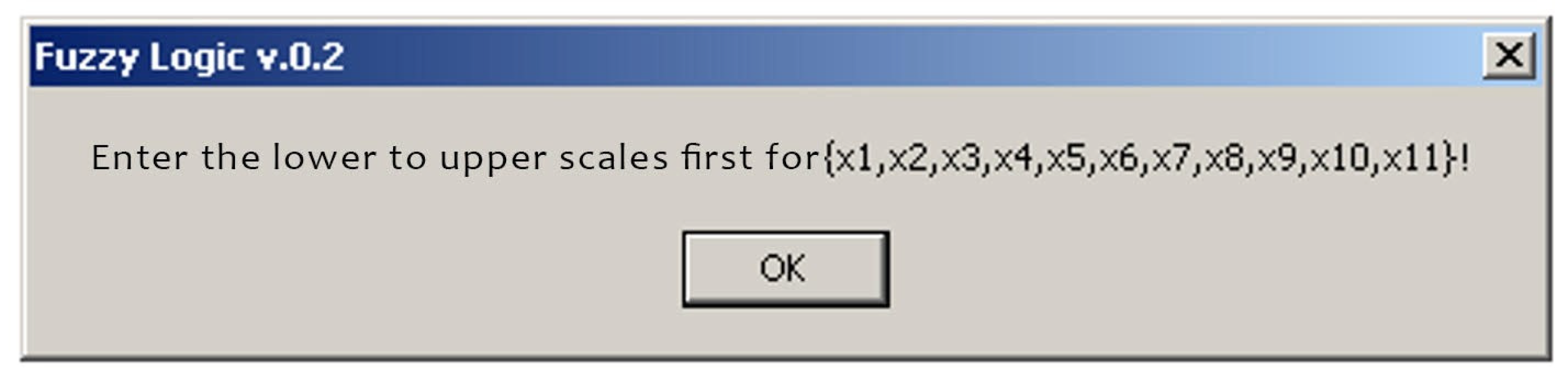
Figure 4.
Input of initial data.
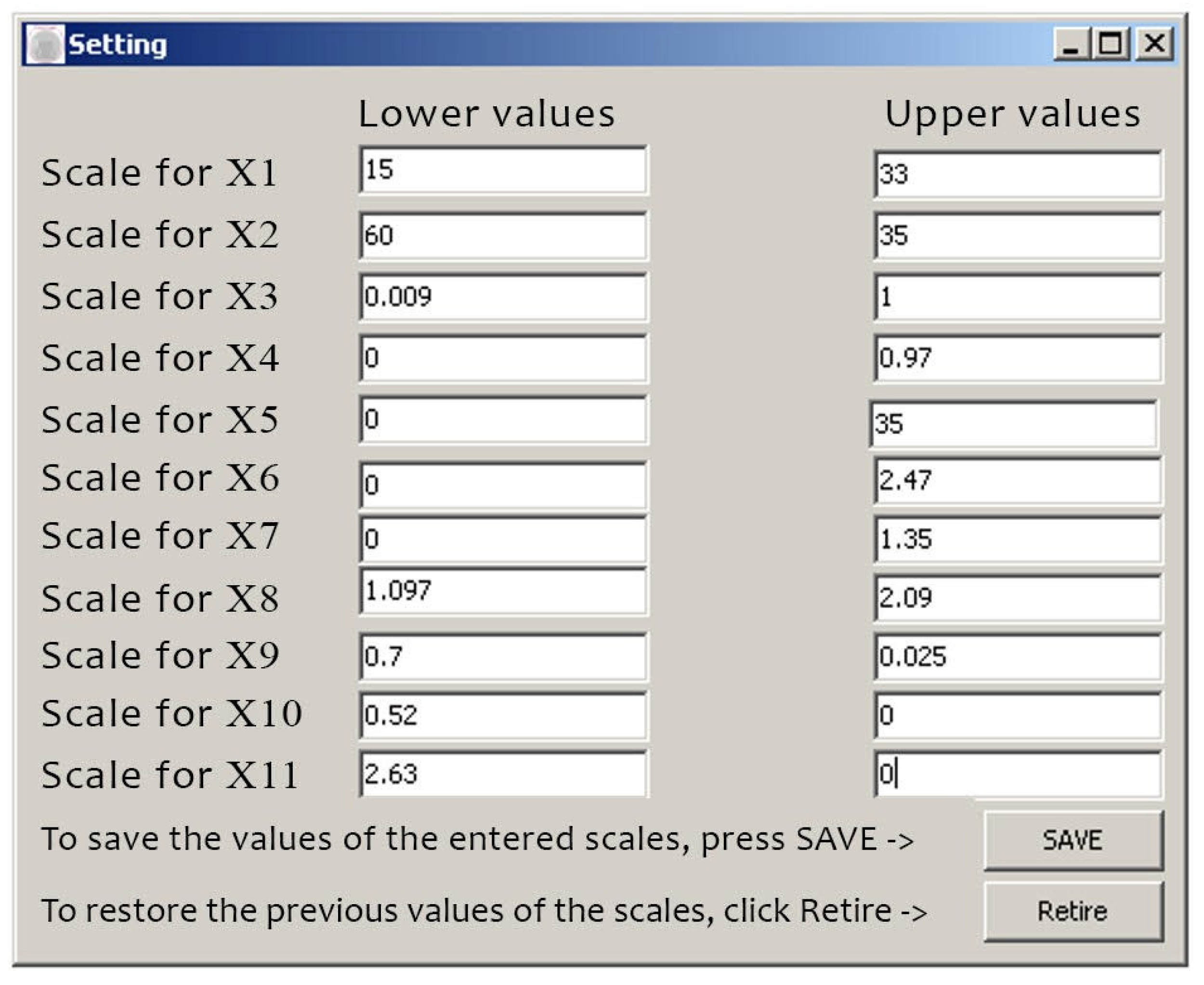
When saving the data, i.e. entering the lower and upper values, we can enter the patient’s data:
Figure 5.
Entering the patient’s input data .
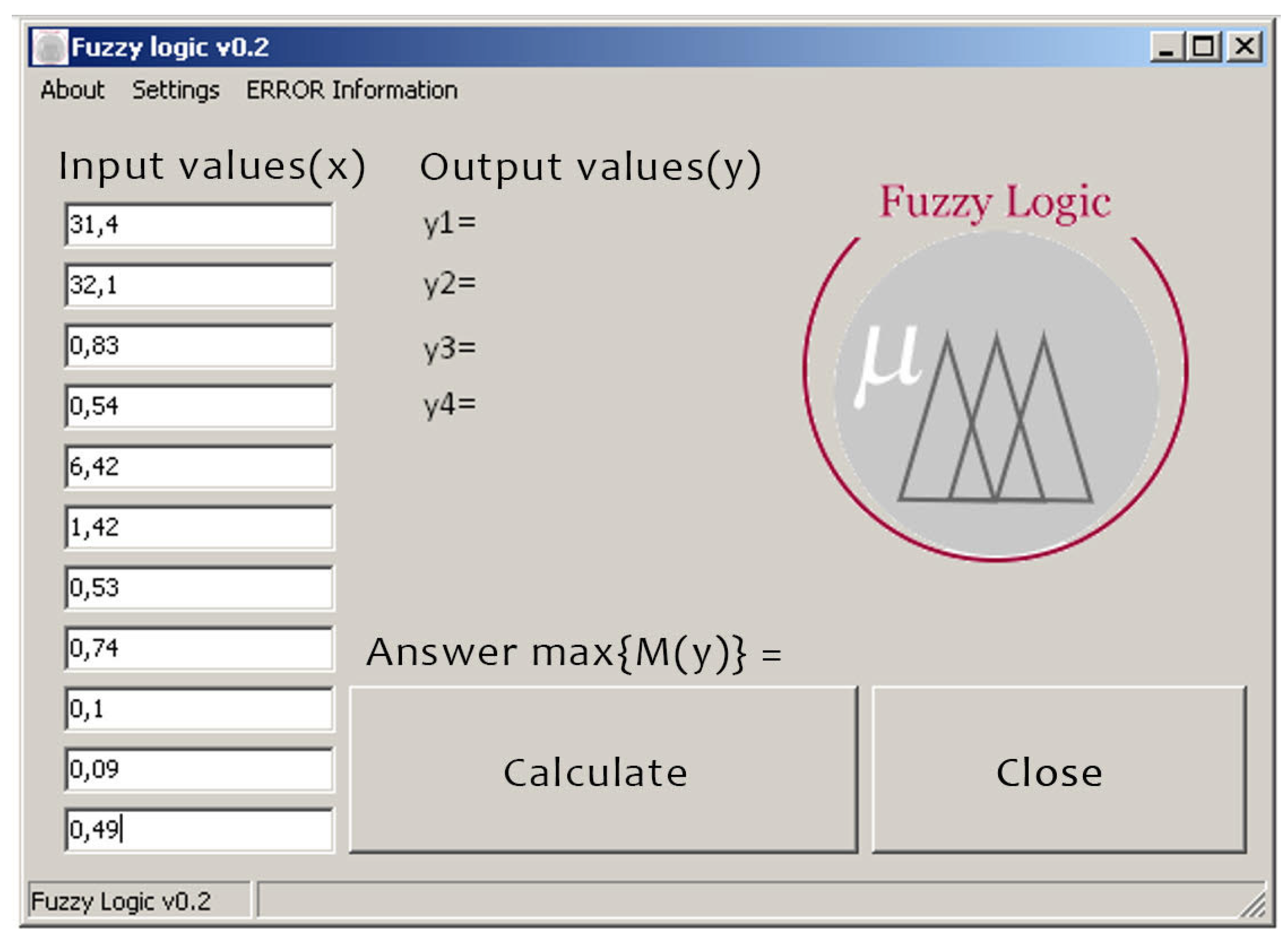
Having obtained the result, we can conclude that the patient has glaucoma of the 3rd degree.
4. Physical Modeling of the Optical-Electronic System for Researching Pathologies of the Fundus
The optical-electronic system for obtaining an image of the retina of the eye refers to medicine, namely to devices for examining the fundus, and can be used in ophthalmology to conduct medical and biological research, namely: to fix the image of the retina. At the same time, the optical channel is realized as follows. The radiation flow coming from the radiating surface of the source to the remote illuminating surface (1):
where L is the brightness of the emitting surface;
S source – the area of the radiating surface;
S sq. is the area of the illuminating surface;
is the angle between the direction of radiation propagation and the normal to the radiating surface;
id s the angle between the direction of radiation propagation and the normal to the illuminating surface;
l is the distance between the surfaces.
If the lighting system directs radiation into the eye through a pupil area with an area Ssource, then this area can be considered as a light-emitting surface, the brightness of which Llaser due to the transition of light rays from the air to the eye is related to the brightness of the source - the LED Ldiode by the expression (1, 2) :
– is the average refractive index of eye tissues. Taking into account expression (2) and the transmission coefficient of the optical system of the eye , expression (1) for the light flux falling on the retina will be written in the form:
where is the area of the retina; leye is the distance between the pupil and the retina.
When the light flux spreads along the optical axis of the eye, which is assumed to be perpendicular to the planes of the pupil and retina , the illumination of the retina will be:
Expression (4) is true for the illumination of a retinal point lying on the optical axis of the eye. However, since the fundus is a sphere and due to the multiple reflection of light rays inside the eye, it can be assumed that the illumination of the entire retina is uniform and is determined by expression (4). A uniformly illuminated retina, diffusely reflecting the light stream falling on it, represents a secondary light source, the brightness of which will be equal to:
where is the diffusion reflection coefficient.
Illumination of the retinal image on the photomatrix, which is built by the optical system:
where is the transmission coefficient of the optical system;
is the refractive index of the medium in the image space ;
n is the index of refraction of the medium in the space of objects (n = noka);
D is the diameter of the entrance pupil of the optical system;
is the focal length of the optical system;
– linear increase of the optical system in the pupils;
is the linear increase of the optical system.
Substituting (5) into (6) and assuming a linear increase in the pupils , for the illumination of the retinal image on the photo matrix we obtain:
Let’s assume that = 0,5; = 0,9; = 0,2; = 24 diameter = 24 mm. The maximum brightness of the light source that can be transmitted when directly observed is 7500 . For so that the patient does not feel discomfort, as an illuminator we choose an LED for which . Let’s also assume that the projection of the source onto the pupil of the eye occupies 50% of its area. In this case, with a pupil diameter of 6 mm, Sd.pup = 14.13 mm. To perceive the image, we will use the 6.6 Megapixel CMOS photo matrix NOII4SM6600A, the main indicators of which are as follows:

Table 2.
Formation of an expert base in the diagnosis of glaucoma.
| Dimensional capacity | 2210 × 3002 |
|---|---|
| Optical format, inch | 1 |
| Range of spectral sensitivity, | 400...1000 |
| Apparent sensitivity, | 2.01 |
| Dark signal, | 3.37 |
1 Tables may have a footer.
The required linear increase of the optical system can be determined by the ratio that corresponds to the condition under which the retinal image occupies the largest part of the photomatrix area:
where is the height of the photomatrix;
Dretina is the diameter of the retina.
The optical matrix format of 1 inch corresponds to the size of 12.8 × 9.6 mm. The diameter of the human retina is 22 mm. Then
By substituting numerical values for the definition in expression (7), we get:
To carry out further calculations, we will determine the illumination of the photomatrix , at which the value of the useful output signal will be comparable to the dark one. The minimum illumination of the image, at which it is indistinguishable from the background noise, is found using the sensitivity of the photomatrix and the value of the dark signal:
To obtain a good image of the retina, the illumination of the photo matrix must be at least 10 times higher than this value, therefore:
Then, from expression (9) for the geometric luminous intensity of the optical system, we have: In order to use the entire field of the optical system, its entrance pupil must be aligned with the plane of the eye pupil. In this case, the field aperture will be the frame of the photomatrix, and with the linear magnification selected in accordance with expression (8), the image of the entire retina will be formed on the photomatrix. The diameter of the entrance pupil of the optical system D is chosen equal to 3 mm. As a result, the area of the entrance pupil of the optical system will be equal to 7.065 , which is 25% of the area of the pupil of the eye with a pupil diameter of 6 mm. Then, from expression (10) for the focal length of the optical system, we obtain:
When calculating the focal length of the optical system, its linear increase in the pupils was taken to be equal to 1. This corresponds to the case when the distance from the front focus of the optical system to the input pupil is equal to the front focal length of the optical system:
(mm)
The distance from the front focus to the retina will be equal to:
(mm) The distance from the back focus to the retinal image formed in the photomatrix plane is determined using the linear magnification of the optical system :
5. Evaluation of Metrological Indicators
For most medical and biological studies, the degree of probability of an error-free forecast equal to 95% is considered sufficient, and the number of cases of the general population in which deviations from the patterns established during a sample study may be observed will not exceed 5%. In a number of studies related, for example, to the use of highly toxic substances, vaccines, surgical treatment, etc., as a result of which serious diseases, complications, and fatal consequences are possible, the degree of probability P = 99.7% is used, i.e. no more than in 1% of cases of the general population, deviations from the regularities established in the sample population are possible. The given degree of probability (P) of an error-free forecast corresponds to a certain, substituted into the formula, value of the criterion t, which also depends on the number of observations. When n > 30, the degree of probability of an error-free forecast P = 99.7% corresponds to the value of t = 3, and when P = 95.5% - the value of . When n < 30, the value of t at the appropriate degree of probability of an error-free forecast is determined according to a special table (N.A. Plokhinsky). We will determine the error of representativeness (mp) and confidence limits of the relative indicator of the general population () in relation to the table of results obtained by the diagnosis of an ophthalmologist and with the help of an expert database. A group of glaucoma patients consisting of 42 people aged 50-65 years, but with different stages, was taken.
Table 2 - Comparison of the received diagnoses by different methods
Table 3.
Formation of an expert base in the diagnosis of glaucoma.
| Dimensional capacity | Stages of glaucoma | Number of patients in percent | Number of patients | Stages of glaucoma | Number of patients in percent |
|---|---|---|---|---|---|
| 18 | I | 43 | 17 | I | 40 |
| 6 | II | 14 | 5 | II | 12 |
| 18 | III | 43 | 20 | III | 48 |
1 Tables may have a footer.
Determination of the representativeness error of the relative indicator according to the diagnosis of the ophthalmologist:
Determination of the error of representativeness of the relative indicator according to the diagnosis obtained with the help of the expert database:
The confidence limits of the average value of the general population () are calculated as follows:
- it is necessary to set the degree of probability of an error-free forecast ();
- at a given degree of probability and the number of observations is more than 30, the value of the criterion t is equal to 2 (t = 2). Then
Then
Then
Then
Then
Then
Taking into account the results of the calculation of the confidence limits of the average value of the general population (), we can establish with the probability of an error-free forecast P = 95% that the frequency of detection of stage I glaucoma at the age of 50-65 will be in the range from 27.72 % to 58, 28 % of cases (diagnosis by an ophthalmologist) and from 24.88 % to 55.12 % (diagnosis obtained using an expert database). The frequency of detection of stage II glaucoma at the age of 50-65 years will range from 3.30 % to 24.70 % of cases (diagnosis by an ophthalmologist) and from 1.98 % to 22.02 % (diagnosis obtained by expert base). The frequency of detection of stage III glaucoma at the age of 50-65 years will range from 27.72 % to 58.28 % of cases (diagnosis by an ophthalmologist) and from 32.58 % to 63.42 % (diagnosis obtained by expert base).
6. Recommendations for the Implementation of the Optic-Electronic System for Obtaining an Image of the Retina of the Eye
In Figure 6 shows a schematic representation of the path of the rays in the design of the photographic ophthalmoscope, which is designed to fix the image of the retina, in Figure 7 presents an optical-electronic system for the analysis of ophthalmological images, in Figure 8 – the image of the retina of the human eye, which was obtained as a result of using a photographic ophthalmoscope, is presented.
Photographic ophthalmoscope, the body of the optical nozzle 4, in which the optical system containing the diaphragm 7, the first 8, the second 10 mirrors and the condenser 9 is located. In addition, the device contains a digital camera 5, a white LED 6, a digital camera lens 11, a matrix digital camera 12, as well as in Figure 6 shows the location of the patient’s eye 1, its pupil 2 and its lens 3, and the patient’s eye 1, which has a pupil 2 and a lens 3, is connected to the output of the second mirror 10, the input of which is connected to the input of the condenser 9 and the lens of the digital camera 11, the output of which is connected to the input of the matrix of the digital camera 12, the output of the condenser 9 is connected to the first mirror 8, the input of which is connected to the diaphragm 7, which is connected to the output of the white LED 6 [30-32]. The photographic ophthalmoscope works as follows. Scattered light from the white LED 6, through the aperture 7 is focused by the system of mirrors 8, 10 and the condenser 9, passing through the pupil 2 and the lens 3 of the eye 1, illuminates the fundus. The optical system, which consists of the diaphragm 7, mirrors 8 and 10 and the condenser 9, is placed in the body of the optical nozzle 4. The image of the fundus passes through the optical system of the eye 1 and in a parallel beam hits the lens of the digital camera 11 contained in the digital camera 5, where an enlarged image of the retina is formed (Figure 4.4), which is displayed using a digital matrix 12 for further analysis by a doctor. Due to the introduction of a white LED, mirrors, condenser, lens and matrix of a digital camera, the functionality of the ophthalmoscope was increased, which gives the doctor the opportunity to improve the diagnosis of eye diseases and to be able to reproduce the medical history.
7. Conclusions
For the first time, mathematical models were obtained for evaluating biomedical images using fuzzy set methods on the basis of expert knowledge bases, which made it possible to carry out complex qualitative diagnostics and increase the reliability and efficiency of diagnosis, to form a methodology for analyzing biomedical images based on the fuzzy set apparatus, which allowed to more fully assess the level of the disease for glaucoma. Aspects of practical implementation of the optical-electronic system of biomedical information processing are considered. An algorithm and an optical-electronic system of biomedical image analysis are proposed, which are used to increase the informativeness and reliability of diagnosing eye pathologies, in particular, glaucoma. On the basis of the developed model and algorithms, a hardware and software implementation was created, experimental and medical studies of the obtained system indicators were conducted. Examples of practical application of the developed optical-electronic system for the analysis of eye pathologies are given. The main practical result is that the expediency and reliability of such an optical-electronic system has been practically confirmed.
Acknowledgments
This research has been funded by the Committee of Science of the Ministry of Science and Higher Education of the Republic of Kazakhstan (Grant No. AP 19675574).
Conflicts of Interest
The authors declare no conflicts of interest.
References
- Sebestyen, G.S. Decision Making Processes in Pattern Recognition. N.Y.: Macmillan 1995, 10, 237. [Google Scholar]
- Fukushima, K. Neural Network for Visual Pattern Recognition. In Comput; 1988, 21, 65–116. [Google Scholar] [CrossRef]
- Dogru, M. ; Katakami, Ch, Inoue, M. Ocular microcirculation changes in noninsulin-dependent diabetes mellitus. Ophthalmology, 2001; V. 108. - № 3. 586–592. [Google Scholar]
- Novotny, H.; Alvis, D. A method of photographing fluorescence in circulating blood in the human retina. Circulation, 1961; V. 24. - № 7. 82–86. [Google Scholar]
- Federman, J.; Brown, G.; Felberg, N.; Felton, S. Experimental ocular angiogenesisAmerican Journal of Ophtalmology 1980, 10, 231–237.
- Balashevich, I.; Izmailov, A.; Levochkin, A. Diagnostic possibilities of digital fluorescein angiography Ophthalmosurgery 1998, 38–46.
- Crittin, M.; Schmidt, H.; Riva, E.C. Hemoglobin oxygen saturation in the human ocular fundus measured by reflectance oximetry: preliliminary data in retinal veins. Klin. Monatsbl Augenheilkd 2002, 1, 289–291. [Google Scholar] [CrossRef] [PubMed]
- Rotshtein, A. Design and Tuning of Fussy IF – THEN Vuly for Medical Didicol Diagnosis. In Fussy and Neuro-Fussy Systems in Medicine (Eds: N. Teodovescu, A. Kandel, I. Lain.). USA. CRC-Press 1998, 1, 235–295. [Google Scholar]
- Bardenheier, B.H.; Lin, J.; Zhuo, X. , et al., Centers for Disease Control and Prevention. National Diabetes Statistics Report Accessed 2022. [Google Scholar]
- Murchison, A.P.; Hark, L.; Pizzi, L.T. , et al., Non-adherence to eye care in people with diabetes. BMJ Open Diabetes Res Care, 2017; 5, 235–295. [Google Scholar]
- Vuytsyk, V.; Gotra, O.Z.; Grigoryev, V.V. Expert systems: a training manual. Lviv, Ukraine: Liga-Press, 2006. [Google Scholar]
- Zavhorodnia, N.G.; Sarzhevska, L.E.; Ivakhnenko, O.M. “Eye changes in general diseases of the body: education - method. manual for intern doctors in the specialty "Ophthalmology", Zaporizhzhia, 2020, 83. [Google Scholar]
- Brownlee, J. “Machine Learning Mastery with Python: Understand Your Data, Create Accurate Models and Work Projects End-to-End,” 2nd Edition, California: Machine Learning Mastery (2019).
- Lu, W. et al. Application of computer-aided diagnosis in diabetic retinopathy screening: A review. Computers in Biology and Medicine 2018, 103, 337–349. [Google Scholar]
- Ting, D.; et al. Deep learning in ophthalmology: The technical and clinical considerations. Progress in Retinal and Eye Research 2019, 72, 100759. [Google Scholar] [CrossRef] [PubMed]
- Abràmoff, M.D.; et al. Automated analysis of retinal images for detection of referable diabetic retinopathy. JAMA Ophthalmology 2013, 131, 351–357. [Google Scholar] [CrossRef] [PubMed]
- Roychowdhury, S.; et al. , Automatic detection of diabetic retinopathy using deep learning International Conference on Computing, Analytics and Security Trends (CAST) 2017, 264–271.
- Bourne, R.R.A.; Stevens, G.A.; White, R.A. Causes of vision loss worldwide, 1990–2010: a systematic analysis. The Lancet Global Health 2013, 1, e339–e349. [Google Scholar] [CrossRef] [PubMed]
- Chakrabarti; Rahul; Harper, C.A.; Keeffe, J.E. Diabetic retinopathy management guidelines. Expert review of ophthalmology, 2012; 7.5, 417–439.
- Pavlov, S.V.; Karas, O.V.; Sholota, V.V. Processing and analysis of images in the multifunctional classification laser polarimetry system of biological objects. Proc. SPIE 2018, 10750. [Google Scholar]
- Pavlov, S.V.; Martianova, T.A.; Saldan, Y.R. Methods and computer tools for identifying diabetes-induced fundus pathology. Information Technology in Medical Diagnostics II. CRC Press, Balkema book, Taylor and Francis Group, London, UK, 87-99, 2019.
- Yosyp, S.; Pavlov, S.; Dina, V.; Wójcik, W. Efficiency of optical-electronic systems: methods application for the analysis of structural changes in the process of eye grounds diagnosis, Proc. SPIE 2017, 10445, Photonics Applications in Astronomy, Communications, Industry, and High Energy Physics Experiments.
- Lytvynenko, V.; Lurie, I.; Voronenko, M. The use of Bayesian methods in the task of localizing the narcotic substances distribution. International Scientific and Technical Conference on Computer Sciences and Information Technologies 2019, 2, 8929835. [Google Scholar]
- Friedman, Jerome, Trevor Hastie, and Robert Tibshirani., “The elements of statistical learning,” hastie.su. domains/ElemStatLearn (2009).
- Roman, K.; Yuriy, B.; Olga, S. Blur recognition using second fundamental form of image surface. Proc. SPIE 2015, 9816, Optical Fibers and Their Applications 2015, 98161A (17 December 2015).
- Avrunin, O.G.; Tymkovych, M.Y.; Saed, H.F.I. Application of 3D printing technologies in building patient-specific training systems for computing planning in rhinology. Information Technology in Medical Diagnostics II - Proceedings of the International Scientific Internet Conference on Computer Graphics and Image Processing and 48th International Scientific and Practical Conference on Application of Lasers in Medicine and Biology, 7 (2019).
- Mamyrbayev, O.; Pavlov, S.; Karas, O.; Saldan, I.; Momynzhanova, K.; Zhumagulova, S. Increasing the reliability of diagnosis of diabetic retinopathy based on machine learning. Eastern-European Journal of Enterprise Technologies 2024, 2, 17–26. [Google Scholar] [CrossRef]
- Abdiakhmetova, Z.M. Wavelet data processing in the problems of allocation in recovery well logging Journal of Theoretical and Applied Information Technology 15th March 2017. Vol.95. No 5.
- Baimakhan, R.; Kadirova, Z.; Seinassinova, A.; Baimakhan, A.; Mathematical, Z.A. Modeling of the Water Saturation Algorithm of the Mountain Slope on the Example of the Catastrophic Landslide of the Northern Tien Shan Ak Kain Mathematical Modelling of Engineering Problems 2021, 8, 467–476.
- Temirbekova, Z.; Pyrkova, A.; ZMAbdiakhmetova, Berdaly, A. Library of Fully Homomorphic Encryption on a Microcontroller SIST 2022 - 2022 International Conference on Smart Information Systems and Technologies, Proceedings, 2022. [CrossRef]
- Berdaly, A.; Temirbekova, Z.; Abdiakhmetova, Z.M. Comparative Machine-Learning Approach: Study for Heart Diseases SIST 2022 - 2022 International Conference on Smart Information Systems and Technologies, Proceedings, 2022. [CrossRef]
- Nussipova, F.; Rysbekov, S.; Abdiakhmetova, Z.; Kartbayev, A. Optimizing loss functions for improved energy demand prediction in smart power grids. International Journal of Electrical and Computer Engineering (IJECE) 2024, 14, 3415–3426. [Google Scholar] [CrossRef]
Figure 1.
Analytical subsystem, which includes many rules, according to which decision-making is carried out.
Figure 1.
Analytical subsystem, which includes many rules, according to which decision-making is carried out.
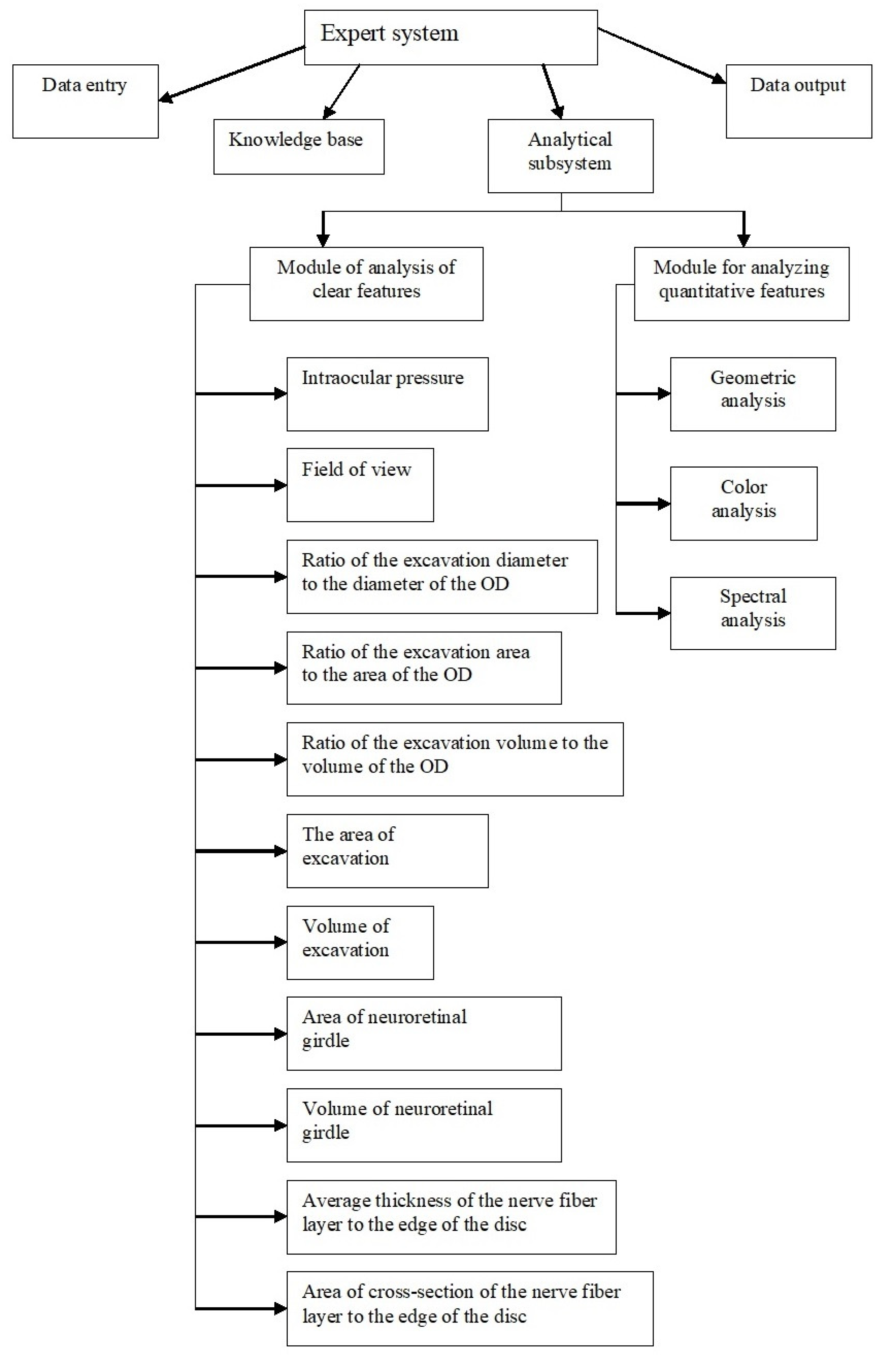
Figure 2.
Factors that have the most significant impact on the accuracy of measurement results.
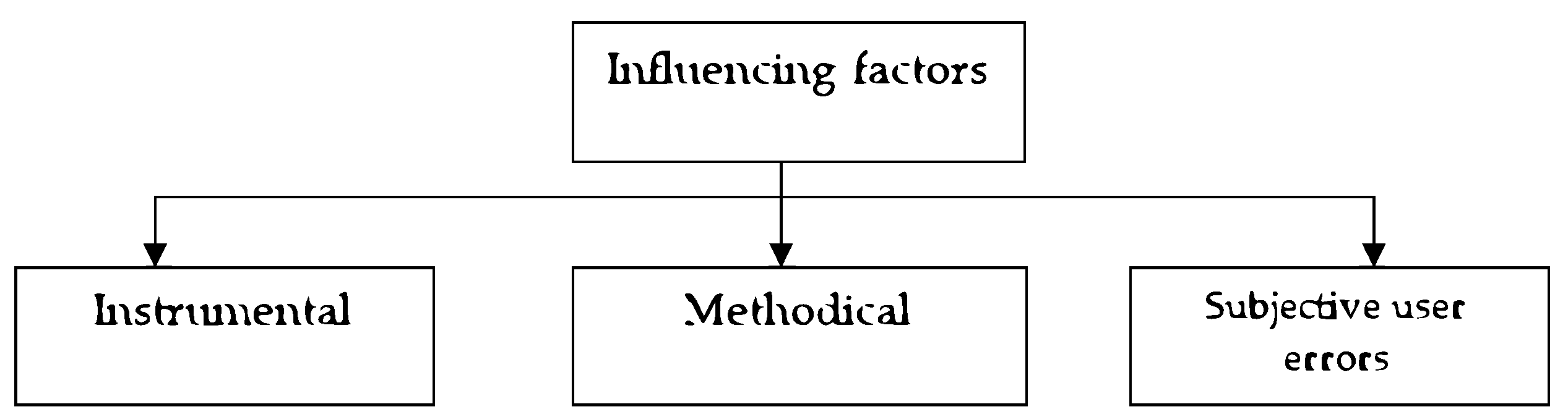
Figure 6.
This is a figure. Schemes follow the same formatting. If there are multiple panels, they should be listed as: (a) Description of what is contained in the first panel. (b) Description of what is contained in the second panel. Figures should be placed in the main text near to the first time they are cited. A caption on a single line should be centered.
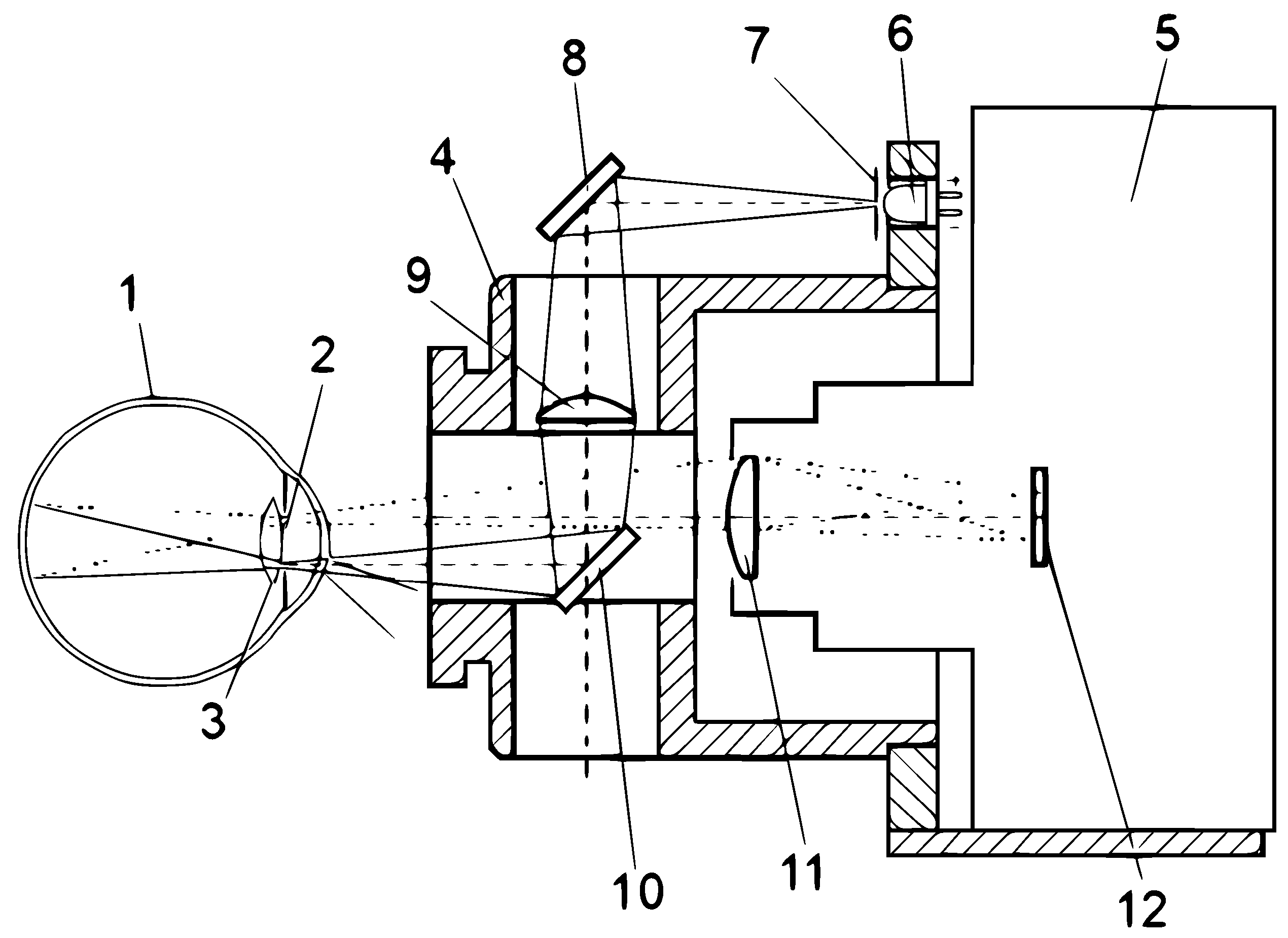
Figure 7.
Optical-electronic system for the analysis of ophthalmic images.
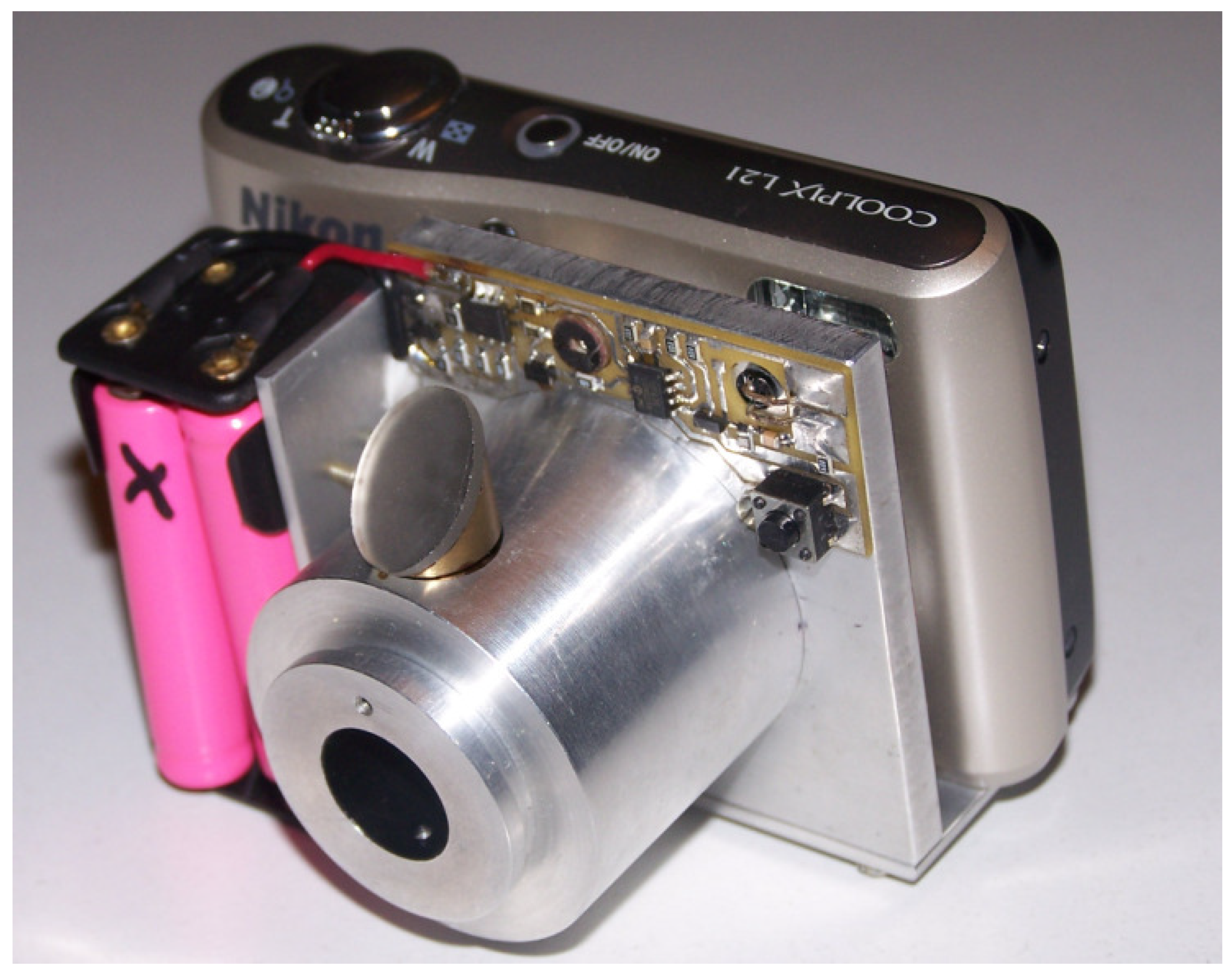
Figure 8.
Image of the retina.
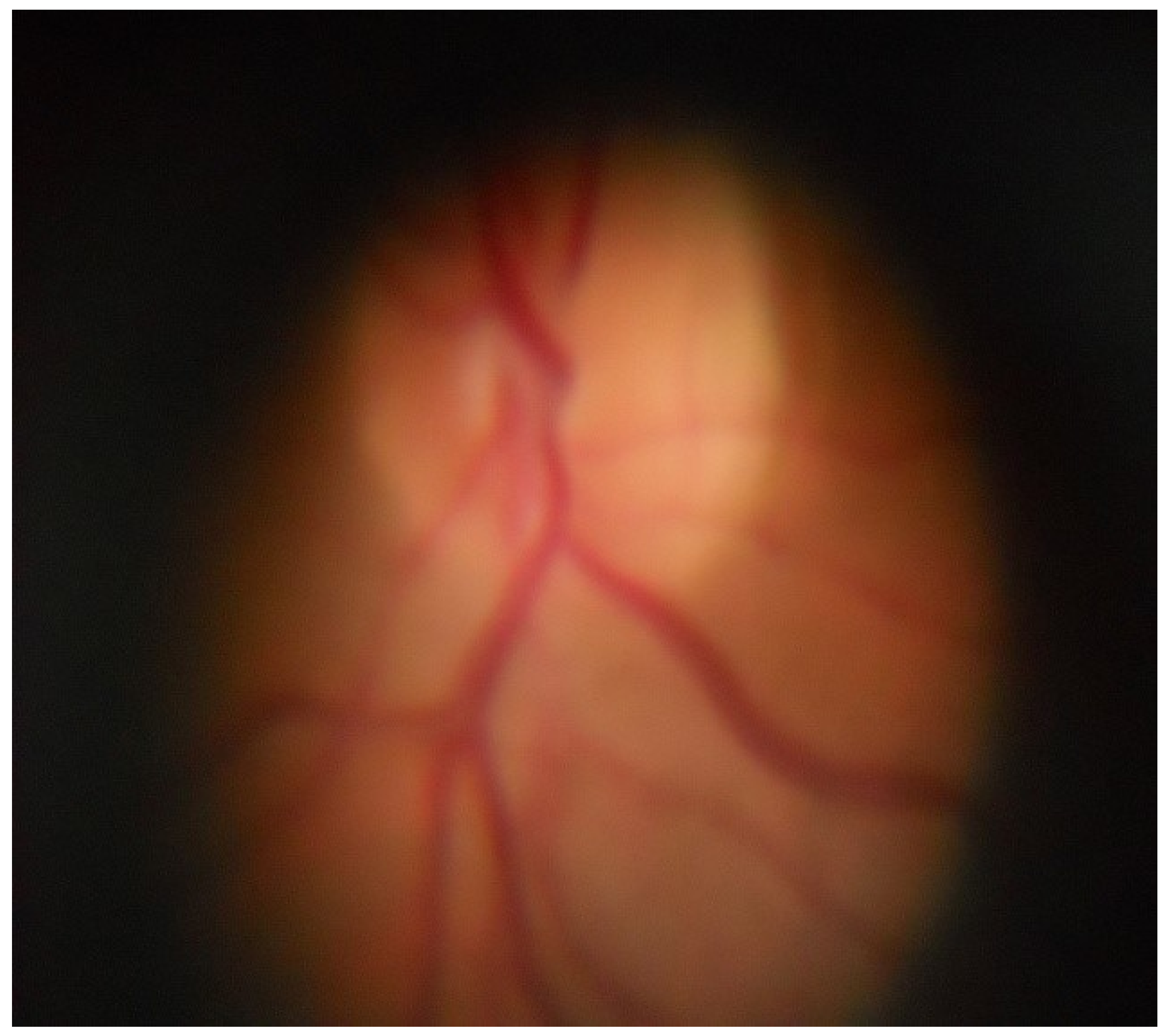
Table 1.
Formation of an expert base in the diagnosis of glaucoma.
| Severity of pathology | Intraocular pressure, mm Hg | Field of vision | Ratio of excavation diameter to OD diameter | Ratio of excavation area to OD area | Ratio of excavation volume to OD volume | Excavation area | Excavation volume | Area of the neuroretinal band | Volume of the neuroretinal girdle | Average thickness of the nerve fiber layer along the edge of the disc | Cross-sectional area of the nerve fiber layer along the edge of the disc |
|---|---|---|---|---|---|---|---|---|---|---|---|
| 31 | |||||||||||
| 33 |
Disclaimer/Publisher’s Note: The statements, opinions and data contained in all publications are solely those of the individual author(s) and contributor(s) and not of MDPI and/or the editor(s). MDPI and/or the editor(s) disclaim responsibility for any injury to people or property resulting from any ideas, methods, instructions or products referred to in the content. |
© 2024 by the authors. Licensee MDPI, Basel, Switzerland. This article is an open access article distributed under the terms and conditions of the Creative Commons Attribution (CC BY) license (http://creativecommons.org/licenses/by/4.0/).
Copyright: This open access article is published under a Creative Commons CC BY 4.0 license, which permit the free download, distribution, and reuse, provided that the author and preprint are cited in any reuse.


