
Submitted:
05 July 2024
Posted:
09 July 2024
You are already at the latest version
Abstract
The heat transfer and fluid mechanics analysis in agitated vessels is usually performed using the Dittus-Boelter correlation. In this study, we propose the analysis of an agitated vessel with a draft tube through the analysis of dimensionless numbers correlations. The heat transfer and fluid mechanics simulation was conducted using ANSYS Fluent software. The simulation used the Sliding Mesh approach and the SST k-ω turbulent model to capture the vessel's fluid flow and heat transfer phenomena. A grid independence study was conducted by varying the number of time steps to obtain an appropriate time step size for the simulation. The convective heat transfer coefficient, as indicated by the mean values of the Nusselt number, was calculated. The local values along the radial coordinate of the heat transfer surface were also determined. These results provide insights into the distribution of heat transfer rates within the vessel, which can help optimize process efficiency and equipment design. The simulation results were analyzed by varying the c and m coefficients in the Nusselt correlation presented as Nu= c Rem Pr1/3. Furthermore, correlations describing the mean Nusselt number at the bottom and wall of the vessel are presented and compared with existing literature, contributing to advancing knowledge in this field.
Keywords:
agitated vessel
; heat transfer
; sliding mesh
; Nusselt number
; CFD
; turbulence model
; correlations
1. Introduction
Mixing vessels are used in numerous industrial processes, where adequate fluid agitation or mixing is crucial for various operations. Agitating fluids serves multiple purposes: mixing two miscible liquids, dissolving solids into liquids, achieving uniform homogenization within a system, and enhancing the efficiency of heat and mass transfer [1].
A draft tube is a cylindrical tube housing an axial flow impeller. In an agitated vessel, the liquid stream produced by the axial-flow impeller strikes the vessel's bottom like a fluid stream exiting a round jet and impacting a flat surface. While there should be some similarities, the primary distinction is the tangential velocity component created by the rotating impeller [2].
Typically, the design of agitated vessels relies on parameters derived from experimental results on laboratory-scale models. While this method is widely adopted, it poses significant cost and construction time issues. Computational Fluid Dynamics (CFD) offers an alternative by enabling preliminary design without the experimental phase, providing parameters to evaluate potential project outcomes.
A typical CFD solver utilizes the finite volume method, which involves discretizing the domain into a finite number of control volumes. General conservation (transport) equations for mass, momentum, energy, and species are then solved within these control volumes. This process converts partial differential equations into a system of algebraic equations, which are ultimately solved numerically to produce the solution field [3].
Some turbulence models are used to simulate the mixing behavior in mixing vessels. The Shear Stress Transport (SST) turbulence model was developed by Florian Menter [4] and initially used for aeronautics applications. However, currently, it is used in some industrial, commercial, and many research codes, as the need for accurate computations of flows with pressure-induced separation, in which the SST model has dramatically benefited from the strength of the underlying turbulence models [5].
Various turbulence models can be used to analyze systems that use Newtonian fluids. In some analyses, the Transition-SST model was the most robust for capturing mixing behavior and reliably predicting separation. Also, it was found that flow predictions within the reactor are particularly sensitive to the turbulence model implemented, and the Transition-SST performed better than k-∊ models in similar mixing problems [6].
It is observed that the k-ω model is noticeably more precise than k-ε in the near wall layers and consequently for flows with moderate adverse pressure gradients but failed for flows with pressure-induced separation [7].
Lane G. analyzed a tank stirred by a Lightning A310 hydrofoil using CFD modeling methods [8]. This analysis modeling used a 3 million nodes mesh and showed that the Shear Stress Transport (SST) turbulence model was better than the k-∊ model for predicting flow structures, but the turbulence was underpredicted. The turbulence predictions were improved using a refined mesh of 28 million nodes and a modified SST model.
The effect of turbulent viscosity in various turbulent models was studied by Tuladhar et al using computational fluid dynamics analyses in an actual gas flow condition inside a cut kerf of a plasma considering various geometric features. This study established the simulation results with the reported experimental measurements and confirmed that the k–ω turbulent model was the most suitable for the used geometry [9].
Ortner et al. investigated the effect of shear stress at the interface between a flowing gaseous phase and a liquid-filled cavity. They analyzed the adverse effect of the resulting quality associated with the simultaneous solution of the transport equations in the turbulence k-ω model in the air and oil regions. They found a way to address this concern by applying a user-defined function (UDF), which sets the turbulent viscosity to zero when an oil volume fraction of 0.9 is exceeded [10].
Benmoussa and Rahmani used a CFD model based on the finite volume method discretization of Navier - Stokes equations to describe the fluid mechanics and heat transfer of yield stress fluid flow with the regularization model of Bercovier and Engelman in a cylindrical vessel equipped with an anchor stirrer. They analyzed the effect of inertia and the influence of plasticity and rheological parameters on hydrodynamic flow behavior, such as the velocity components and power consumption [11].
On the other hand, several turbulence models can simulate systems that include non-Newtonian fluids. Heat transfer during agitation of Bingham viscoplastic fluid was analyzed by Hammami et al. [12]. In this analysis, they tried to identify the rigid zones and optimize mixing and heating performances. They also used the Bingham approximation and Papanastasiou's regularization model to model the fluid rheology. Key results include the presence of recirculation zones and the importance of the anchor position on the size and shape of the rigid zones.
The study of Albertazzi et al. analyzed the emulsification process inside Sulzer Static Mixers. Emulsification is carried out in continuous devices through CFD simulations. They concluded that emulsification offers advantages over batch emulsion, such as better control of the droplet size distribution, reduced volume equipment, and lower operative costs. The analysis of the turbulence model in this application found that the k-∊ turbulence model was more suitable than the k–ω turbulence model. [13].
A Reciprocating-Mechanism Driven Heat Loops (RMDHL) was analyzed by using a CFD solver, including several turbulence models such as realizable k-ɛ models, standard, and SST k-ω models, transition k -ω model, and the transition SST model for the three-dimensional fluid flow. The simulations show that the standard k-ω models provided the least accurate results while the renormalization group (RNG) k-ɛ model provided the most accurate predictions [14].
Tian et al. used the power law model to describe the rheology of pseudoplastic fluids due to its computational stability and low cost [15]. About the turbulence model in pseudoplastics fluids, Wang et al. found that k-ε models outperformed k-ω models in predicting torque characteristics of non-Newtonian flows. Furthermore, Wang et al. found that the SST model was more reliable in predicting velocity profiles and flow patterns in higher-concentration solutions [16].
Based on the analyzed literature, it is observed that the use of the SST k-ω turbulence model is a reasonable option to simulate the heat transfer and fluid dynamics in an agitated vessel with a draft tube, as this turbulence model is used to analyze Newtonian fluids and provide accurate results in CFD models [17]. On the other hand, the SST k-ω turbulence model was also used to analyze the non-Newtonian fluids' mixing characteristics.
The study of Vlček and Jirout investigates heat transfer at the bottom of a cylindrical vessel, where an axial-flow impeller generates a jet within a draft tube. The vertical vessel walls restrict the impinged surface, and a swirling motion is introduced to the liquid flow exiting the draft tube. This study analyzed how this swirling motion impacts bottom heat transfer and provides a dimensionless correlation for the Nusselt number. This swirling motion significantly affects heat transfer, particularly in the stagnant region. Figure 1 shows a typical axial velocity distribution at the draft tube outlet obtained through CFD simulations for this specific geometry [18].
This profile significantly differs from the conventional velocity distribution observed in traditional impinging jets. Adding a tangential velocity component to the primary axial flow and the resulting centrifugal forces causes the peak velocity to shift away from the center. As a result, this shift can lead to a considerable reduction in heat transfer near the stagnation point.
As documented in the literature, many experimental, theoretical, and numerical studies have explored heat transfer in unconfined impinging jets. However, the majority of these studies concentrate on non-swirling flows. The relationship between tangential and axial velocity components is referred to as the swirl number (S), which is defined as follows [19]:
where Gw and Gu represent the axial fluxes of tangential and axial momentums, respectively, and A denotes the outlet cross-sectional area of the draft tube.
The Reynolds number will be used to determine the flow regime, and for agitated vessels, it is defined as follows:
where N is the rotational speed of the impeller in revolutions per second (rev/sec), d is the impeller diameter in meters, and ν is the kinematic viscosity of the fluid. For agitated vessels, the flow regime can be categorized as follows:
Laminar: Re < 50
Transitional: 50 < Re < 5000
Fully Turbulent: Re > 5000
The Nusselt number, which determines the ratio between convective and conductive heat transfer, is defined as:
where α is the heat transfer coefficient of the process, D is the characteristic length (diameter of the vessel), and λ is the thermal conductivity of the fluid. The heat transfer coefficient describes the heat transfer rate between the fluid and the vessel, making it one of the most critical parameters in the process.
In forced convection, the Nusselt number can generally be correlated as follows:
The most common representation of this correlation is the Dittus-Boelter correlation, where the 1/3 power in the Prandtl number is used for cooling [20]. Although it is typically used for flow in a pipe, it can also serve as a useful reference for agitated vessels:
Petera et al. used the electrodiffusion experimental method to measure the heat transfer at the bottom of a cylindrical vessel impacted by a swirling flow from an impeller within a draft tube. They presented the following correlation for the local values of the Nusselt number along the radial coordinate of the heat transfer surface [21]:
Based on the literature analyzed below, several studies have not analyzed the heat transfer and fluid mechanics in an agitated vessel with a draft tube through dimensionless numbers correlations. This study describes a CFD simulation of heat transfer in an agitated vessel with a draft tube based on the study made by Calvopiña H. [22]. The study was performed in ANSYS Fluent using the Sliding Mesh approach and the SST k−ω turbulence model. A grid independence study based on the number of time steps was made to select an appropriate time step size. This analysis includes the mean values and the local values along the radial coordinate of the heat transfer surface of the Nusselt number. The results are validated by comparing them with data from previous simulations. The key findings are the correlations that describe the mean Nusselt number at the agitated vessel bottom and wall, which are also compared with the found in the literature.
This study is organized as follows: Chapter 1 describes previous studies on analyzing the rheology and turbulence models analyzed for different applications. Also, it presents previous correlations analyzed for the study of agitated vessels. Chapter 2 includes the model description and methodology used in this study, including the geometry of the agitated vessel, mesh analysis, and simulation configuration. Chapter 3 describes and analyzes this study's primary results, including correlations under a specific rotation velocity, heat transfer, and nondimensional numbers that describe the physical phenomena. Finally, Chapter 4 shows the main findings of this study.
2. Materials and Methods
Several rotational speeds were simulated in ANSYS Fluent, using the SST k−ω turbulence model with the Kato-Launder correction activated [23]. The geometry consisted of an agitated vessel with a six-blade impeller (blades pitched at 45°) placed inside a draft tube, and the fluid used was water at a temperature of 300 K. The bottom and walls of the vessel were subjected to a constant heat flux of 30000 W/m². Figure 2 illustrates the geometrical configuration of the model along with its dimensions.
The mesh comprised more than 3 million elements. The simulation script was divided into three parts. Initially, steady-state iterations were performed with the energy equation turned off. Following this, the simulations switched to a transient model using the Sliding Mesh approach. In this phase, 4 seconds was simulated without the energy equation to establish an initial transient velocity field. Finally, 20 seconds were simulated with the energy equation activated and a constant heat flux of 30000 W/m² applied.
The mesh initially created in ANSYS Mesh was refined in ANSYS Fluent by converting the tetrahedral mesh elements into polyhedral elements. This adjustment reduced the number of elements from approximately 3 million to 2 million and improved the orthogonal quality (which ranges from 0 to 1, with values close to 0 indicating low quality) from 0.072 to 0.28, and the maximum skewness was 0.71. The height of the first layer of the mesh at the bottom of the tank (inflation layer) was defined as 0.4 mm in ANSYS Mesh.
When we are interested in heat transfer, the whole viscous sublayer must be appropriately described, and no wall functions should be used in such cases. In order to accomplish this, the Y+ value should be close to 1. After performing the simulations, it was verified that the values of Y+ satisfied this condition. Figure 3 shows the Y values at the bottom and wall for a rotational speed of 900 RPM.
The study on the number of mesh elements for an agitated vessel was previously conducted by Chakravarty A [24]. Therefore, a grid independence study was performed focusing on the number of time steps. This study aimed to select an appropriate time step, balancing accuracy with simulation time. The results of three simulations with a rotational speed of 500 RPM were evaluated. The outcomes are presented in Table 1.
3. Results and Discussion
The Grid Convergence Index (GCI) was calculated using MATLAB. The monitored quantity was the total Heat Transfer Coefficient (HTC), and the number of time steps was evaluated only for the final 20 seconds (when the energy equation was activated). Figure 4 illustrates the relationship between the Heat Transfer Coefficient and the number of time steps for a rotational speed of 500 RPM.
The results of the GCI analysis exhibit a non-monotonic dependency of the monitored quantity on the number of time steps, showing an oscillatory tendency with non-decreasing amplitude. Specifically, the GCI for the highest number of time steps (20,000) is smaller for the middle point (4,000) but larger for the smallest number of time steps (2,000). This behavior could be attributed to the time step size; a much smaller time step should ideally be used for the Sliding Mesh approach. However, these results complicate the proper evaluation of the GCI concerning the number of time steps.
The primary parameter for selecting the time step size was the duration required to complete the simulation. A simulation with a time step of 0.01 seconds took approximately 3 to 5 days on the computational servers at the Czech Technical University, using an ELF - HP ProLiant DL560 G8, 4 processors Intel Xeon E5-4620 v2, 32 cores in total, 2.6 GHz, and 256 GB RAM. Reducing the time step to 0.005 seconds for the same simulation would increase the duration to 8 to 10 days. Given that multiple simulations were needed to analyze the results, a time step of 0.01 seconds was chosen to balance accuracy and computational efficiency.
The material used in this simulation is water with constant properties (no temperature dependence), and the primary boundary condition is a constant heat flux of 30000 W/m2. After determining the appropriate time step size, simulations were conducted for eight rotational speeds ranging from 200 to 900 RPM. The evaluated parameter was the mean Nusselt number. Since the bottom and wall of the tank are heated simultaneously, three different Nusselt numbers were calculated: one for the bottom, one for the wall, and a total Nusselt number, which is the average of the previous two. Table 2 presents the mean Nusselt numbers obtained from the simulations and the corresponding Reynolds numbers, calculated using the dynamic viscosity (μ=0.001003 Pa s) and density (ρ=998.2 kg/m3) of water, as given by Equation 4.
With the data obtained from the simulations, the goal was to present a correlation for the Nusselt number as follows:
Nonlinear regression was conducted using MATLAB functions nlinfit and nlparci to determine the coefficients C and m for the abovementioned correlation. Table 3 presents the values of these coefficients, C and m, along with their confidence intervals, which indicate the ranges where the best-fit parameter values lie with 95% probability for the Nusselt number at the bottom, at the wall, and the total.
The correlations can be outlined as follows:
The Nubottom correlation was compared with other published correlations, the Dittus-Bolter correlation [25], the Petera et al. correlation [21], and the Moving Reference Frame (MRF) correlation [21]. The cited correlations and the confidence zone, limited by dashed lines, are shown in Figure 5. As is observed in this figure the proposed correlation is located in the confidence zone.
Figure 6 illustrates the relationship between the Nusselt number and the Reynolds number for the correlations obtained through nonlinear regression, the Dittus-Boelter correlation (Equation 7), and the data obtained from the simulation for the bottom, the wall, and the total.
We can observe from the data in Table 3 that the exponents of the Reynolds number in the correlations are pretty large, particularly for the bottom, which has a value of 1.059 with a confidence interval between 0.903 and 1.215, indicating an error of about 15%. For the correlation at the wall, the exponent of the Reynolds number obtained from the regression is similar to the exponent in the Dittus-Boelter correlation, but the confidence interval remains significant, with an error of about 30%. Therefore, another nonlinear regression was performed to compare the simulation results with the exact Dittus-Boelter correlation. This time, only the constant c was calculated, while the exponent of the Reynolds number was fixed at 0.8. Table 4 presents the value of the coefficient c and its confidence interval for the Nusselt number at the bottom, the wall, and the total.
The correlations can be outlined as follows:
The new correlations have a more substantial impact at the bottom, where the coefficient of 0.03 is very close to the coefficient in the Dittus-Boelter correlation (0.023), and the error decreases from 15% to 10%. For the wall, although the coefficient did not change significantly (from 0.010 to 0.014), the confidence interval decreased notably, reducing the error from 30% to around 10%. Figure 7 shows the relationship between the Nusselt number and the Reynolds number for the new correlations at the bottom, wall, and total compared with the Dittus-Boelter correlation.
The local values of the Nusselt number at the bottom were measured for different Reynolds numbers along the dimensionless radial coordinate r/d, where r is the tank's radius and d is the diameter of the draft tube. Figure 8 presents the results.
We can observe that the highest value of the Nusselt number (and thus the heat transfer coefficient) is not at the center of the tank but approximately at the radial dimensionless coordinate r/d = 1. This shift is attributed to the tangential velocity, distinguishing this setup from non-swirling impinging jets, where the highest heat transfer coefficient is typically found closer to the tank's center (r/d = 0).
However, Petera et al. [21] published an experimental study on heat transfer at the bottom of an agitated vessel for different dimensionless distances h/d. They found that the impact of tangential velocity is more significant at smaller distances from the bottom of the vessel and is minimal at a dimensionless distance h/d = 1, which is the scenario in the present study.
Concerning the wall, the local values of the Nusselt number were measured for different rotational speeds along the dimensionless coordinate y/H, where y is the distance from the bottom, and H is the height of the tank. A significant increase was observed starting from 400 RPM (Re = 25000); the local values can be considered constant at lower rotational speeds. The highest value is located at the corner (y/H close to 0), which is caused by the presence of a swirl, enhancing the convective heat transfer. This behavior is similar to the local values of the Nusselt number along a flat plate, where, theoretically, the heat transfer coefficient is infinitely large at the beginning. We do not have an infinitely sizeable Nusselt number, but the peak is located at the start. Figure 9 shows the dependence of the local Nusselt number values on different rotational speeds.
Another simulation at 500 RPM with a time step of 0.01 seconds was performed, but only the bottom was heated in this case. This simulation was conducted to compare the effects of the boundary conditions. In this project, the bottom and the wall are heated simultaneously, whereas experimental results typically heat the bottom and the wall separately. The average heat transfer coefficient when only the bottom is heated was 2136.80 W/m²K; when both the bottom and wall are heated simultaneously, it was 2025.59 W/m²K. Comparing these values reveals a difference of approximately 5%. The results of the local values of the Nusselt number along the dimensionless coordinate r/d are shown in Figure 10.
The main difference is in the corner where the bottom and wall meet. In the corner, due to the centrifugal forces generated by the impeller, the fluid stream is impinging the wall perpendicularly. Therefore, the width of the thermal boundary layer decreases, which means a higher heat transfer coefficient. The radial component of the velocity decreases when the radius increases. The Nusselt number is significantly higher in the corner when only the bottom is heated. The latter is due to the more significant temperature difference between the bottom and wall, resulting in a higher heat transfer coefficient. The velocity profile of the model simulation is presented in Figure 11.
The mean values of the Nusselt number at the bottom obtained from our simulations were compared with existing data from a simulation using the MRF (Moving Reference Frame) approach, where only the bottom was heated [21], [26]. The time step used in the MRF simulation was the same as in our simulations (0.01 sec). The correlation obtained from this MRF simulation was:
The confidence interval for the exponent of the Reynolds number was 0.680 ± 0.051, and for the leading constant, it was 0.101 ± 0.055. Comparing this data with Equation 7, we observe that the leading constant and the Reynolds exponent from the MRF approach correlation differ and fall outside the confidence intervals of the values obtained with the Sliding Mesh approach.
The different boundary conditions could be one reason for these discrepancies, particularly the Reynolds number exponent. The Sliding Mesh approach simulations were conducted with heat flux applied to both the bottom and wall simultaneously, whereas the MRF approach simulations had heat flux applied only to the bottom. Another, and likely the primary reason, is the size of the time step. The Sliding Mesh approach is more sensitive to time step size, requiring it to be sufficiently small.
Figure 12 shows the mean Nusselt number values for various Reynolds numbers obtained using the MRF and Sliding Mesh approaches and the correlation from Equation 7 obtained via nonlinear regression.
The dashed lines represent the prediction bands of the correlation from Equation 7; this region indicates where 95% of the data points would fall if additional data were collected and measured.
Most of the data obtained with the MRF approach falls within the prediction bands, which, from a statistical perspective, indicates that the compared data is similar.
The final temperature can be calculated analytically and compared with the results from the simulation. This comparison allows us to determine if the simulation behaves appropriately and if the results are reliable from a physical perspective.
We can start by calculating the heat flux using the following equation:
where m is the total mass of the heated fluid, which can be calculated as the tank's volume times the water's density (998 kg/m3). The specific heat capacity (Cp) is constant for water, with a 4182 J/kg·K value. A heat flux of 30000 W/m2 was used (q), so we need to consider the surface area where the heat flux was applied (S). Therefore, the previous equation can be expressed as:
This equation is an ordinary differential equation that can be solved by separating and integrating the variables. The integration limits for the temperature are from the known initial temperature (300 K) to the final temperature (Tf) and for the time, from 0 to 20 seconds. The heat flux, surface area, tank volume, water density, and specific heat capacity of water remain constant.
The heat flux is applied to both the bottom and the wall; thus, the surface area (S) is the sum of the bottom surface area (πr2) and the wall surface area (2πr × H). The diameter of the tank is 392 mm, and the height of the tank is 430 mm. Therefore, the total surface area (S) is 0.65 m², and the volume of the tank (πr2 × H) is 0.05 m³. By substituting these values into Equation 19, the final temperature (Tf) is calculated as 301.86 K. The final temperature obtained from the simulation, using a report of volume integrals, is 301.82 K, thus confirming the accuracy of the calculation.
Two additional simulations were conducted at 500 RPM with the same boundary conditions (bottom and wall heated simultaneously) and a time step of 0.01 seconds but with extended mixing times of 30 and 40 seconds. The latter was done to compare the accuracy of the current results (with a 20-second mixing time) against the results from simulations with longer mixing times.
The comparison was conducted using a similar approach to the grid convergence study performed in MATLAB. The grid convergence indexes (GCI) were calculated for the Nusselt number at the bottom, wall, and total. A decreasing trend was observed in all values. The GCI results with a 20-second mixing time were 8% for the Nusselt number at the bottom, 12% at the wall, and 21.07% for the total Nusselt number.
Table 5 presents the results of the Nusselt number according to the mixing time, along with all the GCI values and the Nusselt number's extrapolated values at the bottom, wall, and total.
A correction must be applied for a considerably longer mixing time to account for the temperature increase of the fluid in the vessel. For calculating the heat transfer coefficient (α), the Fluent solver does not consider this temperature increase but instead takes the fluid temperature as a constant input parameter (Tref) according to the following equation:
where Tw is the temperature at the wall, and q is the heat flux.
In this study, no correction was necessary because the temperature increase of the fluid after mixing was relatively small (1.82 K).
The monitored quantity exhibits a non-monotonic dependence on the number of time steps, with the GCI results showing an oscillatory trend of non-decreasing amplitude. Specifically, the GCI for the largest number of time steps (20000) is less than the GCI for the middle point of time steps (4000) but greater than the GCI for the fewest number of time steps (2000).
There is an error of approximately 15%, with correlations being too large at values of 1.059 and a confidence interval of 0.903 to 1.125. The Reynolds number exponent obtained from the regression is similar to the exponent from the Dittus-Boelter correlation, though it has a large confidence interval and an error of approximately 30%.
We used MATLAB to calculate the convergence index for the Nusselt number at the bottom, wall, and total, with a decreasing trend identified in all values. The GCI results with a 20-second mixing time were 8% for the Nusselt number at the bottom, 12% for the wall, and 21.07% for the total.
4. Conclusions
Using the SST k–ω turbulence model with the Kato-Launder correction and the sliding mesh approach, heat transfer was analyzed in a stirred vessel with a draft tube at various rotation speeds ranging from 200 to 900 RPM. The sliding mesh approach was assumed to provide higher accuracy than the moving reference frame (MRF) approach, with mesh modification in ANSYS Fluent employed to improve mesh quality.
A grid independence study determined the appropriate time range for the simulations. It was observed that the grid convergence index (GCI) exhibited an oscillatory trend with non-decreasing amplitude. Consequently, a suitable GCI value could not be reliably evaluated based on the entire simulation duration, which ranges from 3 to 5 days with a time step of 0.01 seconds.
The correlation for the mean Nusselt number was evaluated for the bottom, the wall, and the total. The Dittus-Boelter correlation was compared using nonlinear regressions in MATLAB, and the respective coefficients were determined.
Local Nusselt number values were evaluated at the vessel's bottom and wall. At the bottom, a peak occurs where r/d is approximately 1. On the wall, the highest value is near the corner, where y/H is close to 0.
The previous simulations were compared with the mean Nusselt number values results obtained using the Moving Reference Frame (MRF) approach. Similar Nusselt number values were found in both cases, specifically within the Reynolds number range of 3000 to 4000.
The influence of simulation time on the accuracy of results was evaluated using an approach similar to the grid convergence study. The difference in accuracy between the actual and extrapolated values for the 20-second mixing time was 8% at the bottom and 12% at the wall.
The Sliding Mesh approach requires a much smaller time step to obtain more accurate results. However, repeating the simulations with a more minor time step was impossible due to the high computational requirements.
Increasing the mixing time could increase the accuracy of the results, albeit at the cost of extended simulation time. A correction to eliminate the temperature increase of the liquid in the vessel would be necessary when this effect cannot be neglected, as demonstrated in the study by Chakravarty A. [24].
Some different turbulence models could be employed to perform new simulations and compare the results with those obtained in the present work. Furthermore, it would be possible to reach more accurate results using a more minor time step in the sling mesh approach. All of these improvements must be applied in future analysis.
Author Contributions
Conceptualization, Hector Calvopiña; methodology, Hector Calvopiña; software, Fidel Castro; validation, David Balseca; formal analysis, Benjamin Velastegui; visualization, José Gallardo; writing—original draft preparation, Hector Calvopiña; writing—review and editing, Francisco Paredes; supervision Francisco Montero. “All authors have read and agreed to the published version of the manuscript.”.
Data Availability Statement
The data used in this study can be found at http://hdl.handle.net/10467/77657.
Acknowledgments
Hector Calvopiña would like to express his gratitude to the SENESCYT for granting him a scholarship, which allow him to obtain a master's degree.
Conflicts of Interest
“The authors declare no conflicts of interest”.
References
- Geankoplis, C.J.; Hersel, A.A.; Lepek, D.H. Transport Processes and Separation Process Principles. in Prentice Hall international series in the physical and chemical engineering sciences. Prentice Hall, 2018. [Online]. Available: https://books.google.com.ec/books?
- Petera, K.; Dostál, M.; Rieger, F. “Transient measurement of heat transfer coefficient in agitated vessel,” Czech Technical University in Prague, no. 2, 2008.
- Ansys, “What is Computational Fluid Dynamics (CFD)?,” https://www.ansys.com/simulation-topics/what-is-computational-fluid-dynamics.
- Ferrari, S.; Rossi, R.; Di Bernardino, A. “A Review of Laboratory and Numerical Techniques to Simulate Turbulent Flows,” Energies (Basel), vol. 15, no. 20, 2022. [CrossRef]
- Langtry, R.; Menter, F. “Transition Modeling for General CFD Applications in Aeronautics,” in 43rd AIAA Aerospace Sciences Meeting and Exhibit, in Aerospace Sciences Meetings., American Institute of Aeronautics and Astronautics, 2005. [CrossRef]
- Coughtrie, A.R.; Borman, D.J.; Sleigh, P.A. “Effects of turbulence modelling on prediction of flow characteristics in a bench-scale anaerobic gas-lift digester,” Bioresour Technol, vol. 138, pp. 297–306, Jun. 2013. [CrossRef]
- Menter, F. “Zonal Two Equation k-w Turbulence Models For Aerodynamic Flows,” in 23rd Fluid Dynamics, Plasmadynamics, and Lasers Conference, in Fluid Dynamics and Co-located Conferences., American Institute of Aeronautics and Astronautics, 1993. [CrossRef]
- Lane, G.L. “Improving the accuracy of CFD predictions of turbulence in a tank stirred by a hydrofoil impeller,” Chem Eng Sci, vol. 169, 2017. [CrossRef]
- Tuladhar, U.; et al. “Numerical Modeling of an Impinging Jet Flow inside a Thermal Cut Kerf Using CFD and Schlieren Method,” Applied Sciences (Switzerland), vol. 12, no. 19, 2022. [CrossRef]
- Ortner, B.; Schmidberger, C.; Prieler, R.; Mally, V.; Hochenauer, C. “Analysis of the shear-driven flow in a scale model of a phase separator: Validation of a coupled CFD approach using experimental data from a physical model,” International Journal of Multiphase Flow, vol. 177, p. 104852, 2024. [CrossRef]
- Benmoussa, A.; Rahmani, L. “Numerical analysis of thermal behavior in agitated vessel with non-Newtonian fluid,” International Journal of Multiphysics, vol. 12, no. 3, 2018. [CrossRef]
- Hammami, M.; Chebbi, A.; Baccar, M. “Numerical study of hydrodynamic and thermal behaviors of agitated yield-stress fluid,” Mechanics and Industry, vol. 14, no. 4, 2013. [CrossRef]
- Albertazzi, J.; Florit, F.; Busini, V.; Rota, R. “CFD modeling of emulsions inside static mixers,” Chem Eng Sci, vol. 294, p. 120082, 2024. [CrossRef]
- Popoola, O.; Cao, Y. “The influence of turbulence models on the accuracy of CFD analysis of a reciprocating mechanism driven heat loop,” Case Studies in Thermal Engineering, vol. 8, 2016. [CrossRef]
- Tian, F.; Zhan, X.; He, H.; Liu, S.; Yang, T.; Xiao, H. “A modified lumped capacitance method for transient heat transfer in a stirred tank with non-Newtonian fluid,” Appl Energy, vol. 368, p. 123483, 2024. [CrossRef]
- Wang, P.; Reviol, T.; Ren, H.; Böhle, M. “Effects of turbulence modeling on the prediction of flow characteristics of mixing non-Newtonian fluids in a stirred vessel,” Chemical Engineering Research and Design, vol. 147, 2019. [CrossRef]
- Romano, M.G.; Alberini, F.; Liu, L.; Simmons, M.J.H.; Stitt, E.H. “Comparison between RANS and 3D-PTV measurements of Newtonian and non-Newtonian fluid flows in a stirred vessel in the transitional regime,” Chem Eng Sci, vol. 267, p. 118294, 2023. [CrossRef]
- Vlček, P.; Jirout, T. “CFD simulation of flow in mixing equipment with draft tube,” in CHISA conference, Seč, Czech Republic, 2015.
- Ward, J.; Mahmood, M. “Heat transfer from a turbulent, swirling, impinging jet,” in Heat Transfer 1982, Volume 3, Jan. 1982, pp. 401–407.
- Tosun, I. “4 - EVALUATION OF TRANSFER COEFFICIENTS: ENGINEERING CORRELATIONS,” in Modeling in Transport Phenomena (Second Edition), I. Tosun, Ed., Amsterdam: Elsevier Science B.V., 2007, pp. 59–115. [CrossRef]
- Petera, K.; Dostál, M.; Vìøíšová, M.; Jirout, T. “Heat Transfer at the bottom of a cylindrical vessel impinged by a swirling flow from an impeller in a draft tube,” Chem Biochem Eng Q, vol. 31, no. 3, 2017. [CrossRef]
- Héctor, C. “CFD simulation of heat transfer in an agitated vessel with a draft tube,” http://hdl.handle.net/10467/77657.
- Kato, M.; Launder, B.E. “The modeling of turbulent flow around stationary and vibrating square cylinders,” Ninth Symposium on Turbulent Shear Flows, no. January 1993. 1993. [Google Scholar]
- Chakravarty, A. “CFD Simulation of Heat Transfer in an Agitated Vessel,” M.sc thesis in CZECH TECHNICAL UNIVERSITY IN PRAGUE, 2017.
- Dittus, F.W.; Boelter, L.M.K. “Heat transfer in automobile radiators of the tubular type,” International Communications in Heat and Mass Transfer, vol. 12, no. 1, pp. 3–22, 1985. [CrossRef]
- Petera, K. “Momentum, Heat and Mass Transfer,” https://moodle-vyuka.cvut.cz/course/info.php?id=1536.
Figure 1.
Example of typical axial and tangential velocity profiles at the draft tube outlet [18].
Figure 1.
Example of typical axial and tangential velocity profiles at the draft tube outlet [18].
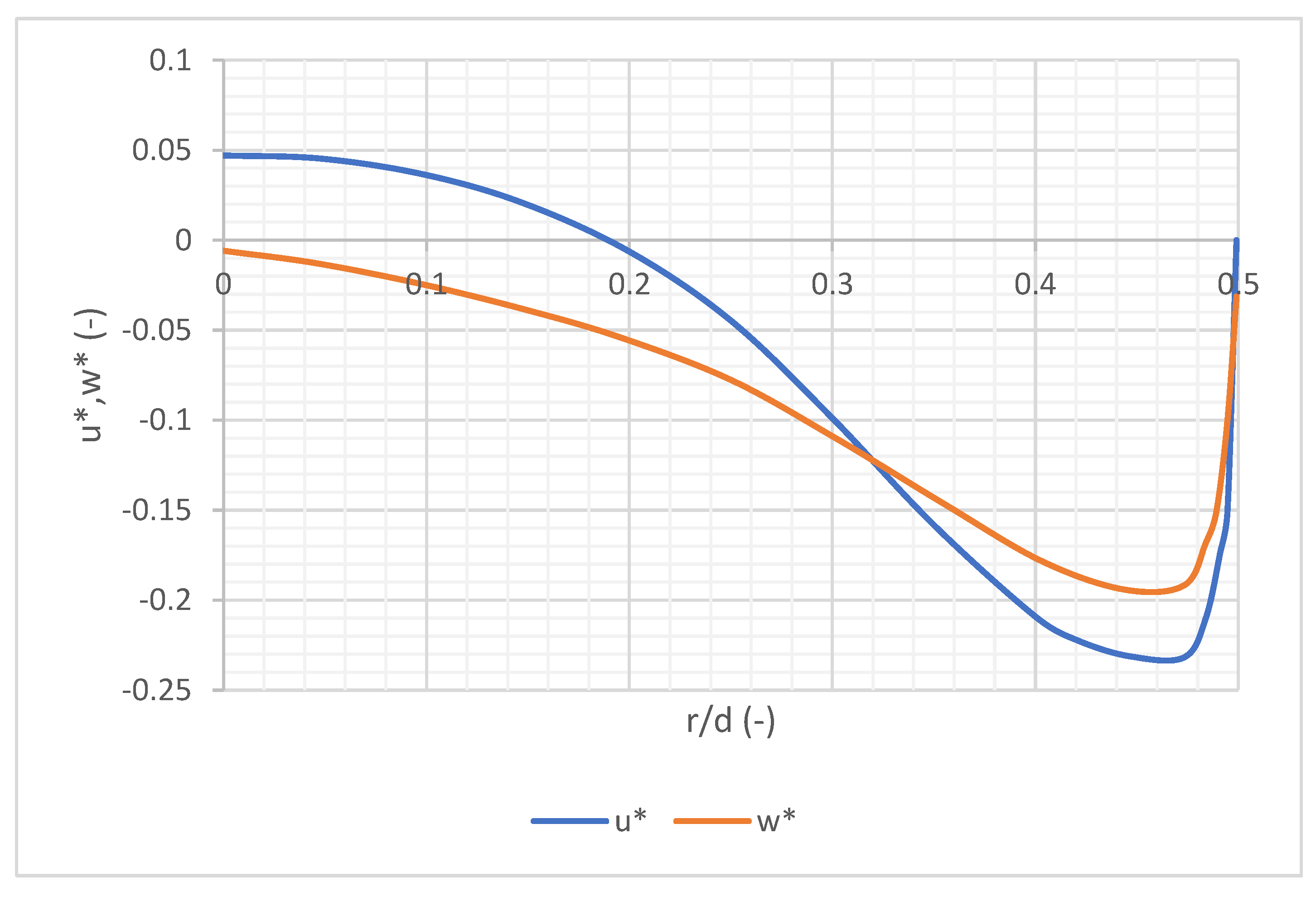
Figure 2.
Geometrical configuration of the model [22].
Figure 2.
Geometrical configuration of the model [22].
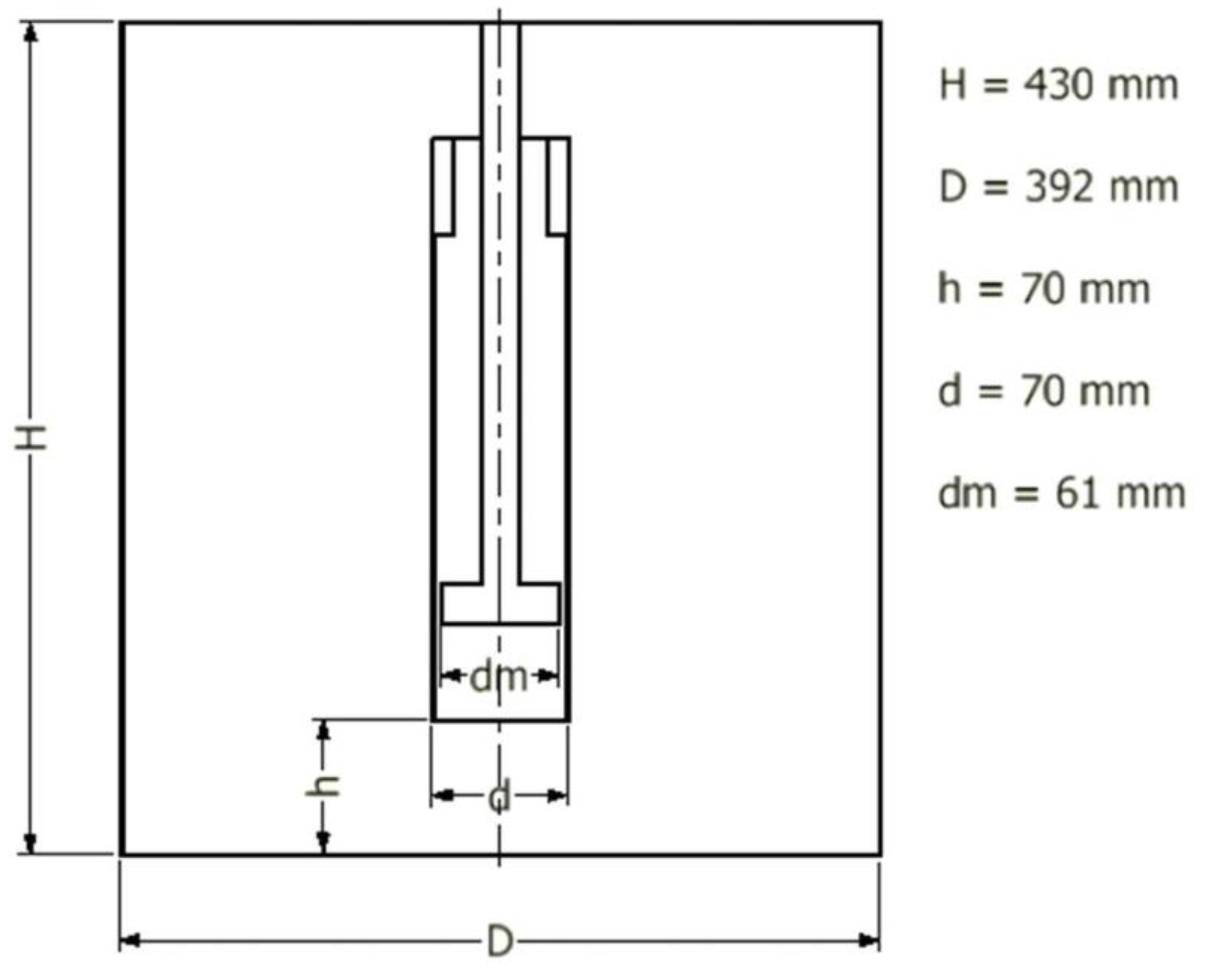
Figure 3.
(a) Values of Y+ at the bottom of the tank, (b) Values of Y+ at the wall of the tank [22].
Figure 3.
(a) Values of Y+ at the bottom of the tank, (b) Values of Y+ at the wall of the tank [22].
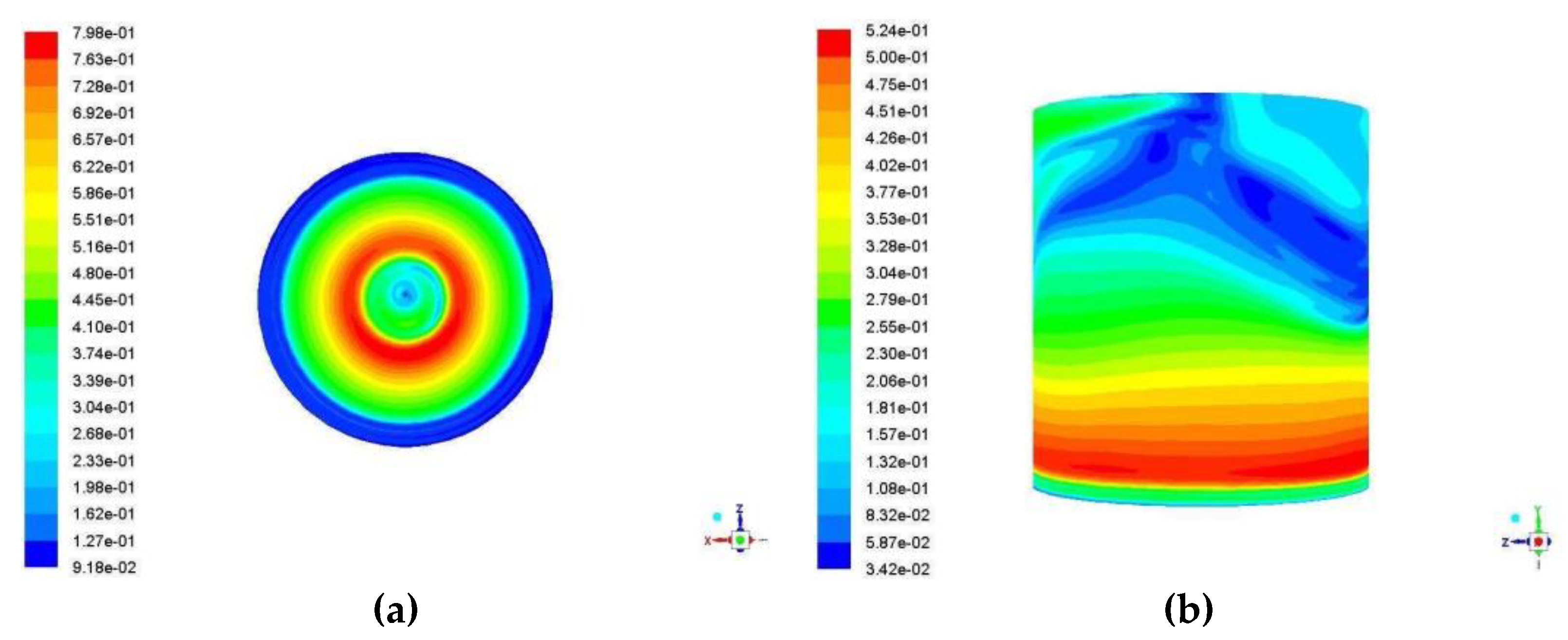
Figure 4.
Dependence of the HTC on the number of time steps for 500 RPM [22].
Figure 4.
Dependence of the HTC on the number of time steps for 500 RPM [22].
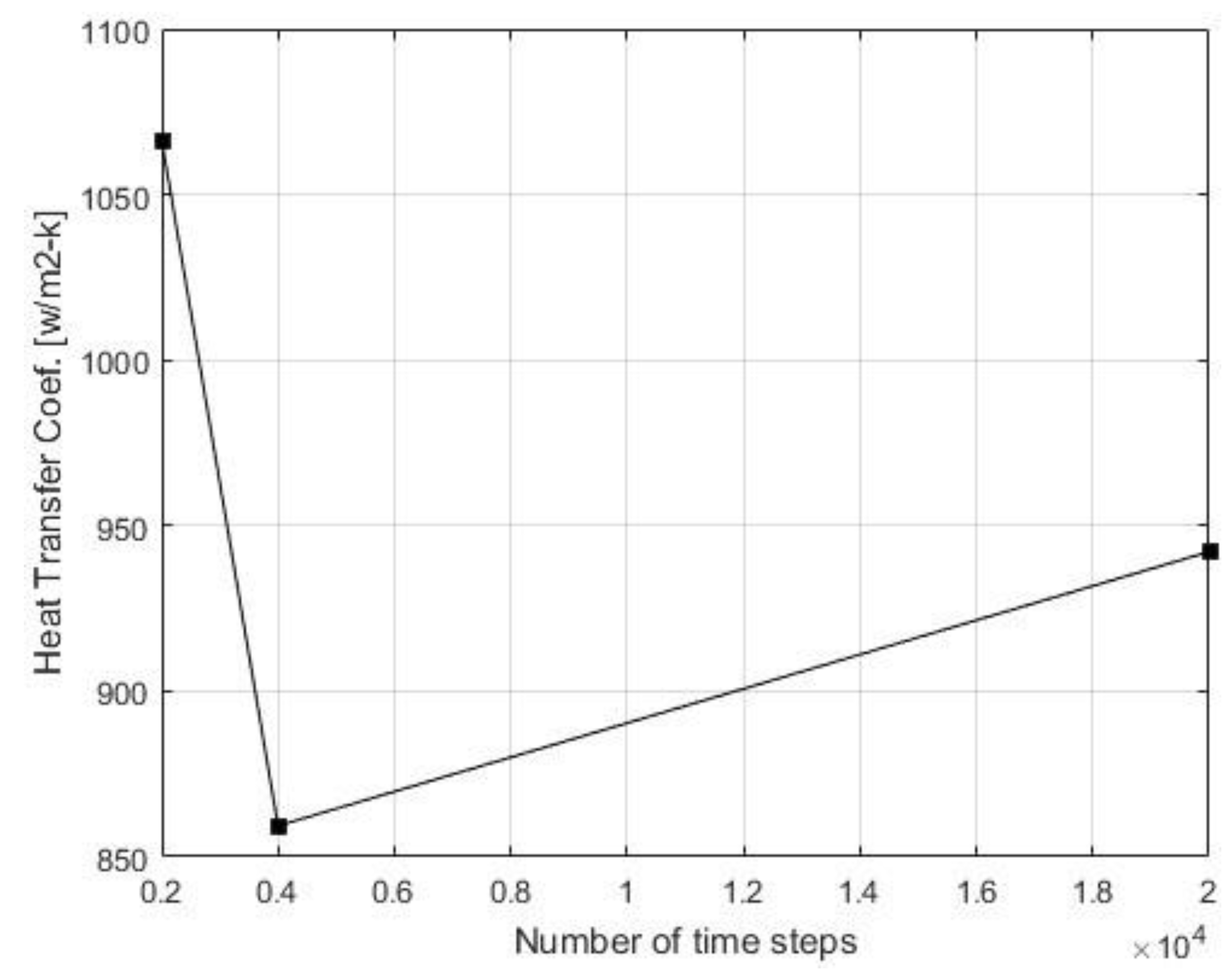
Figure 5.
Nu correlation for the bottom of the simulated vessel compared with the previously published Nu correlations [22].
Figure 5.
Nu correlation for the bottom of the simulated vessel compared with the previously published Nu correlations [22].
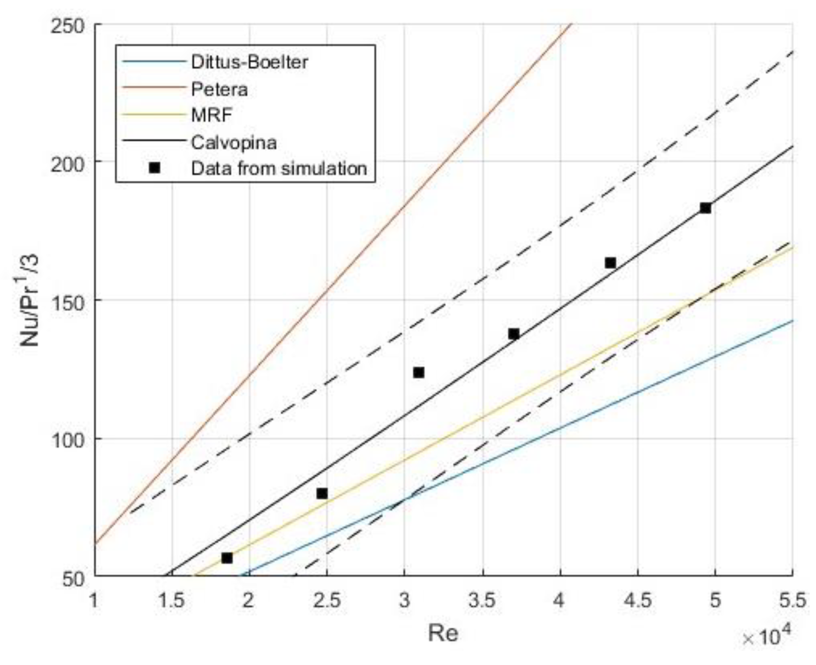
Figure 6.
Correlations obtained from the nonlinear regression, the simulation data, and the Dittus-Boelter correlation from the literature as a function of Reynolds number, for (a) bottom of the vessel, (b) wall of the vessel, and (c) total [22].
Figure 6.
Correlations obtained from the nonlinear regression, the simulation data, and the Dittus-Boelter correlation from the literature as a function of Reynolds number, for (a) bottom of the vessel, (b) wall of the vessel, and (c) total [22].
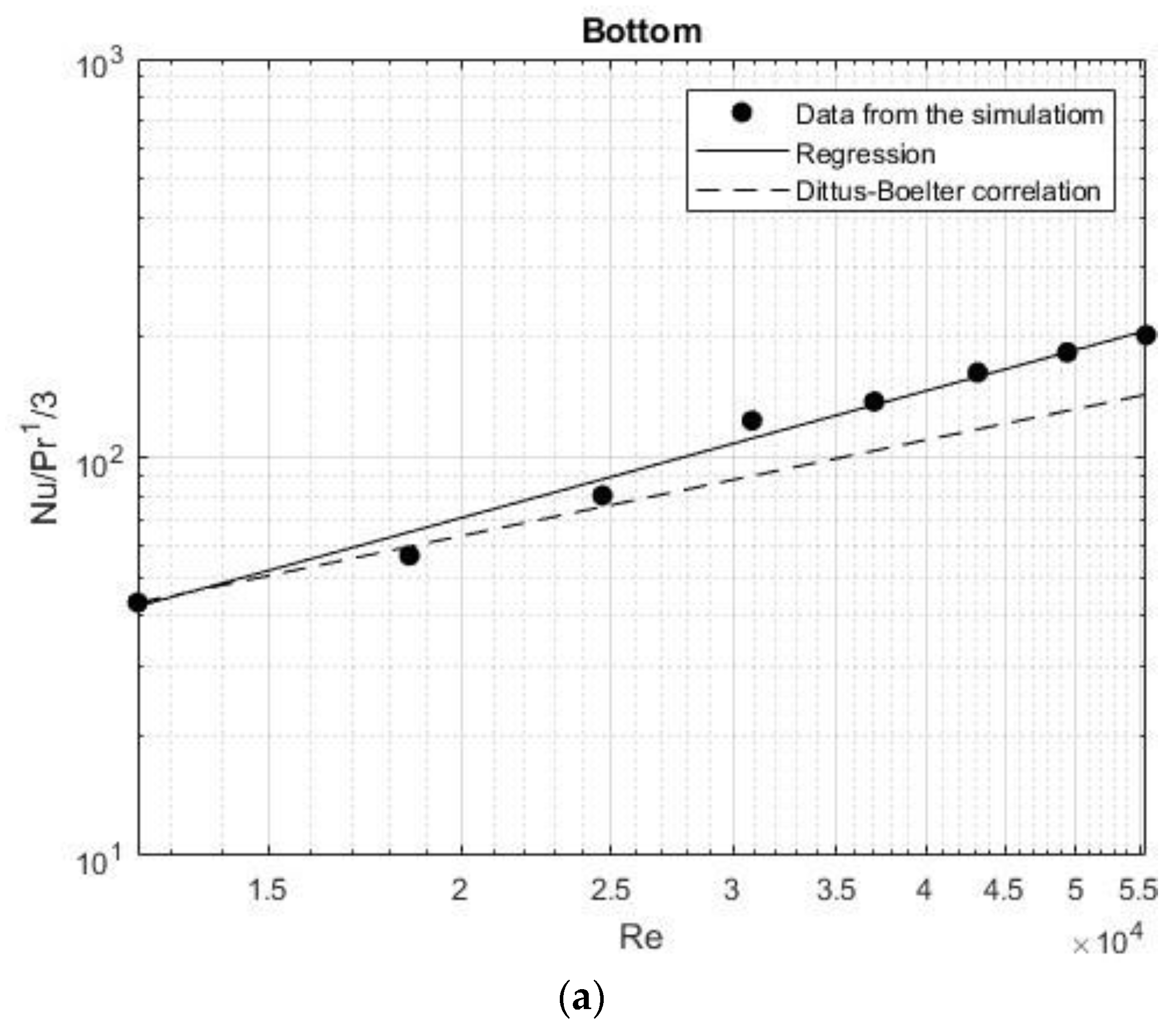
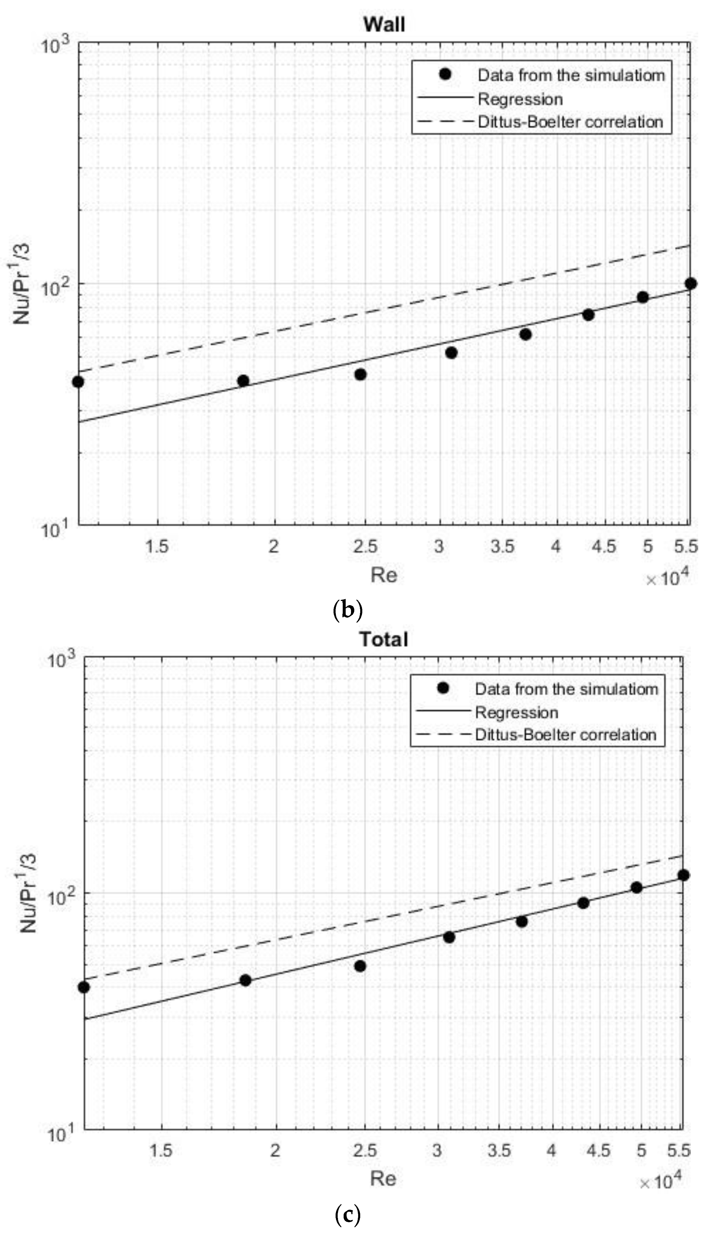
Figure 7.
Correlations obtained from the second nonlinear regression (only the parameter c was calculated, and the exponent of the Reynolds number used was 0.8) and data from the simulation are compared with the literature correlation of Dittus-Boelter, for a) bottom of the vessel, b) wall of the vessel, and c) total [22].
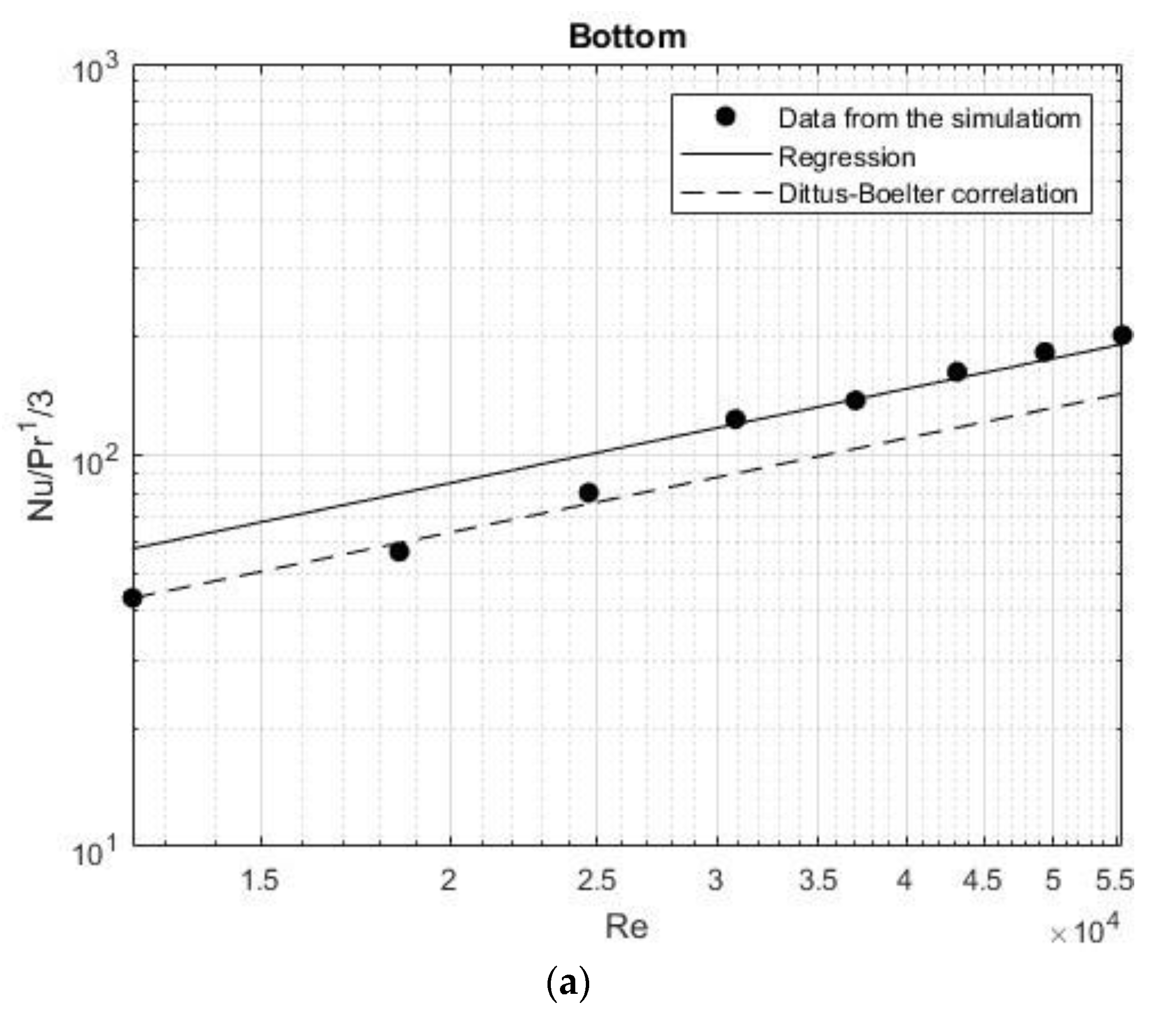
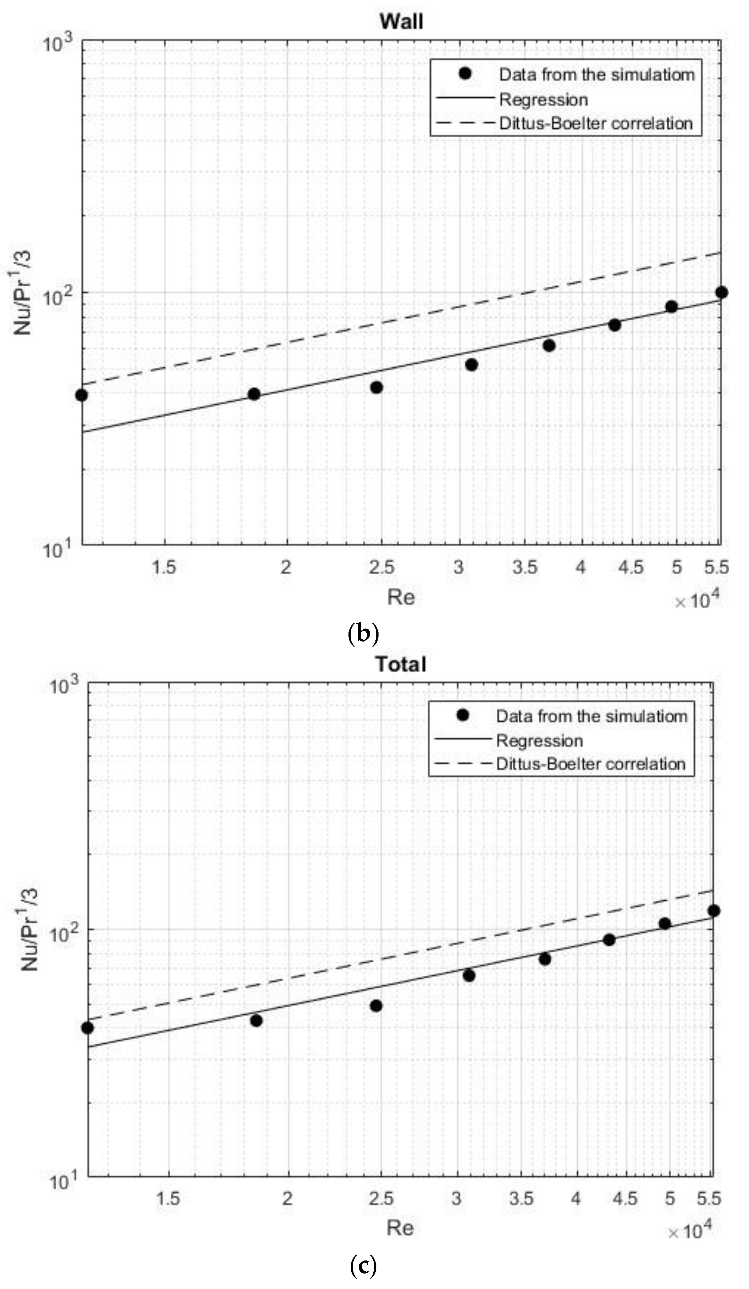
Figure 8.
Local values of the Nusselt number at the bottom for different Reynolds numbers along the dimensionless coordinate r/d [22].
Figure 8.
Local values of the Nusselt number at the bottom for different Reynolds numbers along the dimensionless coordinate r/d [22].
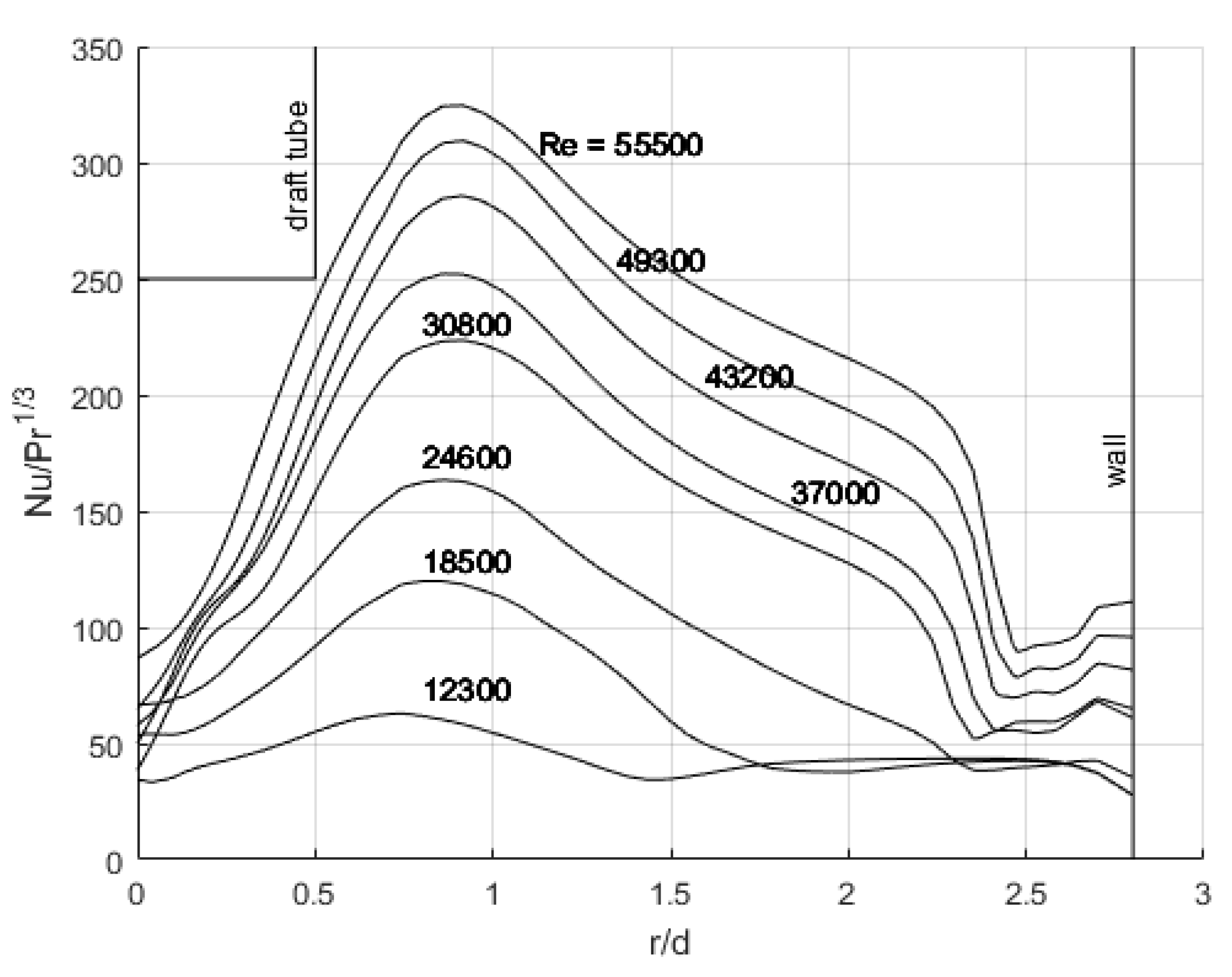
Figure 9.
Local values of the Nusselt number at the wall along the dimensionless coordinate y/H [22].
Figure 9.
Local values of the Nusselt number at the wall along the dimensionless coordinate y/H [22].
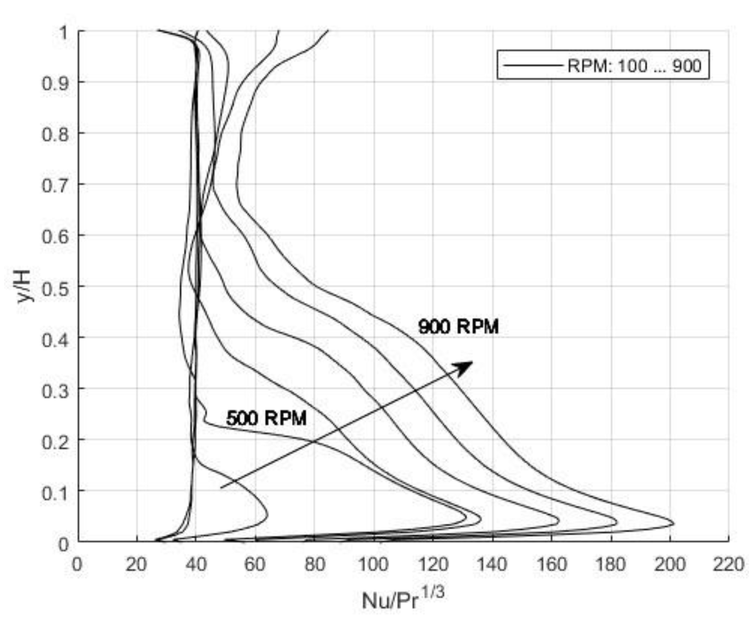
Figure 10.
Local values of the Nusselt number at the bottom along the dimensionless coordinate r/d for two different simulations: only the bottom is heated, and the bottom and wall are heated simultaneously (500 RPM, Re = 30000) [22].
Figure 10.
Local values of the Nusselt number at the bottom along the dimensionless coordinate r/d for two different simulations: only the bottom is heated, and the bottom and wall are heated simultaneously (500 RPM, Re = 30000) [22].

Figure 11.
Velocity profile (m/s) in a) the entire vessel simulation and b) the right bottom (where the draft tube wall and bottom of the vessel meet) [22].
Figure 11.
Velocity profile (m/s) in a) the entire vessel simulation and b) the right bottom (where the draft tube wall and bottom of the vessel meet) [22].
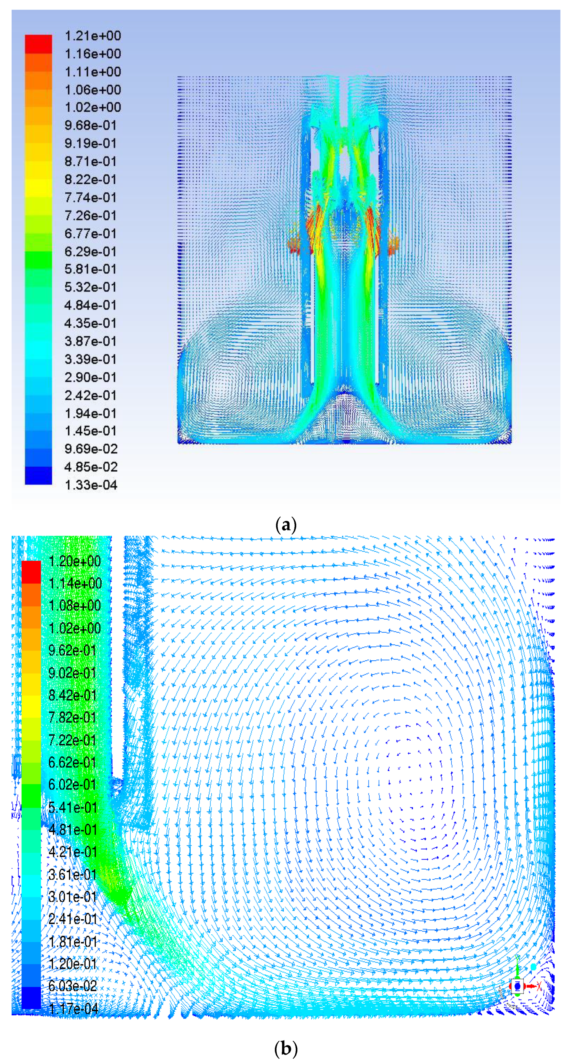
Figure 12.
Values of the mean Nusselt number for several Reynolds numbers obtained with MRF and Sliding Mesh approaches [22].
Figure 12.
Values of the mean Nusselt number for several Reynolds numbers obtained with MRF and Sliding Mesh approaches [22].
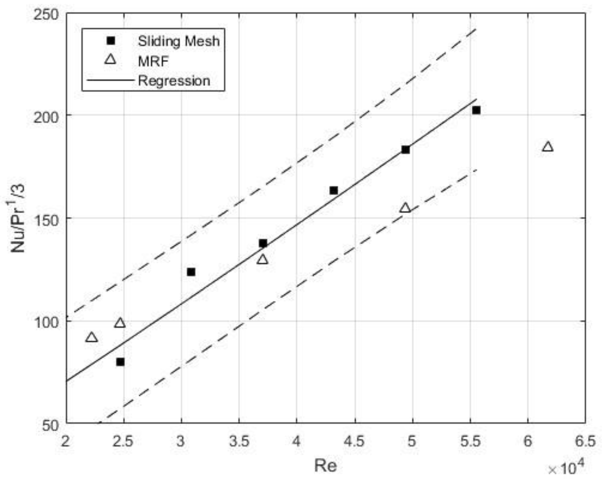

Table 1.
Data of the simulation at 500 RPM with different time steps [22].
Table 1.
Data of the simulation at 500 RPM with different time steps [22].
| Size of time step [sec] | 0.001 | 0.05 | 0.01 |
| Number of time steps | 20000 | 4000 | 2000 |
| Total wall-clock time [days] | 10.4 | 6.3 | 5.4 |
| Real time [days] | 15-17 | 8-10 | 4-6 |
| Total HTC [w/m2K] | 942.13 | 859.36 | 1066.41 |
| Total HTC extrapolated [w/m2K] | 1345.8 | ||
| GCI | 53.56 | 70.76 | 32.75 |
Table 2.
Values of the Nusselt and Reynolds numbers according to the rotational speed [22].
Table 2.
Values of the Nusselt and Reynolds numbers according to the rotational speed [22].
| Rotational speed [RPM] | Nusselt number | Re | ||
| Bottom | Wall | Total | ||
| 200 | 82.59 | 75.11 | 76.49 | 12344 |
| 300 | 108.39 | 75.83 | 81.85 | 18516 |
| 400 | 153.32 | 80.54 | 93.99 | 24688 |
| 500 | 236.31 | 99.04 | 124.4 | 30860 |
| 600 | 263.89 | 117.97 | 144.9 | 37032 |
| 700 | 311.93 | 142.11 | 173.5 | 43204 |
| 800 | 350.51 | 167.92 | 201.7 | 49376 |
| 900 | 387.26 | 191.27 | 227.5 | 55548 |
Table 3.
Values of the coefficients for the correlation of the Nusselt number [22].
Table 3.
Values of the coefficients for the correlation of the Nusselt number [22].
| c | Confidence interval for | m | Confidence interval for | |
| c | m | |||
| Bottom | 0.002 | -0.001 - 0.005 | 1.059 | 0.903 - 1.215 |
| Wall | 0.01 | -0.001 - 0.005 | 0.837 | 0.561 - 1.114 |
| Total | 0.005 | -0.001 - 0.005 | 0.913 | 0.723 - 1.104 |
Table 4.
Values of the coefficient for the second correlation of the Nusselt number (the exponent of the Reynolds number used was 0.8) [22].
Table 4.
Values of the coefficient for the second correlation of the Nusselt number (the exponent of the Reynolds number used was 0.8) [22].
| c | Confident interval for c | |
| Bottom | 0.030 | 0.028 - 0.033 |
| Wall | 0.014 | 0.013 - 0.016 |
| Total | 0.017 | 0.016 - 0.019 |
Table 5.
Values of the Nusselt number according to the mixing time, extrapolated values of the Nusselt number, and GCI at the bottom, wall, and the total [22].
Table 5.
Values of the Nusselt number according to the mixing time, extrapolated values of the Nusselt number, and GCI at the bottom, wall, and the total [22].
| BOTTOM (Nu-extrapolated = 221.09) | ||
| Mixing time | Nusselt | GCI |
| 20 | 236.31 | 8% |
| 30 | 232.36 | 6% |
| 40 | 225.9 | 2.60% |
| WALL (Nu-extrapolated = 89.52) | ||
| Mixing time | Nusselt | GCI |
| 20 | 99.04 | 12% |
| 30 | 96.06 | 8.50% |
| 40 | 93.84 | 5.74% |
| TOTAL (Nu-extrapolated = 103.43) | ||
| Mixing time | Nussel t | GCI |
| 20 | 124.41 | 21.07% |
| 30 | 121.25 | 18.36% |
| 40 | 118.25 | 15.65% |
Disclaimer/Publisher’s Note: The statements, opinions and data contained in all publications are solely those of the individual author(s) and contributor(s) and not of MDPI and/or the editor(s). MDPI and/or the editor(s) disclaim responsibility for any injury to people or property resulting from any ideas, methods, instructions or products referred to in the content. |
© 2024 by the authors. Licensee MDPI, Basel, Switzerland. This article is an open access article distributed under the terms and conditions of the Creative Commons Attribution (CC BY) license (https://creativecommons.org/licenses/by/4.0/).
Copyright: This open access article is published under a Creative Commons CC BY 4.0 license, which permit the free download, distribution, and reuse, provided that the author and preprint are cited in any reuse.


