
Submitted:
08 July 2024
Posted:
08 July 2024
You are already at the latest version
Abstract
(1) Background: Depressional wetlands are highly vulnerable to changes in temperature and rainfall, affecting littoral vegetation, thus HydroGeoMorphic (HGM) wetland types. This study aimed to assess the utility of Sentinel-2A vegetation indices in enhancing delineation and sub-classify depressional HGM types. (2) Methods: We sampled 84 pairs of four vegetation indices from 10x10m plots along 14 belt transects in eight depressional wetlands in Mpumalanga, South Africa. We evaluated vegetation index differences between and within wetlands, focusing on lit-toral gradients. (3) Results: Significant differences (Bonferroni p
Keywords:
Aichi Target 11
; Sentinel-2A
; Remote Sensing Vegetation Indices
; Salinity
; NDSI
; NDVI
; NDWI
; RENDVI
; Sustainable Development Goal (SDG) 6.6 & 15.1
1. Introduction
Wetland littoral vegetation and biodiversity are
crucial for wetland ecosystem services (McInnes, 2013; Pantshwa and Buschke,
2019). Water filtration, sediment trapping, floodwater retention, and carbon
storage are ecosystem services owed to wetland littoral vegetation (Krasnostein
and Oldham, 2004). Hence, wetlands have international importance (Goodwin,
2017; McInnes, 2013). They play an integral role in the ecology of the
watersheds where they are located and supply ecosystem services beyond the
boundaries of their watersheds (Laidig and Zampella, 1999; McKinney and
Charpentier, 2009). Many faunal and floral species of commercial importance,
such as fish, reeds and papyrus, are harvested from wetlands (Mnaya et al.,
2007; Rosenberger and Chapman, 1999; Zolfaghari, 2018). Wetlands are a wildlife
refuge and nursery. They are biodiversity hotspots and among the most
productive ecosystems worldwide (Lofgren, 2020; Pantshwa and Buschke, 2019; Wu
et al., 2018). Wetlands also control the amount and distribution of sediment
and nutrients. Hence, they influence floral and faunal organisms' temporal and
spatial distribution (Bird et al., 2014; Ngqulana et al., 2010). Wetlands
mitigate climate change through wetland carbon sequestration that outweighs its
methane (CH4) emissions despite being Earth's largest natural source of
185±21TgCyr1 atmospheric flux (Melton et al., 2013; Saunois et al., 2016; Zhu
et al., 2015). Wetlands have a low decomposition rate; hence they are estimated
to store 4% to 30% of Earth's 2500Pg soil C pool (Ji et al., 2020). Therefore,
human activity, i.e. drainage, overgrazing and vegetation change, needs to be
monitored. We have to safeguard the sequestration capacity of wetlands, prevent
biodiversity loss and increase carbon and methane emissions. However, the
limited use of wetland vegetation in wetland classification and delineation
methodology undermines the potential of wetland vegetation as an early-warning
indicator of wetland degradation.
Wetland vegetation is critical for wetland
biophysical processes responsible for the sustainability of wetland ecosystem
services (Dabrowska-Zielinska et al., 2014; Zheng et al., 2019). Without
properly functioning biophysical processes, wetlands would be unable to provide
the valuable ecosystem services they are popular for (Adekola et al., 2015;
Maltby and Acreman, 2011). Tall reeds found along the fringes reduce the speed
of water currents (Sieben et al., 2016). Reduction in water currents increases sand
and sediment deposition, which improves water quality (Fennessy et al., 1994;
Geng et al., 2021). During water drawdown, vegetation along the sandbank traps
floating chemicals and pathogens, exposing them to radiation (Salmon et al.,
2022). This trapping action allows the sun's radiation to sterilise pathogens
from the water. Adapted annual vegetation covers the sandbank during the winter
months, thus limiting excessive drying of the soil (Chirol et al., 2021).
Hence, healthy wetland vegetation is crucial for the sustainability of
depressional wetlands (Milaneschi et al., 2021). The loss of wetlands has
gained considerable attention over the past few decades, with over 50% loss
reported since 1900 (Davidson, 2014). That is why wetland monitoring under changing
climatic conditions focuses on the wetland littoral vegetation, which can be an
early warning proxy for changes in hydrology, soil chemistry and biodiversity.
Climate change threatens the persistence of
vegetation species along wetland littoral zones (Cao et al., 2020; Sieben et
al., 2021). Monitoring depressional wetlands at the national scale requires
more than qualitative ecological survey methods (Adam et al., 2010; Ovaskainen
et al., 2016; Thamaga et al., 2021). Meanwhile, remote sensing has become a
popular option for monitoring and mapping wetlands at national scale (Adam et
al., 2010; Adeli et al., 2020; Mahdavi et al., 2018). However, regarding vegetation
on the littoral banks of depressional wetlands, remote sensing data with
spatial scales that are small enough to quantify spatial changes in every meter
are still not freely available, e.g. World View and aerial images (Aroma and
Raimond, 2015; Baetz, 2000). Optical remote sensing is one of the most
attractive options because it offers vegetation indices, and some data are
distributed free of charge (Alam et al., 2021; Huete, 2012; Jackson and Huete,
1991; Verrelst et al., 2015). The opportunities to obtain optical remote
sensing data have improved due to the Sentinel-2A satellite launch on June 23,
2015 (Djamai et al., 2019). Now, it is collecting multispectral data, including
13 bands covering the visible, shortwave infrared bands (SWIR) wavelength regions
that are freely available (Huang et al., 2016). However, sufficient
consideration has not been given to the potential of Sentinel-2A vegetation
indices in quantifying the wetland boundary at 10m spatial resolution.
Sentinel-2A provides various vegetation spectral indices that can be extracted,
including the SWIR region (Sonobe et al., 2018). Plant properties influence
these indices, i.e. pigments, leaf water contents, biochemical, physiological
and biophysical properties that vary at resolutions <1m (Cho et al., 2008;
Main et al., 2011). There is interest in studying wetland vegetation using
remote sensing vegetation indices (Fernández-Manso et al., 2016; Pettorelli,
2013). NDVI values <0.20 represent non-vegetative surfaces, while values
<-0.0 represent water or very moist surfaces. However, NDVI values between
-0.0 and -0.4 and corresponding ranges in RENDVI, NDWI and NDSI have not been
declared or tested for the possibility of delaminating the wetland threshold.
We hypothesised that the detection of the wetland boundary could be achieved
using Sentinel-2A VIs, i.e. NDVI, RENDVI, NDWI and NDSI.
Literature on remote sensing vegetation indices
mainly focuses on vegetation classification or estimating vegetation
properties. Vegetation properties may include biomass (AGB) and leaf area index
(LAI). Literature that uses vegetation indices to study vegetation properties
such as wetland functional traits is rare. Similarly, literature that uses
vegetation indices to delineate and classify wetlands is uncommon. The
objectives of most studies in the literature on vegetation indices are often to
compare the performance of classification algorithms across acquisition dates
or data sources. Classification algorithms may include machine-learning, e.g.
k-nearest neighbours vs random forest vs support vector machines (Akbari et
al., 2021; Liu et al., 2018; Mutanga et al., 2012). Data sources may include
SPOT, Rapid Eye, Landsat and MODIS, while Sentinel 2 is less covered.
Sentinel-2A provides the red-edge spectral bands that extend its potential
usefulness for analysis of wetland vegetation, but free of charge and at the
competitive spatial resolution, i.e. ten vs 20m compared to 30m or greater
(Koutsias and Pleniou, 2015). The sampling of training data is often completed
through random selection of field plots. However, research questions require
gradient analysis over a small scale, e.g. 10 m. Hence purposeful sampling at
10m spatial resolution is preferred and ensures that the researcher understands
the sampling effects and their impact on the delineation and classification
results while avoiding data contamination.
Due to the reasons outlined above, it is
justifiable to investigate the feasibility of delimiting and classifying
depression wetlands using Sentinel-2A Vegetation Indices (VIs). The use of
gradient analyses and parametric statistics of remote sensing data derived from
systematic transect sampling; is novel and justifiable. To our knowledge,
Sentinel-2A data have not been used to estimate the threshold between wetland
and dryland before. Based on the experience of other researchers who
investigated a variety of satellite sensors in wetland vegetation, we see
Sentinel-2A images as a valuable source of data for such applications. In the
context of VIs in wetlands, studies that do not use machine-learning or mapping
methods are also limited. Within this framework, the present study aimed to
evaluate the potential of Sentinel-2A data for delineating the wetland
threshold and classifying wetlands. The objectives were (i) to assess
differences in Sentinel-2A vegetation indices between wetlands for
classification (ii) to analyse trends of Sentinel-2A vegetation indices from
the open waterbody to the outer dryland to assess the presence of an inflexion
point between dryland and wetland.
2. Materials and Methods
General Methodology
The study was conducted systematically, and all the
critical steps were recorded to ensure repeatability. The general methodology (Figure 1) includes satellite remote sensing
data, which was used to guide the process of selecting sample plots, transects,
wetland sites and ecological and data science principles. The alignment of the
data collection with remote sensing ancillary data ensured further
repeatability because remote sensing data is publicly available. Therefore, the
exact sample locations where these data were collected can be retrieved by
subsequent researchers.
Selection of Study Area
The Mpumalanga Lake District (MLD) was chosen as a
study area because it has a rich diversity of depressions (and other wetlands).
MLD is a good case study for isolated wetland ecosystems globally like the
Prairie Pothole Region (PPR) in the northern Great Plains of the US. A sequence
of two strata underlies the geology of MLD. In the stratigraphic order of
stratigraphy, the Ecca Group is first; dominated by sedimentary deposits
composed chiefly of shale and sandstone, followed by the Dwyka Group below it
(Smith et al., 1993). The Dwyka Group primarily consists of diamictite,
tillite, claystone, mudstone and sometimes quartzite or sandstone shale
(Visser, 1986). The catchment receives 767 mm of mean annual precipitation
(Nondlazi et al., 2021). Catchment W55A has over 300 depressional wetlands in
just a 20-odd kilometre radius (Nondlazi et al., 2021). Within MLD, a subset of
depressional wetlands was selected (, Lake Banagher Farm, 26°20'11.21 "S,
30°21'14.03 "E, in the Gert Sibande District, in the Msukaligwa Local
Municipality, Mpumalanga Province, South Africa. The wetland (ecosystem types
and vegetation). The diversity is due to variations in elevation, size, shape
and width of the vegetated littoral zones. Therefore, sampling the MLD presents
a good chance of covering a wide range of depressional wetland habitats in a
relatively small area.
Selection of Sampling Locations the Depressional Wetland Sites
Eight depressional wetlands were selected to
represent the range of depressional habitats (Figure 2). The diversity of wetlands was observed in terms of (a) extent of the
waterbody, (b) extent of vegetation cover, (c) shape and (d) size.
Research manuscripts reporting large datasets that
are deposited in a publicly available database should specify where the data
have been deposited and provide the relevant accession numbers. If the
accession numbers have not yet been obtained at the time of submission, please
state that they will be provided during review. They must be provided prior to
publication.
Interventionary studies involving animals or
humans, and other studies that require ethical approval, must list the
authority that provided approval and the corresponding ethical approval code.
Field Surveys Design
Two field surveys were conducted to collect ground
truth data for wetland NDVI, RENDVI, NDSI and NDWI, i.e. Above Ground Biomass
(AGB), Plant Species Richness (PSR), Vegetation Moisture Content (VMC). The
first survey was conducted in March 2018, and the second was conducted in
November 2018. The first survey focused on two big (0.30-1.3km2) wetlands, and
the second focused on six smaller (0.003k-0.22km2) wetlands. Only two wetlands
had data collected in both sampling periods. The repeated wetlands were used to
quantify and ensure that the change in vegetation growth was negligible between
the two sampling periods. The sampling procedure was based on the belt
transect method according to the Sentinel-2A pixels scheme. Sentinel-2A
provides data with global coverage in a five-day revisit cycle side, making an
overpass from above the equator. In addition to near-infrared and shortwave
infrared bands, it has three red-edge bands (Bands 5-7 (NIR) centre of the SWIR
at 705, 740 and 783 nm, respectively), which have been proven helpful in
vegetation classification. The intention was to cover the range of variation in
the visible vegetation physiognomy from the water's edge to the dryland area (Figure 3). The best location for transects was
the region of the wetland-dryland gradient that had the highest turnover in
pixel tone (colour variation). A high variation of pixel tone was considered to
reflect higher turnover in species or vegetation structure or both. At each
wetland, a field survey was conducted. The belt transect method was preferred
to adequately sample the longitudinal gradient from the waterbody to the
dryland. The width of the transects was 10m in line with the spatial resolution
of Sentinel-2A. Transects had varying lengths, dependent on the width of the
littoral zone being sampled (30m - 130 m).
Setting Up the Belt Transects
A mash grid made up of contiguous 10m plots was
generated in ArcGIS ArcMap 10.5. This grid was overlaid on a true colour
composite of the Sentinel-2A to identify the best locations for transects,
following the approach by Goodman (1990). For wetlands greater than 0.2 km2
(the three most extensive wetlands, Appendix C),
three transects were sampled around each wetland (Figure 2). For the smaller wetlands, one
transect was sampled. Plots with similar vegetation structure and composition
as the ones preceding them were not sampled to avoid repetition. Purposeful
sampling ensured that the sampling maximised the efficiency of a representative
sampling of landscape features and avoided repetitive sampling and anomalies,
e.g. termite mounds. The length of a transect was limited by the fence or by
reaching the dry ground.
Imagery Collection, Data Pre-Processing and Selecting Vegetation Indices
Concurrent availability of 10-day Sentinel-2A data
provides an unprecedented opportunity to gather high-resolution (10m) data for
national mapping of wetland ecosystems. Sentinel-2A data became available for
South Africa in the middle of 2015, and its capabilities to map wetland
ecosystem types, boundaries and species still require adequate assessment. The
easy and simultaneous access to the entire archive of Sentinel-2A products
through fast and scalable computational machine learning tools. Google Earth Engine
(GEE) makes machine learning an essential and powerful tool for wetland
monitoring and assessment. Processing cloud-free imagery can be computationally
challenging. However, the combined use of coding computations in R and GEE
offers seamless alternatives to expensive software such as ArcGIS and
ENvironmet for Visualising Images (ENVI).
The study location (Lake Banagher farm) was
identified and delineated with a polygon using six/seven vertices. A
Sentinel-2A Multispectral Instrument (MSI), Level-2A image collection was
downloaded from the European Union - Copernicus (ESA). Images that fall within
the interval of the target dates ("2017-07-01",
"2020-09-30") were filtered and downloaded from the Sentinel-2A
collection of images using the "filterDate" function algorithm. The
resulting subset collection was sorted into ascending cloud cover (from the
least cloud cover to the highest) using the "sort" function. This
function uses the Sentinel-2A cloud probability from the Sentinel-2A cloud
detector library (using "LightGBM"). All bands were up-scaled through
resampling using bilinear interpolation to 10m resolution before applying the
"gradient boost base" algorithm. The resulting 0 to 1 floating point
probability is scaled as 0 to 100 and stored as a UINT8. Areas missing any or
all of the bands were masked out. Higher values are considered to be clouds or
highly reflective surfaces. The first image out of this collection - i.e. the
most cloud-free image was selected and used for the analysis (COPERNICUS/S2
SR/20191004T074749 20191004T080733 T36JTR). Define visualisation parameters
were de ned in a JavaScript dictionary to render a true colour composite as
bands 4,3 and 2 as RGB, respectively. Normalised Different Salinity Index
(NDSI) was computed as" (SWIR1 - SWIR2) / (SWIR1 + SWIR2)". Where
SWIR1="B11" (1610 nm) and SWIR2 = "B12" (2190 nm) at a
spatial resolution of 20 m. Normalised Difference Water Index (NDWI) was
computed as" (GREEN - NIR) / (GREEN + NIR)". Where
GREEN="B03" (560 nm) and NIR= "B08" (842 nm) at a spatial
resolution of 10 m. Normalised Difference Vegetation Index (NDVI) was computed
as" (NIR - Red) / (NIR + Red)". Where NIR="B08" (842 nm)
and Red= "B04" (665 nm) at a spatial resolution of 10 m. Red-edge
Normalised Difference Vegetation Index (RENDVI) was computed as" (VRE1 -
VRE2) / (VRE1 + VRE2)". Where VRE1="B05" (705 nm) and VRE2=
"B06" (740 nm) at a spatial resolution of 20m (Figure 3).
Normalised Difference (NDVI) and Red-Edge Normalised Difference Vegetation Index (RENDVI)
The normalised difference vegetation index (NDVI)
was one of the first satellite vegetation indices and strongly correlates with
canopy cover (r2 = 0.84), photosynthesis and primary production of vegetation
(Cho and Ramoelo, 2019). Sentinel-2A NDVI was calculated using the visible red
(VisRed) and the Near Infrared (NIR) bands. These regions are often used to
analyse vegetation (Kaplan and Avdan, 2017). These regions interact with
vegetation tissues' internal pigment and chemistry. The red-edge NDVI is less
prone to saturation because it penetrates the vegetation canopy. This ability
to penetrate means measuring the variation of leaf foliage that is not exposed,
located at the bottom of the canopy. Meanwhile, NDVI declines when the species
composition changes to more sedge species because of fewer leaves and,
therefore, less chlorophyll among sedge species. While this decline in NDVI
could confound the decline in NDVI that is a response to the decrease in
vegetation biomass, it might be useful for detecting an increase in the
abundance of sedge species along the littoral gradient of wetlands.
Normalised Difference Salinity Index (NDSI)
The natural interaction between salty seawater and
soils along the coastline has driven the wide application of remote sensing
indices of soil salinity (Abdel-Kader, 2013; Chi et al., 2019; Das et al.,
2011). Monitoring salinity intrusion has been a key application area for soil
salinity indices (Nguyen et al., 2020). The normalised different salinity index
(NDSI) accurately detects overall salinity and applies to exposed soils
(Al-Khaier, 2003). The application of the salinity index to detect changes in
soil chemical salt conditions has been widely used in the literature despite
the limitation where vegetation covers the soil. The idea of collecting soil
samples underneath vegetation over a geo-referenced spatial scale and analysing
it using laboratory spectroscopy can solve the challenge of vegetation cover
but has not been widely tested. Variations in the salt content of the soil
underneath vegetation pose another unique challenge when correcting soil
background attenuation with vegetation cover.
Normalised Difference Water Index (NDWI)
The Normalised Difference Water Index (NDWI) is
derived from a band ratio of Near-Infrared (NIR) and Short Wave Infrared (SWIR)
channels (Gao, 1996, 1995). The traditional application, such as that of Tucker
(1980), emanates from the premise of the response of SWIR reflectance to
changes in both the vegetation water content and abundance of spongy mesophyll
cell structure in vegetation canopies. The response of the NIR reflectance to
leaf internal structure and leaf dry matter content (Ceccato et al., 2002,
2001; Huang et al., 2018; Jackson et al., 2004) can be helpful. For example,
the abundance of mesophyll cells signifies the abundance of obligate wetland
vegetation. Against this background, we hypothesised the non-traditional use of
dry soil samples (Delbart et al., 2005). We hypothesise that these two
wavelength regions (SWIR and NIR) should also respond to variations in soil
structure. Gu et al. (2008) proposed that its response to the structures of
spongy mesophyll cells would also interact with the different soil structural
compositions that emanate from differences in waterlogging characteristics of
soil along the wetland gradient (Delbart et al., 2005; Jackson et al., 2004).
3. Data Analysis
Density plots and box and whiskers plots were used
to visualise and assess the variability of the three vegetation remote sensing
indices. Significance tests were conducted to assess the statistical validity
of the results. All analyses were conducted using R version 3.6.2 (R
Development Core Team, 2019). The Tukey Honest Significant Difference test,
accounting for the Bonferroni effect, controlled Type I errors in multiple
comparisons. To test the significance of the hypotheses at = 0.05, the possible
number of combinations or Bonferroni coefficient (m) for eight wetlands was
m=28. The "m" value and a new alpha level of 0.001 were calculated
using the combination formula (Equation (5)). Where the default alpha level
(0.05) is divided by “m” i.e. (nCr = n / r * (n - r)). Where n represents the
total number of items, i.e. 8, and "r" represents the number of items
being compared at a time, i.e. 2, to calculate the Bonferroni adjustment alpha
level. Maps in this paper were created using ArcGIS® and ArcMap® software by
Esri; used herein under intellectual property license, Copyright Esri©, unless
otherwise stated. For more information about Esri® software, please visit
www.esri.com.
4. Results
The mean NDVI values (Figure 4) of the eight wetlands were significantly different (F 7;77 = 4.3539, p< 0.001) at Bonferroni adjusted alpha level (p<0.001, One-way ANOVA) and NDSI (F 7;77= 7.0765, p< 0.001) but not NDWI (F 7;77= 3.135, p=0.0058), RENDVI (F 7;77 = 3.1995, p=0.005). The results from ordination analysis, conducted using all four variables, revealed three groups of wetlands (Principal Component Analysis (PCA)). Group A biased towards NDVI and NDSI, group B is biased towards NDWI and group C is biased towards RENDVI. The first two PCA axes were the most important latent variables that correlated (88.38%) to the four variables. The first PCS axis was biased toward RENDVI (18.78%), and the second PCA axis was biased towards NDWI (69. 51%). Therefore, based on the eigenvalues of the correlation matrix for the four active variables, ordination results further support the ANOVA findings of the importance of spectral difference in differentiating the wetlands from one another (Figure 5).
Trends of Edaphic Factors Along the Wetland Gradient
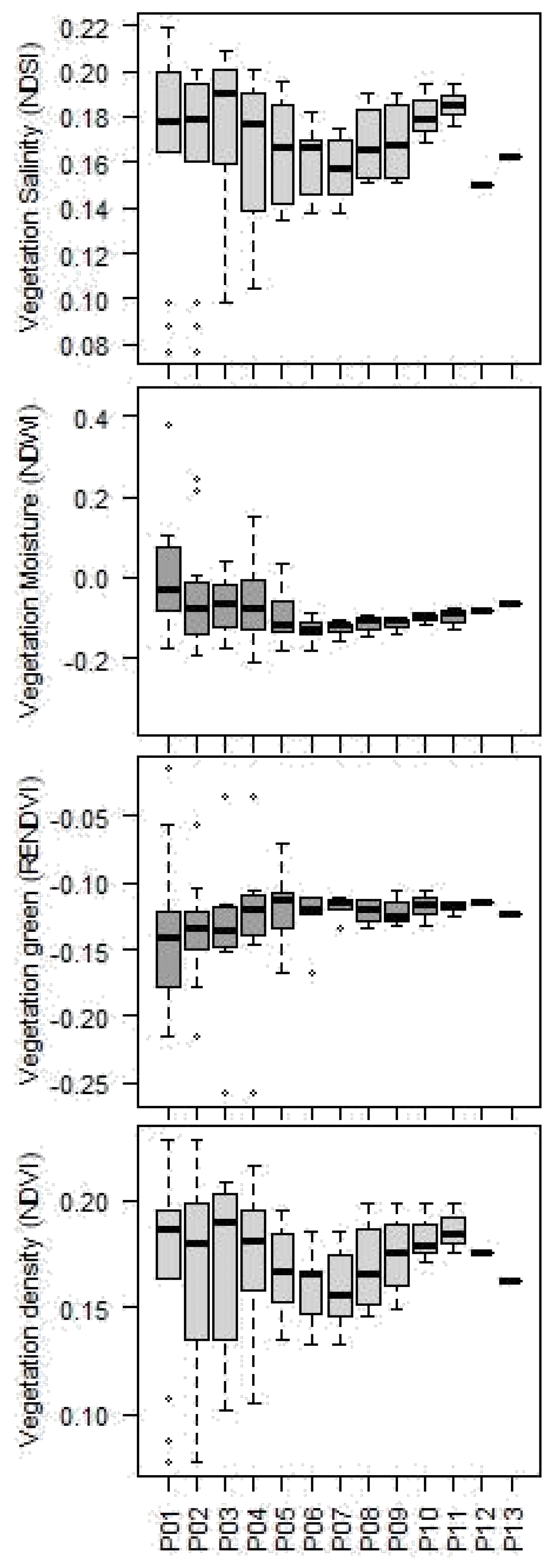
Generally, there were negative trends in the response of NDSI (r2=0.96-0.34), NDVI (r2=0.99-0.20) and NDWI (r2=0.95-0.20) along the gradient from the centres of the wetlands to the outer dryland boundary, while RENDVI had positive trends (r2=0.95-0.25). However, at relatively short distances, ranging from 30 to 70 m. This distance probably reflected the extent of the palustrine section of the depressional wetlands (Figure 6). When the data from the remote sensing indices were combined across the gradients of all wetlands to drylands, the index maintained their general trends, NDSI, NDVI and NDWI = negative, and RENDVI = positive (Figure 7). The change of the patterns of Sentinel-2A indices, which probably reflects the mean seasonal maximum extent of the wetland, at 70m on average for combined data with the 8th plot (80 m) showing a change in the direction of the pattern to the opposite direction.
5. Discussion
Differences in remote sensing vegetation indices across the depressional wetland
This study investigated differences in selected remote sensing indices of vegetation among eight depressional wetlands in a temperate grassland biome. Our results showed that significant (p<0.001) site-level differences were detected for two of the indices, NDVI (1/28) and NDSI (1/28), between wetland pairs. Four other wetlands showed a significant difference at p<0.05. Wilson and Norman (2018) analysed spatial and temporal trends in vegetation greenness and soil moisture. Still, they used normalised difference infrared index (NDII) instead of normalised difference water index NDWI and normalised difference vegetation index (NDVI) from Landsat instead of Sentinel-2A. To our knowledge, vegetation indices derived from Sentinel-2A data have not been used to estimate the thresholds between wetland and dryland or to delineate wetlands or group wetland sites in the MLD (Wilson and Norman, 2018). Wilson and Norman also noted the effect of grazing on canopy cover (2018), lowered NDVI performance, while NDII was better at tracking changes in areas with continuous grazing. Results from Wilson and Norman (2018) could explain why only one out of 28 pairs was significantly different as all the other camps where the other wetlands are found were grazed. Lumipan was in a rested camp, to be grazed following Blinkpan, which was being fed during the time of sampling. These results can be relied upon because they were produced with data collected from cloud-free images (<5% cloud cover), and the indices were manually calculated using a javascript in GEE. This use of GEE and cloud-free images means that the image quality, location reference and calculations were based on a standard protocol collected together with management information and are repeatable. There is a need for further research on the seasonal time-series of vegetation spectral indices of depressional wetlands (Li et al., 2017). We tested similarities in spectral indices across the wetland sites. The differences in spectral indices across the eight wetlands showed that although the wetlands differ in characteristics that partly affect or drive the spectral indices, there is still high convergence or grouping in the trends of vegetation spectral indices. The meaning similarity in spectral indices is present within formed groups. These groups are more likely to result in wetland groups with similar functioning. Two wetlands were distinct from each other (Blinkpan and Slangpan), while other wetlands were similar.
Patterns of Remote Sensing Vegetation Indices Along the Wetland Littoral Gradient
The trends in vegetation spectral indices are related to field capacity and edaphic factors, including the amount of water content held in the soil after excess water has drained away and the rate of downward movement has decreased (Castelli et al., 2000; Colman, 1947; Twarakavi and Sakai, 2009). Furthermore, NDVI can be strongly influenced by surface and groundwater availability (Aguilar et al., 2012; Fu and Burgher, 2015). The available water capacity is also crucial in explaining these patterns. It refers to the ability of soil to hold water from infiltrating to the lower levels of the soil profile yet make it available to plants (Cassel and Nielsen, 1986). It is the water held between field capacity and the wilting point.
The wetland-dryland threshold boundary for delineating endorheic wetlands
In this research, we tested whether remote sensing vegetation indices can be used to delineate the boundary of endorheic wetlands by thresholding wetland edaphic factors, similar to studies in the PPR, situated in the temperate grasslands of the US (Wu and Lane, 2016). However, the delineation of thresholds of endorheic wetlands from Wu and Lane (2016) is based on a micro elevation determined using Light Detection and Ranging. It does not specify the distance from the wetland waterbody. In this study, the empirically derived threshold of the maximum extent of individual wetlands ranged between 30m and 70 m. However, the aggregate threshold for all eight depressional wetlands, based on the three median vegetation remote sensing indices, was 70 m. Hence, we recommend using a maximum buffer of 100m to add a precautionary vegetation buffer of 30m to accommodate the ferralitic zone of incoming subsurface seepage. The buffer width should be based on site-specific recommendation using the percentage change threshold; hence the 100m is a policy recommendation, not a scientific result. Ma (2016) suggests a minimum buffer of 20m (Semlitsch and Bodie, 2003). Wetland buffering is vital for wetland management and water protection, flooding control, groundwater storage, habitat for wild species, recreation, aesthetics and removal of sediment and pollutants (Castelle and Johnson, 1994; Correll, 1996; Gleason et al., 2003; Wenger and Fowler, 2000). In theory, a generalisation of a percentage change threshold can be used in the place of a distance measure. This theoretical approach allows the results of our study to be applied to other wetlands globally and can therefore be theoretically represented (Equation (6)) for determining the wetland threshold using empirical measurements of edaphic factors (Nondlazi et al., 2021). Therefore, this result is crucial for the South African policy framework and environmental impact assessments (Sandham et al., 2019).
6. Conclusions
Study results showed that depressional wetlands of the temperate grassland biome differ significantly in remote sensing indices. There are correlations between these remote sensing vegetation indices and field measurements at the plot or pixel level, but the regression relationships remain tested. However, similarities are present among some of the wetlands depressions are related to the size of the littoral zones. This study also revealed consistent horizontal trends in the vegetation remote sensing indices from the open water to the outer dryland characterised.This study also revealed consistent horizontal trends in the vegetation remote sensing indices from the open water to the outer dryland, characterised by a declining trend for NDSI, NDVI, NDWI and increasing trends for RENDVI. This study demonstrated that for depression wetlands within the MLD, the wetland threshold (threshold between dryland and wetland) could be empirically detected at a relatively short distance of about 30 to 70 metres; a threshold where the trends of vegetation remote sensing indices change to opposite directions with a percentage change that is greater than 5%. This threshold can potentially inform the delineation of the outer edge of endorheic wetlands, which are poorly mapped globally for under threat wetlands.
Author Contributions
Basanda Xhantilomzi Nondlazi - BN: PhD candidate - Prepared proposal, collected data, Analysed, Wrote the manuscript, data capture, data quality and methods validation in the field. Moses Azong Cho - MC: Main supervisor - Supervised preparation of the proposal, technical planning of fieldwork, data capture and quality, analysis, and manuscript writing. Heidi van Deventer - HD: The second supervisor - Supervised preparation of the proposal, financial planning of fieldwork, analysis, and manuscript writing. Erwin Jacobus Sieben - ES: University supervisor - Supervised preparation of the proposal, fieldwork collection of data, analysis and writing of the manuscript. Data quality and methods validation in the field.
Funding
This work was funded by the South African Water Research Commission (WRC), under the project K5/2545 'Establishing remote-sensing tool-kits for monitoring freshwater ecosystems under global change, the National Research Foundation (NRF) PhD Professional Development Programme, as well as the Council for Scientific and Industrial Research (CSIR) Smart Places bursary 2020 and the University of KwaZulu-Natal (UKN) Postgraduate fees remission programme.
Consent for Publication
The consent for publication was obtained following the internal procedures at the host institutions and from funders.
Ethics
To the best of their knowledge, the authors have identified no conflict of interest. The Council approved the publication of this manuscript for Scientific and Industrial Research (CSIR). The agreements for publication considers ethics, including patenting considerations at the time of the publication. However, the study did not include animal or human subjects.
Data Availability Statement
The data can be accessed.
Acknowledgments
This work was funded by several institutions, including the Council for Scientific and Industrial Research; Water Research Commission (WRC) under project K5/2545, titled ‘Establishing Remote Sensing Toolkits for Monitoring freshwater ecosystems under global change’; the University of KwaZulu-Natal and the Professional Development Programme (PDP) of South Africa’s National Research Foundation.We also thank Mr Prince Malomane, the owner of Lake Banagher Farm, for allowing access to the sites and his hospitality and that of his farm workers, who also assisted with collecting some of the samples.
Conflicts of Interest
We declare we have no competing interests.
References
- Abdel-Kader, F.H., 2013. Digital Soil Mapping Using Spectral and Terrain Parameters and Statistical Modelling Integrated into GIS-Northwestern Coastal Region of Egypt, in: Shahid, S.A., Taha, F.K., Abdelfattah, M.A. (Eds.), Developments in Soil Classification, Land Use Planning and Policy Implications: Innovative Thinking of Soil Inventory for Land Use Planning and Management of Land Resources. Springer Netherlands, Dordrecht, pp. 353–371.
- Adam, E.; Mutanga, O.; Rugege, D. Multispectral and hyperspectral remote sensing for identification and mapping of wetland vegetation: a review. Wetl. Ecol. Manag. 2009, 18, 281–296. [Google Scholar] [CrossRef]
- Adekola, O.; Mitchell, G.; Grainger, A. Inequality and ecosystem services: The value and social distribution of Niger Delta wetland services. Ecosyst. Serv. 2015, 12, 42–54. [Google Scholar] [CrossRef]
- Adeli, S.; Salehi, B.; Mahdianpari, M.; Quackenbush, L.J.; Brisco, B.; Tamiminia, H.; Shaw, S. Wetland Monitoring Using SAR Data: A Meta-Analysis and Comprehensive Review. Remote. Sens. 2020, 12, 2190. [Google Scholar] [CrossRef]
- Aguilar, C.; Zinnert, J.C.; Polo, M.J.; Young, D.R. NDVI as an indicator for changes in water availability to woody vegetation. Ecol. Indic. 2012, 23, 290–300. [Google Scholar] [CrossRef]
- Akbari, V.; Simpson, M.; Maharaj, S.; Marino, A.; Bhowmik, D.; Prabhu, G.N.; Rupavatharam, S.; Datta, A.; Kleczkowski, A.; Sujeetha, J.A.R.P. Monitoring Aquatic Weeds in Indian Wetlands Using Multitemporal Remote Sensing Data with Machine Learning Techniques. IGARSS 2021 - 2021 IEEE International Geoscience and Remote Sensing Symposium. LOCATION OF CONFERENCE, BelgiumDATE OF CONFERENCE; pp. 6847–6850.
- Alam, M.; Wang, J.-F.; Guangpei, C.; Yunrong, L.; Chen, Y. Convolutional Neural Network for the Semantic Segmentation of Remote Sensing Images. Mob. Networks Appl. 2021, 26, 200–215. [Google Scholar] [CrossRef]
- Al-Khaier, F., 2003. Soil Salinity Detection Using Satellite Remote Sensing. ITC.
- Aroma, R.J., Raimond, K., 2015. A review on availability of remote sensing data, in: 2015 IEEE Technological Innovation in ICT for Agriculture and Rural Development (TIAR). ieeexplore.ieee.org, pp. 150–155.
- Baetz, W., 2000. Availability of Current Spaceborne Earth Observation Data, in: Buchroithner, M.F. (Ed.), Remote Sensing for Environmental Data in Albania: A Strategy for Integrated Management. Springer Netherlands, Dordrecht, pp. 31–40.
- Bird, M.S.; Day, J.A.; Malan, H.L. The influence of biotope on invertebrate assemblages in lentic environments: A study of two perennial alkaline wetlands in the Western Cape, South Africa. Limnologica 2014, 48, 16–27. [Google Scholar] [CrossRef]
- Cao, B.; Bai, C.; Xue, Y.; Yang, J.; Gao, P.; Liang, H.; Zhang, L.; Che, L.; Wang, J.; Xu, J.; et al. Wetlands rise and fall: Six endangered wetland species showed different patterns of habitat shift under future climate change. Sci. Total. Environ. 2020, 731, 138518. [Google Scholar] [CrossRef] [PubMed]
- Cassel, D.K., Nielsen, D.R., 1986. Field capacity and available water capacity. Methods of Soil Analysis: Part 1 Physical and Mineralogical Methods 5, 901–926.
- Castelle, A.J.; Johnson, A.W.; Conolly, C. Wetland and Stream Buffer Size Requirements—A Review. J. Environ. Qual. 1994, 23, 878–882. [Google Scholar] [CrossRef] [PubMed]
- Castelli, R.M.; Chambers, J.C.; Tausch, R.J. Soil-plant relations along a soil-water gradient in great basin riparian meadows. Wetlands 2000, 20, 251–266. [Google Scholar] [CrossRef]
- Ceccato, P.; Flasse, S.; Tarantola, S.; Jacquemoud, S.; Grégoire, J.-M. Detecting vegetation leaf water content using reflectance in the optical domain. Remote. Sens. Environ. 2001, 77, 22–33. [Google Scholar] [CrossRef]
- Ceccato, P.; Gobron, N.; Flasse, S.; Pinty, B.; Tarantola, S. Designing a spectral index to estimate vegetation water content from remote sensing data: Part 1. Remote. Sens. Environ. 2002, 82, 188–197. [Google Scholar] [CrossRef]
- Chirol, C.; Spencer, K.L.; Carr, S.J.; Möller, I.; Evans, B.; Lynch, J.; Brooks, H.; Royse, K.R. Effect of vegetation cover and sediment type on 3D subsurface structure and shear strength in saltmarshes. Earth Surf. Process. Landforms 2021, 46, 2279–2297. [Google Scholar] [CrossRef]
- Chi, Y.; Sun, J.; Liu, W.; Wang, J.; Zhao, M. Mapping coastal wetland soil salinity in different seasons using an improved comprehensive land surface factor system. Ecol. Indic. 2019, 107, 105517. [Google Scholar] [CrossRef]
- Cho, M.A.; Ramoelo, A. Optimal dates for assessing long-term changes in tree-cover in the semi-arid biomes of South Africa using MODIS NDVI time series (2001–2018). Int. J. Appl. Earth Obs. Geoinformation 2019, 81, 27–36. [Google Scholar] [CrossRef]
- Cho, M.A.; van Aardt, J.; Majeke, B.; Main, R. Evaluating the Seasonality of Remote Sensing Indicators of System State for Eucalyptus Grandis Growing on Different Site Qualities. IGARSS 2008 - 2008 IEEE International Geoscience and Remote Sensing Symposium. LOCATION OF CONFERENCE, United StatesDATE OF CONFERENCE; pp. III - 487–III - 490.
- Colman, E.A. A LABORATORY PROCDURE FOR DETERMINING THE FIELD CAPACITY OF SOILS. Soil Sci. 1947, 63, 277–284. [Google Scholar] [CrossRef]
- Correll, D.L., 1996. Buffer zones and water quality protection: General principles. Buffer zones: Their processes and potential in water protection 7–20.
- Dabrowska-Zielinska, K.; Budzynska, M.; Tomaszewska, M.; Bartold, M.; Gatkowska, M.; Malek, I.; Turlej, K.; Napiorkowska, M. Monitoring Wetlands Ecosystems Using ALOS PALSAR (L-Band, HV) Supplemented by Optical Data: A Case Study of Biebrza Wetlands in Northeast Poland. Remote. Sens. 2014, 6, 1605–1633. [Google Scholar] [CrossRef]
- Das, N.N.; Entekhabi, D.; Njoku, E.G. An Algorithm for Merging SMAP Radiometer and Radar Data for High-Resolution Soil-Moisture Retrieval. IEEE Trans. Geosci. Remote. Sens. 2010, 49, 1504–1512. [Google Scholar] [CrossRef]
- Davidson, N.C. How much wetland has the world lost? Long-term and recent trends in global wetland area. Mar. Freshw. Res. 2014, 65, 934–941. [Google Scholar] [CrossRef]
- Delbart, N., Kergoat, L., Le Toan, T., Lhermitte, J., Picard, G., 2005. Determination of phenological dates in boreal regions using normalised difference water index. Remote Sens. Environ. 97, 26–38.
- Djamai, N., Fernandes, R., Weiss, M., McNairn, H., Goïta, K., 2019. Validation of the Sentinel Simplified Level 2 Product Prototype Processor (SL2P) for mapping cropland biophysical variables using Sentinel-2/MSI and Landsat-8/OLI data. Remote Sens. Environ. 225, 416–430.
- Fennessy, M.S.; Brueske, C.C.; Mitsch, W.J. Sediment deposition patterns in restored freshwater wetlands using sediment traps. Ecol. Eng. 1994, 3, 409–428. [Google Scholar] [CrossRef]
- Fernández-Manso, A.; Fernández-Manso, O.; Quintano, C. SENTINEL-2A red-edge spectral indices suitability for discriminating burn severity. Int. J. Appl. Earth Obs. Geoinformation 2016, 50, 170–175. [Google Scholar] [CrossRef]
- Fu, B.; Burgher, I. Riparian vegetation NDVI dynamics and its relationship with climate, surface water and groundwater. J. Arid. Environ. 2015, 113, 59–68. [Google Scholar] [CrossRef]
- Gao, B.-C., 1996. NDWI—A normalised difference water index for remote sensing of vegetation liquid water from space. Remote Sens. Environ. 58, 257–266.
- Gao, B.C., 1995. Normalised difference water index for remote sensing of vegetation liquid water from space. Imaging Spectrometry.
- Geng, M.; Wang, K.; Yang, N.; Li, F.; Zou, Y.; Chen, X.; Deng, Z.; Xie, Y. Spatiotemporal water quality variations and their relationship with hydrological conditions in Dongting Lake after the operation of the Three Gorges Dam, China. J. Clean. Prod. 2020, 283, 124644. [Google Scholar] [CrossRef]
- Gleason, R.A.; Euliss, N.H.; Hubbard, D.E.; Duffy, W.G. Effects of sediment load on emergence of aquatic invertebrates and plants from wetland soil egg and seed banks. Wetlands 2003, 23, 26–34. [Google Scholar] [CrossRef]
- Goodwin, E.J., 2017. Convention on Wetlands of International Importance, especially as Waterfowl Habitat 1971 (Ramsar), in: Elgar Encyclopedia of Environmental Law. Edward Elgar Publishing Limited, pp. 101–108.
- Gu, Y.; Hunt, E.; Wardlow, B.; Basara, J.B.; Brown, J.F.; Verdin, J.P. Evaluation of MODIS NDVI and NDWI for vegetation drought monitoring using Oklahoma Mesonet soil moisture data. Geophys. Res. Lett. 2008, 35. [Google Scholar] [CrossRef]
- Huang, G.; Li, X.; Huang, C.; Liu, S.; Ma, Y.; Chen, H. Representativeness errors of point-scale ground-based solar radiation measurements in the validation of remote sensing products. Remote. Sens. Environ. 2016, 181, 198–206. [Google Scholar] [CrossRef]
- Huang, Y.B.; Chen, Z.-x.; Yu, T.; Huang, X.-z.; Gu, X.-f. Agricultural remote sensing big data: Management and applications. J. Integr. Agric. 2018, 17, 1915–1931. [Google Scholar] [CrossRef]
- Huete, A.R. Vegetation Indices, Remote Sensing and Forest Monitoring. Geogr. Compass 2012, 6, 513–532. [Google Scholar] [CrossRef]
- Jackson, R.D.; Huete, A.R. Interpreting vegetation indices. Prev. Veter- Med. 1991, 11, 185–200. [Google Scholar] [CrossRef]
- Jackson, T.J., Chen, D., Cosh, M., Li, F., Anderson, M., Walthall, C., Doriaswamy, P., Hunt, E.R., 2004. Vegetation water content mapping using Landsat data derived normalised difference water index for corn and soybeans. Remote Sens. Environ. 92, 475–482.
- Ji, H.; Han, J.; Xue, J.; Hatten, J.A.; Wang, M.; Guo, Y.; Li, P. Soil organic carbon pool and chemical composition under different types of land use in wetland: Implication for carbon sequestration in wetlands. Sci. Total. Environ. 2020, 716, 136996. [Google Scholar] [CrossRef]
- Kaplan, G.; Avdan, U. Mapping and Monitoring Wetlands Using Sentinel-2 Satellite Imagery. ISPRS Ann. Photogramm. Remote Sens. Spat. Inf. Sci. 2017, 4, 271–277. [Google Scholar] [CrossRef]
- Koutsias, N.; Pleniou, M. Comparing the spectral signal of burned surfaces between Landsat 7 ETM+ and Landsat 8 OLI sensors. Int. J. Remote. Sens. 2015, 36, 3714–3732. [Google Scholar] [CrossRef]
- Krasnostein, A.L.; Oldham, C.E. Predicting wetland water storage. Water Resour. Res. 2004, 40. [Google Scholar] [CrossRef]
- Laidig, K.J.; Zampella, R.A. Community attributes of atlantic white cedar (Chamaecyparis thyoides) swamps in disturbed and undisturbed Pinelands watersheds. Wetlands 1999, 19, 35–49. [Google Scholar] [CrossRef]
- Li, F.; Song, G.; Liujun, Z.; Yanan, Z.; Di, L. Urban vegetation phenology analysis using high spatio-temporal NDVI time series. Urban For. Urban Green. 2017, 25, 43–57. [Google Scholar] [CrossRef]
- Liu, T.; Abd-Elrahman, A.; Morton, J.; Wilhelm, V.L. Comparing fully convolutional networks, random forest, support vector machine, and patch-based deep convolutional neural networks for object-based wetland mapping using images from small unmanned aircraft system. GIScience Remote. Sens. 2018, 55, 243–264. [Google Scholar] [CrossRef]
- Lofgren, R. , 2020. Creating a wetlands wildlife refuge from a sewage lagoon, in: Constructed Wetlands for Water Quality Improvement. CRC Press, pp. 585–590.
- Mahdavi, S.; Salehi, B.; Granger, J.; Amani, M.; Brisco, B.; Huang, W. Remote sensing for wetland classification: a comprehensive review. GIScience Remote. Sens. 2017, 55, 623–658. [Google Scholar] [CrossRef]
- Main, R.; Cho, M.A.; Mathieu, R.; O’Kennedy, M.M.; Ramoelo, A.; Koch, S. An investigation into robust spectral indices for leaf chlorophyll estimation. ISPRS J. Photogramm. Remote Sens. 2011, 66, 751–761. [Google Scholar] [CrossRef]
- Maltby, E.; Acreman, M.C. Ecosystem services of wetlands: pathfinder for a new paradigm. Hydrol. Sci. J. 2011, 56, 1341–1359. [Google Scholar] [CrossRef]
- Ma, M., 2016. Riparian Buffer Zone for Wetlands. The Wetland Book. [CrossRef]
- McInnes, R.J., 2013. Recognising Ecosystem Services from Wetlands of International Importance: An Example from Sussex, UK. Wetlands 33, 1001–1017.
- McKinney, R.A.; Charpentier, M.A. Extent, properties, and landscape setting of geographically isolated wetlands in urban southern New England watersheds. Wetl. Ecol. Manag. 2008, 17, 331–344. [Google Scholar] [CrossRef]
- Melton, J., Wania, R., Hodson, E. l., Poulter, B., Ringeval, B., Spahni, R., Bohn, T., Avis, C., Beerling, D., Chen, G., Others, 2013. Present state of global wetland extent and wetland methane modelling: Conclusions from a model inter-comparison project (WETCHIMP) [Archival]. Biogeosciences, European Geosciences Union 10, 753–788.
- Milaneschi, Y.; Lamers, F.; Penninx, B.W.J.H. Dissecting Depression Biological and Clinical Heterogeneity—The Importance of Symptom Assessment Resolution. JAMA Psychiatry 2021, 78, 341–341. [Google Scholar] [CrossRef] [PubMed]
- Mnaya, B.; Asaeda, T.; Kiwango, Y.; Ayubu, E. Primary production in papyrus (Cyperus papyrus L.) of Rubondo Island, Lake Victoria, Tanzania. Wetl. Ecol. Manag. 2007, 15, 269–275. [Google Scholar] [CrossRef]
- Mutanga, O.; Adam, E.; Cho, M.A. High density biomass estimation for wetland vegetation using WorldView-2 imagery and random forest regression algorithm. Int. J. Appl. Earth Obs. Geoinf. 2012, 18, 399–406. [Google Scholar] [CrossRef]
- Ngqulana, S.G., Owen, R.K., Vivier, L., Cyrus, D.P., 2010. Benthic faunal distribution and abundance in the Mfolozi–Msunduzi estuarine system, KwaZulu-Natal, South Africa. Afr. J. Aquat. Sci. 35, 123–133.
- Nguyen, K.-A.; Liou, Y.-A.; Tran, H.-P.; Hoang, P.-P.; Nguyen, T.-H. Soil salinity assessment by using near-infrared channel and Vegetation Soil Salinity Index derived from Landsat 8 OLI data: a case study in the Tra Vinh Province, Mekong Delta, Vietnam. Prog. Earth Planet. Sci. 2020, 7, 1–16. [Google Scholar] [CrossRef]
- Nondlazi, B.X.; Cho, M.A.; van Deventer, H.; Sieben, E.J. Determining the Wetland-Dryland Boundary of Depressions Using Littoral Gradient Analysis of Soil Edaphic Factors. Wetlands 2021, 41, 1–14. [Google Scholar] [CrossRef]
- Ovaskainen, O.; Abrego, N.; Halme, P.; Dunson, D. Using latent variable models to identify large networks of species-to-species associations at different spatial scales. Methods Ecol. Evol. 2015, 7, 549–555. [Google Scholar] [CrossRef]
- Pantshwa, O.A., Buschke, F.T., 2019. Ecosystem services and ecological degradation of communal wetlands in a South African biodiversity hotspot. R Soc Open Sci 6, 181770.
- Pettorelli, N., 2013. The Normalised Difference Vegetation Index. OUP Oxford.
- R Development Core Team, 2019. R Statistical Software, version 3.6. 2. R Foundation for Statistical Computing. https://doi.org/https://cran.r-project.org/bin/windows/base/old/3.6.2/.
- Rosenberger, A.E.; Chapman, L.J. Hypoxic wetland tributaries as faunal refugia from an introduced predator. Ecol. Freshw. Fish 1999, 8, 22–34. [Google Scholar] [CrossRef]
- Salmon, Q., Colas, F., Westrelin, S., Dublon, J., Baudoin, J.-M., 2022. Floating Littoral Zone (FLOLIZ): A solution to sustain macroinvertebrate communities in regulated lakes? Ecol. Eng. 176, 106509.
- Sandham, L.; Moloto, M.; Retief, F. The quality of environmental impact reports for projects with the potential of affecting wetlands in South Africa. Water SA 2019, 34, 155. [Google Scholar] [CrossRef]
- Saunois, M.; Jackson, R.B.; Bousquet, P.; Poulter, B.; Canadell, J.G. The growing role of methane in anthropogenic climate change. Environ. Res. Lett. 2016, 11, 120207. [Google Scholar] [CrossRef]
- Semlitsch, R.D.; Bodie, J.R. Biological Criteria for Buffer Zones around Wetlands and Riparian Habitats for Amphibians and Reptiles. Conserv. Biol. 2003, 17, 1219–1228. [Google Scholar] [CrossRef]
- Sieben, E.J.J.; Glen, R.P.; van Deventer, H.; Dayaram, A. The contribution of wetland flora to regional floristic diversity across a wide range of climatic conditions in southern Africa. Biodivers. Conserv. 2021, 30, 575–596. [Google Scholar] [CrossRef]
- Sieben, E.; Nyambeni, T.; Mtshali, H.; Corry, F.; Venter, C.; MacKenzie, D.; Matela, T.; Pretorius, L.; Kotze, D. The herbaceous vegetation of subtropical freshwater wetlands in South Africa: Classification, description and explanatory environmental factors. South Afr. J. Bot. 2016, 104, 158–166. [Google Scholar] [CrossRef]
- Smith, R.; Eriksson, P.; Botha, W. A review of the stratigraphy and sedimentary environments of the Karoo-aged basins of Southern Africa. J. Afr. Earth Sci. (and Middle East) 1993, 16, 143–169. [Google Scholar] [CrossRef]
- Sonobe, R.; Yamaya, Y.; Tani, H.; Wang, X.; Kobayashi, N.; Mochizuki, K.-I. Crop classification from Sentinel-2-derived vegetation indices using ensemble learning. J. Appl. Remote. Sens. 2018, 12, 026019. [Google Scholar] [CrossRef]
- Thamaga, K.H.; Dube, T.; Shoko, C. Advances in satellite remote sensing of the wetland ecosystems in Sub-Saharan Africa. Geocarto Int. 2021, 37, 5891–5913. [Google Scholar] [CrossRef]
- Tucker, C.J. Remote sensing of leaf water content in the near infrared. Remote. Sens. Environ. 1980, 10, 23–32. [Google Scholar] [CrossRef]
- Twarakavi, N.K.C.; Sakai, M.; Šimůnek, J. An objective analysis of the dynamic nature of field capacity. Water Resour. Res. 2009, 45. [Google Scholar] [CrossRef]
- Verrelst, J.; Camps-Valls, G.; Muñoz-Marí, J.; Rivera, J.P.; Veroustraete, F.; Clevers, J.G.P.W.; Moreno, J. Optical remote sensing and the retrieval of terrestrial vegetation bio-geophysical properties—A review. ISPRS J. Photogramm. Remote Sens. 2015, 108, 273–290. [Google Scholar] [CrossRef]
- Visser, J.N.J., 1986. Lateral lithofacies relationships in the glacigene Dwyka Formation in the western and central parts of the Karoo Basin. South Afr. J. Geol. 89, 373–383.
- Wenger, S.J. , Fowler, L., 2000. Protecting stream and river corridors: Creating effective local riparian buffer ordinances, Public Policy Research Series. Carl Vinson Institute of Government, University of Georgia, Public Policy Research Series web site, Georgia, United Stawebsite9.
- Wilson, N.R., Norman, L.M., 2018. Analysis of vegetation recovery surrounding a restored wetland using the normalised difference infrared index (NDII) and normalised difference vegetation index. Int. J. Remote Sens.
- Wu, C.; Chen, W.; Cao, C.; Tian, R.; Liu, D.; Bao, D. Diagnosis of Wetland Ecosystem Health in the Zoige Wetland, Sichuan of China. Wetlands 2018, 38, 469–484. [Google Scholar] [CrossRef]
- Wu, Q.; Lane, C.R. Delineation and Quantification of Wetland Depressions in the Prairie Pothole Region of North Dakota. Wetlands 2016, 36, 215–227. [Google Scholar] [CrossRef]
- Zheng, H., Chen, Y., Pan, W., Cai, Y., Chen, Z., 2019. Impact of land use/land cover changes on the thermal environment in urbanisation: A case study of the natural wetlands distribution area in Minjiang River Estuary, China. Pol. J. Environ. Stud. 28, 3025.
- Zhu, G., Zhou, L., Wang, Y., Wang, S., Guo, J., Long, X.-E., Sun, X., Jiang, B., Hou, Q., Jetten, M.S.M., Yin, C., 2015. Biogeographical distribution of denitrifying anaerobic methane oxidising bacteria in Chinese wetland ecosystems. Environ. Microbiol. Rep. 7, 128–138.
- Zolfaghari, G. Risk assessment of mercury and lead in fish species from Iranian international wetlands. MethodsX 2018, 5, 438–447. [Google Scholar] [CrossRef]
Figure 1.
The summary overview of the methodology followed in the research.
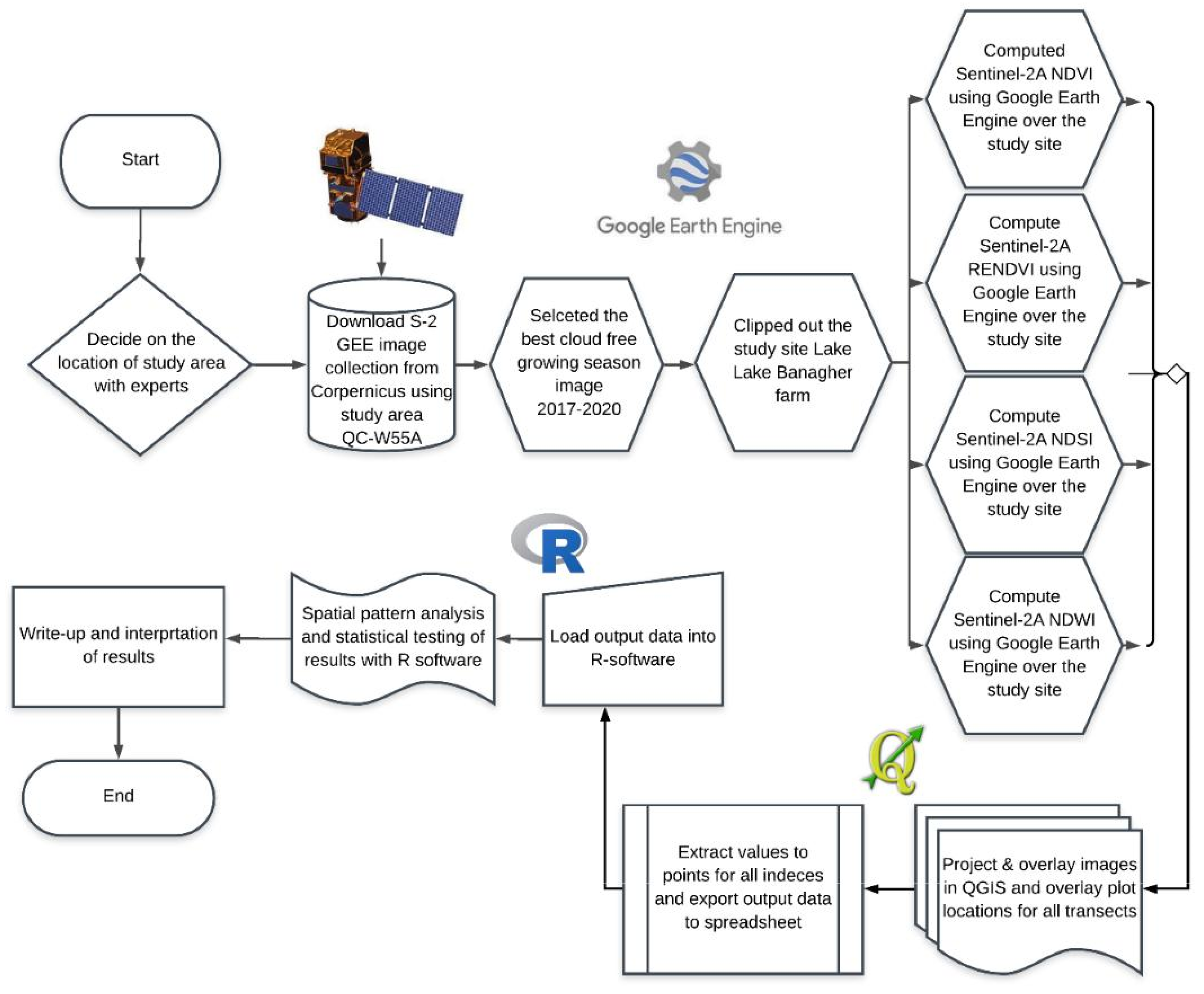
Figure 2.
Showing the positioning of the sampled transects numbered T1 to T3 (red coloured 10mX10m belt transect of plots 100m2) lines for illustration purposes. The image has been clipped to the shape of the current boundary of the Lake Banagher farm. The map was created using Sentinel-2A at the spatial resolution of 10m, a natural colour composite.
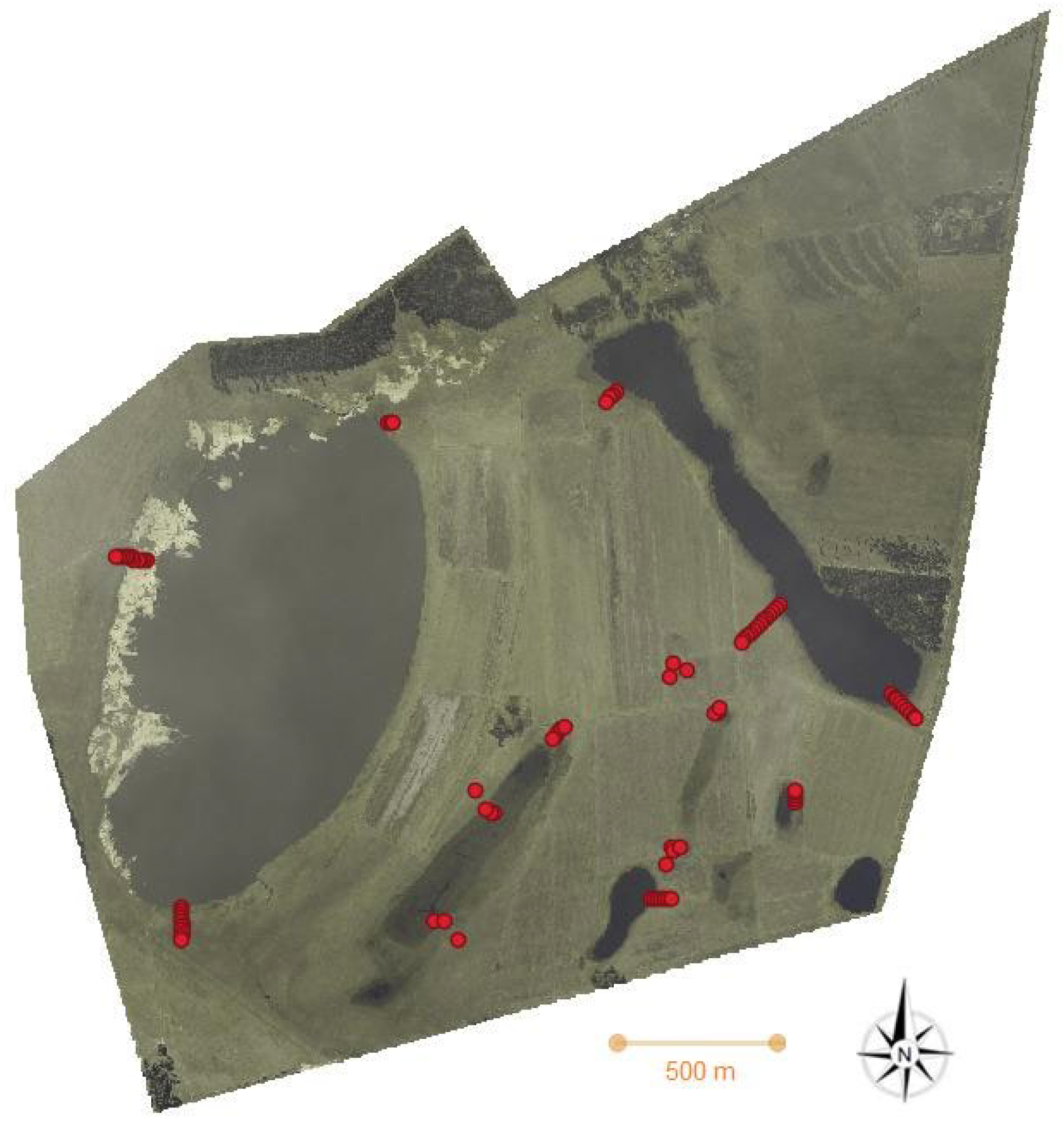
Figure 3.
Maps of indices from which the data were extracted. The classification maps were analysed using Google Earth Engine. The figure supports the study's key aim, i.e., determining littoral transition, because classifying images is critical before extracting data. Colour composites can also provide information on vegetation distribution.
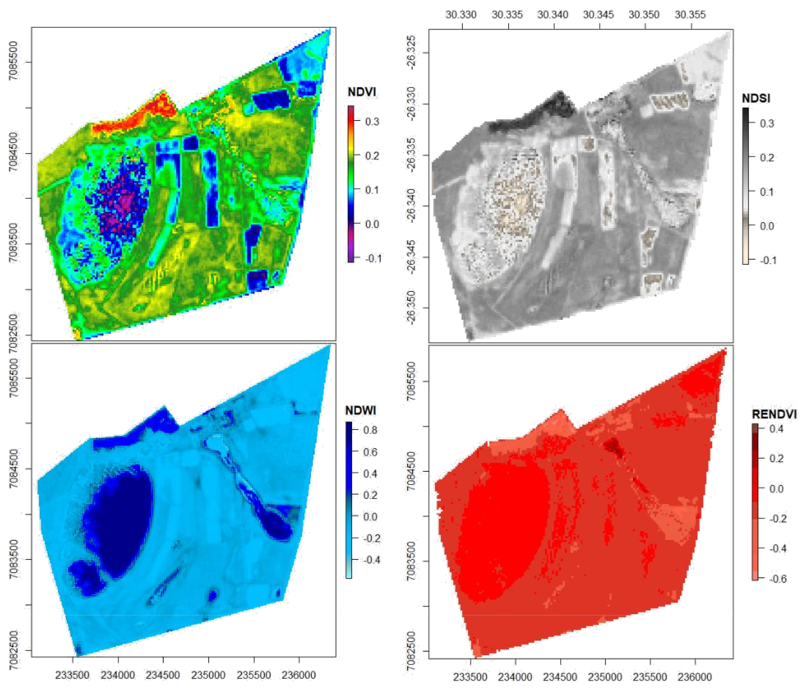
Figure 4.
Median NDWI, NDSI, RENDVI and NDVI across the eight sampled wetland sites (data that is combined by site). Data have been arranged in descending alphabetic order by site name. Sample density distributions of the eight wetlands' four vegetation remote sensing indices appear below respective horizontal boxplots, following the same colour scheme of the horizontal boxplots—projection of the variables on a 1÷4 factor-plane (right). Each data point in each of the four regions of the ordination space is influenced more by the variable correlated with the specific region.
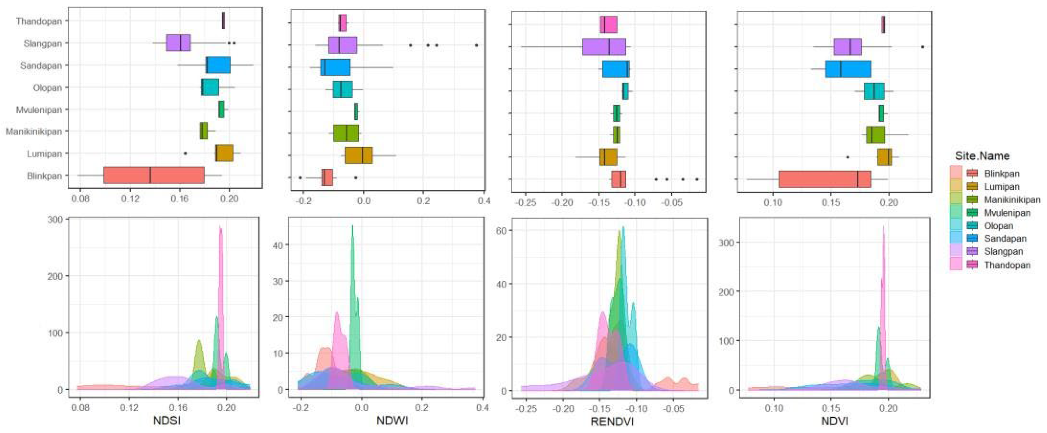
Figure 5.
PCA ordination diagram of the Lake Banagher Wetland remote sensing vegetation indices dataset with data points representing plots grouped by the site (colours).
Figure 5.
PCA ordination diagram of the Lake Banagher Wetland remote sensing vegetation indices dataset with data points representing plots grouped by the site (colours).
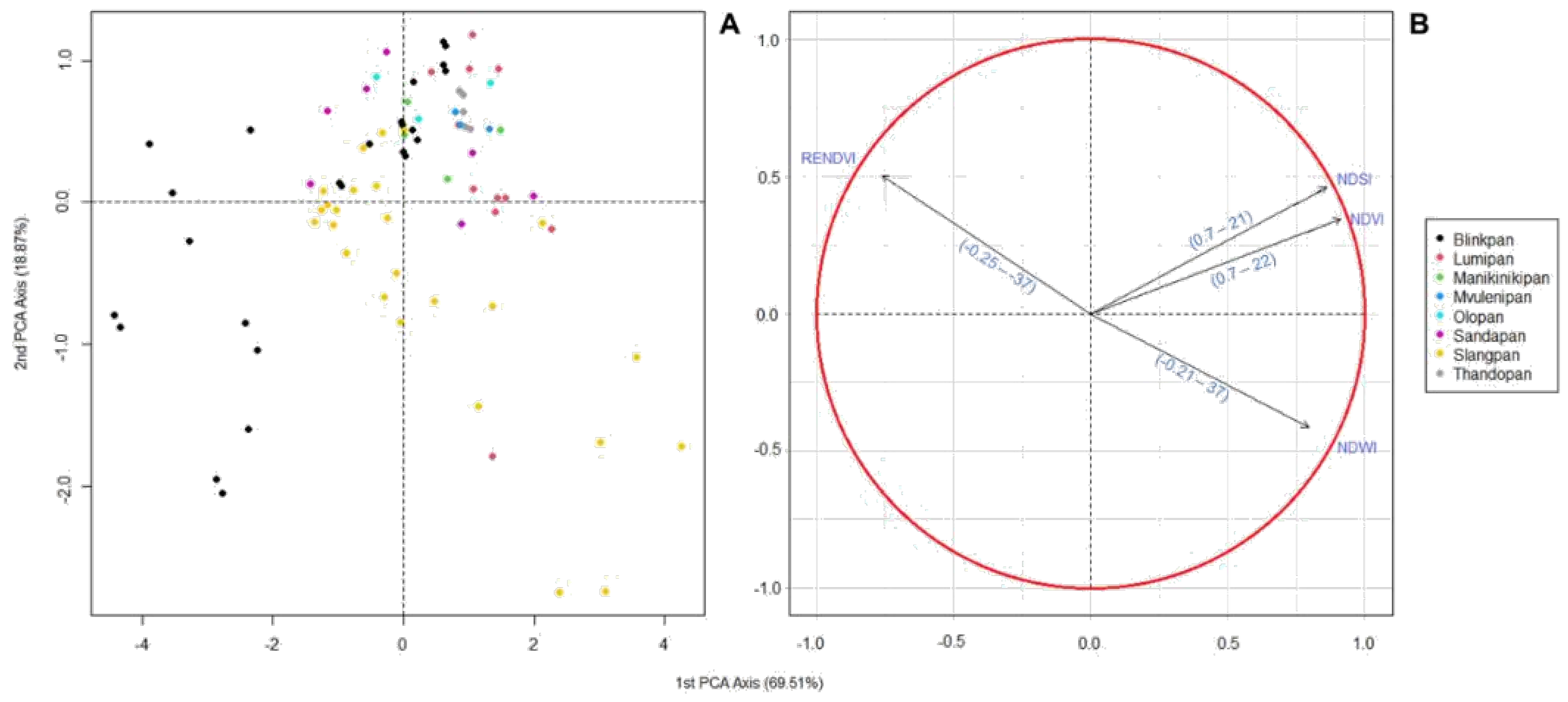
Figure 6.
Polynomial regression models of remote sensing vegetation indices to increasing distance from the edge of the wetland waterbody (solid red lines, mathematical model iterations; statistics for the model are in appendices).
Figure 6.
Polynomial regression models of remote sensing vegetation indices to increasing distance from the edge of the wetland waterbody (solid red lines, mathematical model iterations; statistics for the model are in appendices).
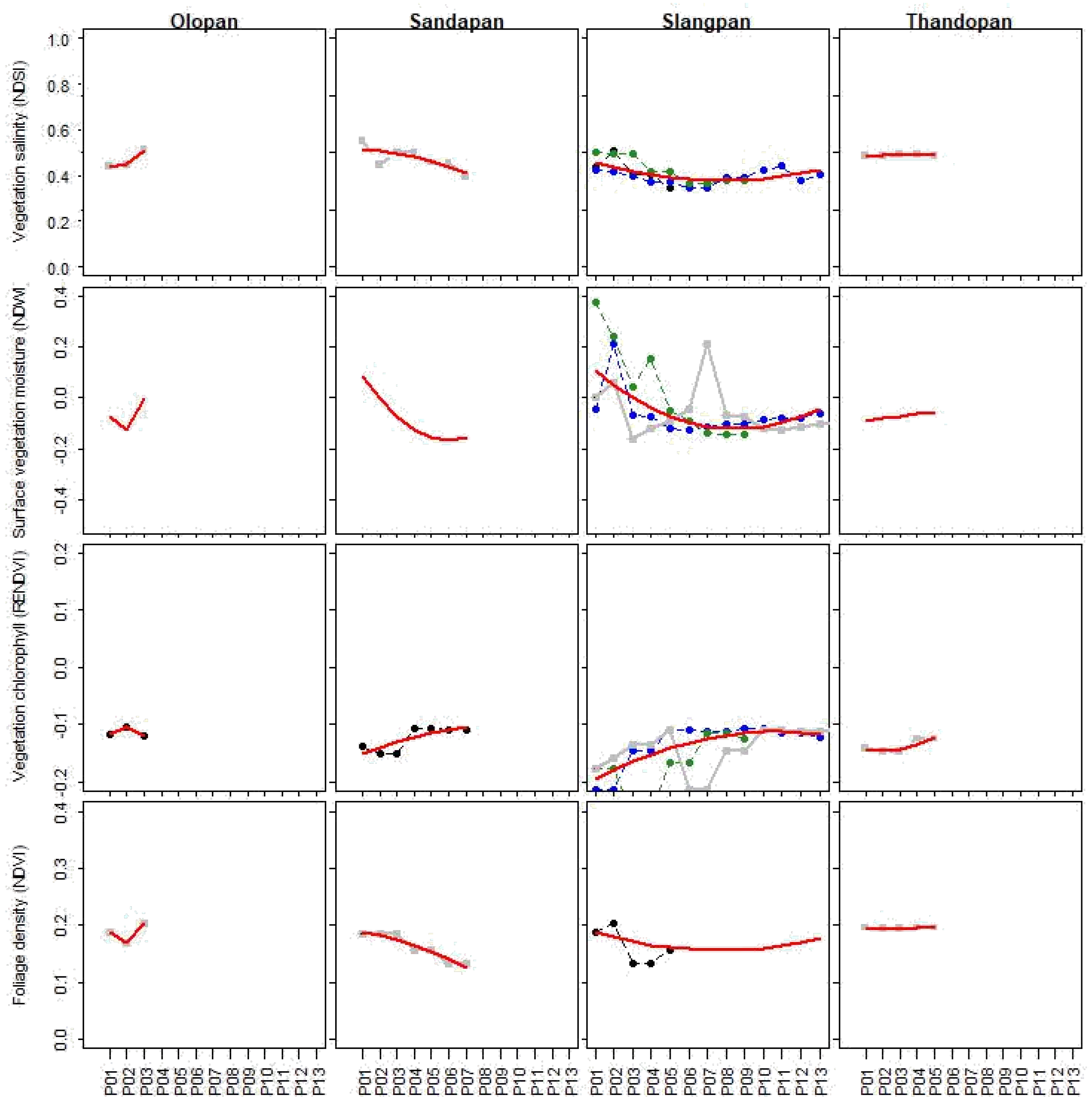
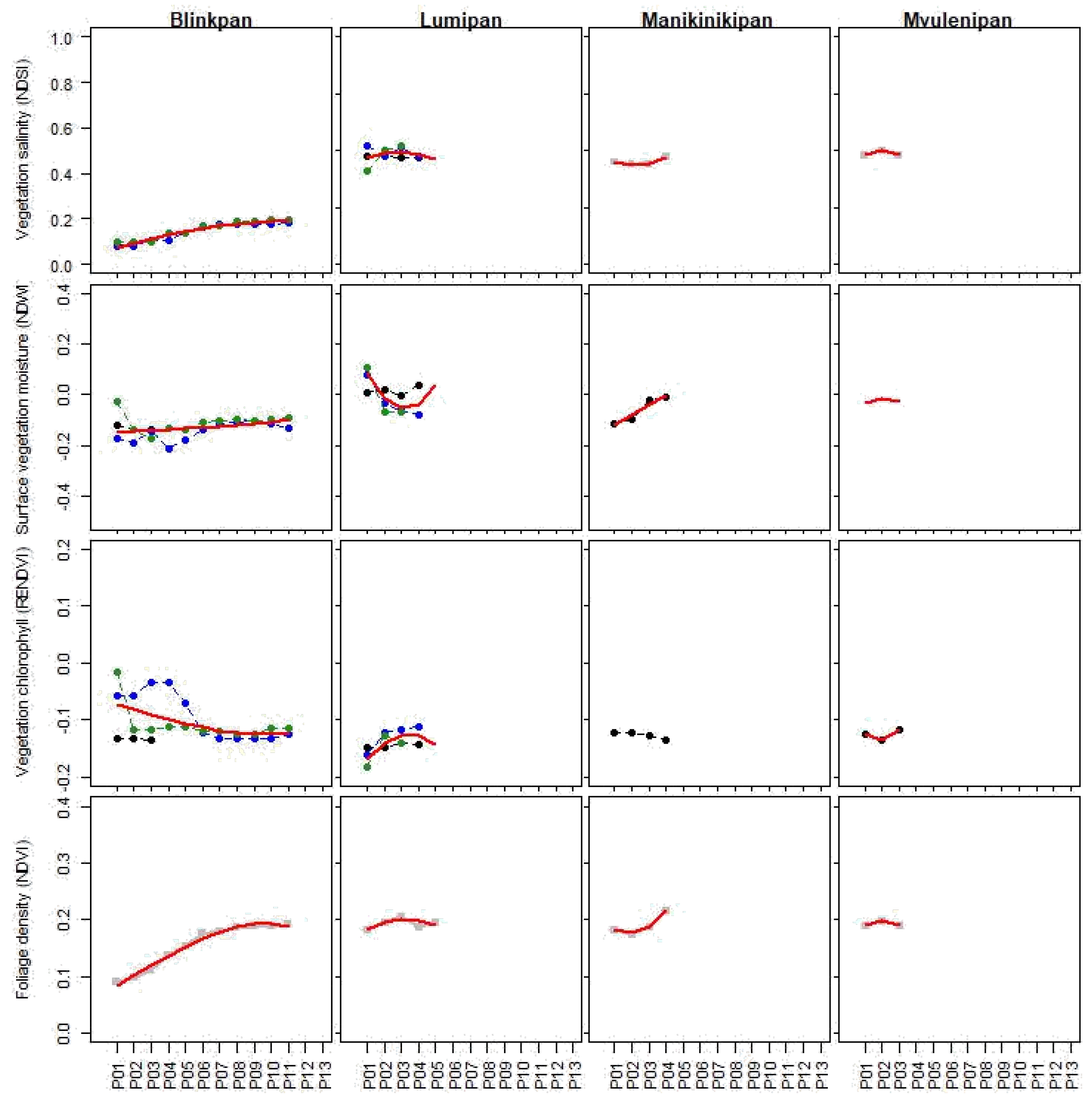
Figure 7.
Mean values of vegetation spectral indices aggregated by plot number across the littoral gradient of depression wetlands, showing adjacent groups of plots being similar in spectral indices and differences in spectral indices between the two sides of the wetland threshold.
Figure 7.
Mean values of vegetation spectral indices aggregated by plot number across the littoral gradient of depression wetlands, showing adjacent groups of plots being similar in spectral indices and differences in spectral indices between the two sides of the wetland threshold.
Disclaimer/Publisher’s Note: The statements, opinions and data contained in all publications are solely those of the individual author(s) and contributor(s) and not of MDPI and/or the editor(s). MDPI and/or the editor(s) disclaim responsibility for any injury to people or property resulting from any ideas, methods, instructions or products referred to in the content. |
© 2024 by the authors. Licensee MDPI, Basel, Switzerland. This article is an open access article distributed under the terms and conditions of the Creative Commons Attribution (CC BY) license (http://creativecommons.org/licenses/by/4.0/).
Copyright: This open access article is published under a Creative Commons CC BY 4.0 license, which permit the free download, distribution, and reuse, provided that the author and preprint are cited in any reuse.


