
Submitted:
24 June 2024
Posted:
04 July 2024
You are already at the latest version
Abstract
This paper presents a comprehensive comparative analysis of four different computational vision algorithms for implementing an unpalleting system in a factory environment, under typical edge computing constraints. The primary objective is to automate the process of detecting and locating specific variable-shaped objects on a pallet, enabling a robotic system to accurately unstack them. The four algorithms evaluated are Pattern Matching, Scale-Invariant Feature Transform, Oriented FAST and Rotated BRIEF, and Haar cascade classifiers. Each technique is described in detail in this paper, and their implementations are outlined. Experimental results are thoroughly analyzed, assessing the algorithms’ performance based on accuracy, robustness to variability, computational speed, detection sensitivity, and resource consumption. The findings reveal the strengths and limitations of each algorithm, providing valuable insights for selecting the most appropriate technique based on the specific requirements of the unpalleting system. This research contributes to the advancement of automated object detection and localization in industrial environments, paving the way for more efficient and reliable unpalleting systems.
Keywords:
Unpalleting System
; Computer Vision
; Object Detection
; Pattern Matching
; Scale-Invariant Feature Transform (SIFT)
; Oriented FAST and Rotated BRIEF (ORB)
; Haar Cascade Classifiers
; Industrial Automation
; Robotic Manipulators
; Machine Vision
1. Introduction
In modern factory settings, the process of unpalleting, which involves the ordered removal of specific objects from a pallet, is a crucial task for maintaining efficient material handling and inventory management. Traditional unpalleting methods are labour-intensive, time-consuming, and prone to errors, leading to potential safety risks and productivity losses. Consequently, there is a growing demand for automated unpalleting systems that can streamline this process, reduce human intervention, and enhance overall operational efficiency. Automated unpalleting systems equipped with robotic arms can operate continuously without fatigue, significantly increasing throughput compared to manual unpalleting. Robots can handle repetitive tasks with consistent speed and precision, leading to higher productivity and reduced cycle times. The implementation of an automated unpalleting system relies heavily on computational vision algorithms for accurate object detection and localization. These techniques leverage advanced image processing algorithms and machine learning models to identify and locate the desired objects on the pallet, enabling a robotic system to precisely pick and move them. However, the selection of the most suitable computational vision technique is a critical decision, as it directly impacts the system’s performance, reliability, and overall effectiveness, especially when performed on the edge.
This paper presents an edge computing approach to the problem with a comprehensive comparative analysis of four prominent computational vision algorithms for implementing an unpalleting system: Pattern Matching, Scale-Invariant Feature Transform (SIFT), Oriented FAST and Rotated BRIEF (ORB), and Haar Cascade classifiers [1,2,3,4,5,6,7]. Each of these algorithms offers unique strengths and limitations, and their performance is evaluated based on several key factors, including accuracy, robustness to variability, computational speed, detection sensitivity, and resource consumption.
The experimental setup is based on a Raspberry Pi 4, a camera, and a simulated physical environment. Matchboxes are used as representative objects to simulate product boxes on a pallet, and pictures are captured for experimental purposes. The implementation of each technique is described in detail, and the respective results are thoroughly analyzed and discussed. By conducting this comprehensive analysis, we aim to provide valuable insights and guidelines for selecting the most appropriate computational vision technique for the unpalleting system implementation. The findings contribute to the advancement of automated object detection and localization in industrial environments, paving the way for more efficient and reliable unpalleting processes, and ultimately enhancing productivity and operational excellence.
The paper organization is the following: in Background and Motivation we provide a foundation for understanding the current state of the art. The Methodology section details the experimental setup and the specific computational vision algorithms employed, including SIFT, ORB, and others, along with the criteria for their selection. The Results and Discussion section presents the findings from the experiments, comparing the performance of different algorithms based on metrics such as accuracy, processing time, and resource consumption. This is followed by a discussion that interprets the results, highlighting the strengths and limitations of each algorithm and their implications for practical deployment in industrial settings. The paper ends in the Conclusions summarizing the key insights and suggesting directions for future research.
2. Background and Motivation
2.1. Unpalleting Systems in Industrial Environments
Unpalleting systems play a crucial role in modern industrial environments, where efficient material handling and inventory management are vital for streamlining operations and minimizing downtime [8,9]. These systems are designed to automate the process of removing specific objects from a pallet, reducing the need for manual labour and mitigating potential safety risks associated with repetitive tasks.
Traditional unpalleting methods rely heavily on human intervention, which can be labour-intensive, time-consuming, and prone to errors. Additionally, manual unpalleting processes may expose workers to potential hazards, such as repetitive strain injuries and accidents caused by improper handling or lifting of heavy objects. To address these challenges, researchers and industry professionals have explored various approaches to automate the unpalleting process. One of the key enablers for successful automation is the integration of computational vision techniques, which leverage advanced image processing algorithms and machine learning models to accurately detect and locate the desired objects on the pallet.
2.2. Computational Vision Techniques for Object Detection and Localization
Computational vision techniques have revolutionized the field of object detection and localization, with numerous algorithms and approaches being developed and applied across various domains [10,11]. These techniques leverage sophisticated image processing algorithms and machine learning models to identify and locate specific objects within complex visual scenes [12]. Pattern Matching is a classic algorithm in image processing that involves comparing a predefined template against different regions of the target image. This technique is particularly effective when the appearance of the object is well-defined and can be represented by a template. However, its performance may be influenced by factors such as variations in scale, rotation, and illumination.
The Scale-Invariant Feature Transform (SIFT) is a robust algorithm that operates by identifying distinctive local features, or key points, within an image that is invariant to changes in scale, rotation, and illumination [3]. SIFT generates descriptors that encapsulate the local image information around each key point, enabling efficient matching between key points in different images. The Oriented FAST and Rotated BRIEF (ORB) algorithm is an efficient method for feature detection in image processing [5]. ORB starts by identifying key points using the FAST algorithm, assigns an orientation to each key point for rotation invariance, and extracts binary descriptors using BRIEF to represent local intensity patterns. This algorithm enables efficient matching between key points in different images.
Finally, Haar cascade classifiers are a machine learning-based object detection method widely used in image processing [13]. These classifiers are trained on positive and negative samples of a target object, creating a model that can efficiently identify instances of that object in new images. Haar Cascade models excel in detecting objects with specific structural patterns, making them particularly suitable for tasks like face detection. Each of these computational vision algorithms offers unique strengths and limitations, and their suitability for unpalleting system implementation depends on the already mentioned metrics, specifically tuned to take into account the time constant of edge computing tasks.
2.3. Related Work
Numerous studies have been conducted in the field of computational vision for object detection and localization, exploring various techniques and their applications in different domains. However, research specifically focused on comparative analyses of these algorithms for unpalleting system implementation is relatively limited. Regarding the application of examining applications related to vision-based depalletizing reveals an abundance of scientific literature, however, the number of methods covered by each study may be restricted and sometimes is out of date. For instance, pioneering work was done in object detection with SIFT-based clustering [1] to pick-and-place objects: while it is presented as a single technique, it is highly flexible for different objects. In another work, Ahaitouf and Mansouri [2] propose two feature selection algorithms Haar-like feature selection and Local Binary Patterns (LPB) for the detection of a single object and multiple objects in the same scene and for both standard platform and embedded system. Bansal and Kumar [14] presented the performance of various object recognition approaches in a comparative analysis of SIFT, SURF and ORB feature descriptors and multiple combinations of these feature descriptors. This experimental work was conducted using a public dataset, namely, Caltech-101.
In other research [4], the development and comparison of two distinct approaches, a machine learning strategy based on Support Vector Machine (SVM) [15] and a deep learning approach employing the YOLO (You Only Look Once) [16] network, for small target detection is analysed. Due to the restrictions in the region of interest (ROI) selection, the SVM-based method performs better in terms of computing resources and time consumption but suffers from accuracy and robustness problems in some cases, such as occlusion, illumination fluctuations, and tilting. Conversely, the YOLO network-based deep learning approach has better accuracy but has trouble in reaching real-time performance, particularly on onboard computers that have weight and power limitations.
Recent changes in the YOLO network architecture made it possible to run the system on edge devices, although the issue of latency may not be suitable for real-time operation. Furthermore, the training of deep learning algorithms requires a large amount of data, and the process of creating a dataset and manually labelling it takes a long time. As a result, various target detection techniques should be used based on the circumstances, and adjustments must be made as needed.
For these reasons, deep learning approaches are not considered in this work.
3. Methodology
3.1. Experimental Setup
The experimental setup for this research involved the utilization of an edge solution with a camera and a controlled environment. Matchboxes were used as representative objects to simulate product boxes on a pallet, and photographs were captured for experimentation purposes. The Raspberry PI4 acted as the primary computing platform, responsible for running the computational vision algorithms and processing the captured images. The camera was mounted in a fixed position, vertically placed above the pallet and roughly centered, ensuring consistent image capture and analysis. The Raspberry PI4 serves also as the central controller of our setup, orchestrating the various components. Images are captured at a resolution of 1280x720, RGB 24bpp, using the PI camera model HBV-1708 with autoFocus and a 2592x1944 maximum resolution.
Pallet items are detected on the edge device and non-maximum suppression [17] is applied to remove multiple overlapping observations. Then the position of their center is estimated and transmitted to the robot to remove the identified item from the stack and place it onto the target position (which can be a conveyor belt or another pallet, depending on the task). Ideally, at each new iteration, the algorithm must guarantee that the topmost layer is emptied before moving to the next one – although this part is out of scope for the present work.
The setup of the required equipment is illustrated in (Figure 1). The experiment showcases several feature extraction methods.
The study delves into the performance metrics of each algorithm (Pattern Matching, Haar Cascade, SIFT, and ORB) including accuracy, speed, robustness to variability, computational efficiency, detection sensitivity, and resource consumption. The proposed system is realized through the following stages (Figure 2):
- Collecting the image data.
- Preprocessing and generating feature vectors using four feature descriptors Pattern Matching, Haar Cascade, SIFT and ORB individually.
- Make a comparison between outcome algorithms.
- Finding the best algorithm.
3.2. Pattern Matching
A key role for precisely detecting and locating predetermined templates inside an image is pattern matching, which is used in image processing. With a special emphasis on the integration of template matching with non-maximum suppression, a widely used technique in this field, this section seeks to clarify the technical subtleties and approaches that underpin pattern matching.
Pattern Matching is a classical approach in image processing that involves comparing a predefined template against different regions of the target image. In this research, the implementation of Pattern Matching followed these key steps:
- Template Generation: Templates are generated by reading template images and creating various rotations to enhance detection robustness end to encapsulate the visual characteristics of objects within an image. This involves capturing template images and applying transformations such as rotations to create variations that enhance the system’s capacity to detect objects across diverse orientations.
- Image Processing: The system captured an image from the camera and converted it to grayscale, which not only simplifies subsequent computations but also facilitates robust feature extraction, essential for accurate pattern matching and proceeded with template matching.
- Template Matching: Central to the pattern matching process is template matching, realized through mathematical operations such as cross-correlation or normalized cross-correlation.
Normalized Cross-Correlation (NCC)
The NCC (or Pearson correlation coefficient) [18] is a coefficient, typically seen in its 2D version, useful for the quantification of image similarity and routinely encountered in template matching algorithms, such as in facial recognition, motion-tracking. The formula for normalized cross-correlation is:
where:
- is the correlation value at the point .
- is the pixel value in the template at position .
- is the mean of the pixel values in the template.
- is the pixel value in the image at position .
- is the mean of the pixel values in the region of the image being compared with the template.
Procedure for Template Matching
- Calculate the mean of the template:where m and n are the dimensions of the template.
- Calculate the mean of the image region:where p and q are the dimensions of the region.
- Calculate the numerator of the NCC:
- Calculate the denominator of the NCC:
- Calculate the correlation value for each position in the image.
The matchTemplate function from OpenCV [11] was employed to detect instances of the templates in the image, and a threshold was applied to filter out false positives.
- 4.
-
Non-maximum Suppression (NMS): the algorithm removes redundant bounding boxes using non-maximum suppression, ensuring only the most relevant boxes are considered. Modern object detectors usually follow a three-step recipe:
- proposing a search space of windows (exhaustive by sliding window or sparser using proposals)
- scoring/refining the window with a classifier/regressor,
- merging the bounding boxes around each detected object into a single best representative box.
This last stage is commonly referred to as “non-maximum suppression” and is a crucial step in pattern-matching algorithms to refine the detected object locations and eliminate redundant matches. NMS can be used to find distinctive feature points in an image. To improve the repeatability of a detected corner across multiple images, the corner is often selected as a local maximum whose cornerness is significantly higher than the close-by second-highest peak [19]. NMS with a small neighborhood size can produce an oversupply of initial peaks. These peaks are then compared with other peaks in a larger neighborhood to retain strong ones only. The initial peaks can be sorted during NMS to facilitate the later pruning step.For some applications such as multi-view image matching, an evenly distributed set of interest points for matching is desirable. An oversupplied set of NMS point features can be given to an adaptive non-maximal suppression process [6], which reduces cluttered corners to improve their spatial distribution.Consider a similarity score matrix obtained after template matching, where u and v represent the coordinates of the image. Each element denotes the similarity score at the corresponding location in the image. The non-maximum suppression algorithm can be described as followsIn this formulation:- represents the resulting score after non-maximum suppression.
- For each pixel location the algorithm checks whether the similarity score at that location is greater than or equal to the scores of its neighboring pixels in all eight directions (i.e., top-left, top, top-right, left, right, bottom-left, bottom, bottom-right).
- If the similarity score at is greater than or equal to the scores of all its neighbors, it is retained as a local maximum and assigned the same value.
- Otherwise, if is not a local maximum, it is suppressed by setting its value to zero.
This process ensures that only the highest-scoring pixel in each local neighbourhood is retained, effectively removing redundant detections, and preserving only the most salient object instances in the image. By employing non-maximum suppression, pattern-matching algorithms can produce more accurate and concise results, facilitating precise object localization and recognition within complex visual scenes.
- 5.
- Result Visualization: The final result was displayed, indicating the detected objects’ centres and their corresponding identification numbers (Figure 3).
Scale-Invariant Feature Transform (SIFT)
The Scale-Invariant Feature Transform (SIFT) is a robust algorithm for keypoint detection and feature matching in image processing [3]. This algorithm extracts the features of an object considering different scales, rotations, illumination, and geometric transformations. SIFT has been proven the most widely used algorithm in object recognition. It obtains the image as an input and produces a set of features as output. SIFT works in four phases:
- Scale-space Extrema Detection
- Keypoint Localization
- Orientation Assignment
- Keypoint Descriptor
SIFT builds a multi-resolution pyramid over the input image and has proved to be very robust to noise and invariant to scaling, rotation, translation and (to some extent) illumination changes. First, the Difference of Gaussian (DoG) is applied to detect local extrema (keypoint) in space scale. Second, more accurate locations of key points are determined using threshold values. The third stage assigned the orientation to describe the key points with invariance to image rotation.
In this method, the SIFT detector is initialized, and a Brute Force Matcher is created for keypoint matching. Key points and descriptors are computed for template images and the target image, respectively. Matches between descriptors are filtered, and a minimum match count is set to ensure accurate object detection. The perspective transformation matrix is computed using the matched key points, and the bounding box of the object is determined. The bounding box and centre of each detected object are visualized on the target image. In the provided code, there are a few preprocessing steps applied to the images before performing object detection.
The implementation of SIFT in this research followed these steps:
- SIFT Feature Extraction: SIFT key points and descriptors are extracted from both the template and target images. This step involves analyzing the local intensity gradients of the images to identify distinctive key points and generate corresponding descriptors.
- Looping Over Image Regions: The code iterates over different regions of the target image using nested loops. Within each iteration, a region of interest (ROI) is defined based on the current position of the loop.
- Matching and Filtering: Matches between descriptors were filtered, and a minimum match count was set to ensure accurate object detection.
- Filtering Matches: A ratio test is applied to filter out good matches from the initial set of matches. Only matches with a distance ratio less than a certain threshold are considered as good matches. The threshold refers to a distance ratio used in the ratio test for filtering good matches. The ratio test compares the distances between the nearest descriptor and the second one in each descriptor.
- Homography Estimation: Using the RANSAC algorithm (Random Sample Consensus), a perspective transformation matrix (M) is estimated based on the good matches. This matrix represents the geometric transformation required to align the template image with the current ROI (Region of Interest) in the target image.
- Perspective Transformation: The computed transformation matrix is used to alter the corners of the template picture such that they line up with the ROI in the target image.
- Bounding Box Computation: The minimum and maximum coordinates of the transformed corners are calculated to determine the bounding box of the detected object in the target image.
-
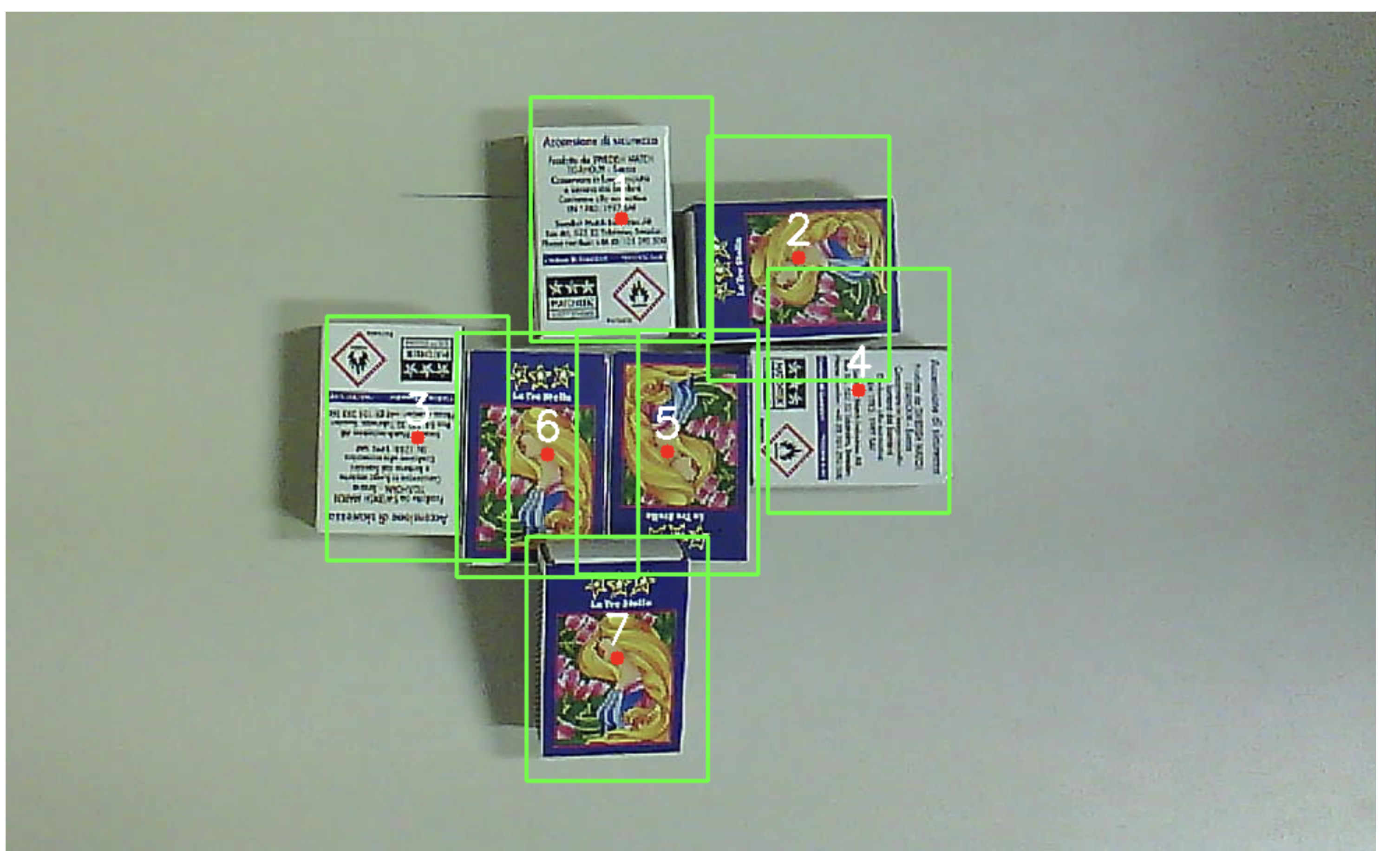
Drawing and Visualization: Finally, the bounding box and centre of the detected object are selected on the target image.Overall, the main preprocessing step used in the SIFT technique is feature extraction, and there are SIFT key points and descriptors calculated in both the template and target images. Then these descriptors are used for matching and finally object detection. In this technique, the code does not include explicit preprocessing steps such as image resizing, noise reduction, or contrast enhancement.The result of detection is shown in Figure 4.
Oriented FAST and Rotated BRIEF (ORB)
The Oriented FAST and Rotated BRIEF (ORB) algorithm is an efficient method for feature detection and matching in image processing, presented for the first time by Rublee and his colleagues [5]. Compared to SIFT and SURF, ORB is substantially faster in the usual situation.
The Oriented FAST and Rotated BRIEF (ORB) algorithm is a robust and efficient method for feature detection in image processing. ORB starts by identifying key points using the FAST algorithm, which efficiently locates areas with significant intensity changes. Unlike traditional FAST, ORB assigns an orientation to each key point, ensuring rotation invariance. The algorithm then extracts binary descriptors using BRIEF, representing the local intensity patterns around each key point. These descriptors enable efficient matching between key points in different images.
The matching process involves comparing the binary descriptors of key points in the target image with those in a reference template. A Brute Force Matcher is commonly used for this task. After matching, a filtering step eliminates unreliable matches, and the algorithm considers regions with a sufficient number of good matches as potential detections. Non-maximum suppression is applied to merge nearby detections, ensuring a concise and accurate set of identified objects. The final result is a representation of detected objects with bounding boxes, providing a foundation for further applications in object recognition and computer vision tasks. The ORB implementation in this research involved the following steps:
- Implements the ORB detector for feature extraction in both the template and target image.
- Applies a sliding window approach with a defined step size for efficient detection.
- Utilizes a Brute-Force Matcher with Hamming distance for descriptor matching.
- Filters match based on a predefined matching threshold.
- Performs non-maximum suppression to merge nearby bounding boxes.
Marks the centre of each bounding box and assigns a unique identifier for robot coordination. The result of detection is shown in Figure 5.
As it can be observed, while reliable for the front side of objects, it shows limitations in recognizing the back part of boxes. However, it maintains acceptable detection accuracy under certain conditions. It displays limitations in recognizing specific object orientations, impacting its robustness to variability. However, it remains reliable under certain conditions as well. ORB Exhibits the slowest execution speed in implementation, contrary to expectations for a binary method, suggesting potential performance optimizations, requiring careful parameter tuning for optimal performance. This technique is able to work with restricted resources.
3.5. Haar Cascade Classifiers
Haar Cascades is a machine learning-based object detection method widely used in image processing. A Haar Cascade classifier operates by training on positive and negative samples of a target object, creating a model that can efficiently identify instances of that object in new images. During training, the classifier learns to recognize distinctive features that characterize the object of interest. These features are essentially rectangular filters applied to different regions of the image, and the classifier assesses whether the intensity patterns in these rectangles match the learned patterns from positive samples.
Once trained, a Haar Cascade classifier is applied to an image through a sliding window approach. The classifier evaluates each window by efficiently applying a series of feature comparisons at different scales and positions. If a region of the image matches the learned pattern for the object, the classifier identifies it as a positive detection. Haar Cascades are computationally efficient. However, they may have limitations in handling complex backgrounds or objects with varying orientations, as the training data needs to encompass diverse instances of the target object for optimal performance.
The given Python code trains a Haar Cascade classifier with OpenCV for object identification, creates a positive picture and various negative datasets, and generates positive examples [13]. The primary steps are listed as follows:
- Prepare Negative Images: A folder for negative images was created by copying images from a source directory. A background file (bg.txt) listed the negative images.
- Resize and Edit Images: Positive and negative images were resized to consistent dimensions (e.g., 60x100 pixels for positive images). For positive images, an option is provided to either use default dimensions or customize the size. The script renames the images and adjusts their dimensions accordingly.
- Create Positive Samples: The tool generated positive samples and related information for each positive image. The program iterates through the positive images, creating a separate directory for each image’s data. The default configuration includes parameters like angles, number of samples, width, and height.
- Merge Vector Files: Positive sample vector files were merged into a single file (mrgvec.vec) for training input.
- Train Cascade Classifier: The tool trained the Haar Cascade classifier using configuration options like the number of positive/negative samples and stages. The training process can be run in the background if specified.
- Completion: Despite a time-intensive training process, Haar Cascade exhibits effective detection performance, resulting in acceptable in proper accuracy. Moreover, it shows resilience to variations in expressions and lighting conditions, contributing to its effectiveness in real-world scenarios. Concerning its computational speed, it demonstrates quick detection post-training, with the inevitable and initial time investment required during the training phase. It requires attention to parameters such as setting variation, rotation angle and different thresholds contributing to the time-consuming tuning process. In this approach significant computational resources during the training phase, with efficient resource consumption during detection in a large number of negative images and a few positive images (Figure 6).
4. Results and Discussion
The performance of each computational vision technique was evaluated based on several key factors: accuracy, robustness to variability, computational speed, detection sensitivity, and resource consumption. The results are presented and discussed in the following sections.
4.1. Accuracy
- Pattern Matching: Achieved high accuracy in object detection, with straightforward configuration by adjusting a single threshold and angle.
- SIFT: Demonstrated efficiency in finding key points, especially effective in rotation scenarios, contributing to its versatility across various applications.
- ORB: Maintained reliable detection accuracy for the front side of objects under certain conditions but showed limitations in recognizing the back part of matchboxes.
- Haar Cascade: Despite a time-intensive training process, Haar Cascade exhibited effective detection performance, resulting in acceptable accuracy.
4.2. Robustness to Variability
- Pattern Matching: Demonstrated robustness to variability, showcasing resilience to changes in object appearance, lighting, and orientation.
- SIFT: Proved robust against scale, rotation, and illumination changes, contributing to its adaptability in diverse conditions.
- ORB: Displayed limitations in recognizing specific object orientations, impacting its robustness to variability. However, it remained reliable under certain conditions.
- Haar Cascade: Showed resilience to variations in object appearance and lighting conditions, contributing to its effectiveness in real-world scenarios.
4.3. Computational Speed
- Pattern Matching: Achieved fast detection speed, taking only a few seconds for implementation.
- SIFT: Boasted a fast implementation with efficient key point detection, contributing to its real-time applicability.
- ORB: Exhibited slower execution speed, contrary to expectations for a binary method, suggesting potential performance optimizations.
- Haar Cascade: Demonstrated quick detection post-training, with the inevitable and initial time investment required during the training phase.
4.4. Detection Sensitivity
- Pattern Matching: Exhibited sensitivity to changes in the detection threshold, offering flexibility in configuration.
- SIFT: Showed sensitivity to parameter adjustments, with a relatively quick tuning process.
- ORB: Displayed sensitivity to object orientation, requiring careful parameter tuning for optimal performance.
- Haar Cascade: Required attention to parameters such as setting variation and rotation angle, contributing to the time-consuming tuning process.
4.5. Resource Consumption
- Pattern Matching, SIFT, and ORB: Demonstrated efficient resource consumption, making them suitable for practical applications.
- Haar Cascade: Required significant computational resources during the training phase, with efficient resource consumption during detection. (requiring a large number of negative images and a few positive images)
The experimental analysis conducted in this study provides a detailed comparison of four distinct object detection algorithms: Pattern Matching, Haar Classifier, SIFT, and ORB. Each method was evaluated based on a set of performance metrics, including training time, detection time, total matches, precision, recall, and F1 score. The results provide valuable insights into the strengths and limitations of each technique, facilitating informed decisions for future applications in industrial automation and robotics.
The comparative analysis of the four algorithms—Pattern Matching, Haar Classifier, SIFT, and ORB—reveals distinct strengths and limitations across various performance metrics and computational aspects. The results are summarized in the Table 1.

Table 1.
Results of Comparing Algorithms
| Training Time (hrs) | Latency (sec) | Total Matches | Precision | Recall | F1 Score | |
|---|---|---|---|---|---|---|
| Pattern Matching | 0 | 0.13 | 7 | 1.00 | 1.00 | 1.00 |
| Haar Classifier | 3.55 | 0.0951 | 7 | 1.00 | 1.00 | 1.00 |
| SIFT | 0 | 0.388 | 6 | 1.00 | 0.857 | 0.923 |
| ORB | 0 | 12.06 | 4 | 1.00 | 0.571 | 0.727 |
Training Time
- Pattern Matching, SIFT and ORB: These algorithms do not require training, making them advantageous in scenarios where rapid deployment is needed.
- Haar Classifier: Requires a substantial training time of 3.55 hours, indicating an initial setup cost. However, this investment pays off with excellent detection performance.
Latency
- Haar Classifier: The fastest detection time (0.0951 sec) highlights its efficiency post-training.
- Pattern Matching: Quick detection time (0.13 sec) without the need for training makes it a strong candidate for real-time applications.
- SIFT: Moderate detection time (0.388 sec) reflects its computational complexity due to the detailed feature extraction process.
- ORB: Surprisingly, ORB takes the longest detection time (12.06 sec), which is unexpected for a binary feature descriptor. This may be attributed to implementation details or the specific test conditions.
Total Matches
- Pattern Matching and Haar Classifier: Both achieve the highest number of matches (7), indicating high effectiveness in object detection.
- SIFT: Slightly lower total matches (6), reflecting its robustness but also its selective nature.
- ORB: The lowest total matches (4), highlighting potential limitations in detecting all relevant objects, especially in more complex scenes.
Precision, Recall, and F1 Score
- Precision: All four algorithms exhibit perfect precision (1.00), indicating that when they do make detections, they are consistently accurate.
- Recall: Pattern Matching and Haar Classifier achieve perfect recall (1.00), showing their ability to detect all relevant objects. SIFT has a slightly lower recall (0.857), while ORB has the lowest (0.571), indicating it misses more objects.
- F1 Score: The F1 Score combines precision and recall into a single metric. Pattern Matching and Haar Classifier both achieve the highest possible F1 score (1.00). SIFT has a respectable F1 score (0.923), while ORB lags behind at 0.727.
5. Conclusions
This research presented a comprehensive comparative analysis of four prominent computational vision algorithms for implementing an unpalleting system under computational resources constraints: Pattern Matching, Scale-Invariant Feature Transform (SIFT), Oriented FAST and Rotated BRIEF (ORB), and Haar Cascade classifiers [1,2,3,4,5,6].
These algorithms are all able to work with low latency on an edge system with few computational resources such as the Raspberry Pi4. Each technique was thoroughly described, and their respective implementations were outlined. Experimental results were analyzed, assessing the algorithms’ performance based on accuracy, robustness to variability, computational speed, detection sensitivity, and resource consumption.
The findings revealed that Pattern Matching achieved high accuracy in object detection with a straightforward configuration process. SIFT proved robustness against scale, rotation, and illumination changes, contributing to its versatility across various applications. ORB displayed limitations in recognizing specific object orientations but remained reliable under certain conditions. Haar Cascade classifiers, despite a time-intensive training process, exhibited effective detection performance and acceptable accuracy.
The selection of the most suitable technique depends on the specific requirements of the unpalleting system, considering factors such as accuracy, robustness, computational speed, and resource constraints. Each method exhibited strengths and limitations, and the optimal choice may vary based on the application’s unique characteristics. Future research in this area could explore the integration of multiple computational vision techniques to leverage their respective strengths and mitigate their limitations. Additionally, investigating advanced deep learning-based object detection methods and their applicability to unpalleting systems could further enhance the system’s performance and robustness even when not running on a Raspberry.
Overall, this research contributes to the advancement of automated object detection and localization in industrial environments, paving the way for more efficient and reliable unpalleting processes, ultimately enhancing productivity and operational excellence in factory settings.
Author Contributions
Danilo Greco: conceptualization, supervision, methodology, writing, drafting of the article, review and editing, Majid Fasihiany and Ali Varasteh Ranjbar: software implementation, experiments and data curation; Francesco Masulli Stefano Rovetta and Alberto Cabri: conceptualization, visualization, supervision, review. All authors have read and agreed to the published version of the manuscript
Funding
This research received no external funding
Funding
This research received no external funding
Conflicts of Interest
The authors declares no conflict of interest.
References
- Piccinini, P.; Prati, A.; Cucchiara, R. Real-time object detection and localization with SIFT-based clustering. Image and Vision Computing 2012, 30, 573–587. [Google Scholar] [CrossRef]
- Guennouni, S.; Ahaitouf, A.; Mansouri, A. A Comparative Study of Multiple Object Detection Using Haar-Like Feature Selection and Local Binary Patterns in Several Platforms. Modelling and simulation in Engineering 2015, 2015, 948960. [Google Scholar] [CrossRef]
- Lowe, D.G. Distinctive image features from scale-invariant keypoints. International journal of computer vision 2004, 60, 91–110. [Google Scholar] [CrossRef]
- Wang, J.; Jiang, S.; Song, W.; Yang, Y. A comparative study of small object detection algorithms. In Proceedings of the 2019 Chinese control conference (CCC). IEEE; 2019; pp. 8507–8512. [Google Scholar]
- Rublee, E.; Rabaud, V.; Konolige, K.; Bradski, G. ORB: An efficient alternative to SIFT or SURF. In Proceedings of the 2011 International conference on computer vision. Ieee; 2011; pp. 2564–2571. [Google Scholar]
- Brown, M.; Szeliski, R.; Winder, S. Multi-image matching using multi-scale oriented patches. In Proceedings of the 2005 IEEE Computer Society Conference on Computer Vision and Pattern Recognition (CVPR’05). IEEE, 2005, Vol. 1, pp. 510–517.
- Muja, M.; Lowe, D.G. Fast approximate nearest neighbors with automatic algorithm configuration. VISAPP (1) 2009, 2, 2.
- Bay, H.; Tuytelaars, T.; Van Gool, L. Surf: Speeded up robust features. In Proceedings of the Computer Vision–ECCV 2006: 9th European Conference on Computer Vision, Graz, Austria, May 7-13, 2006. Proceedings, Part I 9. Springer, 2006, pp. 404–417.
- Gue, K. Automated Order Picking. In Warehousing in the global supply chain: Advanced models, tools and applications for storage systems; Manzini, R., Ed.; Springer, 2012; pp. 151–174.
- Li, Y.; Qi, H.; Dai, J.; Ji, X.; Wei, Y. Fully convolutional instance-aware semantic segmentation. In Proceedings of the Proceedings of the IEEE conference on computer vision and pattern recognition, 2017, pp. 2359–2367.
- Bradski, G.; Kaehler, A. Learning OpenCV: Computer vision with the OpenCV library; " O’Reilly Media, Inc.", 2008.
- Wuest, T.; Weimer, D.; Irgens, C.; Thoben, K.D. Machine learning in manufacturing: advantages, challenges, and applications. Production & Manufacturing Research 2016, 4, 23–45. [Google Scholar]
- Viola, P.; Jones, M. Rapid object detection using a boosted cascade of simple features. In Proceedings of the Proceedings of the 2001 IEEE computer society conference on computer vision and pattern recognition.; p. 200120011.
- Bansal, M.; Kumar, M.; Kumar, M. 2D object recognition: a comparative analysis of SIFT, SURF and ORB feature descriptors. Multimedia Tools and Applications 2021, 80, 18839–18857. [Google Scholar] [CrossRef]
- Cortes, C.; Vapnik, V. Support-vector networks. Machine learning 1995, 20, 273–297. [Google Scholar] [CrossRef]
- Redmon, J.; Divvala, S.; Girshick, R.; Farhadi, A. You only look once: Unified, real-time object detection. In Proceedings of the Proceedings of the IEEE conference on computer vision and pattern recognition, 2016, pp. 779–788.
- Bodla, N.; Singh, B.; Chellappa, R.; Davis, L.S. Soft-NMS–improving object detection with one line of code. In Proceedings of the Proceedings of the IEEE international conference on computer vision, 2017, pp. 5561–5569.
- Rodgers, J.L.; Nicewander, W.A. Thirteen Ways to Look at the Correlation Coefficient. The American Statistician 1988, 42, 59–66. [Google Scholar] [CrossRef]
- Schmid, C.; Mohr, R.; Bauckhage, C. Evaluation of interest point detectors. International Journal of computer vision 2000, 37, 151–172. [Google Scholar] [CrossRef]
Figure 1.
Reference setup.
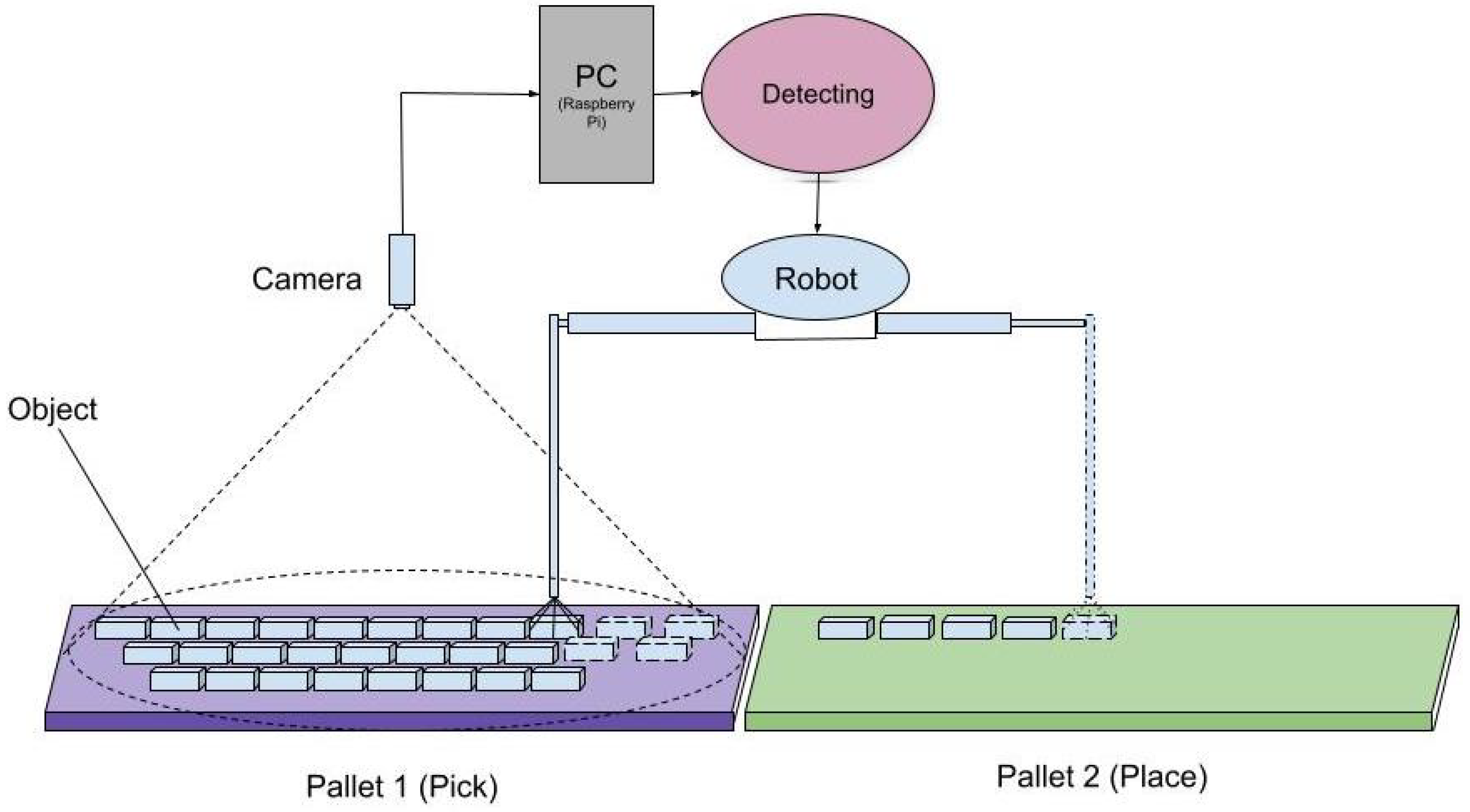
Figure 2.
Block Diagram of the experimental comparison methodology.
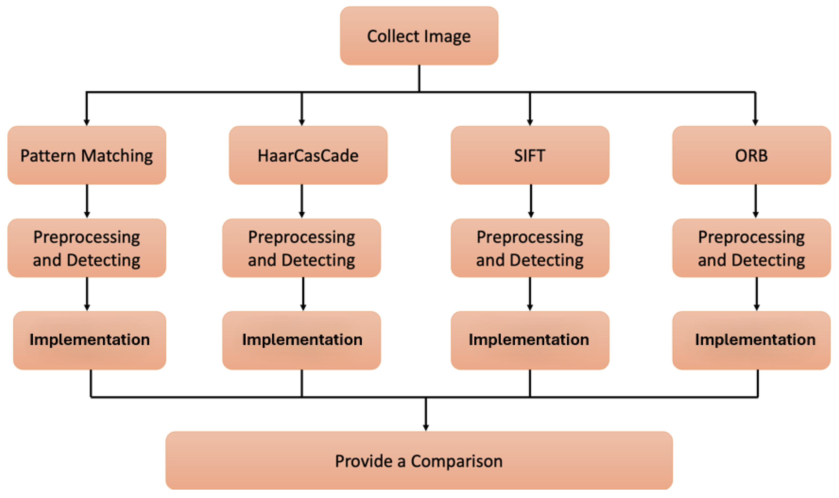
Figure 3.
Detection of Pattern Matching technique tested on matches boxes.
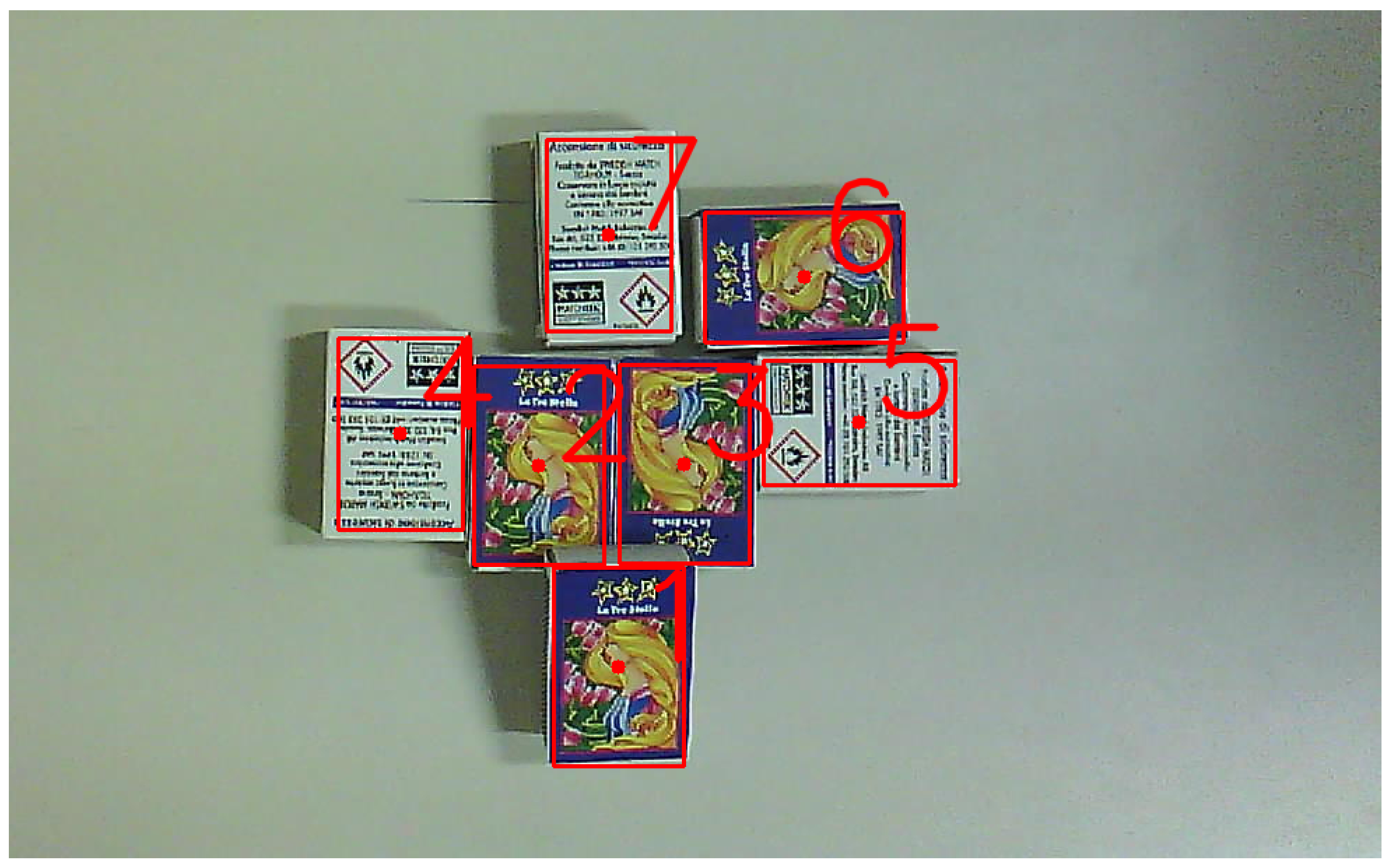
Figure 4.
Detection of SIFT technique tested on matches boxes.
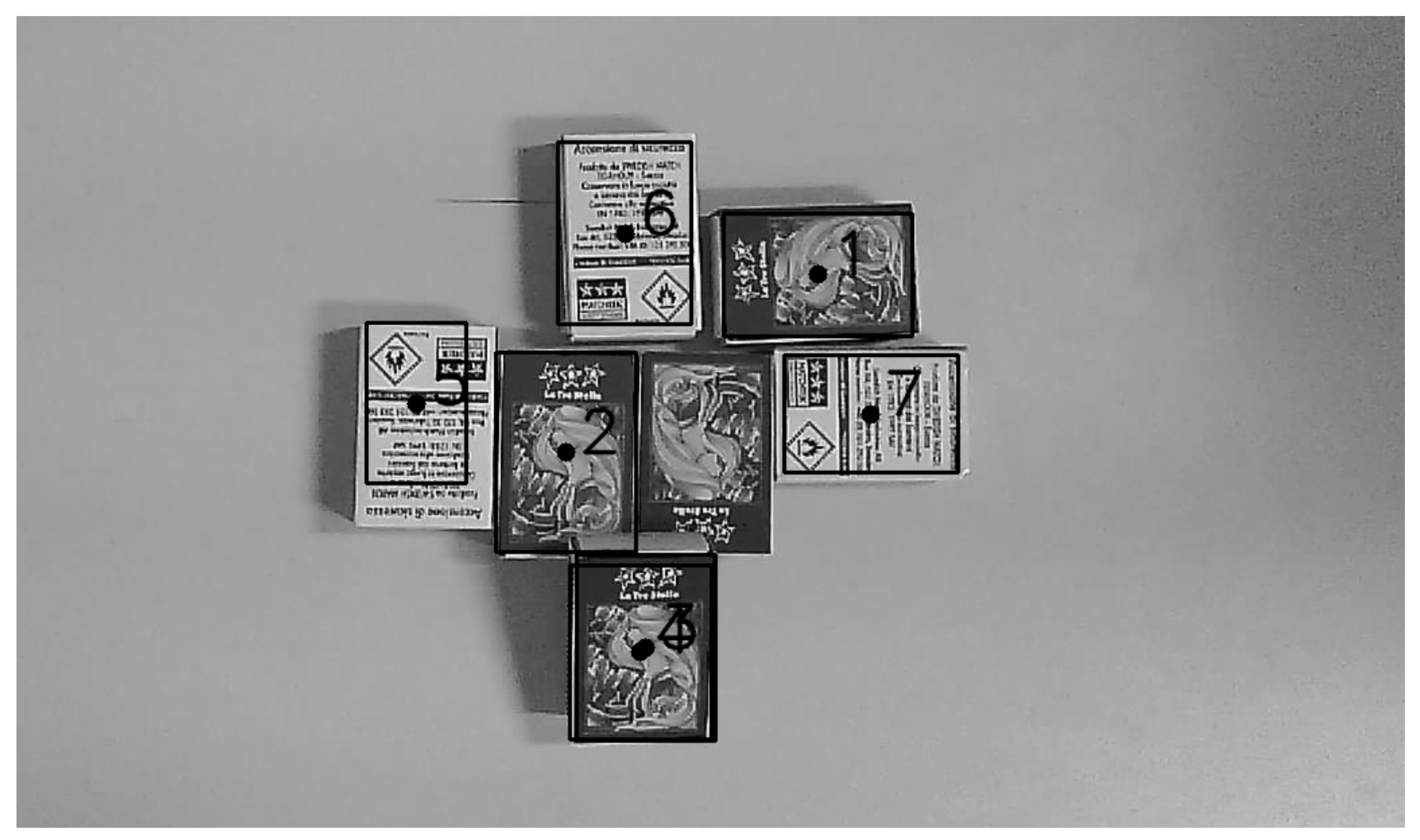
Figure 5.
Detection of ORB technique tested on matches boxes.
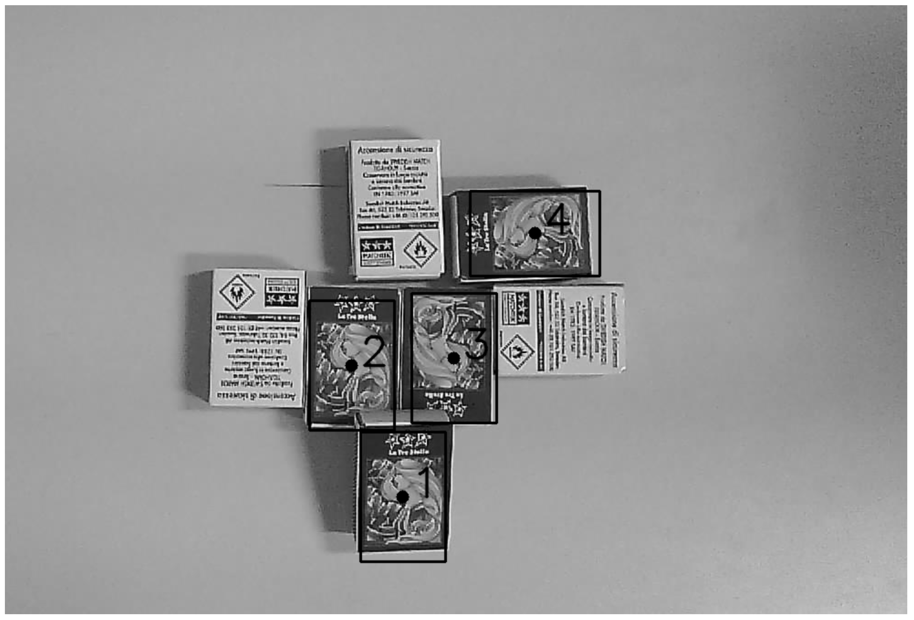
Figure 6.
Detection of Haar Classifier technique tested on matches boxes.
Disclaimer/Publisher’s Note: The statements, opinions and data contained in all publications are solely those of the individual author(s) and contributor(s) and not of MDPI and/or the editor(s). MDPI and/or the editor(s) disclaim responsibility for any injury to people or property resulting from any ideas, methods, instructions or products referred to in the content. |
© 2024 by the authors. Licensee MDPI, Basel, Switzerland. This article is an open access article distributed under the terms and conditions of the Creative Commons Attribution (CC BY) license (http://creativecommons.org/licenses/by/4.0/).
Copyright: This open access article is published under a Creative Commons CC BY 4.0 license, which permit the free download, distribution, and reuse, provided that the author and preprint are cited in any reuse.


