Submitted:
03 July 2024
Posted:
03 July 2024
You are already at the latest version
Abstract
The Katerini-Kolindros aquifer system (KKas) is a critical freshwater resource, essential for the local and regional economy. To understand contamination sources, groundwater flow paths, and assess the aquifer's health, an extensive dataset of 751 samples from 113 wells collected between 2010 and 2020 was analyzed using multivariate statistical analysis (MVSA) and hydrogeochemical diagrams. The prevailing water types identified were Ca-HCO₃ and Mg-HCO₃, with mixed water types resulting from various factors affecting groundwater quality. The chemistry of groundwater in the KKas is shown to be affected by ion exchange processes and to a lesser extent by reverse ion exchange processes. No indications of sea-water intrusion have been identified in the water wells monitored. On the other hand, nitrate contamination has been detected in specific water wells spatially associated with urban-type land uses and activities. It is considered that nitrate contamination originates primarily from septic tanks and urban sewage networks or secondarily from fertilization of football pitches, cemeteries or urban waste management practices.
Keywords:
groundwater
; hydrochemistry
; granular aquifer
; multivariate statistics
; Piper diagram
; Katerini – Kolindros
1. Introduction
Freshwater is indispensable for sustaining life and supporting ecosystems, playing a pivotal role in human well-being and environmental integrity [1]. Among its various forms, groundwater emerges as a crucial resource, underpinning ecosystem services and driving socio-economic development on a global scale [2]. However, the management of groundwater entails navigating a delicate balance between meeting human needs and conserving environmental health, with the understanding of hydrogeochemistry serving as a linchpin in this endeavor. Groundwater management represents a multifaceted challenge, intertwined with human activities, ecological demands, and geological processes. At the heart of this challenge lies the need to comprehend the hydrogeochemical dynamics governing groundwater systems. Hydrogeochemistry is essential for assessing groundwater quality and identifying the processes that affect it, making it a critical component for effective management and utilization of groundwater resources [3,4].
Groundwater quality offers invaluable insights into complex dynamics, providing a roadmap for sustainable management practices (e.g. [5,6,7,8]). Groundwater systems are often complex and require a comprehensive understanding of various geological and hydrological factors for sustainable management, with hydrogeochemistry being a critical component of this understanding [9]. Toward this goal, hydrogeochemical analysis helps identify the sources of solutes in groundwater and the processes affecting water composition (e.g. leaching, evaporation, ion exchange, human activities etc.), which are vital for assessing and managing groundwater quality [3,10,11]. Hydrogeochemical studies further contribute to assess the suitability of groundwater for various uses, such as irrigation or potability, in a sustainable manner [12,13].
A variety of techniques are used in hydrogeochemical surveys to evaluate groundwater quality. A common approach for hydrogeochemical assessments involves combining hydrochemical analysis to identify primary processes and water types, using plots such as Piper and ionic ratio plots, as well as diagrams like Gibbs and Wilcox. Additionally, spatial interpolation maps and multivariate statistical analyses (Q-mode and R-mode) are utilized. Examples of studies employing these methods include those in [14,15,16]. Additionally, other tools including tracer methods, hydrologic budget approaches, and numerical models, are available for estimating groundwater recharge, which is also critical in supporting groundwater quality evaluations [17].
The understanding of hydrogeochemical conditions and groundwater quality is essential for effective management and sustainable utilization of water resources, such as for drinking and agricultural purposes, as underscored in [18]. Furthermore, hydrogeochemical information may enable the identification of potential contamination sources, aid in the development of strategies to protect and preserve groundwater quality, and facilitate the design of effective monitoring and remediation efforts.
Given the interconnected nature of groundwater systems, local and regional authorities may employ hydrogeochemical surveys and develop monitoring strategies to effectively evaluate groundwater quality for various purposes, thereby ensuring the long-term sustainability of this crucial resource. Integrating hydrogeochemical knowledge into groundwater management strategies enables authorities to make informed decisions regarding water allocation, land use planning, and pollution prevention measures, thereby safeguarding groundwater for present and future generations [19].
This paper delves into the pivotal role of groundwater hydrochemistry in advancing sustainable groundwater management and in securing a future of water security and environmental resilience. Towards this end, the Katerini-Kolindros aquifer system (KKas) is used as a case-study of a complex fresh-water resource that is vital for the local and regional economy and sustainability. The hydrogeological regime and dynamics are assessed using data obtained regularly by a local authority (the Municipality of Katerini, Central Macedonia, Greece). Through the assessment of groundwater hydrochemistry, researchers and decision-makers may gain crucial insights into contamination sources, groundwater flow paths, and the overall health of an aquifer system, following an analytical methodology similar to that implemented herein for the KKas. This knowledge could serve as the foundation for devising effective management strategies to safeguard the invaluable groundwater resources for future generations.
2. Study Area
2.1. Physical Geography – Land Use
The Katerini (or Pieria) basin forms the southwestern part of the broader Thessaloniki (or Thermaikos) basin (Central Macedonia, northern Greece). The basin is bounded to the north by the Aliakmon River, to the west by the Pieria Mountain range and to the south by Mount Olympus. Towards the east, the basin is submerged under the sea of the present-day Thermaikos Gulf. The topography of this area is divided into three zones: (i) low-lying coastal plain zone (elevations generally less than 100 m), (ii) zone of low-lying hills (elevations from 100 to 500 m) and (iii) zone of mountainous terrain (elevations higher than 500 m).
The hydrographic network in the broader area is well developed, with numerous branches of streams and seasonal torrents draining the Olympus and Pieria mountains towards the Thermaikos Gulf. Several streams, flowing from the west and north-west, erode the zone of low-lying hills and become organised into major streams, which then enter the coastal plain zone and discharge runoff towards the sea in the east-southeast. Major streams flowing in the coastal plain include, from the south to the north: river Helopotamos, river Aison (or Mavroneri), Moshopotamos stream, Smixi (or Vythisma) stream, Lakos (or Ag. Georgios) stream.
Land use in the Katerini basin focuses on agricultural activities, followed by forested and pastural areas. The largest residential area is the city of Katerini, followed by the towns of Kallithea, Peristasi and Korinos. There are also several smaller villages and settlements scattered throughout the basin. Limited industrial activities are localized almost exclusively in the area to the north-east of Katerini and to a lesser extent north of Korinos.
2.2. Background geology
The basement of the Katerini basin consists of ophiolites and meta-sediments of the Almopia geotectonic zone, while metamorphic formations of the Pelagonian massif are also found along the western margin of the basin [20,21,22,23]. It is noted that the zone of mountainous terrain defined previously consists predominantly of Alpine basement rocks. The zone of low-lying hills predominantly features exposed Neogene (Upper Miocene – Lower Pliocene) sedimentary formations [25,26]. The Neogene sediments comprise varied lithologies including conglomerates, sandstones, silts, clays, marls and marly limestones. In the central and northern segments of the basin, Neogene sediments also comprise extensive lignite beds [27]. The Neogene formations exceed 1000 m in total thickness and are considered to have formed in laterally varying fluvial, deltaic, lacustrine or marsh depositional environments [28,29]. Neogene strata are typically inclined at 5 to 25° towards the SSE to SSW and are crosscut by several faults that are considered to have been active during the Miocene – Pliocene [26].
The coastal plain zone features exclusively Quaternary sedimentary rocks, which are underlain by the Neogene sediments. The most significant sedimentary rocks of Pleistocene age in the Katerini basin are the giant alluvial fans at the foot of Mount Olympus, along the south margin of the basin [30]. In the central and northern parts of the basin, Pleistocene sediments are restricted to terrestrial (fluvial or aeolian) deposits of limited thickness [21,22,23,29]. Holocene sediments comprise extensive deposits of coastal black-grey clays, fine-grained sands and loam, together with alluvial deposits consisting of unconsolidated interbedded gravels, sands, silt and clays. According to [31], the thickness of the Quaternary basin fill north of Korinos is c.150 m and increases to more than 225 m south of the r. Aison (Mavroneri).
The neotectonic history of the Katerini basin is highlighted in [24]. Two significant extensional fault zones are recognised, which are considered to have been active during the Middle Pleistocene – Holocene, but not in historical times: (1) the Korinos fault, which trends ENE-WSW and dips towards the SSE, and (2) the fault zone along the northern foot of Mount Olympus, which trends WNW-ESE and dips towards the NNE.
Figure 1 shows an overview of the geology of the study area, including brief descriptions of geological formations.
2.3. Hydrogeology
The first investigation of the Katerini basin hydrogeology is given in [31]. This study recognized that unconfined aquifers occur within the rudites of the Pleistocene alluvial fans of Mount Olympus, as well as within the shallow sand beds (depths less than 30 m) of the Holocene alluvial deposits of the Katerini plain. On the other hand, the deep alluvium beds of the Katerini plain and the underlying Pleistocene - Neogene sediments host a multilayered confined aquifer. More recently, the hydrogeology of the Katerini basin has been described extensively in [25] and summarized in [26]. According to these studies, the Quaternary and Neogene formations of the Katerini basin host the Katerini-Kolindros granular aquifer system. This compound aquifer system is confined or semi-confined and consists of various lithologies, namely rudites (conglomerates, gravels), sands and sandstones and marly limestones, interbedded with semi-permeable or impermeable beds of silts, clays and marls. The following hydrolithological units have been distinguished in the Katerini basin area (Figure 2):
Hg1. Micro pore permeable unit comprising the Holocene fluvial terrace deposits. Permeable fluviotorrential rudites, sands and silts of limited extent and intermediate to low potential.
Hg2. Macro to micro pore permeable Quaternary formations, comprising the extensive alluvial deposits of the Katerini plain and the Pleistocene alluvial fans of Mt Olympus. The permeability of these formations varies due to the presence of interbedded impermeable lithologies and to lateral variations in grain size.
Towards the far south, the unconfined aquifer of the Mt Olympus alluvial fans is recharged laterally by the Olympus karst and runoff filtration, thus allowing the construction of wells with yields as high as 400 m³/h.
The southern part of the aquifer system, roughly between the alluvial fans and the river Aison (or Mavroneri), hosts the confined to semi-confined aquifer of the Katerini plain. The transmissivity (T) varies from 1.3×10⁻¹ to 4.6×10⁻² m²/s and the hydraulic conductivity (K) varies from 1.1×10⁻² to 2.5×10⁻³ m/s. According to [31], the specific capacity (Cs) varies from 4 to 75 m³/h/m, while active porosity was estimated between 14 and 25% (highest values reflect conditions in the Mt Olympus alluvial fans to the far south).
Further north, in the vicinity of Peristasi and south of Kallithea, the confined to semi-confined aquifer of the Katerini plain feeds deep wells with yields as high as 250 m³/h. The transmissivity (T) varies from 1.73×10⁻³ to 1.27×10⁻² m²/s and the hydraulic conductivity (K) varies from 3.47×10⁻⁵ to 1.16×10⁻⁴ m/s. According to [31], the specific capacity (Cs) varies from 2 to 10 m³/h/m, while active porosity was estimated at 10%.
Borehole yields decrease significantly north of Peristasi and Kallithea, especially in the Korinos area [31]. According to [26], the specific capacity (Sc) varies from 1 to 4 m³/h/m.
Overall, the change of hydrogeological conditions from south to north within the hydrolithological unit Hg2 is considered to reflect the increasing amount of fine-grained impermeable strata towards the north [31].
Hg3. Macro to micro pore permeable Neogene sediments of the Kitros-Sevasti formation. The permeability varies due to the presence of clays and marls interbedded with sands and sandstones. Water wells achieve maximum yields of 100 m³/h. The transmissivity (T) varies from 1.7×10⁻³ to 6.7×10⁻⁴ m²/s, the hydraulic conductivity (K) varies from 1.3×10⁻⁵ to 2.76×10⁻⁶ m/s and the specific capacity (Cs) varies from 1 to 2 m³/h/m.
Hg4. Macro to micro pore permeable to semi-permeable Neogene sediments of the (i) Aiginiο-Katachas formation, (ii) the Makrygialos-Methoni formation, (iii) the Sfendami-Alonia-Lagorahi-Lofos formation, (iv) the Ryakia formation, (v) the Sykia formation and (vi) Elatochori-Moschopotamos formation. Again, the permeability varies due to the presence of clays and marls interbedded with sands and sandstones. Well yields typically do not exceed 60 m³/h. The transmissivity (T) varies from 5×10⁻⁵ to 4.4×10⁻⁴ m²/s, the hydraulic conductivity (K) varies from 5.3×10⁻⁷ to 8.9×10⁻⁶ m/s and the specific capacity (Cs) varies from 0.15 to 1 m³/h/m.
The far western part of this hydrogeological unit, along the rim of the basin and close to the alpine basement rocks, extends between the villages of Sykia, Kastania, Ryakia, Palaiostani, Elafos, Trilofos, Exohi, Lagorahi, Moshopotamos. This area features only few wells with very low yields less than 15 m³/h, while the specific capacity (Cs) is also low (0.15 m³/h/m).
Hg5. Impermeable formations (K=10-7 to 10-9) comprising various sediments of different ages.
a. Impermeable Quaternary marsh sediments, in the area between Korinos and Alykes (formation H2 of Figure 1).
b. Impermeable Pleistocene aeolian deposits and palaeosols (max thickness 15 m) in the Methoni-Makrygialos area (formation Pt2 of Figure 1).
c. Impermeable to semi-permeable Pleistocene terrestrial rudites with red clays (max thickness 70 m) in the vicinity of Vria, Ritini, Elatochori, Kato Milia, Moshohori, Svoronos and Neo Keramidi area (formation Pt2 of Figure 1).
According to [31], the aquifers developing in the Neogene formations are of limited potential and poor recharge, mainly because the permeable beds (sands and gravels) are relatively thin and lack lateral continuity due to faulting and erosion. Furthermore, it is concluded that the confined-semi confined aquifer system is recharged either laterally from the Olympus karst and through the alluvial fans (south of the river Aison) or through direct percolation from major streams along the western perimeter of the Quaternary formations (north of the river Aison).
On the other hand, [25,26] consider that there is direct and uninterrupted hydraulic continuity between the Neogene and Quaternary formations of the Katerini basin. It is on this basis that integrated piezometric maps of the entire basin have been compiled (Figure 2), although it is still poorly understood how the Neogene water-bearing strata are recharged and how the existence of faults (such as the Korinos fault) affect water movement towards the low-lying Quaternary strata.
According to [32] a low-temperature geothermal field exists in the Kato Ag. Ioannis – Sevasti area, with a maximum temperature of 26.7°C at a depth of 340 m. No correlation between hydrochemistry and temperature was established, thus it was concluded that the chemical character of groundwater in the area mostly depends on the lithology.
3. Materials and Methods
3.1. Sampling and Analysis
The hydrogeochemical data used has been obtained from 751 analyses of groundwater samples taken from 113 wells (Figure 1 and Figure 2) from 2010 to 2020. Annex 1 (electronic supplement) contains the catalogue of water wells used in the present study. Annex 2 (electronic supplement) lists the complete dataset of water analyses used.
The monitoring network included (a) municipal wells used for various applications (mainly irrigation and sanitation), excluding the supply of potable water and (b) a limited number of privately-owned irrigation wells, which have been sampled only occasionally. From a geological viewpoint, 72 of the wells used in this study are in the Quaternary (Holocene) alluvial formation (al) of the Katerini plain. The alluvial formation is in places overlain by fluvial terrace deposits of Holocene age (formation H4). Closer to the shoreline of the Thermaikos Gulf, the alluvial formation transitions to a surficial salt-flats or bog formation of fine sand, loam, and clays (formation H2). The remaining 41 wells penetrate Neogene strata, either directly or after having previously passed through river terrace deposits (formation H4), or scree and eluvium deposits (formation H3), or Pleistocene deposits (formations Pt1 or Pt2). The Neogene formations penetrated by water wells include the Kitros-Sevasti formation (MsPli1) and the Sfendami-Alonia-Lagorahi-Lofos formation (MsPli2).
Water sampling was conducted using the pumps installed in each well, after a short period of pumping to remove stagnant water. Samples were collected in PE bottles, which were filled completely and capped to prevent sample equilibration with the atmosphere. Samples were then transported in thermally insulated containers, stored in refrigeration appliances, and transported to the lab within a maximum of 36 hours. All chemical analyses were conducted at the Sindos laboratory of AGROLAB S.A. (Hellenic accreditation certificate n. 44). The following 12 parameters were measured systematically: pH, Specific Conductance (SpC), Ca, Mg, Na, K, Cl, SO₄, HCO₃, NO₃, Fe and B.
Analyses were conducted according to the APHA/AWWA/WEF standard methods applicable at the time. Specifically, metal concentrations (Ca, Mg, Na, K, Fe and B) were measured using the ICP-MS method. Reporting limits were 0.50 mg/L for Ca, Mg, Na and K, 0.05 mg/L for B and 10 μg/L for Fe. NO₃ was measured using the Ultraviolet Spectrophotometric Screening method with a reporting limit of 2 mg/L. SO₄ was measured using the Turbidimetric method with a reporting limit of 20 mg/L. HCO₃ was measured volumetrically with a reporting limit of 25 mg/L. pH was measured using the Electrometric method with a reporting limit of 1.0. Finally, Cl was measured according to ISO 9297:2000 with a reporting limit of 10 mg/L.
3.2. Multivariate Statistics
Individual water analyses (see Annex 2) were initially grouped per well and median water compositions were calculated for each well (see Annex 3). These median compositions constitute the sample set used for further statistical analysis.
Multivariate statistical techniques are widely employed to extract insights from large datasets [33,34] and facilitate data interpretation. In this study, a combined approach of Q mode (Qm – Cluster Observations) and R mode (Rm – Cluster Variables) Hierarchical Cluster Analysis was utilized to group samples based on selected hydrogeochemical characteristics and identify the key factors affecting hydrogeochemistry. Hierarchical Cluster Analysis (HCA) is a powerful tool in geochemical evaluations, particularly when used in conjunction with Q mode and R mode analyses [35,36,37]. The combined use of QmHCA and RmHCA enhances the understanding, interpretation, and validation of hydrogeochemical data. It allows for a more comprehensive exploration of patterns and relationships, ultimately aiding in effective decision-making for water resource management and environmental protection. Initially, each parameter in both sampling campaigns was assessed separately for normality (i.e., Gaussian distribution), which is a prerequisite for multivariate statistical analysis [38]. Probability plots and goodness-of-fit tests were used for this evaluation. For parameters exhibiting non-normal distributions, a Johnson transformation [39] was applied with a selected p-value of 0.1 for the best fit. Subsequently, the variables were standardized by calculating their z-scores [38]. HCA employed Ward’s linkage method and the Euclidean distance as a similarity measure (e.g., [38,40]). The resulting dendrograms, as depicted in Figures 4 and 5, visually illustrate the clusters and categorize groundwater samples and parameters into different groups.
3. Results
4.1. General Hydrogeochemistry
The descriptive statistics of the calculated median compositions are given in Table 1. The dominant water type (Figure 2) is Ca-HCO₃, indicating that most water samples represent recharge waters with minimal travel time and limited interaction with geological formations or external inputs. Most Ca-HCO₃ samples are aligned with the flow paths of intermittent streams, suggesting direct input from surface water. Importantly, this type remains dominant near the coastline, with no evidence of seawater encroachment commonly observed in other coastal Mediterranean areas (e.g. [41]). The second most prevalent type is Mg-HCO₃, which is found in two distinct areas. The first area exhibits sparse distribution, particularly in the northern part, possibly linked to the presence of Mg-rich ophiolitic substrate found as fragments within Neogene and Quaternary formations. The second area is primarily located along the coastal front, where Mg-HCO₃ waters alternate with Ca-HCO₃ water over short distances, without a discernible spatial pattern. However, this variability may reflect differences in well depths and exploited aquifer layers, where either the Ca or Mg component prevails.
The Na-HCO₃ water type, though less frequently observed, typically indicates water-rock interactions, particularly with silicate minerals. It may evolve from Ca-HCO₃ type waters through processes such as cation exchange and dissolution of carbonates and silicates [42]. Na-HCO₃ also suggests longer travel times of groundwater and indicates mixing between different water masses, such as surface water, shallow groundwater, and deep groundwater, with geochemical reactions being less significant in the mixing zones [43]. Other mixed water types are also observed but are limited in number and spatial occurrence. However, in all cases except for two individual water wells (NM1981 and KO1980) that denote local effects, bicarbonate is the major anion.
4.2. Multivariate statistics
Initially, the latent correlations between the measured parameters were identified with the use of Pearson coefficient (r) along with their p-values, as a measure of statistical significance. Well depth has also been included in the statistical analysis, to seek any relationship patterns. All parameters were standardized with the use of z-score, as noted previously. The thresholds used for the interpretation of r values are as follows:
perfect correlation, when r=1 or r=-1
very strong correlation, when 0.8≤|r|<1
strong correlation, when 0.6≤|r|<0.8
medium correlation, when 0.4≤|r|<0.6
weak correlation, when 0.2≤|r|<0.4
very weak correlation or no correlation, when |r|<0.2
With reference to the p-values, these indicate the probability of obtaining the observed correlation coefficient (or a more extreme one) if the true correlation coefficient in the population is zero. The p-value of 0.005 is used as a threshold to reject the null hypothesis (no significant correlation); hence, when p-values<0.005 the statistical significance of the correlation is indicated.
According to the Pearson coefficient heatmap of Figure 3, the well depth has a medium negative correlation with Ca, Mg, HCO₃ and B. The pH has a very strong correlation with K and Cl, a strong correlation with NO₃, as wells as a strong negative correlation with HCO₃. The SpC is very strongly correlated with Mg and HCO₃, and strongly correlated with Ca and B. Ca does not exhibit any significant correlations. On the other hand, Mg is very strongly correlated with HCO₃ and strongly correlated with B. K is strongly correlated with NO₃ and Cl, while Na is strongly correlated with SO₄. Finally, HCO₃ has a strong positive correlation with B. All these correlations exhibit p-values<0.005, thus indicating that the statistical significance is high.
Based on the results of the QmHCA (Figure 4) four (4) main groups of samples are identified, which are genetically related. The most abundant group is D with more than half of the samples (65 samples, 55%), followed by A with 33 samples (28%) and C and B with 12 (10%) and 8 (7%) samples, respectively. To facilitate further data interpretation the descriptive statistics of each group are shown in Table 2.
Based on the median values from Table 2, the pH is slightly alkaline across all groups except for Group B, which has circum-neutral values. Specific conductance (SpC) indicates higher values in groups B and C, while Group A shows lower but still minor impacts. Group D exhibits SpC values resembling those of pristine waters. Notably, the highest SpC values across all groups do not exceed 1,971 μs/cm, suggesting a minor salinization effect with no local outliers. Group B has the highest values of Calcium (156 mg/L), followed by Groups A and C, with Group D significantly lower. Magnesium levels are highest in Group C (79 mg/L), followed by B and A, while Group D shows depleted magnesium. Potassium values are nearly equal across groups, with outliers only in Group A (maximum value). Sodium is highest in Group C (97 mg/L), followed by B and A, while Group D has the lowest values. Nitrates are notably high in Group B (94 mg/L), indicating a significant impact, followed by lower values in Group A, and practically negligible levels in Groups C and D. Sulphates are most abundant in Group C, followed by B and A, while practically negligible in D. Chlorides show higher values in Group B, nearly equal values in A and C, and significantly lower values in D. HCO₃ values are relatively similar for Groups A and B, with Group C having the highest (694 mg/L) and Group D the lowest. Finally, boron and iron have similar values across all groups, with maximum deviations observed in Groups A and D for boron and iron, respectively.
According to the results of the RmHCA (Figure 5), four (4) main groups of parameters are identified. The first group (G-I) includes pH, boron (B), and iron (Fe) as parameters and is possibly related to the influence of the Alpine substrate on groundwater chemistry. G-I may indicate areas where a mixing of deep and shallow waters occurs, predominantly influencing hydrogeochemistry, triggered by the upconing of B-rich fluids (as reported by [44]) or even the weathering of alpine substrate fragments in sediments. Meta-sediments and volcanic formations are known to influence the boron content in groundwater through various geochemical processes. For example, the variability in boron content in white mica from metamorphic rocks suggests that fluid-rock interactions during metamorphism can lead to boron leaching, affecting boron levels in associated groundwater [45]. Elevated pH values and the common presence of Fe are in line with this hypothesis, suggesting that this group is related to the impact of the volcanic and metamorphic Alpine formations.
The second group (G-II) includes potassium (K) as a key parameter. Even though potassium values are not elevated and there are no outliers, it is distinguished as an individual factor or source that affects overall hydrogeochemistry, yet not directly related to other parameters. Based on information about land use and geology, the main origins of potassium should be mainly attributed to agricultural practices. Particularly the use of potash fertilizers, are a significant source of potassium in groundwater, as evidenced by increased potassium concentrations in agricultural areas compared to pristine areas [46,47]. Additional geological processes such as rock weathering and dissolution of aluminosilicate or evaporitic minerals could also influence potassium occurrence in the area, as reported in other cases (e.g., [46,48]).
The third group (G-III) includes sodium (Na), chloride (Cl), sulphates (SO₄), bicarbonates (HCO₃), magnesium (Mg), and specific conductance (SpC) as parameters. It denotes the overlapping impact from different factors leading to increased SpC levels, such as irrigation water return, weathering of minerals, and longer travel times. This group is clearly not associated with the recharge waters that predominantly include the Ca or Mg-HCO₃ water types.
The fourth group (G-IV) encompasses calcium (Ca) and nitrate (NO₃). Their co-existence may indicate overlapping geogenic and anthropogenic processes, as no direct common sources are reported. The geogenic processes related to the presence of Ca may be attributed to natural dissolution of minerals such as calcite and gypsum or even cation exchange [49]. The anthropogenic sources associated with elevated NO₃ primarily include the use of fertilizers in agriculture or domestic sewage. The impact of these sources is modulated by local geology, land use patterns, and biogeochemical processes such as nitrification and denitrification, which can overlap and significantly affect groundwater chemistry (e.g., [50,51,52]). However, the additional (local) impact from the lignite occurrences in the area cannot be excluded as a factor affecting nitrate concentration in groundwater, as reported in other cases [5].
4.3. Correlation of Geology and Hydrochemistry
As previously stated, the water wells used in the present study are broadly classified into two major groups based on their geology, namely the Neogene and Quaternary well groups. These major groups are subdivided into distinct hydrochemical units as illustrated in Figure 6.
Wells in Quaternary formations are classified in four units with distinct hydrochemical characteristics (Figure 7). There is an evident trend of increasing SpC from the WSW towards the ENE (unit Qt-1 to unit Qt-4), moving away from the recharge area of the Aison (Mavroneri) and Lefkos (Pelekas) streams, where surface waters recharge the semi confined – confined aquifer of the Katerini plain [31]. This increase in SpC is combined with a trend from higher Ca proportions (Ca-HCO₃ water type) towards higher Mg proportions (Mg-HCO₃ water type). Unit Qt-3 further reveals a trend of slightly higher Mg proportions in shallow wells, as opposed to higher Ca proportions in deep wells (Figure 8). In units Qt-3 and Qt-4, some samples deviate from the Ca-Mg trend line towards elevated Na contents. This drift to higher Na (Na-HCO₃ water type) becomes much more pronounced in wells KO1980, KO1981 and KO1994 of unit Qt-4.
In the anion triangle, sample points are confined along a trend line in the high-HCO₃ corner of the diagram with SO₄ proportions less than 40% and Cl proportions less than 20%. The only well that deviates significantly towards higher Cl proportions is KO1980 in unit Qt-4, although HCO₃ remains the dominant anion.
Units Qt-1 and Qt-2 comprise wells belonging almost exclusively to G-D of the QmHCA. Unit Qt-4 on the other hand features wells belonging to either G-A or G-B of the QmHCA. Unit Qt-3 features a mix of wells from G-A, G-C and G-D of the QmHCA.
Wells in Neogene formations are classified in three units, which also demonstrate a trend towards higher SpC values from the WSW towards the ENE (unit Ng-1 to unit Ng-3) (Figure 9). This trend is only disrupted in unit Ng-2 because of the existence of a geochemical anomaly in the Neo Keramidi area, where wells NM1980, NM1981, NM1998 feature elevated SpC values, together with elevated Cl proportions. The trend of increasing SpC is coupled with a trend from high-Ca proportions (Ca-HCO₃ water type) to high-Mg proportions (Mg-HCO₃ water type) towards the ENE, similar to that seen in wells from the Quaternary. In all Neogene units, some wells deviate from the Ca-Mg trend line towards elevated Na contents, however this deviation becomes more pronounced in wells from unit Ng-3.
In the anion triangle, wells from all units exhibit relatively low SO₄ and low Cl proportions, with the notable exception of wells from the Neo Keramidi anomaly that show elevated Cl concentrations. It is noted that well NM1981 is the only well in the entire dataset that has yielded individual water samples of the Ca-Cl water type.
Unit Ng-1 comprises wells belonging almost exclusively to G-D of the QmHCA. Units Ng-2 and Ng-3 feature wells belonging to either G-A or G-D of the QmHCA.
5. Discussion
To further support the joint data interpretation, a Piper diagram was constructed, depicting all sample points per group of the QmCHA (Figure 10). In the cation triangle, most Group D (G-D) samples align along a trend line indicating a gradual transition from Ca-rich to Mg-rich end members, suggesting a possible cation exchange process. A similar trend is observed for Group A (G-A) samples, which are less dispersed and partially overlap with G-D, with G-A also including the highest Mg values (outliers). This trend from Ca-rich to Mg-rich end members is the typical situation recognised in all geological settings (Figure 7, Figure 8 and Figure 9). In the anion triangle, the sample distribution is denser than in the cation triangle, yet discrepancies still exist. G-D samples have the lowest Cl and highest HCO₃ values, located in the lower left corner, indicating they primarily include recharge groundwater samples with short travel times and ages. G-C samples and some G-B samples also show elevated HCO₃ values but low Cl levels. Conversely, G-B samples are most enriched in Cl and have the lowest HCO₃ values compared to other groups, indicating a potential external anthropogenic influence on their hydrogeochemistry.
Regarding the water types extracted from the diamond diagram, the prevalent type in G-A is Ca-HCO₃, followed by Mg-HCO₃. G-A samples are mainly located in the northwest part of the area (Figure 6), though a few are found along the coast between the towns of Kallithea and Paralia, intermixed within a short distance with samples from other groups (C and D). As previously mentioned, G-A exhibits the highest Ca values and K outliers, as well as the highest B and Fe values compared to other groups, suggesting potential impacts from the substrate and deeper aquifer layers. Combining multivariate statistics, it appears that G-A is related to G-I of the RmHCA, where pH, B, and Fe prevail. The abrupt changes in groundwater chemistry near Kallithea village suggest the presence of multiple aquifer layers at various depths with distinct hydrogeochemical signatures. This deduction is further supported by the difference in the relative proportions of Ca and Mg between deep and shallow wells in the area of Kallithea (Figure 8).
For G-B, there is no clear dominant water type, as most groundwater samples exhibit a mixed type, suggesting their chemistry likely results from secondary induced processes. G-B is clearly related to the G-IV factor of the RmHCA, having the highest SpC and Ca values, as well as the highest NO₃ levels. G-B wells form a spatial cluster within or near the residential area of Korinos (Figure 6).
The relationship between G-B of the QmHCA and G-IV of the RmHCA must not be misconceived as proof that nitrate contamination is confined exclusively to G-B wells. On the contrary; median NO₃ concentrations exceed 40 mg/L in wells from all groups of the QmHCA, with G-B wells at the top of the list (Table 3). It is noteworthy that most of the wells in Table 3 are inside or in close proximity to residential / urban areas. Some wells are located inside sports facilities, where nitrate fertilizers are used in turf maintenance. Other wells are located near cemeteries, or adjacent to urban waste management activities. In other words, wells with excessive nitrate contents are not primarily associated with intensive agricultural activities, but rather with other urban-type human activities.
Furthermore, NO₃ is strongly correlated with Cl and moderately correlated with Ca, suggesting that the primary enrichment factor is likely domestic waste and septic tanks, especially given the absence of agricultural activities in the area. As reported in [54], septic tank leaching can significantly increase calcium, chloride, and nitrate levels, justifying their co-existence and correlation. In particular, the highest calcium values (median = 156 mg/L) cannot be explained by natural (geogenic) processes, including cation exchange. Therefore, the most probable source is septic tank leaching, consistent with findings from other studies (e.g., [55]), where calcium content in the plume of old septic tanks can reach up to 249 mg/L.
G-C has three main water types, with Mg-HCO₃ being the most prominent, followed by Ca-HCO₃ and Na-HCO₃. This group contains a few samples (n=12), similar to G-B. All its samples are located in the coastal area, where a mix of different aquifer layers and depths occurs. G-C is characterized by increased SpC and pH values, as well as the highest Mg, Na, and SO₄ levels among all groups. In contrast to G-B, its NO₃ values are generally low. Nearly all G-C wells are shallow (around 10 meters). The elevated SpC values (median = 1216 μS/cm) compared to other groups imply a slight salinization effect, though no signs of seawater intrusion are present. The slightly brackish characteristics are likely due to evaporation phenomena, as the wells exploit the local shallow aquifer (<10 meters) with possibly minimal recharge. Similar cases, such as those reported in [56], show that evaporation can control changes in groundwater chemistry, leading to increased concentrations of dissolved sodium, chloride, and sulfate, contributing to saline water occurrence in shallow aquifers. G-C is possibly related to the G-III factor of the RmHCA.
Finally, the G-D group includes most of the samples (n=64) and represents the recharge waters of the area. Their spatial distribution is scattered, but the majority are located in the NW and SW parts of the area, where recharge from the adjacent mountainous regions occurs. Some G-D samples also indicate interaction between surface and groundwater, particularly in the SW part near intermittent streams. Notably, G-D has the highest pH values (including the highest outliers), suggesting potential impacts from unknown alkaline sources. Another interesting point is that most G-D wells are deep, possibly indicating the influence of deeper aquifer layers with negligible signs of pollution or external influences.
To better understand the sources of the dominant calcium and magnesium cations in the groundwater, the bivariate plots of Mg vs Ca is examined. Based on Figure 11, the majority of G-D wells have Mg/Ca<0.9, which indicates that the dominant cation source rocks are carbonate-bearing rocks (either dolomitic or calcitic). These carbonate-bearing rocks may include either the limestones/dolomites of the alpine substrate in the area, or the marls in the Neogene formations, or fragments of the reworked marls deposited as strata in the Quaternary formations, or finally as fragments or carbonate cements in sedimentary Neogene/Quaternary rocks.
Most G-C wells feature Mg/Ca>0.9, thus suggesting that water producing strata are mainly composed of siliciclastic sediments. None of the G-C wells have Mg/Ca ratios less than 0.7, therefore aquifers do not contain appreciable amounts of calcitic material, either in the form of fragments or in the form of matrix/cement.
G-A and G-B wells appear to be scattered in Figure 11. However, in the case of G-B wells it is noteworthy that no sample points fall within the dolomitic domain (0.9>Mg/Ca>0.7).
The plot of (Ca+Mg) vs (Na+K) (Figure 12) serves to distinguish whether dissolution (weathering) of carbonates or silicates is taking place [58]. The vast majority of sample points are clustered above the 1:1 line, thus showing an excess of (Ca+Mg), which suggests that carbonate dissolution is dominant in the study area. This conclusion is in accord with the interpretation of Figure 11.
According to the bivariate plot of (Ca+Mg vs HCO₃+SO₄) (Figure 13), most of the sample points of G-D, G-C and G-A wells show an excess of (HCO₃+SO₄) over (Ca+Mg), thus falling in the silicate weathering portion of the diagram and suggesting that water compositions are affected significantly by the ion exchange process [59]. Most G-B and some G-A samples fall in the calcite dissolution portion of the diagram, thus suggesting the involvement of the reverse ion exchange process in shaping water compositions.
The concept of ion exchange processes affecting groundwater chemistry is investigated further using the Chlor-Alkali Indices (CAI) proposed in [60,61]. The equations for calculating CAI are as follows (all values in meq/L):
CAI-1 = [ Cl – (Na + K) ] / Cl
CAI-2 = [ Cl – (Na + K) ] / (SO₄ + HCO₃ + CO₃ + NO₃)
According to [49], if both CAI-I and CAI-II <0 then cation exchange is dominant, if both CAI-I and CAI-II >0 then reverse cation exchange prevails, and in all other cases cation exchange is negligible or absent. Based on Figure 14, it is concluded that cation exchange is the dominant process in shaping groundwater chemistry in the study area. Nearly all samples fall within the domain of cation exchange and only some, mostly belonging to G-B, are influenced by the reverse ion exchange process.
5. Conclusions
Systematic sampling of groundwater was undertaken over the span of a decade, from 2010 to 2020, from water wells operated by the Municipality of Katerini, Central Macedonia, Greece. The water wells used in the study have been grouped on the basis of geological criteria and have also been evaluated and classified using techniques of Multivariate Statistical Analysis.
Water wells in Quaternary and Neogene formations demonstrate an increase of Specific Conductance from the WSW towards the ENE, moving away from the r. Aison (Mavroneri) and the Lefkos (Pelekas) stream. These are the most important streams of the drainage network in the study area, which are thought to be largely responsible for the recharge of the semi confined – confined aquifer of the Katerini plain. This increase in SpC is coupled with a trend of higher Ca contents towards the WSW and increasing Mg contents towards the ENE.
Four main groups of samples were identified through hierarchical cluster analysis and factor analysis, each showing distinct variations in specific conductance (SpC), major ions, and other parameters. Group B, with circum-neutral pH, had the highest calcium and nitrate levels, indicating significant anthropogenic impact, particularly from agriculture. Group C showed elevated magnesium and sodium concentrations, suggesting influences from mineral weathering and possibly irrigation return flows. Group A exhibited minor impacts with lower SpC, while Group D’s pristine water characteristics included the lowest concentrations of most parameters. Potassium levels were uniformly low across all groups, except for outliers in Group A. Boron and iron were consistent across all groups, with deviations in Groups A and D.
The data suggested four main parameter groups influenced by different sources: Alpine substrate impact (pH, boron, iron), agricultural practices (potassium), overlapping natural and anthropogenic processes (sodium, chloride, sulfates, bicarbonates, magnesium, SpC), and combined geogenic and anthropogenic processes (calcium, nitrates). Group B’s neutral pH and high SpC reflected significant anthropogenic influence, whereas Group C’s elevated SpC and pH indicated slight salinization and evaporation effects. Group D, representing recharge waters, had high pH values and pristine characteristics, suggesting influence from deeper aquifer layers. The ion exchange process significantly affects groundwater chemistry in specific local areas. Depth of well is also a critical factor, as the abstraction from different layers with variable lithostratigraphic characteristics influences hydrogeochemistry.
The hydrochemical analyses performed, have revealed no significant contamination issues, with the sole exception of excessive nitrate concentrations in specific water wells. The spatial association of these wells with urban-type land uses and activities suggests that the contamination is primarily sourced from septic tanks and urban sewage networks or secondarily from fertilization of football pitches, cemeteries or urban waste management practices.
According to the current River Basin Management Plan (Government Gazette of the Hellenic Republic, no. 181 B/31-Jan-2014 and no. 4676 B/29-Dec-2017), sea-water intrusion has allegedly been identified along the western Thermaikos coast. It is on this basis that specific prohibitions in groundwater use have been imposed in a 5 km wide zone along the entire Thermaikos coastline, with the aim to combat sea-water incursion. In the context of the present study no indications – let alone evidence – have been found that sea-water intrusion occurred in the Katerini plain coastal aquifers over the course of the decade 2010-2020. It is noted that artesian wells yielding low-salinity pristine waters of type Ca-HCO₃ and G-D of the QmHCA are located practically next to the coastline. We reserve judgment only for the area east-northeast of the town of Korinos and north of Smixi stream, where the monitoring network used in the present study lacks observation points.
It is considered that the geological description and monitoring of the Katerini-Kolindros Aquifer System would benefit greatly by the installation and monitoring of a dedicated network of observation / sampling points (piezometric wells). The design and installation of this monitoring network should obviously commence in the area east-northeast of the town of Korinos and north of Smixi stream, where there are scruples about the existence and nature of salinization effects affecting the Katerini plain coastal aquifer.
Supplementary Materials
The following supporting information can be downloaded at the website of this paper posted on Preprints.org. Annex 1 - catalogue of water wells used in the present study, Annex 2 - complete dataset of water analyses, Annex 3 - calculated median concentrations per water well.
Funding
The chemical analysis of groundwater samples was made possible with funding from the Municipality of Katerini.
Acknowledgments
The technical assistance given by Mr Pashalis Tziastas, Mrs Evangelia Preponi, and Miss Konstantina Maria Ntaiou during the various sampling campaigns is gratefully acknowledged.
Conflicts of Interest
The authors declare no conflicts of interest. The Technical Services Directorate of the Municipality of Katerini have granted permission to use the primary data of groundwater chemical analyses in the preparation of this paper. The Municipality of Katerini had no other role in the design of the study; in the collection, analyses, or interpretation of data; or in the writing of the manuscript.
References
- Bănăduc, D.; Simić, V.; Cianfaglione, K.; Barinova, S.; Afanasyev, S.; Öktener, A.; McCall, G.; Simić, S.; Curtean-Bănăduc, A. Freshwater as a Sustainable Resource and Generator of Secondary Resources in the 21st Century: Stressors, Threats, Risks, Management and Protection Strategies, and Conservation Approaches. Int. J. Environ. Res. Public Health 2022, 19, 16570. [Google Scholar] [CrossRef] [PubMed]
- Xiao, J.; Wang, L.; Chai, N.; Liu, T.; Jin, Z.; Rinklebe, J. Groundwater hydrochemistry, source identification and pollution assessment in intensive industrial areas, eastern Chinese loess plateau. Environ. Pollution 2021, 278, 116930. [Google Scholar] [CrossRef] [PubMed]
- Kazemi, G.A.; Mohammadi, A. Significance of Hydrogeochemical Analysis in the Management of Groundwater Resources: A Case Study in Northeastern Iran. In Hydrogeology - A Global Perspective; Kazemi, G.A., Ed.; InTech, 2012. [CrossRef]
- Yang, Q.; Li, Z.; Ma, H.; Wang, L.; Martín, J.D. Identification of the hydrogeochemical processes and assessment of groundwater quality using classic integrated geochemical methods in the Southeastern part of Ordos basin, China. Environ. Pollution 2016, 218, 879–888. [Google Scholar] [CrossRef] [PubMed]
- Tziritis, E.; Datta, P.S.; Barzegar, R. Characterization and assessment of groundwater resources in a complex hydrological basin of central Greece (Kopaida basin) with the joint use of hydrogeochemical analysis, multivariate statistics and stable isotopes. Aquatic Geochem. 2017, 23, 271–298. [Google Scholar] [CrossRef]
- Elshall, A.S.; Arik, A.D.; El-Kadi, A.; Pierce, S.; Ye, M.; Burnett, K.M.; Wada, C.A.; Bremer, L.L.; Chun, G. Groundwater sustainability: a review of the interactions between science and policy. Environ. Res. Lett. 2020, 15, 093004. [Google Scholar] [CrossRef]
- Rezaei, A.; Hassani, H.; Tziritis, E.; Mousavi, S.B.F.; Jabbari, N. Hydrochemical characterization and evaluation of groundwater quality in Dalgan basin, SE Iran. Groundwater for Sustainable Development 2020, 10, 100353. [Google Scholar] [CrossRef]
- Vrouhakis, I.; Tziritis, E.; Panagopoulos, A.; Stamatis, G. Hydrogeochemical and Hydrodynamic Assessment of Tirnavos Basin, Central Greece. Water 2021, 13, 759. [Google Scholar] [CrossRef]
- Lloyd, J.W. Groundwater-Management Problems In The Developing World. Hydrogeology Journal 1994, 2, 35–48. [Google Scholar] [CrossRef]
- Li, F.; Feng, P.; Zhang, W.; Zhang, T. An Integrated Groundwater Management Mode Based on Control Indexes of Groundwater Quantity and Level. Water Resources Management 2013, 27, 3273–3292. [Google Scholar] [CrossRef]
- Chaminé, H. Water resources meet sustainability: new trends in environmental hydrogeology and groundwater engineering. Environ. Earth Sci. 2015, 73, 2513–2520. [Google Scholar] [CrossRef]
- Schirmer, M.; Leschik, S.; Musolff, A. Current research in urban hydrogeology – A review. Advances in Water Res. 2013, 51, 280–291. [Google Scholar] [CrossRef]
- Guo, H.; Yang, S.; Tang, X.; Li, Y.; Shen, Z. Groundwater geochemistry and its implications for arsenic mobilization in shallow aquifers of the Hetao Basin, Inner Mongolia. Sci. Total Environ. 2008, 393, 131–144. [Google Scholar] [CrossRef]
- Tiwari, A.K.; Pisciotta, A.; De Maio, M. Evaluation of groundwater salinization and pollution level on Favignana Island, Italy. Environ. Pollut. 2019, 249, 969–981. [Google Scholar] [CrossRef]
- Duraisamy, S.; Govindhaswamy, V.; Duraisamy, K.; Krishinaraj, S.; Balasubramanian, A.; Thirumalaisamy, S. Hydrogeochemical characterization and evaluation of groundwater quality in Kangayam taluk, Tirupur district, Tamil Nadu, India, using GIS techniques. Environ. Geochem. Health 2019, 41, 851–873. [Google Scholar] [CrossRef] [PubMed]
- Amiri, V.; Bhattacharya, P.; Nakhaei, M. The hydrogeochemical evaluation of groundwater resources and their suitability for agricultural and industrial uses in an arid area of Iran. Groundw. Sustain. Dev. 2021, 12, 100527. [Google Scholar] [CrossRef]
- Nematollahi, M.J.; Ebrahimi, P.; Ebrahimi, M. Evaluating Hydrogeochemical Processes Regulating Groundwater Quality in an Unconfined Aquifer. Environ. Proc. 2016, 3, 1021–1043. [Google Scholar] [CrossRef]
- Hasan, M.S.U.; Rai, A.K. Groundwater quality assessment in the Lower Ganga Basin using entropy information theory and GIS. Journal of Cleaner Production 2020, 274, 123077. [Google Scholar] [CrossRef]
- Wagener, T.; Sivapalan, M.; Troch, P.A.; McGlynn, B.L.; Harman, C.J.; Gupta, H.V.; Kumar, P.; Rao, P.S.C.; Basu, N.B.; Wilson, J.S. The future of hydrology: An evolving science for a changing world. Water Res. Research 2010, 46, W05301. [Google Scholar] [CrossRef]
- Mountrakis, D. Geology of Greece. University Studio Press, Thessaloniki, Greece, 1985, 208 pp.
- Latsudas, C.; Papazeti, E.; Skourtsi-Koronaiou, V. Geological Map of Greece, scale 1:50.000, Kontariotissa-Litochoro Sheet. Institute of Geology and Mineral Exploration, Athens, Greece, 1985.
- Mettos, A.; Koutsouveli, A.; Tsapralis, V.; Ioakim, C. Geological Map of Greece, scale 1:50.000, Katerini Sheet. Institute of Geology and Mineral Exploration, Athens, Greece, 1986.
- Latsudas, C.; Psoni, K.; Chorianopoulou, P.; Mavridou, F.; Skourtsi-Koronaiou, V.; Tsaila-Monopoli, S.; Ioakim, C. Geological Map of Greece, scale 1:50.000, Kolindros Sheet. Institute of Geology and Mineral Exploration, Athens, Greece, 2002.
- Mouiyaris, N.; Andronopoulos, V.; Eleftheriou, A.; Kynigalaki, M.; Koukis, G.; Garibaldi, A.; Rondoyanni, T.; Mettos, A.; Katsikatsos, G.; Perissoratis, C.; et al. Seismotectonic Map of Greece, scale 1:1.000.000; Institute of Geology and Mineral Exploration: Athens, Greece, 1989. [Google Scholar]
- Veranis, N.; Pratanopoulos, A. Hydrogeological study of aquifer systems in the eastern part of the Western Macedonia Water District (09 east). Institute of Geology and Mineral Exploration, Thessaloniki, Greece, 2010.
- Veranis, N.; Christidis, C.; Chrysafi, A. The granular aquifer system of Katerini-Kolindros, region of Central Macedonia, Northern Greece. In Proceedings of the 10th International Hydrogeological Congress, Thessaloniki, Greece, October 2014. [Google Scholar] [CrossRef]
- Kotis, T.; Papanikolaou, K. Depositional environment of lignite bearing sediments in the Neogene basin of Moschopotamos Pieria, Greece. Bul. of the Geol. Soc. of Greece 1999, 33, 17–28. [Google Scholar]
- Benda, L.; Steffens, P. Aufbau und Alter des Neogens von Katerini (Griechenland). Geol. Jb. 1981, B42, 93–103. [Google Scholar]
- Sylvestrou, I.A. Stratigraphic palaeontological and palaeogeographic study of the Neogene-Quaternary deposits of Katerini basin, Northern Greece. PhD thesis, Aristotle University of Thessaloniki, Greece, Scientific Annals Volume Νο 67, 2002.
- Psilovikos, A. Geomorphological, morphogenetic, tectonic, sedimentological and climatic processes that led to the formation and development of complex alluvial fans at mount Olympus. Thesis, Aristotle University of Thessaloniki, Greece, 1981.
- HYDROGAIA. Hydrogeological project of Katerini – Pieria area – 1st stage. Hellenic Republic, Ministry of Agriculture, Athens, June 1975.
- Papachristou, M.; Arvanitis, A.; Kolios, N. Preliminary geothermal investigation in the basin of Katerini (northern Greece). Bul. of the Geol. Soc. of Greece 14th International Conference of the G.S.G. 2016, 50, 907–916. [Google Scholar] [CrossRef]
- Machiwal, D.; Cloutier, V.; Güler, C.; Kazakis, N. A review of GIS-integrated statistical techniques for groundwater quality evaluation and protection. Environ. Earth Sci. 2018, 77, 681. [Google Scholar] [CrossRef]
- Khanoranga, S.K. An assessment of groundwater quality for irrigation and drinking purposes around brick kilns in three districts of Balochistan province, Pakistan, through water quality index and multivariate statistical approaches. J. Geochem. Explor. 2019, 197, 14–26. [Google Scholar] [CrossRef]
- Ji, H.; Zeng, D.; Shi, Y.; Wu, Y.; Wu, X. Semi-hierarchical correspondence cluster analysis and regional geochemical pattern recognition. J. Geoch. Explor. 2007, 93, 109–119. [Google Scholar] [CrossRef]
- Shi, G. Chapter 7 – Cluster Analysis. In Data Mining and Knowledge Discovery for Geoscientists; Elsevier, 2014; 191-237. [CrossRef]
- Darabi-Golestan, F.; Hezarkhani, A. R- and Q-mode multivariate analysis to sense spatial mineralization rather than uni-elemental fractal modeling in polymetallic vein deposits. Geosystem Engineering 2018, 21, 226–235. [Google Scholar] [CrossRef]
- Güler, C.; Thyne, G.D.; McCray, J.E.; Turner, A.K. Evaluation of graphical and multivariate statistical methods for classification of water chemistry data. Hydrogeol. J. 2002, 10, 455–474. [Google Scholar] [CrossRef]
- Johnson, R.A.; Wichern, D.W. Applied Multivariate Statistical Analysis, 3rd ed.; Prentice-Hall International, Englewood Cliffs, New Jersey, 1992.
- Cloutier, V.; Lefebvre, R.; Therrien, R.; Savard, M.M. Multivariate statistical analysis of geochemical data as indicative of the hydrogeochemical evolution of groundwater in a sedimentary rock aquifer system. J. Hydrol. 2008, 353, 294–313. [Google Scholar] [CrossRef]
- Rachid, G.; Alameddine, I.; El-Fadel, M. SWOT risk analysis towards sustainable aquifer management along the Eastern Mediterranean. Journal of Environmental Management 2020, 279, 111760. [Google Scholar] [CrossRef]
- Chae, G.; Yun, S.; Kim, K.; Mayer, B. Hydrogeochemistry of sodium-bicarbonate type bedrock groundwater in the Pocheon spa area, South Korea: water–rock interaction and hydrologic mixing. Journal of Hydrology 2006, 321, 326–343. [Google Scholar] [CrossRef]
- Monjerezi, M.; Vogt, R.D.; Aagaard, P.; Saka, J.D.K. Hydro-geochemical processes in an area with saline groundwater in lower Shire River valley, Malawi: An integrated application of hierarchical cluster and principal component analyses. Applied Geochemistry 2011, 26, 1399–1413. [Google Scholar] [CrossRef]
- Assadpour, M.; Heuss-Aßbichler, S.; Bari, M.J. Boron contamination in the west of Lake Urmia, NW Iran, caused by hydrothermal activities. Procedia Earth and Planetary Science 2017, 17, 554–557. [Google Scholar] [CrossRef]
- Halama, R.; Konrad-Schmolke, M.; De Hoog, J.C.M. Boron isotope record of peak metamorphic ultrahigh-pressure and retrograde fluid–rock interaction in white mica (Lago di Cignana, Western Alps). Contributions to Mineralogy and Petrology 2020, 175, 20. [Google Scholar] [CrossRef] [PubMed]
- Griffioen, J. Potassium adsorption ratios as an indicator for the fate of agricultural potassium in groundwater. Journal of Hydrology 2001, 254, 244–254. [Google Scholar] [CrossRef]
- Buvaneshwari, S.; Riotte, J.; Sekhar, M.; Sharma, A.K.; Sharma, A.; Helliwell, R.; Mohan Kumar, M.S.; Braun, J.J.; Ruiz, L. Potash fertilizer promotes incipient salinization in groundwater irrigated semi-arid agriculture. Scientific Reports 2020, 10, 3691. [Google Scholar] [CrossRef] [PubMed]
- Farid, I.; Zouari, K.; Rigane, A.; Beji, R. Origin of the groundwater salinity and geochemical processes in detrital and carbonate aquifers: Case of Chougafiya basin (Central Tunisia). Journal of Hydrology 2015, 530, 508–532. [Google Scholar] [CrossRef]
- Zhang, Y.; Dai, Y.; Wang, Y.; Huang, X.; Xiao, Y.; Pei, Q. Hydrochemistry, quality and potential health risk appraisal of nitrate enriched groundwater in the Nanchong area, southwestern China. Science of The Total Environment 2021, 784, 147186. [Google Scholar] [CrossRef] [PubMed]
- Nisi, B.; Vaselli, O.; Delgado Huertas, A.; Tassi, F. Dissolved nitrates in the groundwater of the Cecina Plain (Tuscany, Central-Western Italy): Clues from the isotopic signature of NO₃-. Applied Geochemistry 2013, 34, 38–52. [Google Scholar] [CrossRef]
- Jin, Z.; Qin, X.; Chen, L.; Jin, M.; Li, F. Using dual isotopes to evaluate sources and transformations of nitrate in the West Lake watershed, eastern China. Journal of Contaminant Hydrology 2015, 177-178, 64–75. [Google Scholar] [CrossRef] [PubMed]
- Zhang, Y.; Zhou, A.; Zhou, J.; Liu, C.; Cai, H.; Liu, Y.; Xu, W. Evaluating the Sources and Fate of Nitrate in the Alluvial Aquifers in the Shijiazhuang Rural and Suburban Area, China: Hydrochemical and Multi-Isotopic Approaches. Water 2015, 7, 1515–1537. [Google Scholar] [CrossRef]
- Hengl, T.; Leal Parente, L.; Krizan, J.; Bonannella, C. Continental Europe Digital Terrain Model at 30 m resolution based on GEDI, ICESat-2, AW3D, GLO-30, EUDEM, MERIT DEM and background layers (v0.3), 2020. [CrossRef]
- DeWalle, F.B.; Schaff, R.M. Ground-Water Pollution by Septic Tank Drainfields. Journal of the Environmental Engineering Division 1980, 106, 631–646. [Google Scholar] [CrossRef]
- Harman, J.; Robertson, W.D.; Cherry, J.A.; Zanini, L. Impacts on a Sand Aquifer from an Old Septic System: Nitrate and Phosphate. Groundwater 1996, 34, 1105–1114. [Google Scholar] [CrossRef]
- Mohamed, M.M.; Murad, A.; Chowdhury, R.K. Evaluation of Groundwater Quality in the Eastern District of Abu Dhabi Emirate, UAE. Bulletin of Environmental Contamination and Toxicology 2017, 98, 385–391. [Google Scholar] [CrossRef] [PubMed]
- Mandel, S.; Shiftan, Z.L. Groundwater Resources Investigation and Development. Academic Press, 1981. [CrossRef]
- Masindi, K.; Abiye, T. Assessment of natural and anthropogenic influences on regional groundwater chemistry in a highly industrialized and urbanized region: a case study of the Vaal River Basin, South Africa. Environmental Earth Sciences 2018, 77, 722. [Google Scholar] [CrossRef]
- Datta, P.S.; Tyagi, S.K. Major Ion Chemistry of Groundwater in Delhi Area: Chemical Weathering Processes and Groundwater Flow Regime. Journal of Geological Society of India 1996, 47, 179–188. [Google Scholar]
- Schoeller, H. Qualitative evaluation of groundwater resources. In: Methods and Techniques of Groundwater Investigations and Developments. UNESCO, 1965.
- Schoeller, H. Geochemistry of Groundwater. In: Groundwater Studies—An International Guide for Research and Practice. UNESCO, Paris, 1977; Ch. 15, 1-18.
- Revelle, R. Criteria for recognition of seawater in ground water. Transactions of American Geopgysical Union 1941, 22, 593–597. [Google Scholar] [CrossRef]
Figure 1.
Simplified geological map, based on [21,22,23,24] and positions of water wells used in this study. H1: Beach sands. H2: Marsh deposits of black-grey clays, fine-grained sands and loam, rich in decomposing organic matter. al: Alluvial deposits consisting of unconsolidated interbedded gravels, sands, silt and clays. H3: Talus cones, scree and eluvium. H4: Fluvial terrace deposits along major streams & torrents. Pt1: Mt Olympus alluvial fans (1st generation). Pt2: Terrestrial conglomerates fining upwards to red-brown clayey sands and clays (max thickness 70 m). Towards the east and close to the sea, aeolian deposits alternating with palaeosol beds (max thickness 15 m). MsPli1: Kitros-Sevasti formation (max thickness 600 m). Fine to coarse-grained sands and sandstones alternating with clay and marl beds. MsPli2: Sfendami-Alonia-Lagorahi-Lofos formation (max thickness 800 m). Fine to medium-grained clayey sands alternating with sandstones, clays and marls. The base of the formation comprises loose conglomerates alternating with sandstones and lignite beds. Mm1: Ryakia formation (max thickness 500 m). Grey-green clays interbedded with coarse-grained sands and thickly-bedded sandstones.
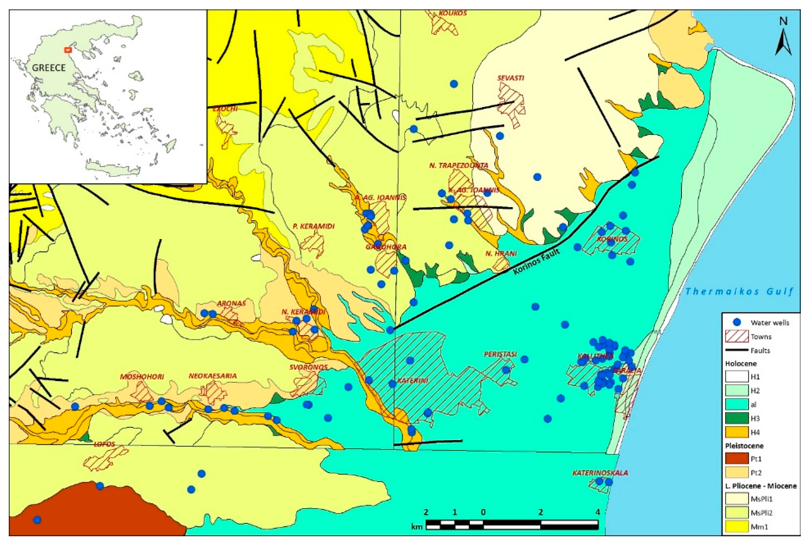
Figure 2.
Hydrogeological map, modified from [25,26]. See text for description of hydrogeological units.
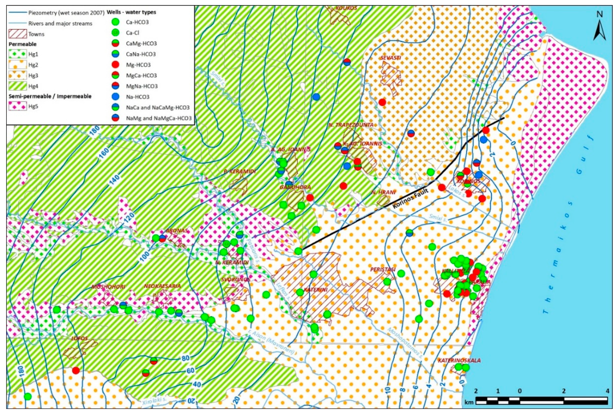
Figure 3.
Heat map of Pearson correlation coefficients (r) for the measured parameters. The first (upper) values of each cell denote the “r” and the second (lower) the p-value.
Figure 3.
Heat map of Pearson correlation coefficients (r) for the measured parameters. The first (upper) values of each cell denote the “r” and the second (lower) the p-value.
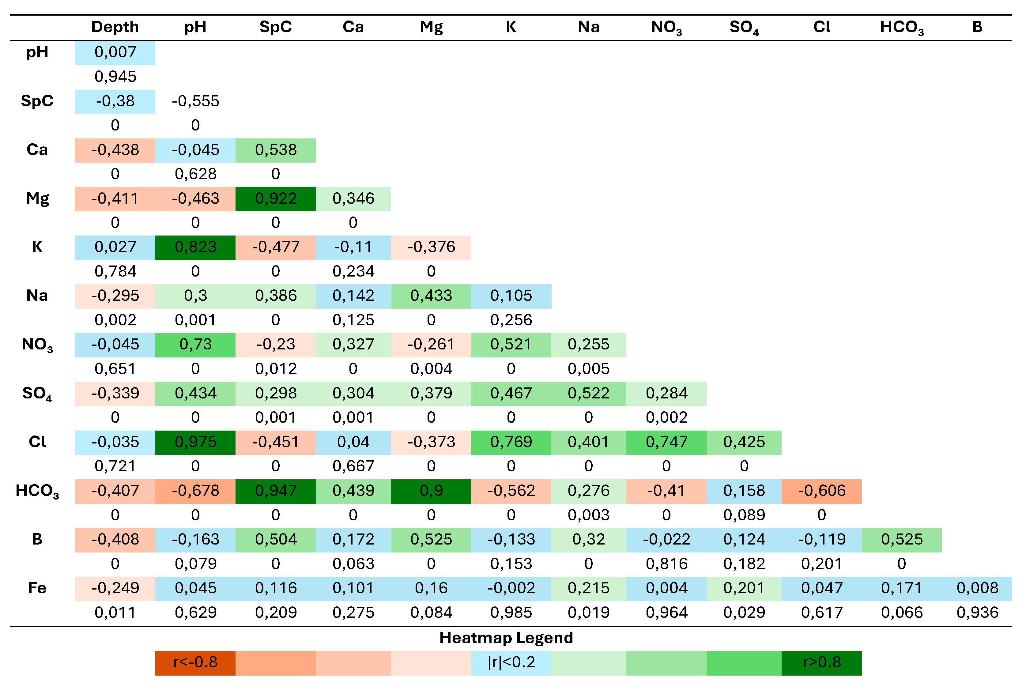
Figure 4.
Dendrogram of Q mode Hierarchical Cluster Analysis (QmHCA) for the groundwater samples. Four groups (A, B, C, D) are identified.
Figure 4.
Dendrogram of Q mode Hierarchical Cluster Analysis (QmHCA) for the groundwater samples. Four groups (A, B, C, D) are identified.
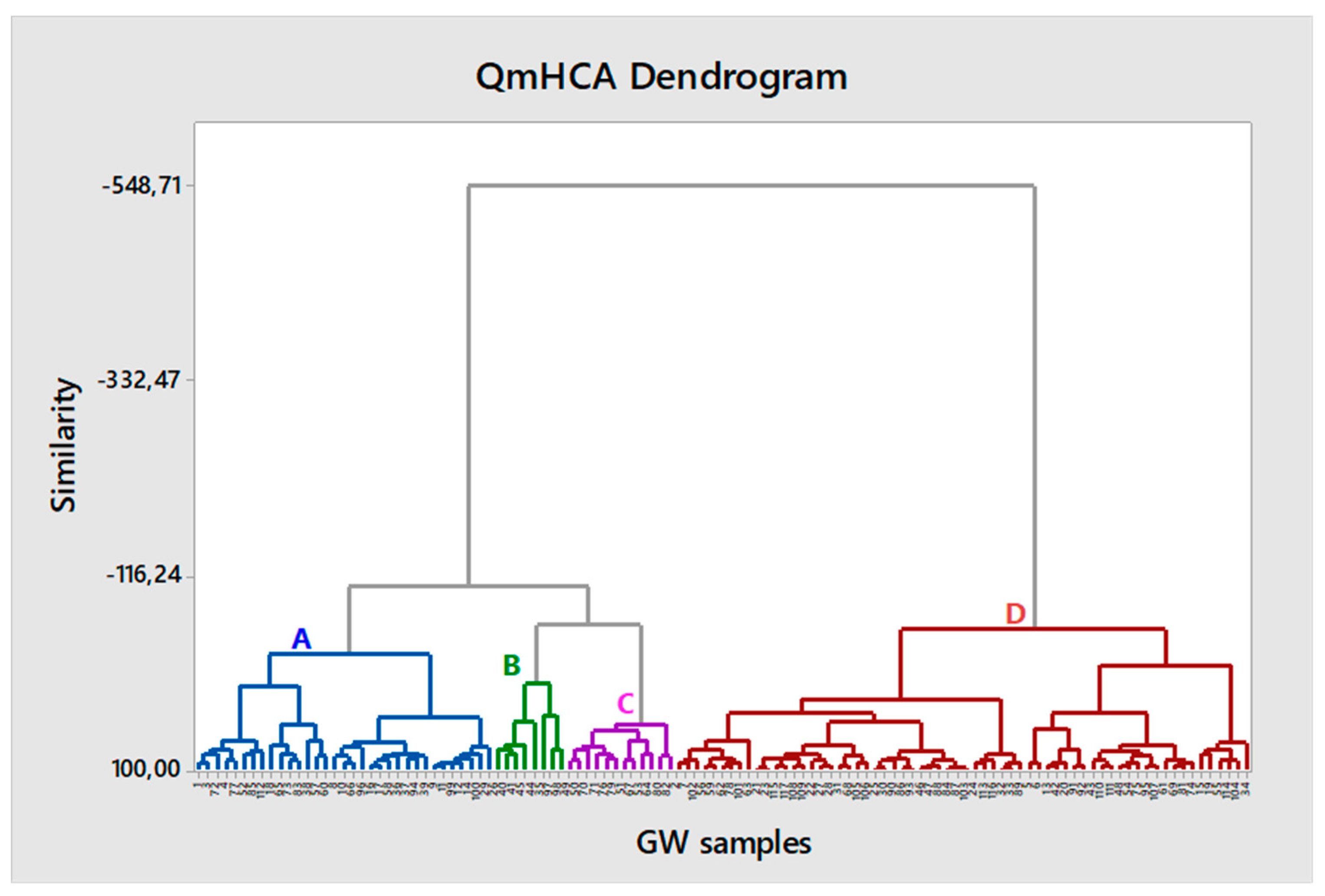
Figure 5.
Dendrogram of R mode Hierarchical Cluster Analysis (RmHCA) for the groundwater samples. Four groups (I, II, III, IV) are identified.
Figure 5.
Dendrogram of R mode Hierarchical Cluster Analysis (RmHCA) for the groundwater samples. Four groups (I, II, III, IV) are identified.
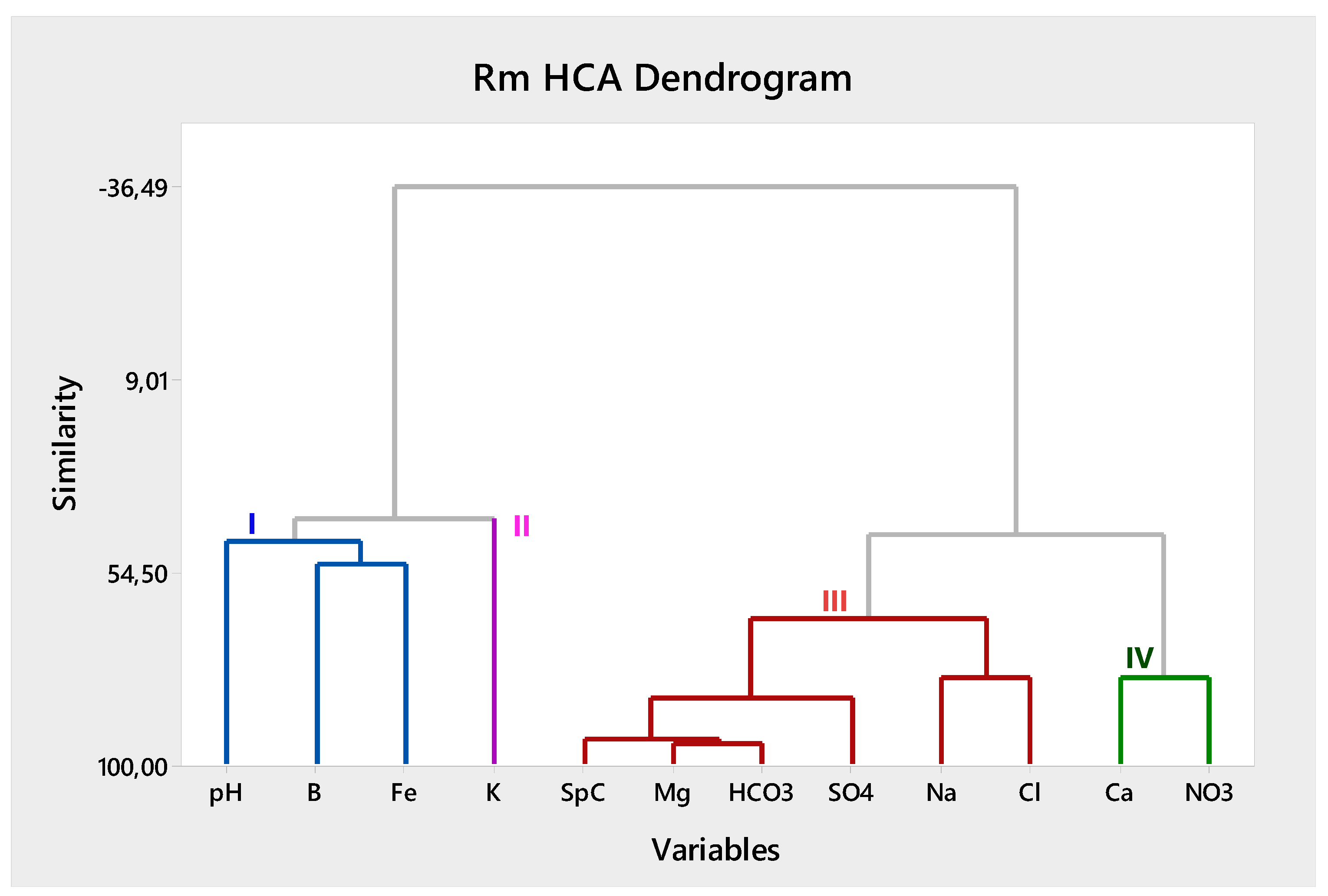
Figure 6.
Spatial distribution of QmHCA groups of groundwater samples and division of hydrochemical well units. The Digital Terrain Model used is from [53].
Figure 6.
Spatial distribution of QmHCA groups of groundwater samples and division of hydrochemical well units. The Digital Terrain Model used is from [53].
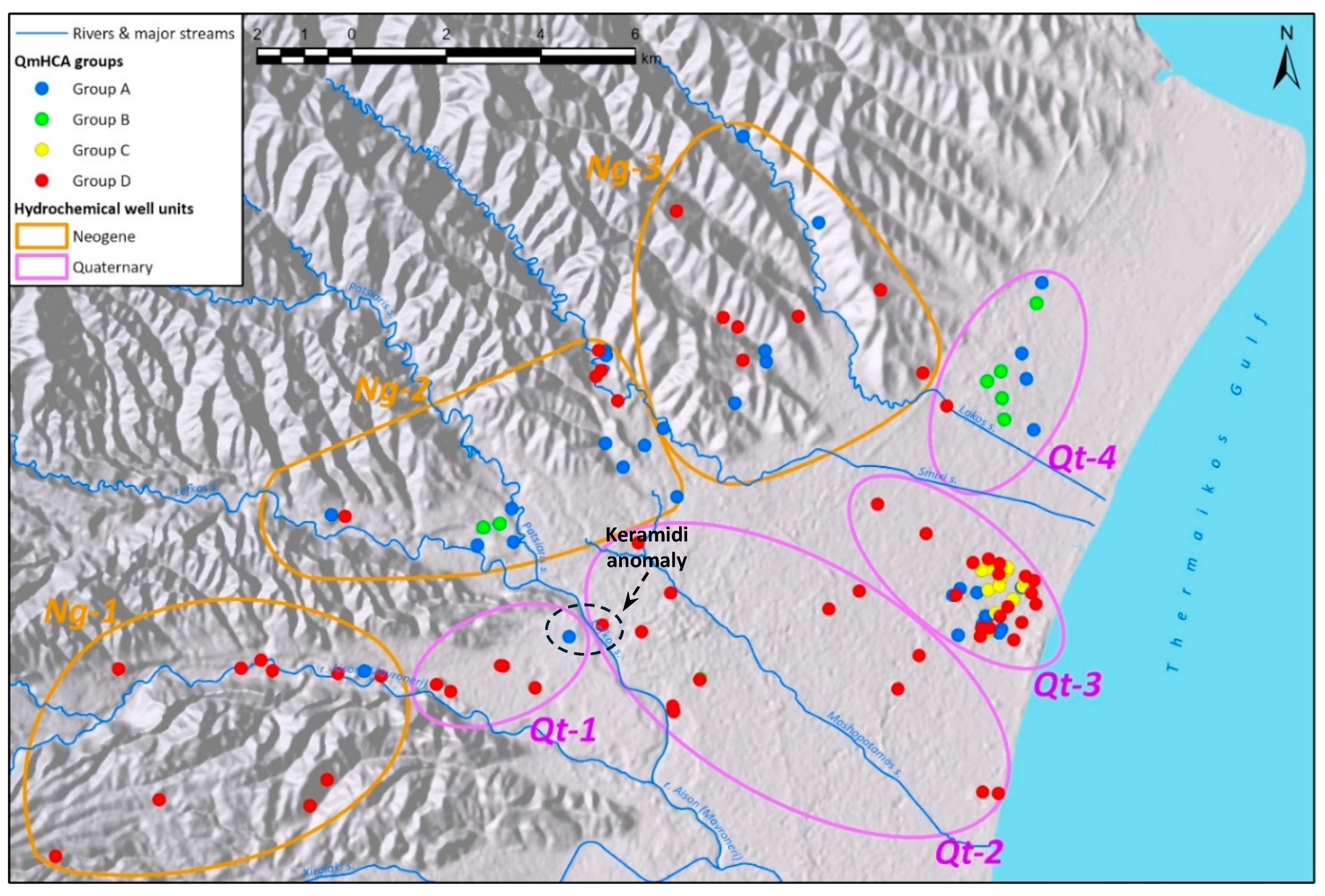
Figure 7.
Piper diagrams depicting the variation of SpC and median water compositions from water wells in the Quaternary of the Katerini plain.
Figure 7.
Piper diagrams depicting the variation of SpC and median water compositions from water wells in the Quaternary of the Katerini plain.
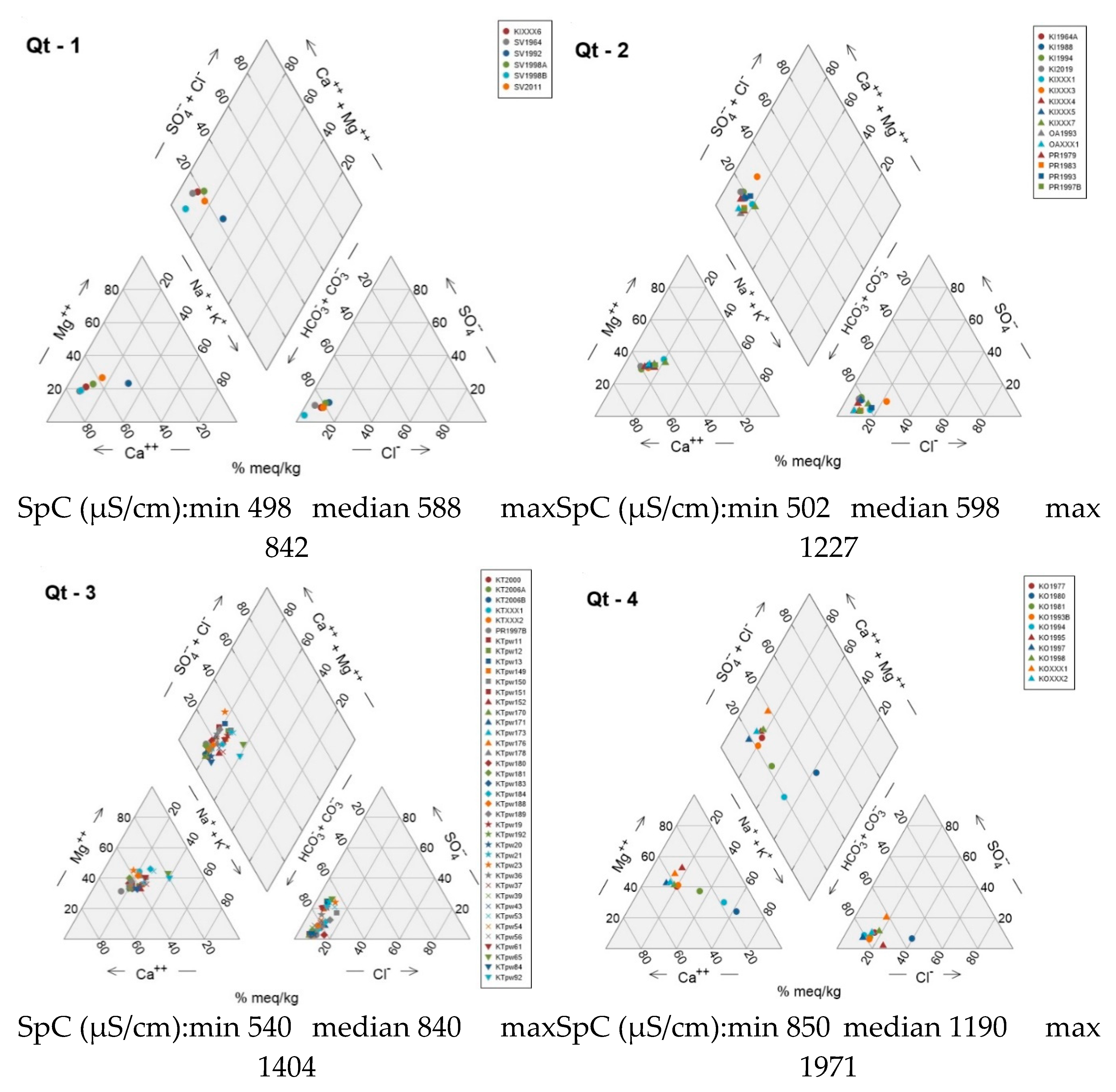
Figure 8.
Piper diagrams depicting the variation of median water compositions from unit Qt-3.(a) shallow water wells (depth ≤ 50 m) and (b) deep water wells (depth > 50 m).
Figure 8.
Piper diagrams depicting the variation of median water compositions from unit Qt-3.(a) shallow water wells (depth ≤ 50 m) and (b) deep water wells (depth > 50 m).
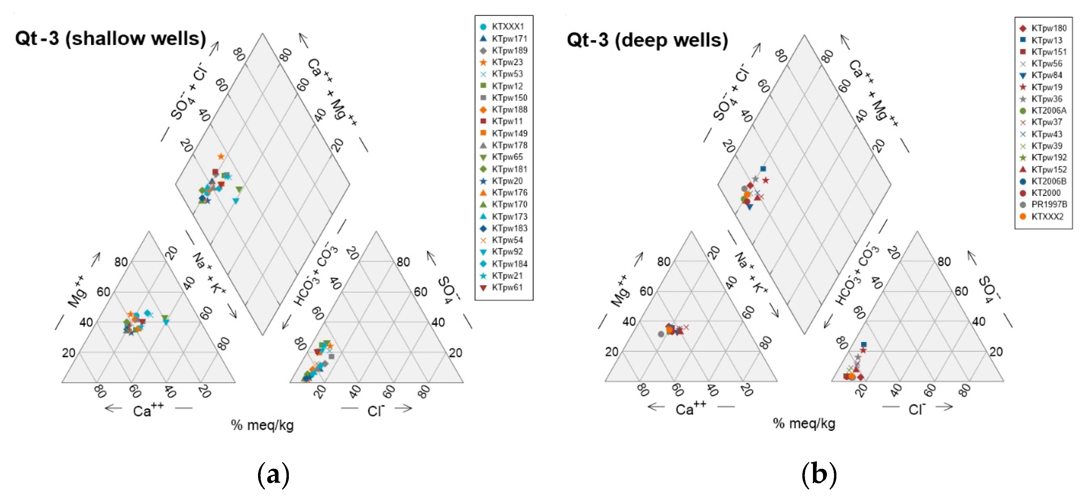
Figure 9.
Piper diagrams depicting the variation of SpC and median water compositions from water wells in Neogene formations.
Figure 9.
Piper diagrams depicting the variation of SpC and median water compositions from water wells in Neogene formations.
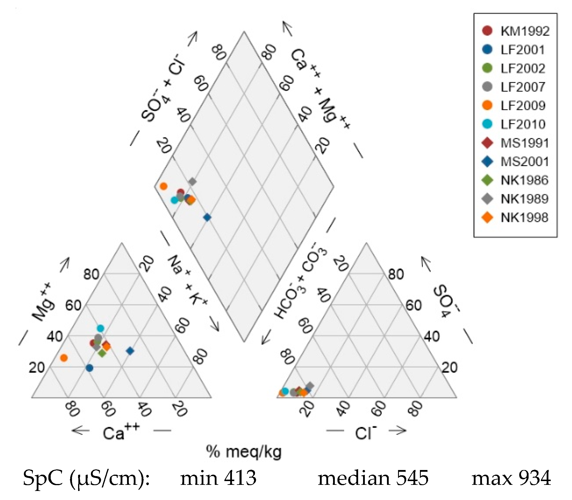
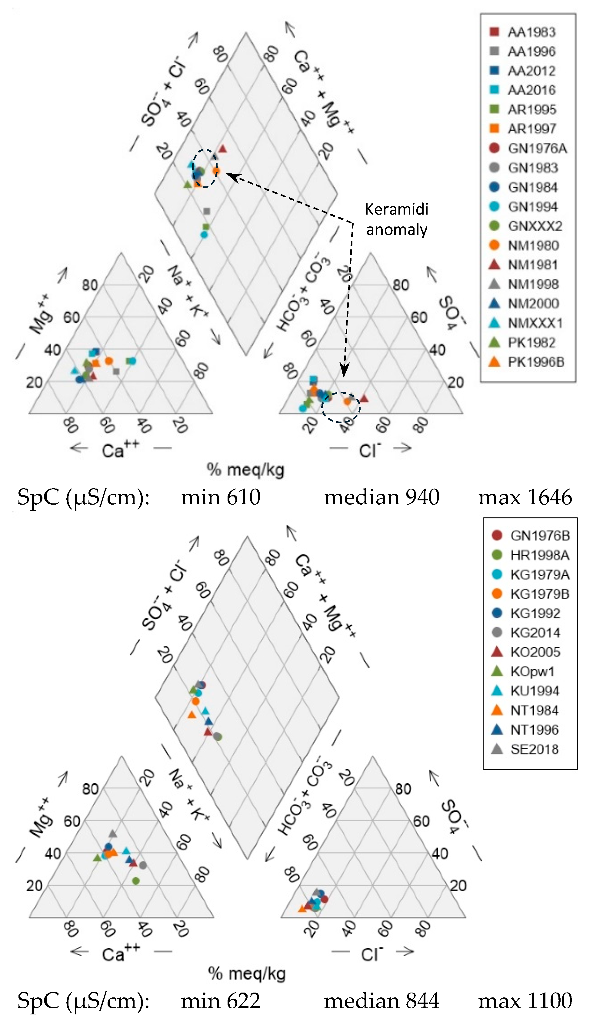
Figure 10.
Piper diagram based on the groundwater sample classification of the QmHCA analysis. (group A: ●, group B: ●, group C: ●, group D ●).
Figure 10.
Piper diagram based on the groundwater sample classification of the QmHCA analysis. (group A: ●, group B: ●, group C: ●, group D ●).
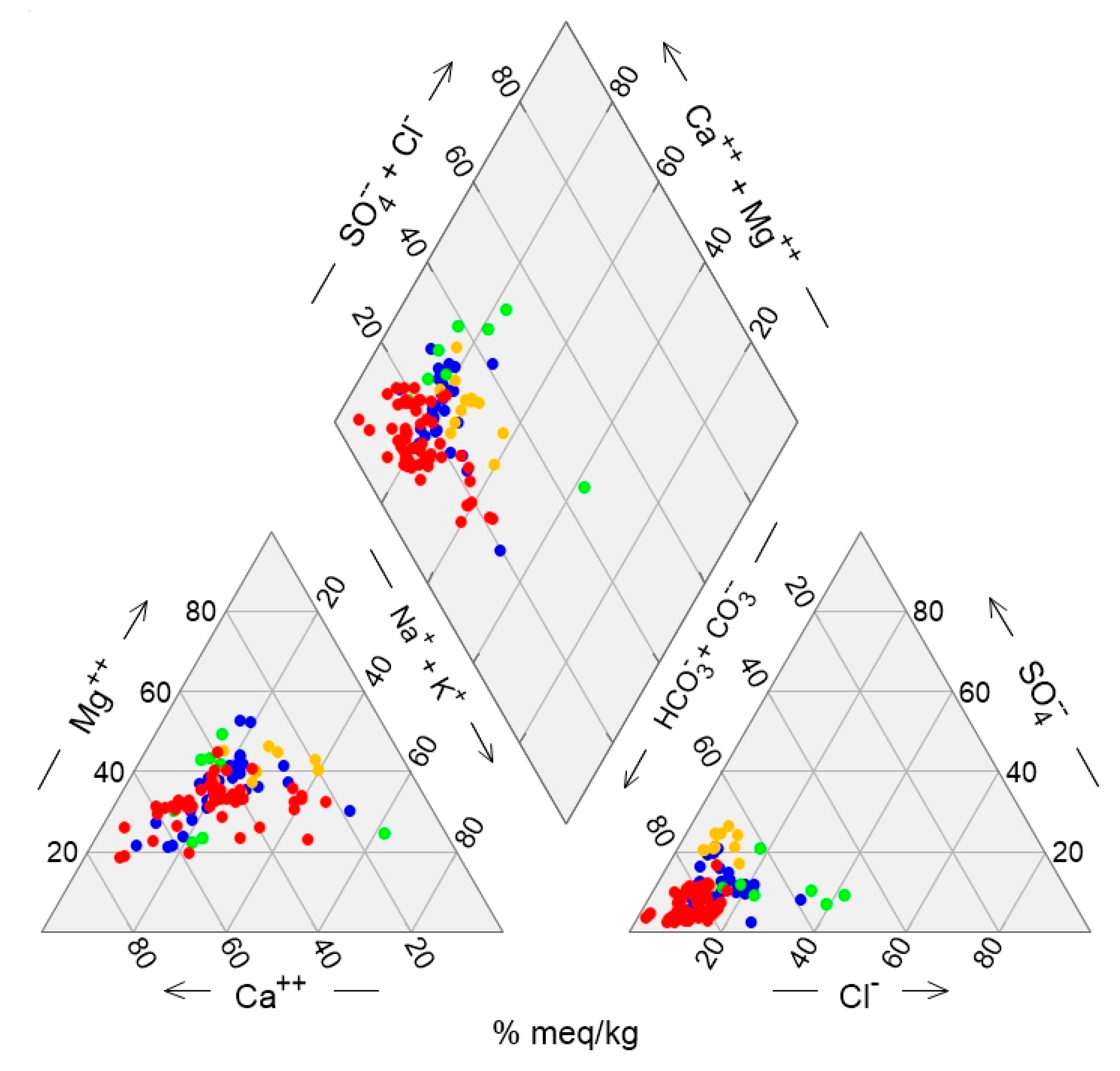
Figure 11.
Bivariate plot of Ca vs Mg for water wells per group of QmHCA. The trendlines illustrated correspond to the limits set in [57]: Mg/Ca>0.9 siliceous aquifers, 0.9>Mg/Ca>0.7 dolomitic aquifers, 0.7>Mg/Ca>0.5 limestone aquifers.
Figure 11.
Bivariate plot of Ca vs Mg for water wells per group of QmHCA. The trendlines illustrated correspond to the limits set in [57]: Mg/Ca>0.9 siliceous aquifers, 0.9>Mg/Ca>0.7 dolomitic aquifers, 0.7>Mg/Ca>0.5 limestone aquifers.
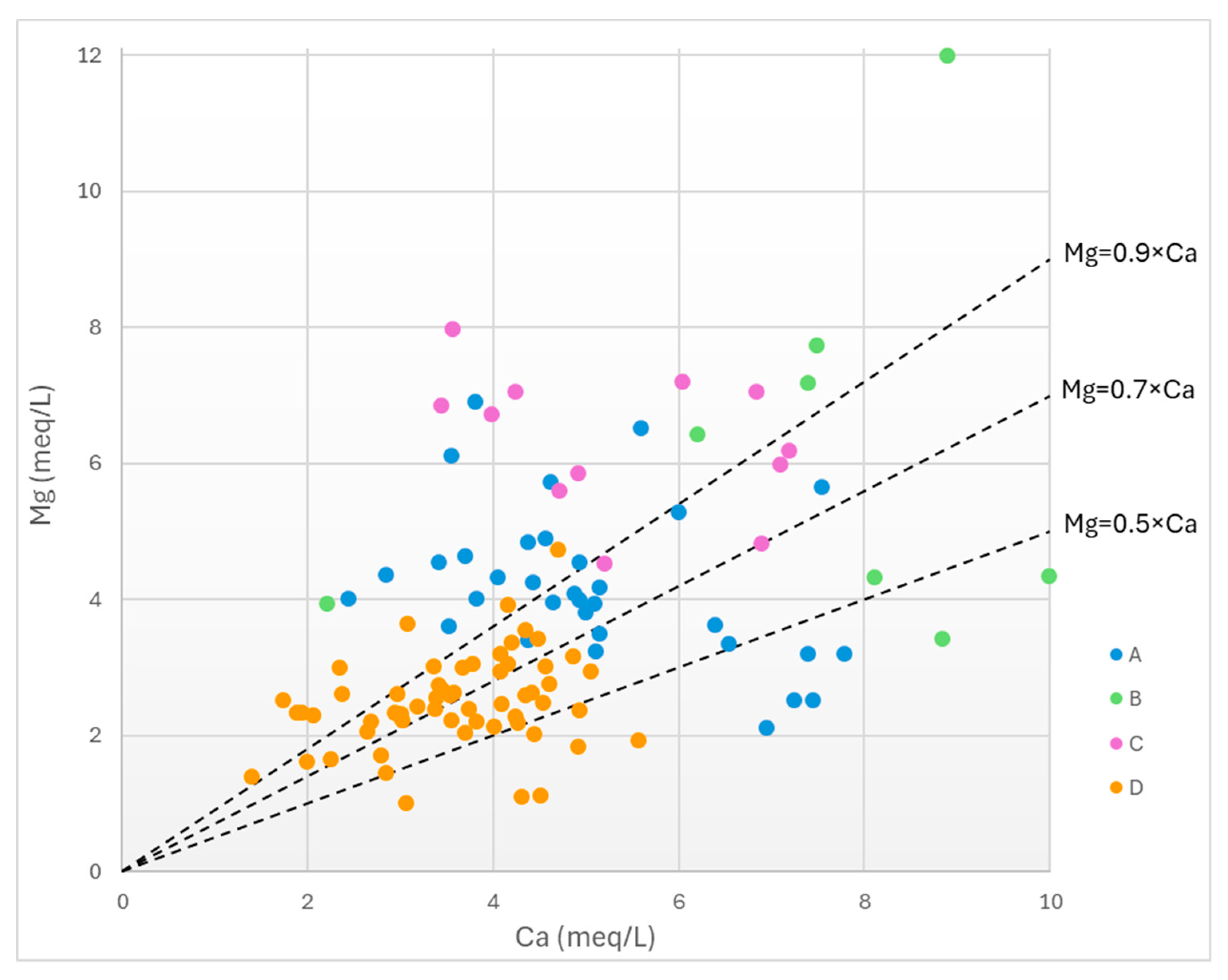
Figure 12.
Bivariate plot of (Ca+Mg) vs (Na+K) for water wells per group of QmHCA.
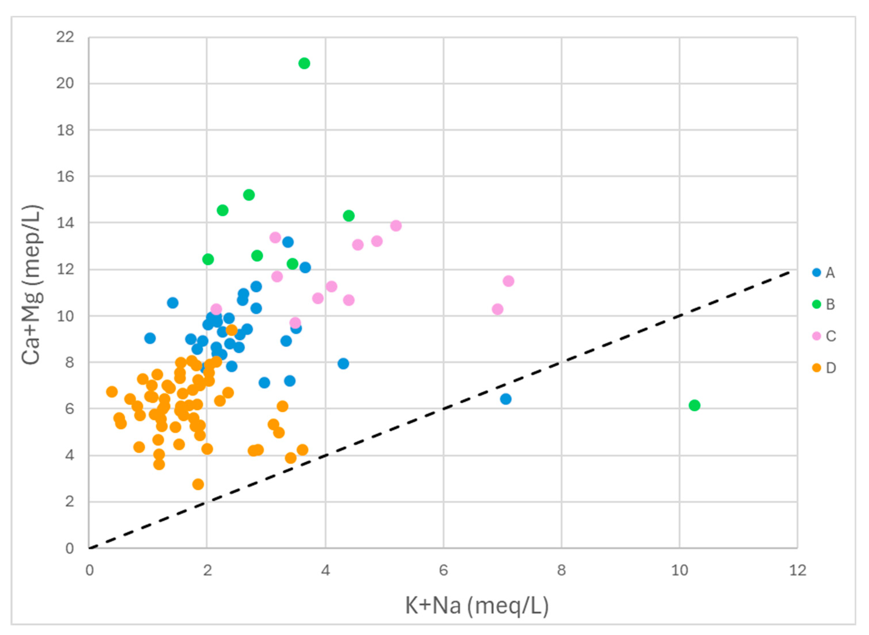
Figure 13.
Bivariate plot of (Ca+Mg) vs (HCO₃+SO₄) (Datta & Tyagi diagram, [59]) for water wells per group of QmHCA.
Figure 13.
Bivariate plot of (Ca+Mg) vs (HCO₃+SO₄) (Datta & Tyagi diagram, [59]) for water wells per group of QmHCA.
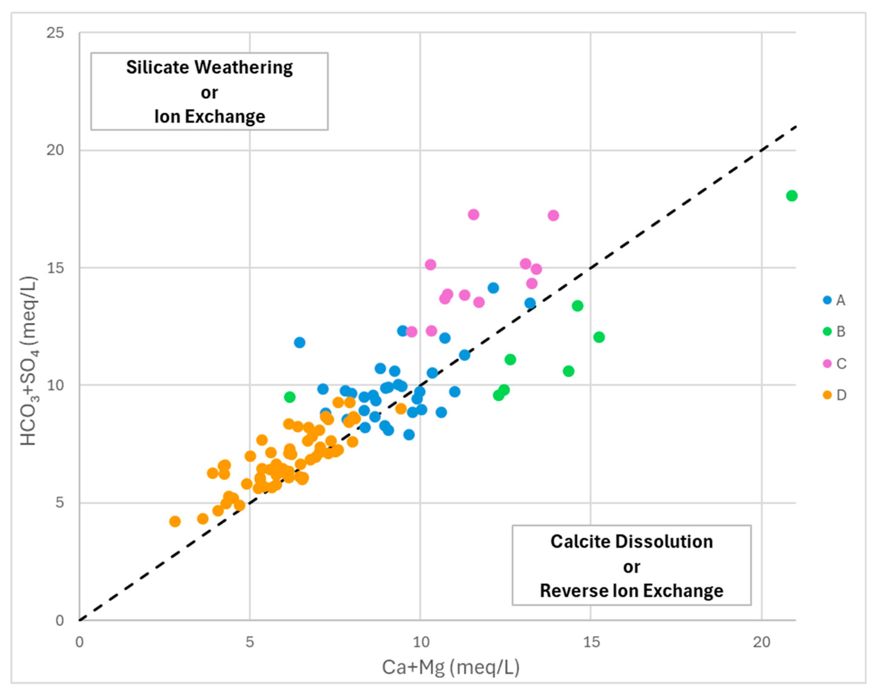
Figure 14.
Bivariate plot of CAI-I vs CAI-II for water wells per group of QmHCA.
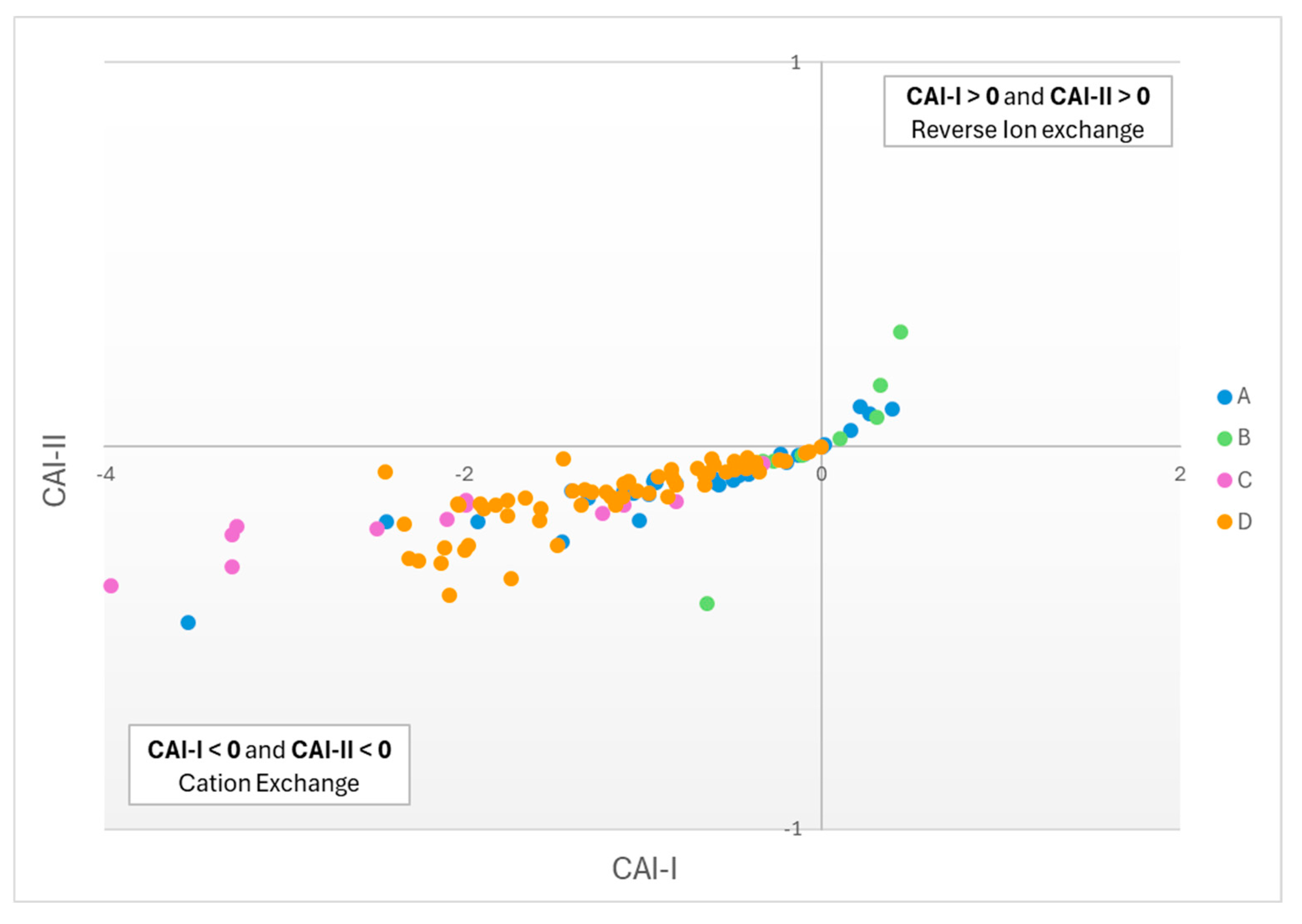

Table 1.
Descriptive statistics for the parameters measured/analyzed in all water wells (2010-2020).
Table 1.
Descriptive statistics for the parameters measured/analyzed in all water wells (2010-2020).
| pH | SpC | Ca | Mg | K | Na | NO₃ | SO₄ | Cl | HCO₃ | B | Fe | |
|---|---|---|---|---|---|---|---|---|---|---|---|---|
| μS/cm | mg/L | mg/L | mg/L | mg/L | mg/L | mg/L | mg/L | mg/L | mg/L | mg/L | ||
| min | 7.3 | 241 | 20 | 11 | 0.3 | 6.9 | 1 | 11 | 6 | 137 | 0.03 | 0.01 |
| med | 7.8 | 775 | 85 | 37 | 1.7 | 45 | 8 | 35 | 36 | 464 | 0.05 | 0.01 |
| max | 8.6 | 1971 | 200 | 146 | 7.3 | 234 | 171 | 239 | 275 | 830 | 0.5 | 1.16 |
| st.dev | 0.2 | 296 | 34 | 22 | 1 | 34 | 27 | 50 | 39 | 132 | 0.08 | 0.16 |
Table 2.
Descriptive statistics for the 4 groups identified by the QmHCA. SpC values are in μS/cm and species concentrations in mg/L.
Table 2.
Descriptive statistics for the 4 groups identified by the QmHCA. SpC values are in μS/cm and species concentrations in mg/L.
| group | pH | SpC | Ca | Mg | K | Na | NO₃ | SO₄ | Cl | HCO₃ | B | Fe | |
|---|---|---|---|---|---|---|---|---|---|---|---|---|---|
| A | min | 7.3 | 750 | 49 | 25.85 | 1.2 | 23 | 1 | 11 | 29 | 448 | 0.03 | 0.006 |
| max | 8.2 | 1292 | 156 | 84 | 7.3 | 160 | 71 | 122 | 149 | 778 | 0.50 | 0.192 | |
| med | 7.7 | 970 | 99 | 49 | 2.2 | 54 | 21 | 61 | 57 | 506 | 0.05 | 0.01 | |
| Β | min | 7.4 | 1227 | 44 | 41.8 | 1.2 | 45 | 16 | 49 | 60 | 495 | 0.03 | 0.006 |
| max | 8.1 | 1971 | 200 | 146 | 2.8 | 234 | 171 | 216 | 275 | 830 | 0.37 | 0.05 | |
| med | 7.4 | 1366 | 156 | 66 | 1.7 | 71 | 94 | 72 | 123 | 565 | 0.11 | 0.01 | |
| C | min | 7.6 | 1017 | 69 | 55 | 0.3 | 49 | 1 | 86 | 32 | 549 | 0.05 | 0.006 |
| max | 8 | 1404 | 144 | 97 | 3.3 | 162 | 47 | 239 | 95 | 775 | 0.43 | 0.668 | |
| med | 7.8 | 1216 | 101 | 79 | 1.4 | 97 | 4 | 159 | 51 | 694 | 0.09 | 0.16 | |
| D | min | 7.4 | 413 | 28 | 12 | 0.3 | 8 | 1 | 11 | 6 | 244 | 0.03 | 0.006 |
| max | 8.6 | 949 | 112 | 58 | 2.8 | 82 | 47 | 76 | 63 | 552 | 0.19 | 1.161 | |
| med | 7.8 | 642 | 73 | 30 | 1.7 | 35 | 7 | 11 | 26 | 387 | 0.03 | 0.006 |
Table 3.
Water wells with median NO₃ concentrations exceeding 40 mg/L.
| QmHCA Group | Well | Median NO₃ (mg/L) | Town | Remarks on land use |
|---|---|---|---|---|
| B | KOXXX2 | 171 | Korinos | inside residential area |
| B | KOXXX1 | 145 | Korinos | agricultural area, edge of residential area |
| B | KIXXX3 | 106.5 | Katerini | sports complex, inside residential area |
| B | KO1997 | 98.1 | Korinos | football pitch, inside residential area |
| B | KO1998 | 90.6 | Korinos | football pitch, inside residential area |
| A | KIXXX6 | 70.75 | Katerini | football pitch, edge of residential area |
| A | GNXXX2 | 60.7 | Ganohora | agricultural area, urban waste management |
| A | NK1989 | 55.1 | Neokaesaria | near residential area, proximity to cemetery |
| A | KG1992 | 47.8 | Kato Ag. Ioannis | inside residential area, proximity to cemetery |
| C | KTpw150 | 46.7 | Kallithea | agricultural area, edge of residential area |
| D | KI1964A | 46.5 | Katerini | inside residential area |
| A | KTpw171 | 46.3 | Kallithea | agricultural area, edge of residential area |
| D | KO1977 | 43.1 | Korinos | agricultural area, edge of residential area |
| D | KI1994 | 40.2 | Katerini | sports complex, inside residential area |
Disclaimer/Publisher’s Note: The statements, opinions and data contained in all publications are solely those of the individual author(s) and contributor(s) and not of MDPI and/or the editor(s). MDPI and/or the editor(s) disclaim responsibility for any injury to people or property resulting from any ideas, methods, instructions or products referred to in the content. |
© 2024 by the authors. Licensee MDPI, Basel, Switzerland. This article is an open access article distributed under the terms and conditions of the Creative Commons Attribution (CC BY) license (http://creativecommons.org/licenses/by/4.0/).
Copyright: This open access article is published under a Creative Commons CC BY 4.0 license, which permit the free download, distribution, and reuse, provided that the author and preprint are cited in any reuse.


