Submitted:
02 July 2024
Posted:
03 July 2024
You are already at the latest version
Abstract
This paper presents two novel bio-inspired particle swarm optimisation (PSO) variants: biased eavesdropping PSO (BEPSO) and altruistic heterogeneous PSO (AHPSO). These algorithms are inspired by types of group behaviour found in nature that have not previously been exploited in search algorithms. The primary search behaviour of the BEPSO algorithm is inspired by eavesdropping behaviour observed in nature coupled with a cognitive bias mechanism that enables particles to make decisions on cooperation. The second algorithm, AHPSO, conceptualises particles in the swarm as energy-driven agents with bio-inspired altruistic behaviour which allows the formation of lending-borrowing relationships. The mechanisms underlying these algorithms provide new approaches to maintaining swarm diversity which contributes to preventing premature convergence. The new algorithms were tested on the 30, 50 and 100-dimensional CEC'13, CEC'14 and CEC'17 test suites, and various constrained real-world optimisation problems, against 13 well-known PSO variants and the CEC competition winner, differential evolution algorithm L-SHADE. The experimental results show that both algorithms, BEPSO and AHPSO, provide very competitive performance on the unconstrained test suites and the constrained real-world problems. They were significantly better than most other PSO variant on most problem sets and no other comparator algorithm was significantly better than either of them on any of the 50 and 100-d problem sets.
Keywords:
bio-inspired search algorithm
; optimisation
; particle swarm optimisation
; swarm intelligence
; altruism
; eavesdropping
; group behaviour
; metaheuristics
1. Introduction
In recent years swarm intelligence algorithms have become one of the most widely used class of optimisation methods. Their effectiveness and convenience has led to many variants [1] and successful applications to diverse real-world problems [2,3,4,5]. One of the best known and most widely applied swarm algorithms is particle swarm optimisation (PSO) [6]. The PSO algorithm has been extensively investigated with regards to its search dynamics [7,8] and theoretical strengths and limitations [9,10], resulting in many recent extensions developed with the intention of improving the performance of the canonical PSO [11,12,13,14,15,16].
Despite many variants with diverse inspirations, the core analogy at the heart of most PSO algorithms is biological: a simple model of flocking behaviour observed in many species. Indeed bio-inspiration has become the dominant driving force for many new meta-heuristic algorithms. However, the canonical PSO algorithm’s model of particle movement [6] is relatively simple compared to natural flocking behaviours. Hence, in most cases, the homogeneous nature of canonical PSO particles’ behaviour moves them towards a common goal using two standard exemplars, their ’cognitive’ (own best position) and ’social’ (swarm best position) influences, which tends to trigger rapid loss of diversity, leading to premature convergence. There have been various approaches to addressing this problem over the past decade or so, including: hybridisation with other search algorithms [13,17,18], using extended learning strategies [19,20,21], and employing more sophisticated topologies to define the local population structure [22,23,24,25]. Another powerful contemporary way to potentially minimise this issue, and to improve the balance between exploitation and exploration within the search process, is to design efficient heterogeneous agent behaviours to avoid the stagnation of particles and improve overall performance by avoiding premature convergence [11,14,26].
In light of this, here we propose two novel PSO algorithms that take their inspiration from forms of animal group behaviour that, as far as we know, have not previously been used in search algorithms: altruism and eavesdropping. These analogies are used to develop algorithms that possess heterogeneous behavioural dynamics at both agent and swarm level. Through this heterogeneity more efficient exploration and exploitation search dynamics are enabled, while maintaining diversity and avoiding premature convergence. Such effective exploration and exploitation performance is especially important for efficient search of high-dimensional and complex problem spaces, which feeds into our overall motivation: the development of powerful new general-purpose optimisers for unconstrained and constrained single objective real-valued problems.
The performance of the new algorithms, biased eavesdropping PSO (BEPSO) and altruistic heterogeneous PSO (AHPSO), was verified over multiple dimensions of the widely used CEC’13, CEC’14 and CEC’17 benchmark test suites, along with various constrained real-world problems, compared against 13 well known state-of-the-art PSO variants and the 2014 CEC competition winner, L-SHADE (a powerful differential evolution algorithm). The overall results of this thorough comparative investigation show that both BEPSO and AHPSO are superior to most of the comparator algorithms and highly competitive against all others on high-dimensional complex problems (none of the other algorithms were statistically superior to the new algorithms on such problems). In addition they are shown to be very strong candidates for real-world applications. Both algorithms provide robust high quality performance across a wide range of test problems and suites with a single set of parameter values; they did not need tuning for each new type of problem.
2. Background
2.1. Particle Swarm Optimisation
In the canonical PSO [6], particles represent a solution in a D-dimensional search space, and each particle possesses three attributes: its position, memory of its best position so far, and a velocity; denoted by the vectors , and , respectively. Initially, each particle’s velocity and position are randomly assigned, and subsequently, at each time step, the fitness function is employed to guide particles towards a combination of and , the best position known to the swarm at time t. At each time step, the velocity and position of each particle is updated using the following two equations:
where is an inertial weight parameter that reflects the impact of the previous velocity on the new velocity and is an important factor in achieving a balance between global exploration and local exploitation. In addition, and are the `cognitive’ and `social’ acceleration coefficients, where the cognitive coefficient controls the local search (guided by ) whilst the social component controls global exploration (guided by ) and represents a kind of cooperation between the particles. The control of these two coefficients is important in performing efficient search as too high values of would lead to excessive wandering of the particles and, similarly, a too high value of would lead to premature convergence of the swarm. and are random D-dimensional vectors with each component generated in the range , powering the stochastic element of the search.
The novel search algorithms introduced in the next section build upon this basic framework.
2.2. Eavesdropping Behaviour in Animals
Eavesdropping plays a significant role in animal communication, and the evolution of such communication [27]. Briefly, eavesdropping occurs as a result of animals accessing communication signals, transmitted by heterospecifics (of a different species or group), that were not intended for them. In nature, it is more common for signal interceptors to be intraspecific (of the same species) in order to perceive the call and extract the required information accurately. However, it is not uncommon to observe interspecific animals (competitors of a different species) intercept signals and use them as an advantage to increase their own fitness. Interspecific eavesdropping is particularly interesting as different species may be proficient in distinct areas within the same habitat and capable of recognising different threats through their distinct sensory capabilities. A concrete example of interspecies eavesdropping is illustrated by the relationship between red squirrels and Eurasian jays [28]. In this case truly astonishing evolutionary dynamics have resulted in communication between a mammal and a bird, which have become positively biased towards one another and are able to warn and guard each other within the same habitat.
The BEPSO algorithm, detailed in the next section, is inspired by the alert-signalling behaviour of animals used to attract conspecifics (of the same species or group) to a discovered resource location for potential exploitation, and the way in which surrounding heterospecific eavesdropper animals try to exploit that information themselves to improve their own fitness.
2.3. Altruism
The AHPSO algorithm, detailed in the next section, is inspired by a certain kind of altruistic animal group behaviour.
The role of altruism in evolutionary dynamics was first analysed in mathematical detail by W.D. Hamilton in 1964 [29]. He showed how altruism could arise and be maintained within the Darwinian framework, conferring overall benefit to the group if not to the individual. Traditionally, researchers tended to assess the benefit of altruism to an organism by examining the average number of offspring, with contributors exhibiting less reproductive success in comparison to beneficiaries. However, several different types of altruistic behaviours have been discovered in various species. Some exemplary altruistic behaviours are observed in social insect colonies such as ants, wasps, bees and termites. In these colonies, the sterile workers are devoted to the queen by protecting the nest and foraging food. By doing so, sterile workers have no reproduction fitness, but they contribute to the queen’s reproductive efforts. An example of a more complex organism exhibiting altruistic behaviour is the blood regurgitating vampire bat that feeds undernourished bats to avoid starvation in their group [30]. Velvet monkeys exhibit similar behaviour to their groups by giving alarm calls to warn of the presence of predators, in doing so putting themself at risk [31]. The type, level, and results of altruistic behaviour vary widely between organisms, as do the relationships evolved between helper and beneficiary actors.
3. Materials and Methods
In this section the two novel PSO search algorithms, BEPSO and AHPSO, are explained in detail. For both the aim was to design heterogeneous particle behaviours that maintain diversity and provide efficient search.
3.1. BEPSO: biased eavesdropping PSO
In BEPSO the particle’s bio-inspired behaviour model comprises three components: recognition, communication, and bias. The recognition component refers to the particle’s ability to distinguish between conspecific and heterospecific particles. The communication component refers to the implicit signal-based communication particles perform when they discover a new and better position. The bias component enables particles to build a form of perception towards each other that evolves through social experiences. This perception is used to adopt different behaviours during the search process.
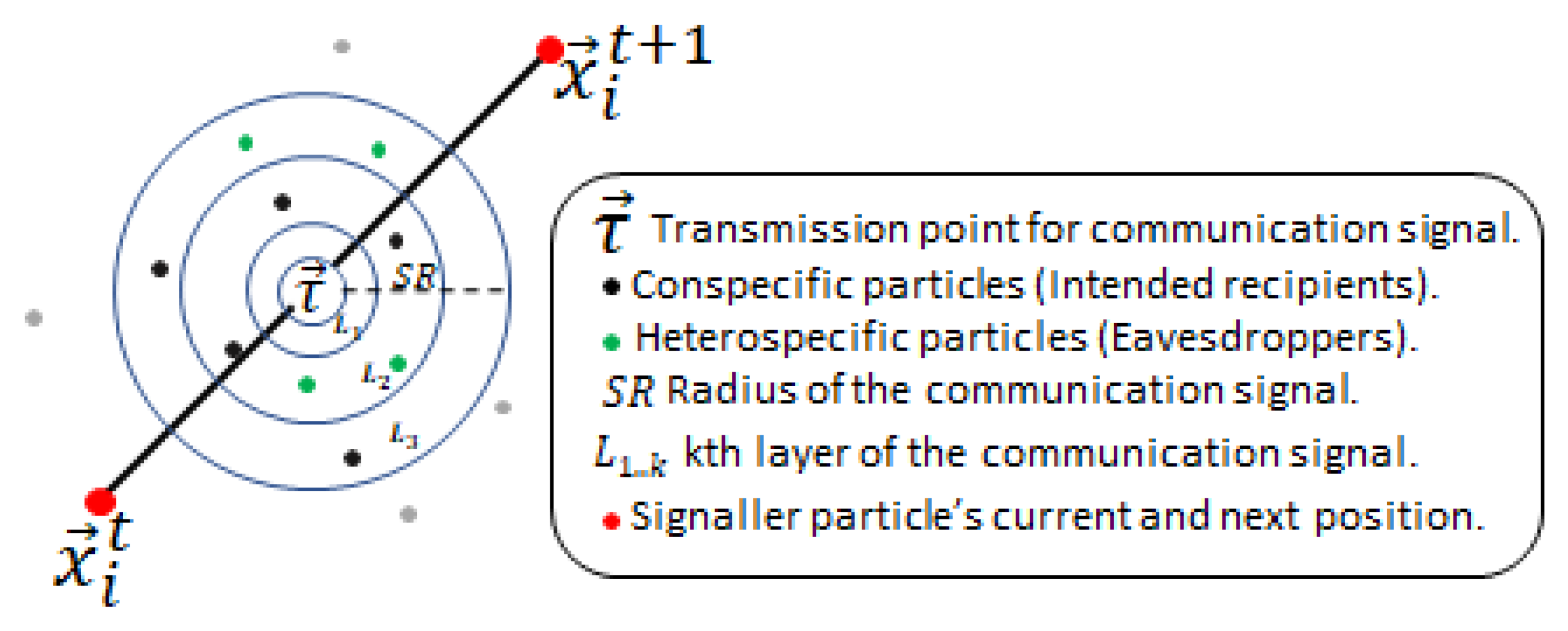
Initially, particles are divided into two groups. Particles of the same group recognise each other as conspecifics, and those from the other group as heterospecific. All particles are assigned an initial random bias towards the rest of the particles in the swarm in such a fashion that any two conspecific particles may be either negatively biased or unbiased towards each other, while any two heterospecifics may be positively biased towards each other. Particles’ search behaviour initiates by updating velocity and position using the canonical PSO algorithm’s update equations (Equations (1)- (2)). After the positional update, if particles discover a better position, in an attempt to guide conspecifics to a potentially better location, the particle communicates with the surrounding conspecific particles by transmitting a signal indicating the new location. The signaller particle intends the communication signal recipients to be solely conspecifics, but surrounding heterospecific particles eavesdrop and exploit the information in the signal (as detailed later). The signal recipients (from both conspecific and heterospecific groups) either accept or reject the information provided by the signal considering several factors, including their bias towards the signaller particle. Before transmitting the signal, the particle determines the transmission point for the intended communication signal. is a position that lies between the previous and the current position of the signaller particle and is calculated using Equation (3).
where and are the current (newly discovered) and previous position of the signaller particle, and is a uniformly distributed random number in the range . The communication signal has a radius defined by the SR parameter with minimum and maximum bounds. and where UB, LB are upper and lower bounds of the given problem and d is the dimension of the problem. The radius of the communication signal is determined individually for each signal based on the particle’s fitness compared to the average fitness in the swarm. This simulates the signal’s loudness; hence, the range of the signal extends or shrinks based on the quality of the discovered position. This behaviour mimics the confidence of the particle in the quality of the discovered location to attract more conspecifics. Hence, a confident signaller particle transmits a signal with a wider influence range, while particles with less confidence in the quality of the discovered position use lower SR with the intention of transmitting a signal to fewer conspecifics, hence minimising potential loss of fitness in the conspecific population. The SR parameter is calculated using Equation (4).
where is the fitness of the signaller particle (to be maximised, in the case of function minimisation this is inversely proportional to the function evaluation value ), is the average fitness in the swarm at time t, and is a random number in the range . This ensures fitter particles shout louder (have higher ). The communication signal is modelled using k signal layers to mimic environmental noise and distortion of the signal as it travels out towards the boundary of the signal range. Hence, recipient particles located in different locations relative to the signal “hear” differently distorted variants of the original signal (newly located position). Figure 1 shows a visual depiction of the communication signal with intended conspecific recipients and eavesdroppers. We mutate the signal vector k times (for k signal layers), with a non-uniform Gaussian mutation operator, starting with a small mutation , and as k increases, increasing the mutation probability to trigger larger mutations. This ensured that the further away a particle is, the more distorted the signal it receives. Any particle whose Euclidian distance from the transmission point is less than is a recipient of the signal (see the algorithm pseudocode).
Particles (both conspecific and eavesdroppers) can accept or ignore the information provided by the communication signal depending on their bias and the signaller particle’s confidence in the newly discovered position (detailed later). The recipient particles closest to the transmission point receive the least distorted signal, and those furthest the most distorted. This set of stochastic mechanisms – distorting the signal as it travels across the search space and placing the transmission point between the current and last location – prevents multiple particles clustering in exactly the same location, while encouraging movement towards confidently signalled better regions, helping to avoid stagnation within recipient particles.
Figure 1.
Visual representation of the communication signal sent by the signaller particle
Among animals, survival and cooperation strongly depends on bias towards others, either through genetic influence, e.g. cooperating with a conspecific for the first time regardless of any lack of previous experience, or through social learning where positive association play a role. In our algorithmic model, particles are either positively biased, negatively biased or neutral (unbiased) towards each other, and use their bias to decide whether to accept or reject the information the signal provides as a guide. Negative bias can be thought of as the particle’s defence mechanism built over time to avert potential negative social guidance and thus minimise loss of fitness due to misleading communication signals. Positive bias, on the other hand, enables particles to form an implicit cooperative relationship and accept guidance through signal calls from established "social partners" formed over time in an attempt to improve fitness. Both mechanisms complement each other and allow particles to form decentralised communication that evolves based on particles’ individual social experiences. Particles’ biases form over time as a result of the accumulation of consecutive positive or negative experiences attained from the use of signal information. The experience is positive when the signal improves the fitness of the recipient particles, and negative when it reduces it. The accumulator decision model from the free-response paradigm [32] is employed to enable particles to accumulate evidence through signaller-recipient relationships. When either of the two accumulated experience variables ( (positive) and (negative), Equation (5)- (6)), reaches a threshold, a decision response is triggered, to accept or reject a signal. The following update equations are used to build the bias “evidence” between a recipient and a signaller particle (assuming minimisation of the fitness function, ):
where is the positive and is the negative bias response variable at time t that the particle (recipient) has collected for the particle (signaller), and is the accumulating factor that contributes towards the bias response variables:
If the experience is positive, increases, if it is negative decreases.
Figure 2 shows the visual depiction of Equations (5)-(6) unfolding over time. Each time evidence is collected, Equation (8) is used to determine if either of the response variables, and , has reached the specified bias threshold values (the threshold is positive, the threshold is negative).
where is the particle’s bias towards the particle, the threshold, , is an integer in the range [10, 100]. The value of controls the pace at which particles become biased; hence the value of can have a direct impact on the behaviour of particles. Particles tend to be rapidly biased when is set in the lower range. On the contrary, particles can remain unbiased towards most other particles in the swarm for extended periods when is in the higher range.
At the beginning of the search process, all particles are given random biases; positive (1), negative () or neutral (0), to allow heterogeneity from the start of the search process. Since there would be no transmission of signals at , all particles initially update their velocity and position using the standard PSO update equations Equations (1)-(2)). After the positional update, if the particle discovers a better position, it must transmit a communication signal to attract conspecifics to a potentially better location using the procedures described above.
To try and avoid costly `mistakes’ due to misleading information, receiving particles, both conspecifics and surrounding eavesdropping heterospecifics, decide to exploit or ignore the signal information by a simple risk versus reward assessment. The following rules define the criteria both conspecifics and eavesdroppers use to exploit or ignore the signal information:
- Conspecific recipient particles decide to exploit signal information only if the recipient particle is positively biased or unbiased towards the signaller, and the signaller particle’s confidence in the newly discovered position is high.
- Eavesdropper particles decide to exploit signal information if the eavesdropper is positively or negatively biased towards the signaller, but the signaller’s confidence in the newly discovered position is high.
The signaller particle’s confidence is high if and is low if .
In nature, animals adopt various strategies to deter eavesdroppers or makes their signals less desirable or noticeable to heterospecifics. In this study, the signaller particle aims to evade eavesdroppers by adopting a probabilistic strategy whereby it occasionally deliberately uses a smaller values to attract fewer particles (see algorithm psuedocode for details). This behaviour enables signallers to appear less confident in the quality of the discovered position to make the signal less conspicuous for eavesdroppers. This evasion strategy mostly affects eavesdroppers, even whilst negatively biased towards the signaller particle, because they place weight on the signaller’s confidence. However, it comes at a cost to conspecifics of the signaller as it narrows the range, meaning fewer receive the signal.
Both conspecific and eavesdropper recipients that adopt the signal-based guidance use the following equation to update their velocity:
where is the signal vector for the layer of the signal (the appropriate layer relative to distance between signaller and recipient), and the other symbols are as used previously in Equation (1).
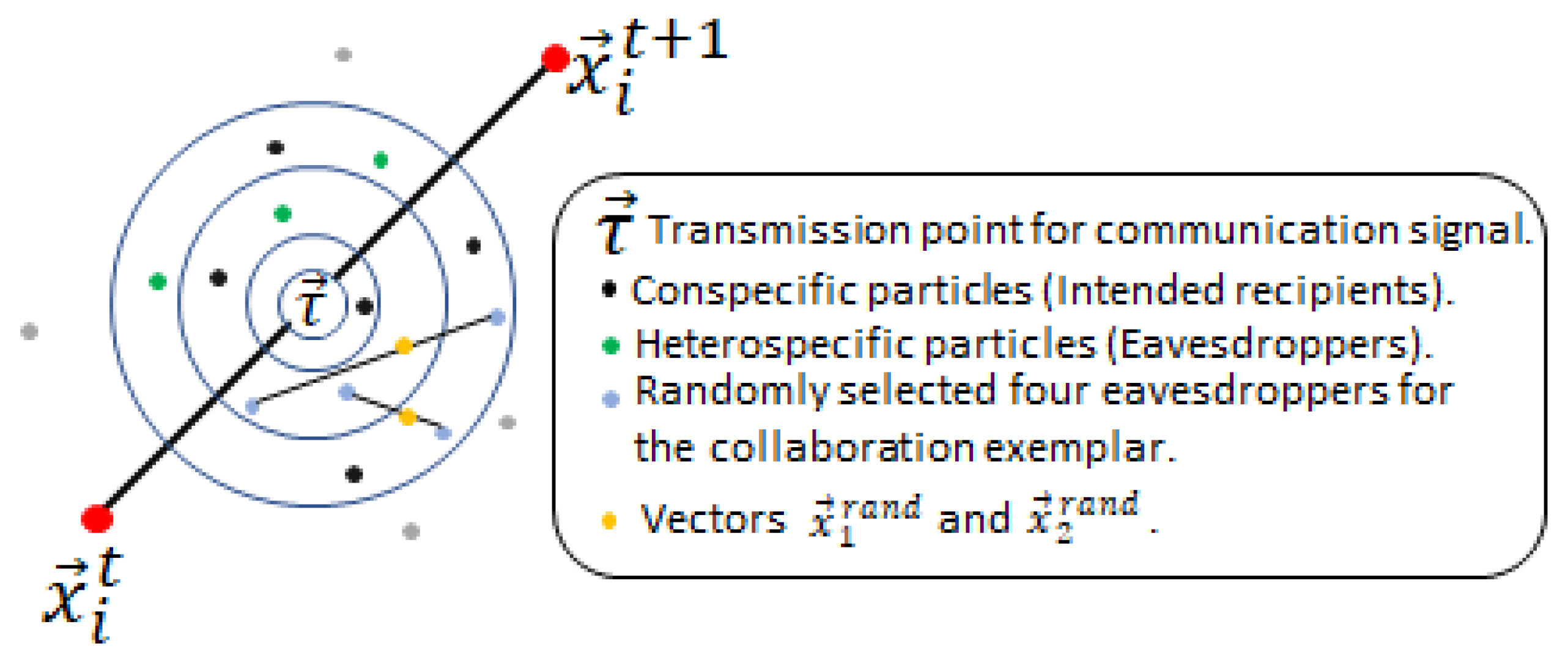
The non-signal based behaviour uses two repellent and a collaboration exemplar. The two repellent exemplars and are the furthest located particle to the signaller and a (randomly selected) non-recipient particle that is outside of the signal range. The two repellent exemplars are selected from the recipient’s conspecific group. The collaboration exemplar requires randomly selecting four recipients from the other group (eavesdroppers). It is calculated as shown in Equation (10).
where – are the four randomly selected eavesdropper particles within the signal range. is a vector that lies between the positions of the first and second selected recipient particles and similarly lies between the third and fourth selected recipients, as illustrated in Figure 3. is the average of the two vectors.
Particles that adopt the non-signal based guidance update their velocities using the following equation:
where is an exemplar randomly selected as either , or .
Imitation is one of the most common social learning behaviours animals adopt. In our algorithmic model, the unbiased recipients imitate the dominating behaviour of their conspecifics. Hence, if p particles of the conspecifics or eavesdroppers adopt the signal-based guidance while q of them adopt the non-signal based guidance, and , then the unbiased conspecific/eavesdroppers imitate the behaviour dominantly adopted by their conspecifics. When , or unbiased particles dominate one or both groups, signal-based or non-signal based behaviour is randomly adopted by the unbiased recipient particles.
Figure 3.
Visual depiction of the particles selected for the collaboration exemplar
The heterogeneity in the swarm is formed by the mix of signal-based and non-signal based behaviour adopted by recipient particles. The particles’ biases formed over time maintains the balance of particles adopting these behaviours. The entitlement of particles as recipients depends on several factors, including the previous and the discovered position by the signaller, the value, and the calculated transmission point. Hence, a small fluctuation to one of these factors significantly alters the list of potential recipients of both conspecific and eavesdroppers at time t. Consequently, which set of particles become recipients is unpredictable for each transmitted signal. This unpredictable yet self-organising behaviour is a further support for population diversity, minimising the risk of particles being stuck at local optima.
In order to fully exploit existing potential solutions, the BEPSO model also incorporates the periodic use of multi-swarms, introduced in the study [26]. Every so often the swarm is split into multiple swarms which support another phase of search, after which they join back together, the standard BEOPSO mechanisms resume, and the cycle repeats.
The initiation of the multi-swarm mechanism requires the division of the swarm into N subswarms. Instead of randomly splitting the swarm into N equal subswarms, in our method, subswarms are formed based on particles’ dominating biases to enable each subswarm to possess an asymmetrical and self-regulating population. Hence, a particle is a member of if it is predominantly positively biased towards most particles in the swarm. Similarly, if a particle is mostly negatively biased or unbiased, then the particle belongs to the corresponding groups and . Each member of a subswarm uses the following equation to update their velocity:
where is the position of the fittest particle in the subswarm.
In summary, particles’ bias built over time ensures behavioural heterogeneity by forcing particles to dynamically adopt signal-based and non-signal based guidance. This primary search strategy is supported by periodically activated subswarm searches to efficiently exploit the existing solutions. The asymmetrical populations in the subswarms exploit different local solutions with varying densities of particles at different search phases, resulting in an efficient search behaviour with a good balance of exploration and exploitation. The overall BEPSO algorithm is shown in Figure 4.
3.1.1. BEPSO Parameters
The BEPSO algorithm involves a number of parameters, but our intention was to develop a technique that does not need tuning for each new problem it is applied to. Hence after extensive preliminary parameter investigations [33] involving a wide range of problems and problem types and sizes, the following set of parameters were found to be robust and effective and was adopted for all subsequent experiments reported in this paper. Note that, in common with many current PSO algorithms, the momentum term, is adaptive and time-varying, as detailed in Figure 4.
population size = 40; length of the two phases of the search (signalling and multi-swarm), both = 10 iterations; = 0.01; = 0.001; bias threshold = 20, other parameters see Figure 4.
3.2. AHPSO: Altruistic Heterogeneous PSO
In this section we describe our second novel PSO algorithm inspired by a certain kind of altruistic animal behaviour, a direction that has not been explored before.
The AHPSO algorithm incorporates conditional altruistic behaviour and a heterogeneous particle model that delays the loss of population diversity and prevents premature convergence, resulting in a highly effective search algorithm. In our approach, particles are conceptualised as energy-driven entities with two possible states, active and inactive. Particles have a current energy level and an activation threshold and are inclined to be active by maintaining their current energy level above the threshold. The distinction in a particle’s state is used to create a heterogeneous population, and particles’ tendency to become active is aided by lending-borrowing relationships among them. Hence conditional altruistic behaviour is exhibited by particles which lend energy to inactive particles to allow them to change their state. In doing so, helper/lender particles risk downgrading their own state from active to inactive. To minimise the risk of reducing their own fitness, a group of lenders assess the situation of the beneficiary/borrower particle, based on the level of altruistic behaviour it has exhibited, before making a decision on whether or not to lend. In our behavioural model, heterogeneity is attained through altruism and better population diversity through heterogeneity. Hence, these two concepts depend on, feed and maintain each other.
In AHPSO two behaviour models are used. The first is the altruistic particle model, which constitutes the particle’s primary behavioural model. The second, the paired particle model, extends the former to boost population diversity further. They are applied one after the other on each overall cycle of the AHPSO algorithm.
3.3. Altruistic Particle Model (APM)
The activation status of particles is dependent on current energy level, , and activation threshold, . Initially both values are randomly assigned. The concept of activation is employed to determine the type of movement strategy for particles at the individual level and as a result, controls the behavioural heterogeneity in the swarm.
Particles have an inherent tendency to be active; hence particles in the inactive state are expected to borrow energy from other particles when their . The main factor influencing and maintaining the swarm heterogeneity is the particles’ altruistic behaviour. A particle that behaves altruistically by making significant energy contributions to other swarm members is highly unlikely to be rejected when in need of energy itself, and on the contrary, particles that exhibit lower altruistic behaviour are inclined to be rejected.
Persistent borrowing behaviour in a particle over prolonged periods results in a highly unstable lending-borrowing ratio and reduces the altruism value, , of the particle (as the particle consumes a lot more resources than it contributes to the swarm). is calculated according to Equation (13).
where and are the number of times the ith particles lent and borrowed energy, respectively, up to time t. When a particle is unable to activate, it attempts to borrow energy from randomly selected potential lenders, and in order to lend energy, potential lender particles expect energy requesting particle to meet an altruism criterion defined by (Equation (14)).
This criterion is based on the independent probability of two events and . For , the altruism value of the borrower particle is used, and is calculated as
where is the number of particles in the swarm with active status at time t, and N is the population size.
gives a rough measure of the probability that a lender particle will return the lent energy from the swarm. In addition to enforcing altruistic behaviour, the criterion provides a form of altruistic assessment of the lender particles’ probability of returning lent energy.
The potential lender particles use the value described by Equation (16) as the final decision to either lend energy or reject the request of the borrower particle.
where is the average altruism value in the swarm.
If the decision is in favour of the energy requesting particle (i.e. true), an equal amount of energy is borrowed from each lender to compensate the required energy of the borrower particle. This is calculated as
where is the amount of required energy from each lender and is the number of selected lenders. The movement strategy adopted by particles in the altruistic behaviour model is based on the altruistic traits of particles. Particles that are active use the canonical PSO update equation shown in Eqs. (1)– (2), whereas inactive particles who do not meet the criterion , and therefore cannot borrow, use Equation (18) to update their velocity (and position via Equation (2)).
where is the personal best position of the least altruistic particle at time t. In the AHPSO framework, particles who do not meet the criterion are less altruistic at time t hence behave together with similarly less altruist particles. Considering the evolving dynamics of the altruistic model, the least and most altruistic particles fluctuate. Hence guidance towards the least altruistic particle partially enables cooperation through altruism and supports heterogeneity. Energy sharing takes place between the lender particles and the borrower who meets the criterion . As lenders are randomly selected without any criteria, there is a distinct possibility of some lenders not having excess energy to lend. Therefore, after borrowing energy, the borrower particle may still lack sufficient energy to activate. In this case, an exemplar for the particle is generated by the mean position of half of the lender particles and their velocity is updated according to Equation (19).
where is the mean position of the randomly selected lender particles.
As commonly seen in certain PSO variants, in our behavioural model, particles do not explicitly exchange positional information, hence, by using the mean position of a proportion of lender particles, we aim to form an implicit communication between lender-borrower particles.
If, however, the borrower particle succeeds in borrowing sufficient energy to activate, the particle’s velocity is calculated using Equation (20).
where is the personal best position of the most altruistic particle at time t. The particle is guided towards the most altruist particle to form partial cooperation and maintain heterogeneity. An additional stochastic element is introduced by randomly reinitiating and for the entire swarm at specific intervals. The idea behind this is to fluctuate the altruism value of particles and allow less altruistic particles at time t to cooperate, contribute and evolve as an altruistic particle. In contrast, an altruistic particle could “devolve” and exhibit selfish behaviour. As a result, this model allows altruistic and selfish particles to adopt distinct movement strategies that change and adapt depending on the level of a particle’s “evolution”, leading to an adaptive and heterogeneous particle population.
3.4. Paired Particle Model (PPM)
The paired particle model is an extension of the altruistic behaviour model described in the previous section. The purpose of the PPM is to further boost the heterogeneity properties of the algorithm, leading to increased population diversity. The PPM is run after the APM on each overall iteration of AHPSO. A relatively small proportion of the population is used for the paired particle model (see Section 3.5.1 for values) . This model employs two movement strategies for the selected particles, namely, a coupling-based strategy and an opposition-based strategy; each pair randomly selects which to use (see Figure 5). The paired particle model enables particles to randomly form and maintain pair-style bonds similar to the mechanism employed in study [34]. An altruistic particle may abandon its pair if the pair is less altruistic than the swarm’s average.
3.4.1. Coupling-based Strategy
The coupling-based strategy distinguishes pairs as tightly or loosely coupled or neutral, which determines the type of movement strategy. The following rules govern the type of coupling relationship paired particles adopt:
- A pair is tightly coupled, if both particles are active at time t.
- A pair is loosely coupled, if both particles are inactive at time t.
- A pair is neutral, if one particle is active and the other is inactive at time t.
Tightly coupled paired particles tend to have more influence on each other than loosely coupled pairs.Tightly and loosely coupled particles update their velocities using Equation (21) and Equation (22), respectively.
where and are the particle’s pair’s position, and personal best position.
is used as a damping factor to prevent the possibility of particles rapidly oscillating, instead performing small movements in this secondary phase of the search. In essence, the coupling-based strategy empowers particles within the paired behaviour model to influence each other regardless of any distance constraints between pairs. Thereby, clustered particles take small steps towards their pair, depending on the type of coupling relationship formed, causing perturbations in the current position without explicit impact on . However, these fluctuations in particle position subsequently influences the next position of the particle, helping to escape local optima.
3.4.2. Opposition-Based Strategy
The opposition-based movement strategy guides paired particles towards exemplars with opposite features. By guiding both particles of a pair in potentially distinct directions, the strategy aims to maintain diversity within such pairs, and hence within a proportion of the population. In a way, this movement strategy partly compensates for the previous coupling-based strategy where pairs influence each other. The opposition-based strategy aims to slow down the learning between pairs, without destroying it, and delays loss of diversity between them by guiding both in the direction of distinct exemplars. The altruism value of the paired particles is used as the determining factor to distinguish the type of movement a particle performs. Exemplar selection for members of paired particles works as follows. If the particle is more altruistic than its coupled pair, its velocity is updated using Equation (23).
where is randomly selected as either or the position of the most altruistic individual of the most altruistic pair at time t.
But if the particle is less altruist than its pair, its velocity is updated using Equation (24).
where is randomly selected as either or the position of the least altruistic individual of the least altruistic pair at time t.
Since both movement strategies in the paired particle model always result in particles moving, they acts as a stabilising mechanism that enables particles to partially escape from local optima and continue the search process. In both coupling-based and opposition-based learning, the fitness of the exemplar particles is deliberately not considered, this helps to minimise particles clustering around local optima, aiming to maintain diversity and hence guard against premature convergence.
3.5. The Search Process of AHPSO
The overall AHPSO algorithm is shown in Figure 5, note that an adaptive, time varying, momentum term, , is employed. The two phases of AHPSO, executed consecutively on each cycle, namely the altruistic and paired particle models, complement each other. The search process is initiated with the APM during which particles attempt to change their state from inactive to active. Behaviourally, active particles tend to be more focused on exploitation. On the contrary, inactive particles, attempting to borrow energy, are more focused on exploration and are mainly influenced by the most and least altruistic particles at time t. The level of altruistic behaviour exhibited by particles varies a great deal and particles evolve frequently from more to less or less to more altruistic. Hence the different types of particles (active, successful borrowers, unsuccessful borrowers) are guided by highly diverse and fast evolving exemplars enabling efficient search behaviour while maintaining population diversity.
Next, the second, PPM, behaviour model takes over. Unlike the main APM, this is used for only a selected proportion of the population. The main purpose of the PPM is to further increase heterogeneity and prevent stagnation of particles for the selected proportion of the population. Because energy and altruism levels play a part in the movement strategies, changes in and values shape particles’ behavioural patterns and result in stochastic switching between different types of movements, leading to diverse behaviour and evolution of strategy. The results, as with BEPSO, is a highly effective balance between exploration and exploitation.
3.5.1. AHPSO parameters
The AHPSO algorithm involves a number of parameters, but, like with BEPSO, our intention was to develop a technique that works very well across a wide range of problems and problem sizes with a single general set of parameters. Hence after extensive preliminary parameter investigations [33], the following robust set of parameters were found to be highly effective and was adopted for all subsequent experiments reported in this paper.
population size = 60; is randomly set in the range each time it is used; the period after which the lender and borrow profiles of the swarm are reset, to avoid stagnation, = 10; the period after which energy and energy activation values are reinitialised, ER = 5; paired population size = 6; see Figure 5 for other details. The preliminary investigations also established that employing the secondary PPM phase of the search had a significantly positive impact.
3.6. Comparative experiments
The performance of the new algorithms, BEPSO and AHPSO, was verified over multiple dimensions (30,50 and 100) of the widely used CEC’13 [35], CEC’14 [36] and CEC’17 [37] benchmark test suites, along with various constrained real-world problems. A thorough comparison was made against 13 well known state-of-the-art PSO variants and the 2014 CEC competition winner, L-SHADE (a powerful differential evolution algorithm). Each of the comparator algorithms used the best published general parameter set.
The CEC test suites are comprised of unconstrained single objective benchmark problems of various classes including unimodal, multimodal, hybrid and composition functions. The CEC’13 suite comprises a total of 28 functions: 5 unimodal, 15 multimodal, and 8 composition functions. The CEC’14 suite comprises 30 functions: 3 unimodal, 13 multimodal, 6 hybrid and 8 composition functions. The CEC’17 suite comprises 29 functions: 1 unimodal, 7 multimodal, 10 hybrid and 11 composition. Overall, a total of 87 unconstrained benchmark functions were used to evaluate the performance of the algorithms, each at three different problem dimensions. These test suites are widely regarded as suitably challenging, enabling thorough evaluation of search algorithms. The evaluation process of each test suite was carried out according to the evaluation criteria set out by the official CEC competitions [37].
The algorithms were also tested on 14 non-convex constrained real-world problems [38].
In order to produce statistically robust results, each algorithm was run 30 times on each test problem for function evaluations, where d is the problem dimension.
The full set of comparator algorithms and their key parameters, as used in this study, are shown in Table 1.
4. Results
This section presents the results of detailed comparative investigations of the efficacy of BEPSO and AHPSO using the methodology outlined in the previous section. All results are based on the mean of 30 runs. Full results data, including all convergence graphs, can be found at https://doi.org/10.25377/sussex.26146594.
4.1. BEPSO: Performance
Figure 6, Figure 7 and Figure 8 provide a visual summary of the performance of BEPSO relative to the comparator algorithms over the first test suite (CEC’13) at dimension 30, 50 and 100. The height of the bars show how many test functions from the suite the algorithm found the best solution to (averged over 30 runs). That is the best solution found among all algorithms. Sometimes multiple algorithms will find the same best solution for a test function, sometimes just one. To make the figures more compact, when an algorithm does not find any best solutions it does not appear in the bar chart.
Two things are clear from these illustrations of performance over the CEC’13 test suite: BEPSO is highly competitive relative to all other comparator PSO algorithms, and the relative performance of BEPSO increases as the dimension of the problem increases. Its performance is also highly competitive relative to the powerful differential evolution algorithm L-SHADE.
Figure 9 summarises a detailed statistical analysis of the results underlying the figures above. Pair-wise statistical difference tests between BEPSO and the comparison algorithms were carried out using the non-parametric Wilcoxon signed-rank test with a significance level of 5%, with appropriate adjustments for multiple comparisons [49]. The symbols (+) is used to denote the algorithms over which BEPSO exhibited statistically significantly better performance, (=) indicates no statistically significant difference in the mean performance, (-) marks the comparison algorithms whose performance is statistically significantly better than BEPSO. The figure shows us that BEPSO’s performance on the CEC’13 test suite is significantly better than 9 of the 14 comparator algorithms across all dimensions, with no significant difference for the other 5. This means that none of the comparator algorithms were statistically significantly better than BEPSO at any of the dimension.
BEPSO performed particularly well on the multimodal and composition test functions of this suite, generally regraded as the hardest problems.
Figure 10, Figure 11 and Figure 12 illustrate the same results and analysis for the CEC’14 test suite. Again we see that BEPSO compares very well with the comparator algorithms across all dimensions, if not as strongly as for CEC’13. L-SHADE is statistically significantly better on average than BEPSO on each dimension, and EPSO is statistically significantly better at 30-dimensions and 100-dimensions. BEPSO is statistically significantly better or equal to all other algorithms on all dimensions. Again, BEPSO performed particularly well on the multi-modal and composition problems,and strongly on the hybrid functions.
Figure 13, Figure 14 and Figure 15 illustrate the same results and analysis for the CEC’17 test suite. Here we see strong performance from BEPSO across all dimensions, becoming particularly dominant as the dimensions increases, finding more best solutions than any other algorithm at 100-dimensions. BEPSO is statistically significantly better than the majority of other comparator algorithms at all dimensions. L-Shade is statistically significantly better at 30-dimension, but none of the comparator algorithms is statistically significantly better than BEPSO at the higher dimensions (50D, 100D). Again BEPSO performed particularly well on the multi-modal and composition problems,and strongly on the hybrid problems.
4.2. BEPSO: Convergence
The analysis of the data presented in the previous subsection showed that the five consistently best performing algorithms were (in alphabetical order): BEPSO, DMS-PSO, EPSO, HCLPSO and L-SHADE. In Figure 16, Figure 17 and Figure 18 we compare the average convergence rates, towards the best solution, of these algorithms across a range of representative 100D problems for each test suite. It is clear from these figures that BEPSO’s convergence rates compare very favourably with the other top performing algorithms. BEPSO’s rates are consistently better than EPSO and HCLPSO, and very similar to L-SHADE and DMS-PSO.
4.3. AHPSO: Performance
Figure 19– Figure 28 summarize AHPSO’s performance on the same set of test suites against the same collection of comparator algorithms. It can be readily seen that for the CEC’13 test suite AHPSO is highly competitive relative to all other comparator PSO algorithms at all dimensions, with performance also increasing as the dimension of the problem increases. Its performance is also highly competitive relative to the powerful differential evolution algorithm L-SHADE at all dimension.
Figure 19.
The total number of best performances achieved by each algorithm with respect to mean error values on the CEC’13 problems at 30-dimensions. Algorithms that did not find any best results on any test functions are not shown.
Figure 19.
The total number of best performances achieved by each algorithm with respect to mean error values on the CEC’13 problems at 30-dimensions. Algorithms that did not find any best results on any test functions are not shown.
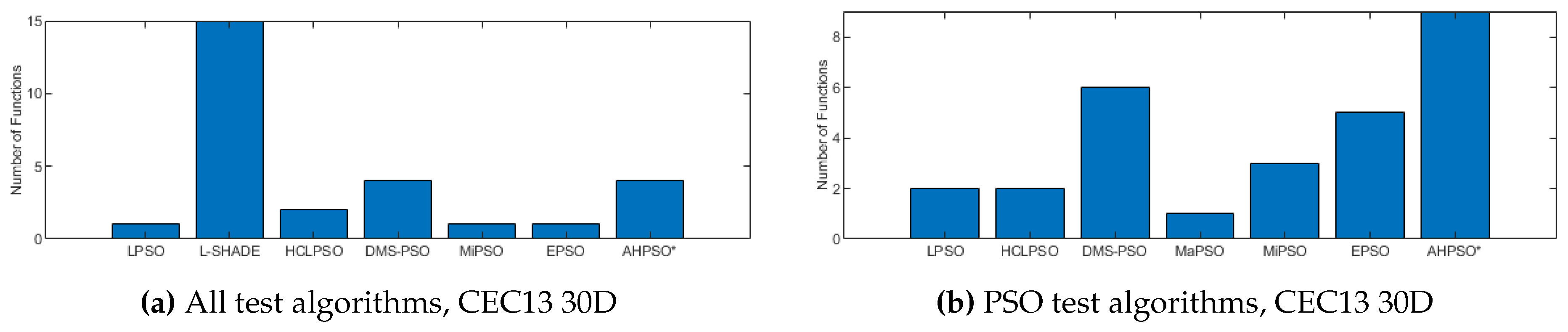
Figure 20.
The total number of best performances achieved by each algorithm with respect to mean error values on the CEC’13 problems at 50-dimensions.
Figure 20.
The total number of best performances achieved by each algorithm with respect to mean error values on the CEC’13 problems at 50-dimensions.
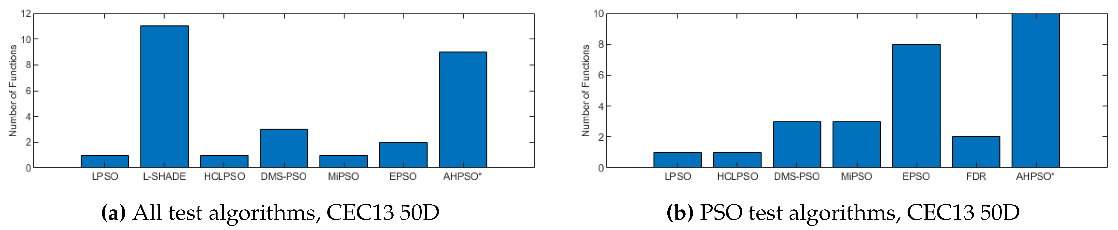
Figure 21.
The total number of best performances achieved by each algorithm with respect to mean error values on the CEC’13 problems at 100-dimensions.
Figure 21.
The total number of best performances achieved by each algorithm with respect to mean error values on the CEC’13 problems at 100-dimensions.
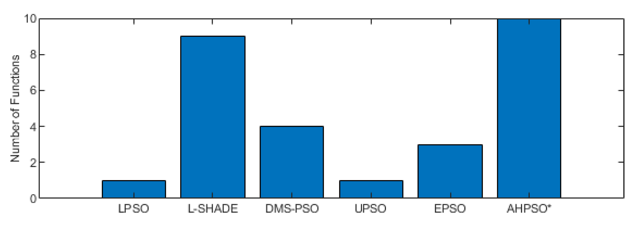
Figure 22.
Wilcoxon Signed Rank Test Results with a Significance Level of for CEC’13 problems at 3 different dimensions.
Figure 22.
Wilcoxon Signed Rank Test Results with a Significance Level of for CEC’13 problems at 3 different dimensions.
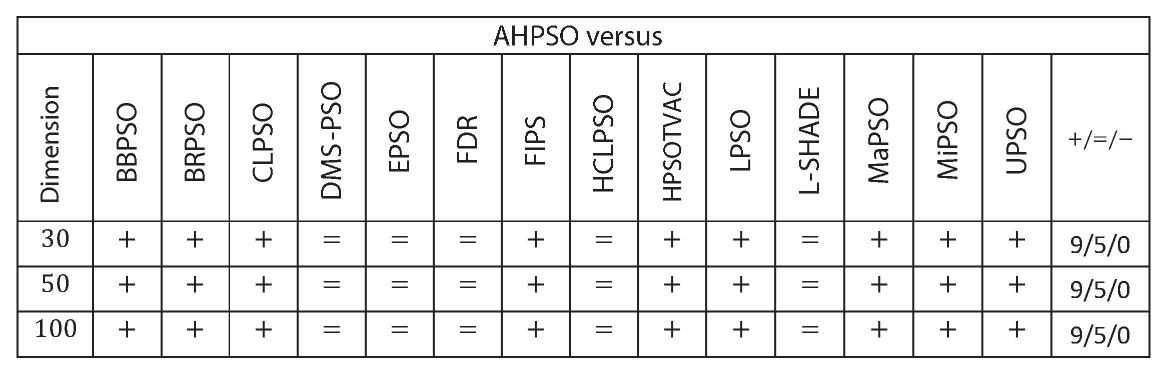
Figure 23.
The total number of best performances achieved by each algorithm with respect to mean error values on the CEC’14 problems at 30-dimensions. Algorithms that did not find any best results on any test functions are not shown.
Figure 23.
The total number of best performances achieved by each algorithm with respect to mean error values on the CEC’14 problems at 30-dimensions. Algorithms that did not find any best results on any test functions are not shown.
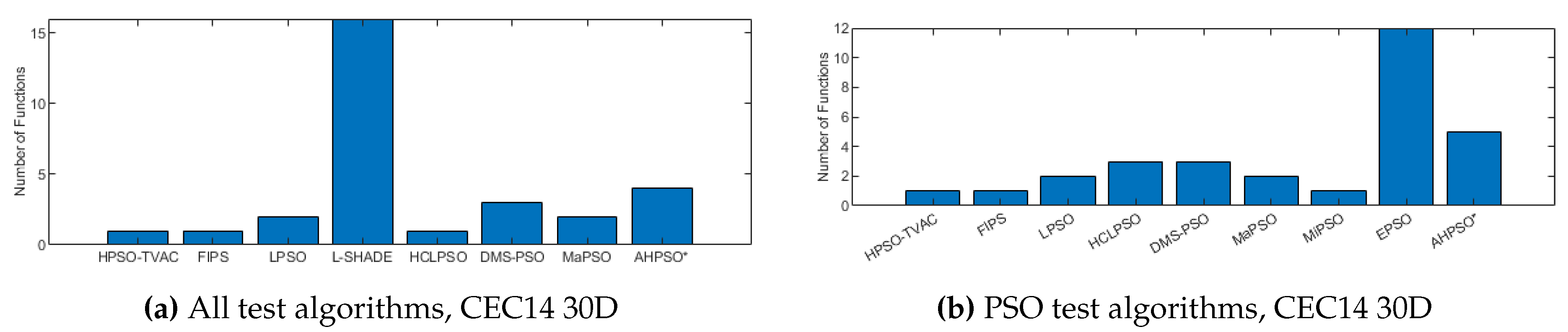
Figure 22 summarises a detailed statistical analysis of the results using the same methodology as detailed earlier for BEPSO. The figure shows us that AHPSO’s performance on the CEC’13 test suite is significantly better than 9 of the 14 comparator algorithms across all dimensions, with no significant difference for the other 5. None of the comparator algorithms were statistically significantly better than AHPSO at any of the dimension. AHPSO performed particularly well on the composition test functions.
Figure 24.
The total number of best performances achieved by each algorithm with respect to mean error values on the CEC’14 problems at 50 and 100 dimensions.
Figure 24.
The total number of best performances achieved by each algorithm with respect to mean error values on the CEC’14 problems at 50 and 100 dimensions.

Figure 25.
Wilcoxon Signed Rank Test Results with a Significance Level of for CEC’14 problems.
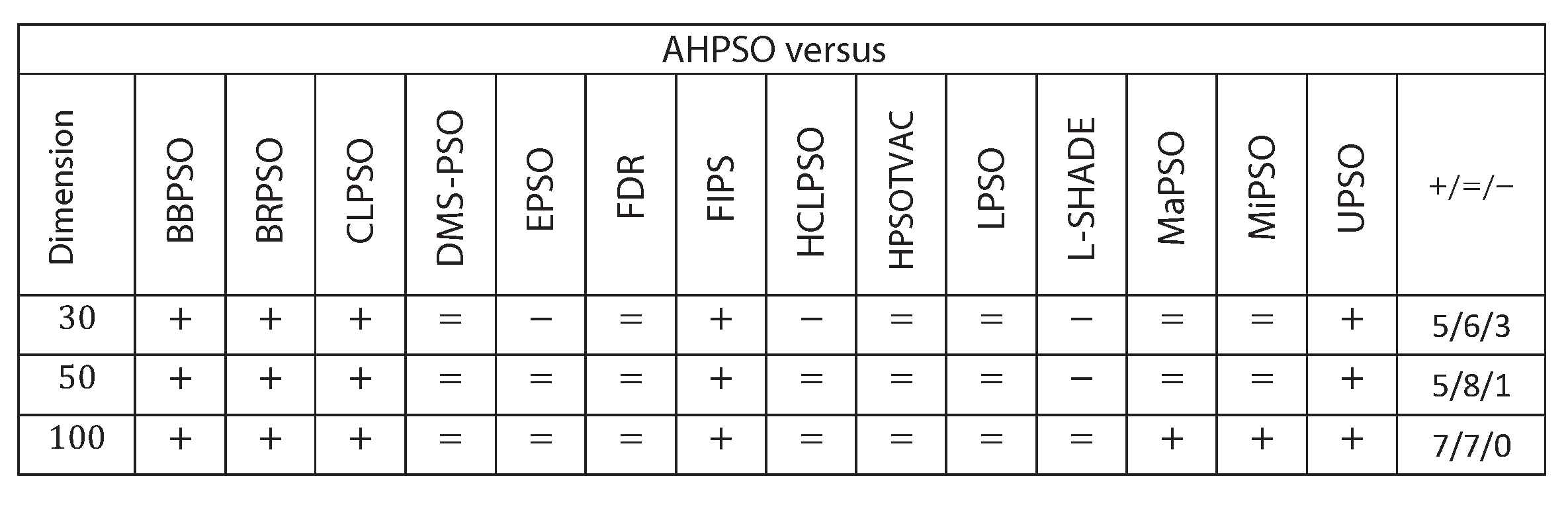
Figure 23, Figure 24 and Figure 25 give the results for AHPSO on the CEC’14 test suite. Relative performance is strong, but not as good as for CEC’13. But we see that the increase in performance with dimension is more marked, with no comparator algorithm statistically better than AHPSO at 100D, and only L-SHADE better at 50D, while, in addition to L-SHADE, two other PSO algorithms (HCLPSO and EPSO) are better at 30D. AHPSO was superior to all other algorithms on the composition test functions.
Figure 26.
The total number of best performances achieved by each algorithm with respect to mean error values on the CEC’17 problems at 30-dimensions. Algorithms that did not find any best results on any test functions are not shown.
Figure 26.
The total number of best performances achieved by each algorithm with respect to mean error values on the CEC’17 problems at 30-dimensions. Algorithms that did not find any best results on any test functions are not shown.
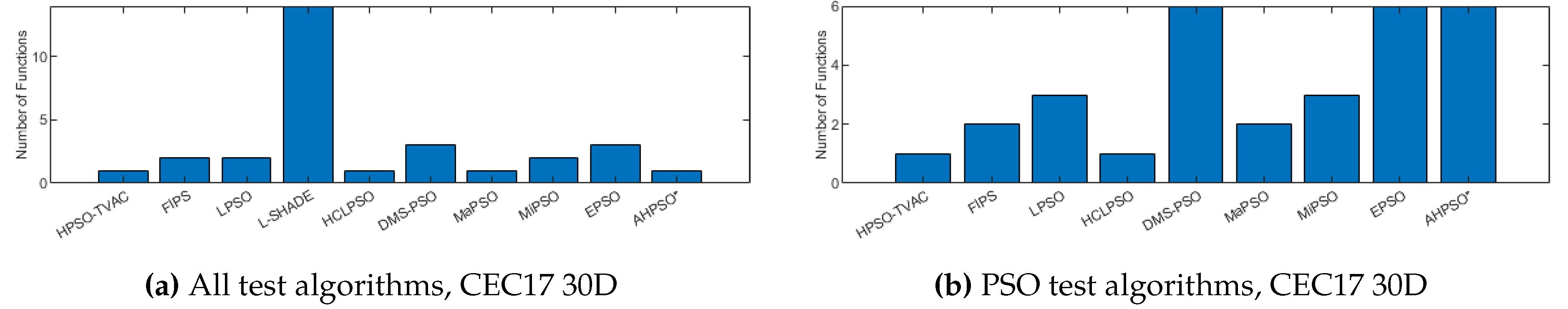
Figure 27.
The total number of best performances achieved by each algorithm with respect to mean error values on the CEC’17 problems at 50 and 100 dimensions.
Figure 27.
The total number of best performances achieved by each algorithm with respect to mean error values on the CEC’17 problems at 50 and 100 dimensions.
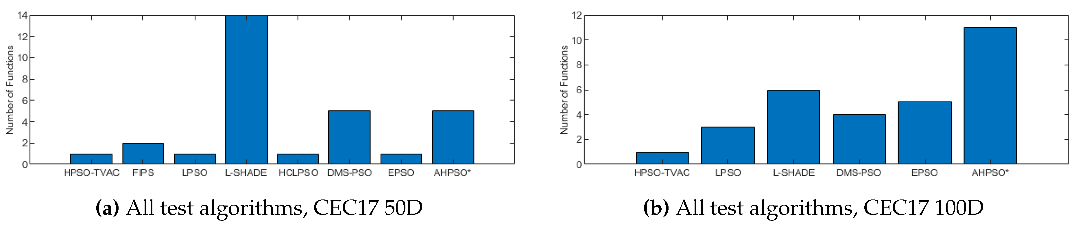
Figure 28.
Wilcoxon Signed Rank Test Results with a Significance Level of for CEC’17 problems.
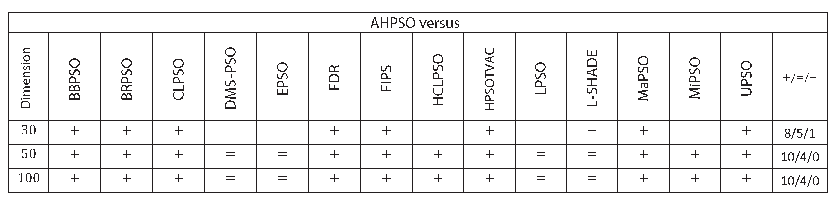
Figure 26, Figure 27 and Figure 28 give the results for the CEC’17 test suite. Again AHPSO’s relative performance is very strong, being statistically significantly better than 10 of the comparator algorithms at the higher dimensions (50D and 100D), while no other algorithms are statistically better than AHPSO at these dimensions. At 30D only L-SHADE is statistically significantly better. AHPSO performed particularly well on multi-modal and composition test functions. At 100D AHPSO exhibited the best performance on more functions (10 out of 29) than all other comparison algorithms (including L-SHADE).
4.4. AHPSO: convergence
Like BEPSO, AHPSO was one of the consistently best performing algorithms across all the test suites. Figure 29, Figure 30 and Figure 31 shows its convergence rates relative to the other top performing algorithms. AHPSO’s converge rates are very similar to the best rates achieved on all the test suites. They are consistently better than those achieved by EPSO and HCLPSO.
5. Constrained Optimisation Problems
Besides verifying the performance of the two novel algorithm on the CEC’13, CEC’14 and CEC’17 benchmark test suites, we examined the performance of BEPSO and AHPSO on 14 constrained real-world problems [50] comprised of process synthesis and design, mechanical engineering and power system problems, comparing against with the same 13 PSO variants and L-SHADE employed in the previous experiments. The complete list of constrained real-world problems are displayed in Table 2. Each problem was tested 30 times, and the maximum number of function evaluations for each problem, , was determined using the following criteria:
where D is the dimension of the problem. The standard penalty method was used to convert the constrained evaluation functions to unconstrained evaluation functions (adding penalties proportional to constraint violations). The same set of general algorithm parameters was used as for the unconstrained test suites.
Figure 32 shows the number of best solutions found by the algorithms across all constrained problems. By this measure AHPSO and L-Shade perform best. AHPSO performed particularly well on the difficult power electronic problems (solving optimal pulse width modulation problems with relatively large numbers of variables and constraints), finding the best known solution for 3 of the 4 problems in this class, with L-SHADE the only other algorithm able to find a (single) best solution in this class. However, on a detailed statistical analysis across all runs on all problems of all algorithms, the best mean rank (2.36) was achieved by BEPSO, the second best (2.5) by L-SHADE, and the third best (2.57) by AHPSO.
Hence, on the constrained real-world problems the two new algorithms, BEPSO and AHPSO, performed extremely strongly in comparison with all other comparator algorithms.
6. Discussion
It is clear from the results presented in the previous sections that the two new novel bio-inspired search algorithms, BEPSO and AHPSO, performed very well across a wide range of unconstrained and constrained optimisation problems, using a single set of parameters for all. They both outperformed most comparator PSO algorithms on most problems. This is more evidence that bio-inspiration – in this case various kinds of animal group behaviours – continues to be a very fruitful source for algorithm design.
The comparative experiments for the two algorithms discussed in the previous section were run independently. Perhaps unsurprisingly, given the nature of these results, a third set of independent runs across the CEC’13, CEC’14 and CEC’17 test suites revealed that there was no statistically significant difference in performance of BEPSO and AHPSO at 30-dimensions, 50-dimensions and 100-dimensions [33].
Both algorithms consistently performed particulary well on the higher dimensional, more complex problems, including unconstrained multi-modal and composition problems, and problems involving many constraints, matching or bettering the performance of all other comparator algorithms. But while their performance on simpler, lower dimension problems was perfectly adequate, it did not match that of the best of the comparator algorithm. This limitations seems to be associated with the deliberately high agent-level heterogeneity that is inherent to the design of BEPSO and AHPSO. This property significantly aids the algorithms in high-dimensional and complex search spaces, while being less effective in low dimensional spaces.
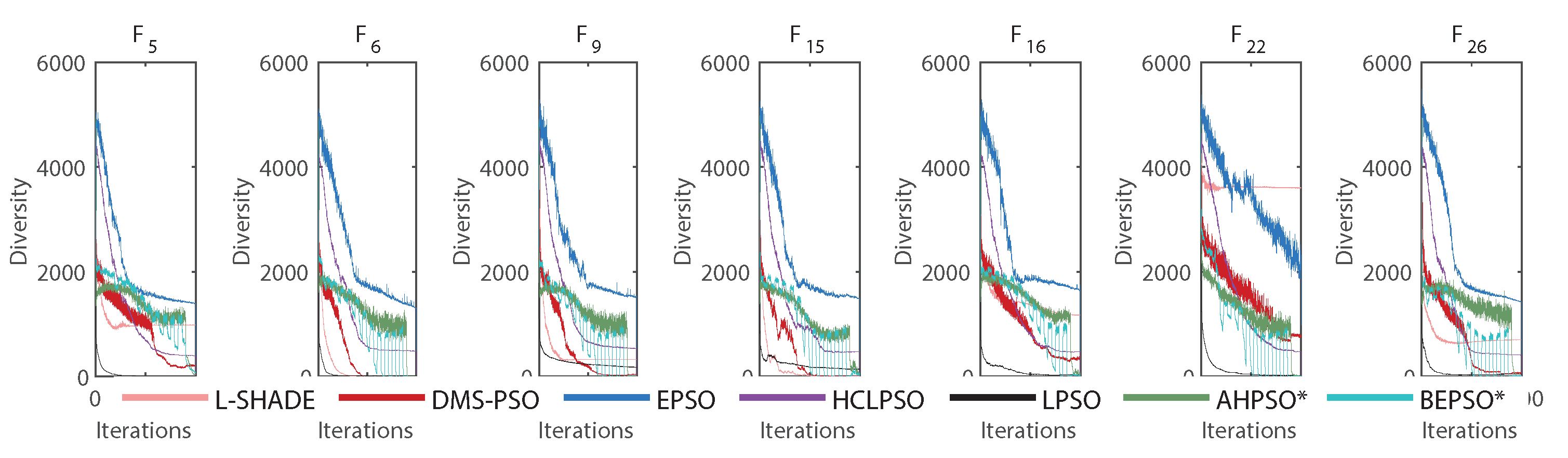
The various mechanisms embedded in both algorithms were partly designed to maintain diversity while enabling efficient search. Figure 33 shows that both BEPSO and AHPSO achieve maintenance of diversity. The graphs use the diversity quantification method proposed in [51]:
where n is the population size, D is the problem dimension and is the average value of , the dth component of the solution vector.
The figure reveals that while EPSO consistently exhibited a more diverse population compared to the other high performing algorithms on the 100-dimensional CEC’17 problems, BEPSO and AHPSO maintained better population diversity compared to all the rest: L-SHADE, LPSO, DMS-PSO and HCLPSO. The trend was repeated across the other test suites for the majority of functions.
Figure 33.
Diversity comparison for best performing algorithms for various representative 100-dimensional CEC’17 problems.
Figure 33.
Diversity comparison for best performing algorithms for various representative 100-dimensional CEC’17 problems.
While the multiple components of the new algorithms, BEPSO and AHPSO, tend to complement each other and in combination maintain diversity, balance exploration and exploitation and enable efficient high-quality search, they do increase the overall complexity of the algorithm. But it is worth noting that many recent variants of metaheuristics, such as [52,53], and several of the comparator algorithms used in the current study, have a much more complex structure than their canonical versions. These variants are discernibly more efficient and are able to handle more diverse problems. Hence the algorithms proposed in this paper are not unusual in comprising a more complex structure and set of interaction mechanisms in comparison to canonical algorithms. However, their individual elements are all simple. Indeed, the slightly more complex framework of the proposed algorithms is inspired by the observation that biological degeneracy plays a vital role in boosting evolvability in nature, and therefore can improve the efficiency of search processes [54]. Biological degeneracy – whereby multiple interacting mechanisms enable multiple different ways of producing an outcome – is an ubiquitous property of biological systems at all levels of organisation [55]. [56] reveals that systems with simple redundancy have considerably lower evolvability than degenerate (e.g., highly versatile) systems with selectable changes of behaviour which enable compensatory actions to occur within the system (exactly what happens at the core of the new algorithms presented in this paper).
However, this increased algorithmic complexity does not necessarily equate to significantly increased computational cost relative to other high performing algorithms. Figure 34 shows the time complexity of BEPSO, AHPSO and the comparator algorithms at various problem dimensions.
The metric proposed in [35] was used to calculate computational complexity for each algorithm using the following steps (originally designed for the CEC13 suite) for each dimension required:
- Step 1 – Calculate the given code (according to the methodology in [35]) and record the computation time as .
- Step 2 – Calculate the computation time just for (CEC13 test suite) for function evaluations on dimension D, record as .
- Step 3 – Calculate the complete computation time for with function evaluations on the same dimension as .
- Step 4 – Repeat step 3 5 times and attain 5 individual values, .
Finally, the time complexity is calculated as .
Figure 34.
Time complexity of BEPSO, AHPSO and comparator algorithms for four dimension sizes.
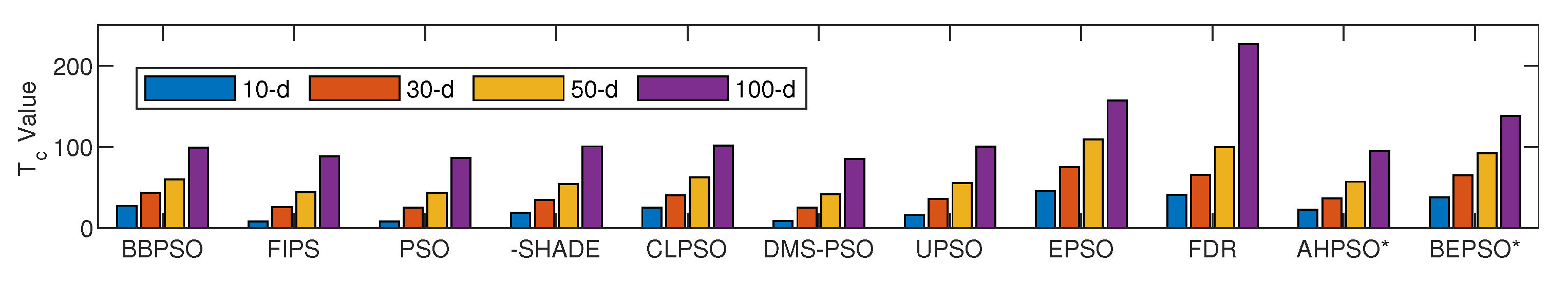
As expected, the basic cannonical PSO obtained the lowest values across all dimensions (although or course it is the worst performing algorithm in terms of solution quality). However, the complexity of the high performing algorithms AHPSO, L-SHADE and HCLPSO across all four dimensions are very similar and not much higher than basic PSO. BEPSO’s complexity is a little higher but still very competitve. In summary, BEPSO and AHPSO exhibit similar, and in some cases, better complexities compared to their peers; however, it is worth highlighting that they exhibit a significantly lower increase in complexity with problem dimensionality (especially AHPSO).
Although cannonical PSO is a very efficient algorithm for many small-scale optimisation problems, as with many metaheuristics, it suffers from the curse of dimensionality. Although the performance of the new PSO algorithms presented in this paper were much less impacted by problem dimensionality compared with other algorithms used in the experiments, various other limitations were identified for possible future improvements. It is clear that the heterogeneous nature of BEPSO and AHPSO provides various strong advantages for the general process of optimisation. However, it is this very property, which makes them so good at complex (multimodal, composition etc) higher dimensional problems, that means that their performance on (simpler) unimodal problems, while perfectly adequate, is consistently worse than some of their competitors, as their speed to solutions is slower. This could be accepted as a clear example of the No Free Lunch Theorem for optimization [57], which tells us that no method can be uniformly excellent over all possible problems, or it could be a prompt to try and improve the algorithms with suitable mechanisms to address this particular issue without destroying their power on other problem types. In general unimodal problems do not require such a careful balance between exploration and exploitation; typically, intensive exploitation is expected to dominate the search process. This is a possible area of future research, either attempting to expand the general efficacy of the methods, or, alternatively, to produce variants of the algorithms that are specialized to specific problem classes.
Considering the efficacy of the new algorithms on high dimensional problems, further investigation on very large-scale problem would be another interesting direction for future work. AHPSO’s superior performance on constrained power electronic problems, and the fact that other researchers have recently successfully used it find the optimal design parameters for hybrid active power filters [58], suggest an expanded investigation of its applications to other problems in the power electronics domain might be very fruitful.
Author Contributions
Conceptualization, F.V.; methodology, F.V. and P.H.; software, F.V.; experiments and data collection, F.V.; formal analysis, F.V.; data curation, F.V.; writing—original draft preparation, F.V. and P.H.; writing—review and editing, F.V. and P.H.; visualization, F.V.; supervision, P.H.; project administration, P.H. All authors have read and agreed to the published version of the manuscript.
Funding
This research received no external funding.
Data Availability Statement
Code for AHPSO and BEPSO algorithms can be found at: https://github.com/FTVarna ; full results data and can be found at: https://doi.org/10.25377/sussex.26146594
Acknowledgments
Thanks to members of the AI group at Sussex, including Chris Buckley and Andy Philippides, for useful discussions on this work.
Conflicts of Interest
The authors declare no conflicts of interest.
References
- Pham, Q.V.; Nguyen, D.C.; Mirjalili, S.; Hoang, D.T.; Nguyen, D.N.; Pathirana, P.N.; Hwang, W.J. Swarm intelligence for next-generation networks: Recent advances and applications. Journal of Network and Computer Applications 2021, 191, 103141. [CrossRef]
- Camci, E.; Kripalani, D.R.; Ma, L.; Kayacan, E.; Khanesar, M.A. An aerial robot for rice farm quality inspection with type-2 fuzzy neural networks tuned by particle swarm optimization-sliding mode control hybrid algorithm. Swarm and Evolutionary Computation 2018, 41, 1–8. [CrossRef]
- Ehteram, M.; Binti Othman, F.; Mundher Yaseen, Z.; Abdulmohsin Afan, H.; Falah Allawi, M.; Bt. Abdul Malek, M.; Najah Ahmed, A.; Shahid, S.; P. Singh, V.; El-Shafie, A. Improving the Muskingum Flood Routing Method Using a Hybrid of Particle Swarm Optimization and Bat Algorithm. Water 2018, 10, 807. [CrossRef]
- Cao, Y.; Ye, Y.; Zhao, H.; Jiang, Y.; Wang, H.; Shang, Y.; Wang, J. Remote sensing of water quality based on HJ-1A HSI imagery with modified discrete binary particle swarm optimization-partial least squares (MDBPSO-PLS) in inland waters: A case in Weishan Lake. Ecological Informatics 2018, 44, 21–32. [CrossRef]
- Thanga Ramya, S.; Arunagiri, B.; Rangarajan, P. Novel effective X-path particle swarm optimization based deprived video data retrieval for smart city. Cluster Computing 2019, 22, 13085–13094. [CrossRef]
- Kennedy, J.; Eberhart, R. Particle swarm optimization. Proceedings of ICNN’95 - International Conference on Neural Networks. IEEE, Vol. 4, pp. 1942–1948. [CrossRef]
- Engelbrecht, A. Particle swarm optimization: Velocity initialization. 2012 IEEE Congress on Evolutionary Computation. IEEE, 2012, pp. 1–8. [CrossRef]
- Engelbrecht, A.P.; Bosman, P.; Malan, K.M. The influence of fitness landscape characteristics on particle swarm optimisers. Natural Computing 2022, 21, 335–345. [CrossRef]
- Jiang, M.; Luo, Y.; Yang, S. Stochastic convergence analysis and parameter selection of the standard particle swarm optimization algorithm. Information Processing Letters 2007, 102, 8–16. [CrossRef]
- Trelea, I.C. The particle swarm optimization algorithm: convergence analysis and parameter selection. Information Processing Letters 2003, 85, 317–325. [CrossRef]
- Varna, F.T.; Husbands, P. HIDMS-PSO: A New Heterogeneous Improved Dynamic Multi-Swarm PSO Algorithm. 2020 IEEE Symposium Series on Computational Intelligence (SSCI). IEEE, 2020, pp. 473–480. [CrossRef]
- Varna, F.T.; Husbands, P. HIDMS-PSO with Bio-inspired Fission-Fusion Behaviour and a Quorum Decision Mechanism. 2021 IEEE Congress on Evolutionary Computation (CEC). IEEE, 2021, pp. 1398–1405. [CrossRef]
- Varna, F.T.; Husbands, P. Genetic Algorithm Assisted HIDMS-PSO: A New Hybrid Algorithm for Global Optimisation. 2021 IEEE Congress on Evolutionary Computation (CEC). IEEE, 2021, pp. 1304–1311. [CrossRef]
- Wang, S.; Liu, G.; Gao, M.; Cao, S.; Guo, A.; Wang, J. Heterogeneous comprehensive learning and dynamic multi-swarm particle swarm optimizer with two mutation operators. Information Sciences 2020, 540, 175–201. [CrossRef]
- Yu, G.R.; Chang, Y.D.; Lee, W.S. Maximum Power Point Tracking of Photovoltaic Generation System Using Improved Quantum-Behavior Particle Swarm Optimization. Biomimetics 2024, 9. [CrossRef]
- Yue, Y.; Cao, L.; Chen, H.; Chen, Y.; Su, Z. Towards an Optimal KELM Using the PSO-BOA Optimization Strategy with Applications in Data Classification. Biomimetics 2023, 8. [CrossRef]
- Shankar, T.; Shanmugavel, S.; Rajesh, A. Hybrid HSA and PSO algorithm for energy efficient cluster head selection in wireless sensor networks. Swarm and Evolutionary Computation 2016, 30, 1–10. [CrossRef]
- Sahoo, B.M.; Pandey, H.M.; Amgoth, T. GAPSO-H: A hybrid approach towards optimizing the cluster based routing in wireless sensor network. Swarm and Evolutionary Computation 2021, 60, 100772. [CrossRef]
- Liang, J.; Qin, A.; Suganthan, P.; Baskar, S. Comprehensive learning particle swarm optimizer for global optimization of multimodal functions. IEEE Transactions on Evolutionary Computation 2006, 10, 281–295. [CrossRef]
- Lynn, N.; Suganthan, P.N. Heterogeneous comprehensive learning particle swarm optimization with enhanced exploration and exploitation. Swarm and Evolutionary Computation 2015, 24, 11–24. [CrossRef]
- Changhe Li.; Shengxiang Yang.; Trung Thanh Nguyen. A Self-Learning Particle Swarm Optimizer for Global Optimization Problems. IEEE Transactions on Systems, Man, and Cybernetics, Part B (Cybernetics) 2012, 42, 627–646. [CrossRef]
- Kennedy, J. Small worlds and mega-minds: effects of neighborhood topology on particle swarm performance. Proceedings of the 1999 Congress on Evolutionary Computation-CEC99 (Cat. No. 99TH8406). IEEE, 1999, pp. 1931–1938. [CrossRef]
- Kennedy, J.; Mendes, R. Population structure and particle swarm performance. Proceedings of the 2002 Congress on Evolutionary Computation, CEC 2002. IEEE, 2002, Vol. 2, pp. 1671–1676. [CrossRef]
- Suganthan, P. Particle swarm optimiser with neighbourhood operator. Proceedings of the 1999 Congress on Evolutionary Computation-CEC99 (Cat. No. 99TH8406). IEEE, pp. 1958–1962. [CrossRef]
- Varna, F.T.; Husbands, P. HIDMS-PSO Algorithm with an Adaptive Topological Structure. 2021 IEEE Symposium Series on Computational Intelligence (SSCI). IEEE, 2021, pp. 1–8. [CrossRef]
- Liang, J.J.; Suganthan, P.N. Dynamic multi-swarm particle swarm optimizer. Proceedings - 2005 IEEE Swarm Intelligence Symposium, SIS 2005. IEEE, 2005, Vol. 2005, pp. 127–132. [CrossRef]
- Trillo, P.A.; Benson, C.S.; Caldwell, M.S.; Lam, T.L.; Pickering, O.H.; Logue, D.M. The Influence of Signaling Conspecific and Heterospecific Neighbors on Eavesdropper Pressure. Frontiers in Ecology and Evolution 2019, 7. [CrossRef]
- Lilly, M.V.; Lucore, E.C.; Tarvin, K.A. Eavesdropping grey squirrels infer safety from bird chatter. PLOS ONE 2019, 14, e0221279. [CrossRef]
- Hamilton, W.D. The genetical evolution of social behaviour. I. Journal of Theoretical Biology 1964, 7, 1–16. [CrossRef]
- Roberts, G. Cooperation: How Vampire Bats Build Reciprocal Relationships. Current Biology 2020, 30, R307–R309. [CrossRef]
- Connor, R.C. Pseudo-reciprocity: Investing in mutualism. Animal Behaviour 1986, 34, 1562–1566. [CrossRef]
- Wickelgren, W.A. Speed-accuracy tradeoff and information processing dynamics. Acta Psychology 1977, 41, 67–85.
- Varna, F.T. Design and Implementation of Bio-inspired Heterogeneous Particle Swarm Optimisation Algorithms for Unconstrained and Constrained Problems. Phd thesis, University of Sussex, 2023.
- Varna, F.T.; Husbands, P. BIS: A New Swarm-Based Optimisation Algorithm. 2020 IEEE Symposium Series on Computational Intelligence (SSCI). IEEE, 2020, pp. 457–464. [CrossRef]
- Liang, J.; Qu, B.; Suganthan, P. Problem Definitions and Evaluation Criteria for the CEC 2013 Special Session on Real-Parameter Optimization, Vol. 34: Technical Report 201212. Technical report, Computational Intelligence Laboratory, Zhengzhou University, Zhengzhou, China and Nanyang Technological University, Singapore, 2013.
- Liang, J.; Qu, B.; Suganthan, P. Problem Definitions and Evaluation Criteria for the CEC 2014 Special Session and Competition on Single Objective Real-Parameter Numerical Optimization. Technical report, Computational Intelligence Laboratory, Zhengzhou University, Zhengzhou China and Technical Report, Nanyang Technological University, Singapore, 2014.
- Awad, N.; Ali, M.; Suganthan, P.; Liang, J.; Qu, B. Problem Definitions and Evaluation Criteria for the CEC 2017 Special Session and Competition on Single Objective Real-Parameter Numerical Optimization. Technical report, School of EEE, Nanyang Technological University, Singapore, School of Computer Information Systems, Jordan University of Science and Technology, Jordan, School of Electrical Engineering, Zhengzhou University, Zhengzhou, China, 2016.
- Yue, N.; Yue, P.; Price, K.; Suganthan, P.; Liang, J.; Ali, M.; Qu, B. Problem Definitions and Evaluation Criteria for the CEC 2020 Special Session and Competition on Single Objective Bound Constrained Numerical Optimization, 2019.
- Tanabe, R.; Fukunaga, A.S. Improving the search performance of SHADE using linear population size reduction. 2014 IEEE Congress on Evolutionary Computation (CEC). IEEE, 2014, pp. 1658–1665. [CrossRef]
- Kennedy, J. Bare bones particle swarms. Proceedings of the 2003 IEEE Swarm Intelligence Symposium. SIS’03 (Cat. No.03EX706). IEEE, pp. 80–87. [CrossRef]
- Settles, M.; Soule, T. Breeding swarms. Proceedings of the 2005 conference on Genetic and evolutionary computation - GECCO ’05; ACM Press: New York, New York, USA, 2005; p. 161. [CrossRef]
- Mendes, R.; Kennedy, J.; Neves, J. The Fully Informed Particle Swarm: Simpler, Maybe Better. IEEE Transactions on Evolutionary Computation 2004, 8, 204–210. [CrossRef]
- Peram, T.; Veeramachaneni, K.; Mohan, C. Fitness-distance-ratio based particle swarm optimization. Proceedings of the 2003 IEEE Swarm Intelligence Symposium. SIS’03 (Cat. No.03EX706). IEEE, pp. 174–181. [CrossRef]
- Parsopoulos, K.; Vrahatis, M. UPSO: A Unified Particle Swarm Optimization Scheme. In International Conference of Computational Methods in Sciences and Engineering 2004 (ICCMSE 2004); CRC Press, 2019; pp. 868–873. [CrossRef]
- Lynn, N.; Suganthan, P.N. Ensemble particle swarm optimizer. Applied Soft Computing 2017, 55, 533–548. [CrossRef]
- Ratnaweera, A.; Halgamuge, S.; Watson, H. Self-Organizing Hierarchical Particle Swarm Optimizer With Time-Varying Acceleration Coefficients. IEEE Transactions on Evolutionary Computation 2004, 8, 240–255. [CrossRef]
- Shi, Y.; Eberhart, R. IEEE International Conference on Evolutionary Computation 1998. IEEE. [CrossRef]
- Hasanzadeh, M.; Meybodi, M.R.; Ebadzadeh, M.M. Adaptive Parameter Selection in Comprehensive Learning Particle Swarm Optimizer; 2014; pp. 267–276. [CrossRef]
- Derrac, J.; Garcia, S.; Molina, D.; Herrera, F. A practical tutorial on the use of nonparametric statistical tests as a methodology for comparing evolutionary and swarm intelligence algorithms. Swarm Evol. Comput. 2011, 1, 3–18. [CrossRef]
- Kumar, A.; Wu, G.; Ali, M.Z.; Mallipeddi, R.; Suganthan, P.N.; Das, S. A test-suite of non-convex constrained optimization problems from the real-world and some baseline results. Swarm and Evolutionary Computation 2020, 56, 100693. [CrossRef]
- A. P. Engelbrecht. Fundamentals of Computational Swarm Intelligence; Wiley, 2005.
- Li, W.; Meng, X.; Huang, Y.; Fu, Z.H. Multipopulation cooperative particle swarm optimization with a mixed mutation strategy. J. Inf. Sci. 2020, 529, 179–196. [CrossRef]
- Wood, D. Hybrid cuckoo search optimization algorithms applied to complex wellbore trajectories aided by dynamic, chaos-enhanced, fat-tailed distribution sampling and metaheuristic profiling. Nat. Gas Sci. Eng. 2016, 34, 236–252. [CrossRef]
- Husbands, P.; Philippides, A.; Vargas, P.; Buckley, C.; Fine, P.; DiPaolo, E.; O’Shea, M. Spatial, temporal, and modulatory factors affecting GasNet evolvability in a visually guided robotics task. Complexity 2010, 16, 35–44. [CrossRef]
- Edelman, G.; Gally, J. Degeneracy and complexity in biological systems. Proc. Natl. Acad. Sci. 2001, 98, 13763––13768. [CrossRef]
- Whitacre, J.; Bender, A. Degeneracy: A design principle for achieving robustness and evolvability. J. Theor. Biol. 2010, 263, 143–153. [CrossRef]
- Wolpert, D.H.; Macready, W.G. No Free Lunch Theorems for Optimization. IEEE Transactions on Evolutionary Computation 1997, 1, 67–82. [CrossRef]
- Chauhan, D.; Yadav, A. Optimizing the parameters of hybrid active power filters through a comprehensive and dynamic multi-swarm gravitational search algorithm. Engineering Applications of Artificial Intelligence 2023, 123, 106469. [CrossRef]
Figure 2.
The accumulator decision model showing the particle’s bias towards the particle at time t
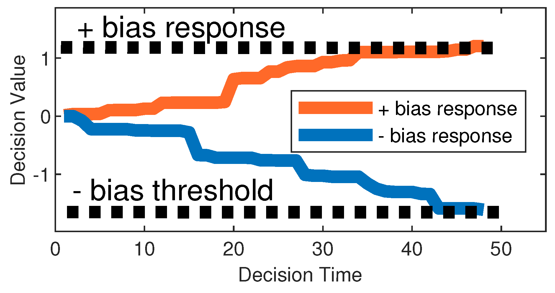
Figure 4.
The BEPSO algorithm
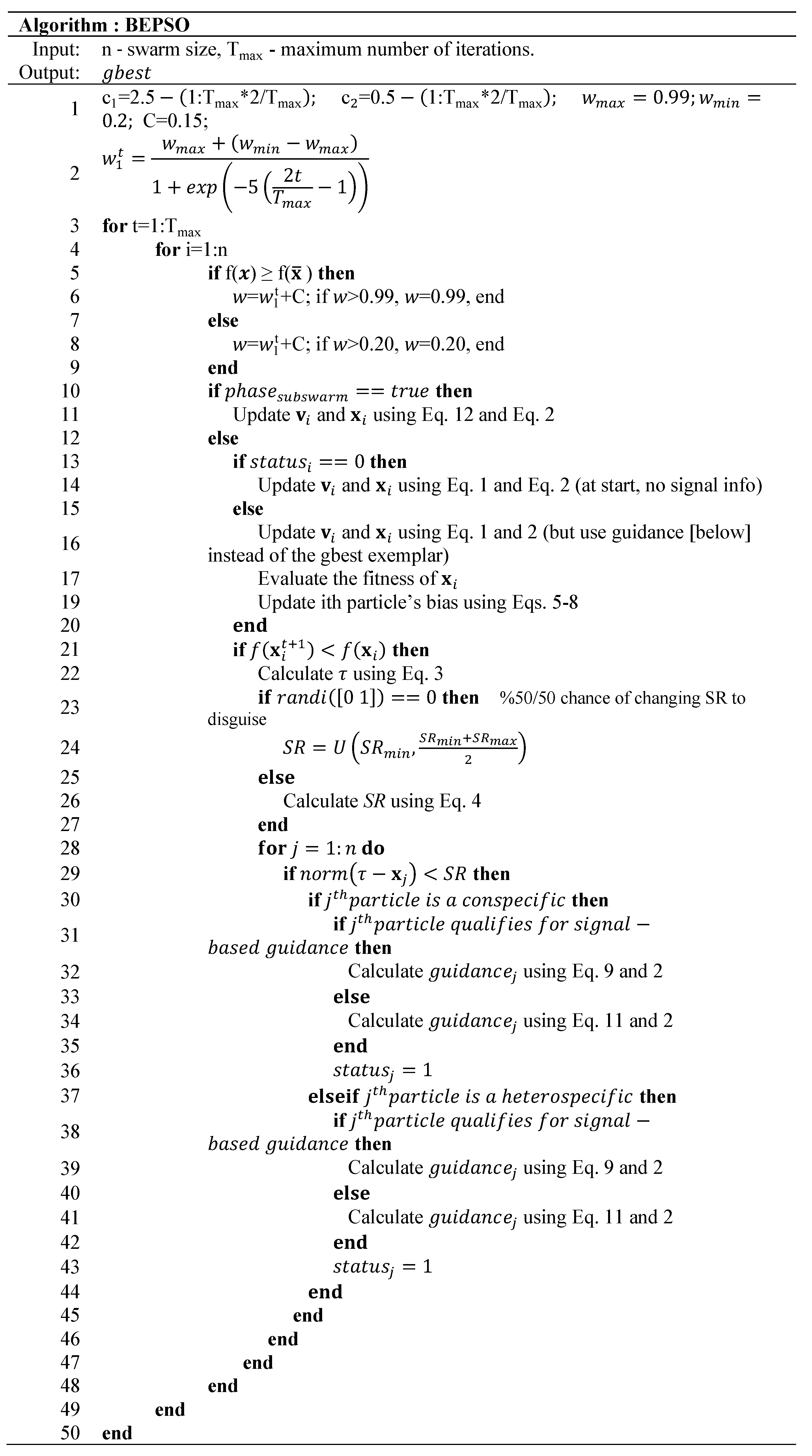
Figure 5.
The AHPSO algorithm
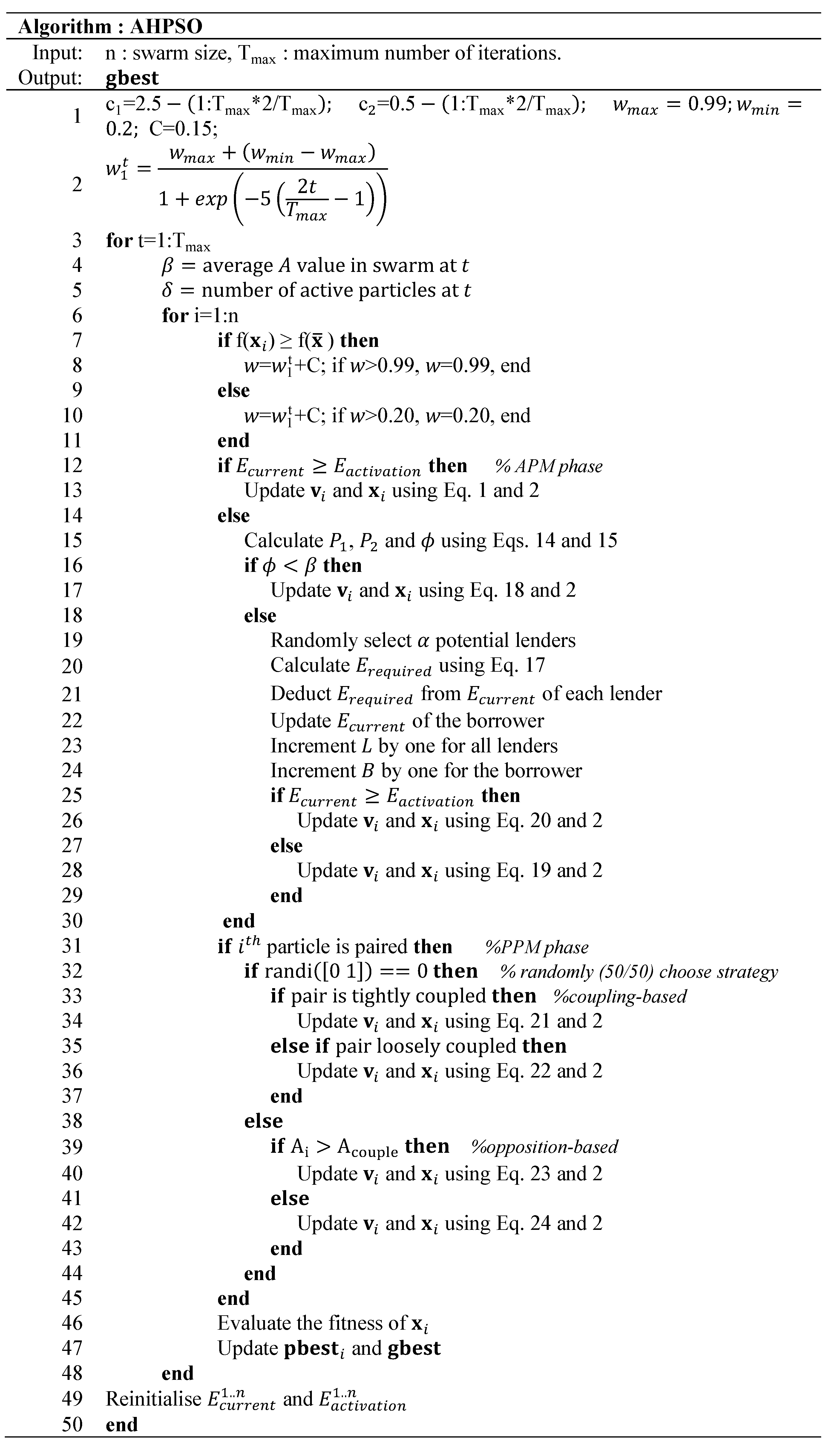
Figure 6.
The total number of best performances achieved by each algorithm with respect to mean error values on the CEC’13 problems at 30-dimensions. Algorithms that did not find any best results on any test functions are not shown.
Figure 6.
The total number of best performances achieved by each algorithm with respect to mean error values on the CEC’13 problems at 30-dimensions. Algorithms that did not find any best results on any test functions are not shown.
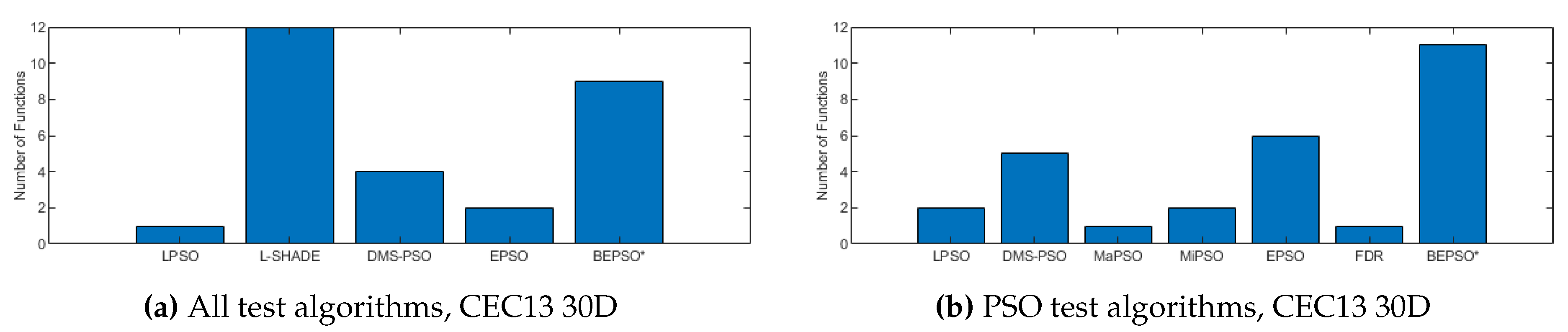
Figure 7.
The total number of best performances achieved by each algorithm with respect to mean error values on the CEC’13 problems at 50-dimensions.
Figure 7.
The total number of best performances achieved by each algorithm with respect to mean error values on the CEC’13 problems at 50-dimensions.
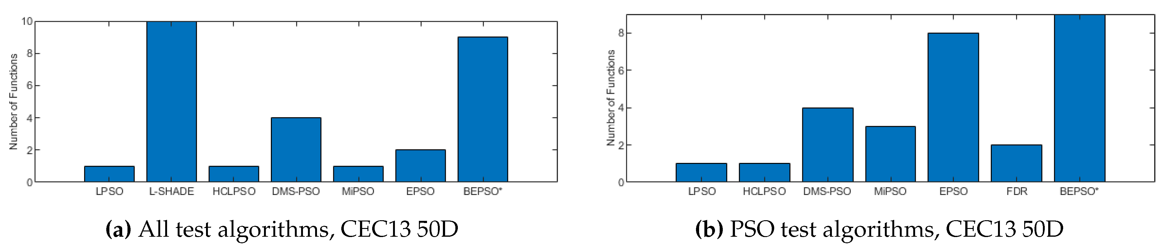
Figure 8.
The total number of best performances achieved by each algorithm with respect to mean error values on the CEC’13 problems at 100-dimensions.
Figure 8.
The total number of best performances achieved by each algorithm with respect to mean error values on the CEC’13 problems at 100-dimensions.
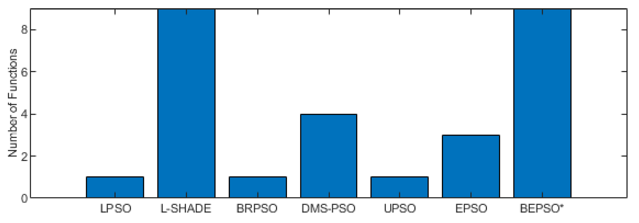
Figure 9.
Wilcoxon Signed Rank Test Results with a Significance Level of for CEC’13 problems at 3 different dimensions.
Figure 9.
Wilcoxon Signed Rank Test Results with a Significance Level of for CEC’13 problems at 3 different dimensions.
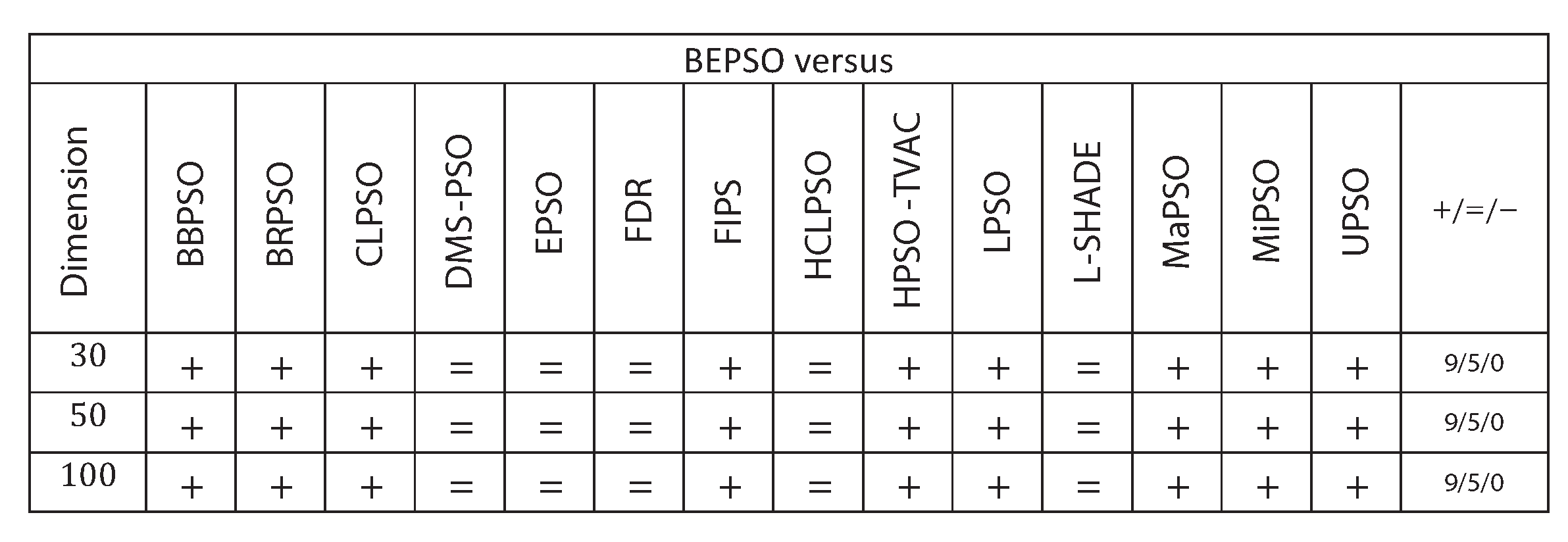
Figure 10.
The total number of best performances achieved by each algorithm with respect to mean error values on the CEC’14 problems at 30-dimensions.
Figure 10.
The total number of best performances achieved by each algorithm with respect to mean error values on the CEC’14 problems at 30-dimensions.
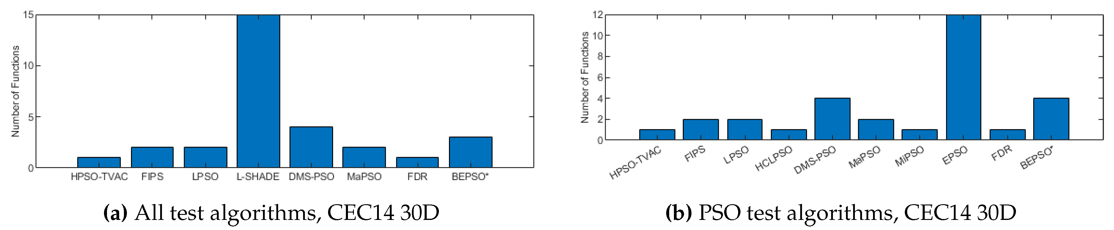
Figure 11.
The total number of best performances achieved by each algorithm with respect to mean error values on the CEC’14 problems at 50 and 100 dimensions.
Figure 11.
The total number of best performances achieved by each algorithm with respect to mean error values on the CEC’14 problems at 50 and 100 dimensions.
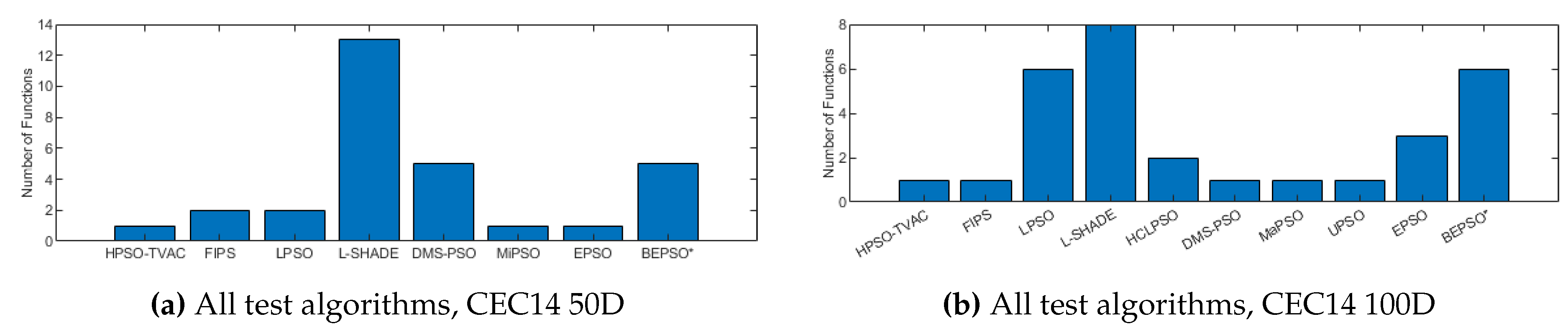
Figure 12.
Wilcoxon Signed Rank Test Results with a Significance Level of for CEC’14 problems.
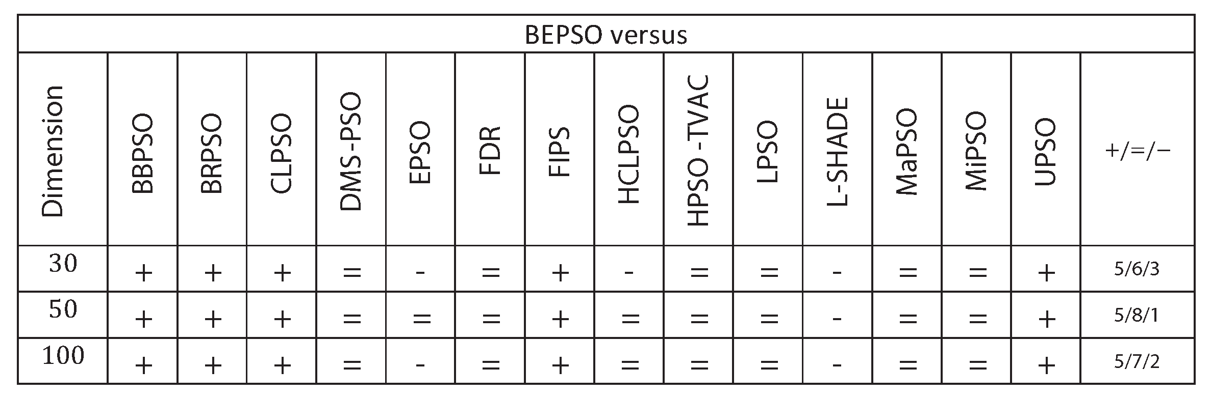
Figure 13.
The total number of best performances achieved by each algorithm with respect to mean error values on the CEC’17 problems at 30-dimensions.
Figure 13.
The total number of best performances achieved by each algorithm with respect to mean error values on the CEC’17 problems at 30-dimensions.
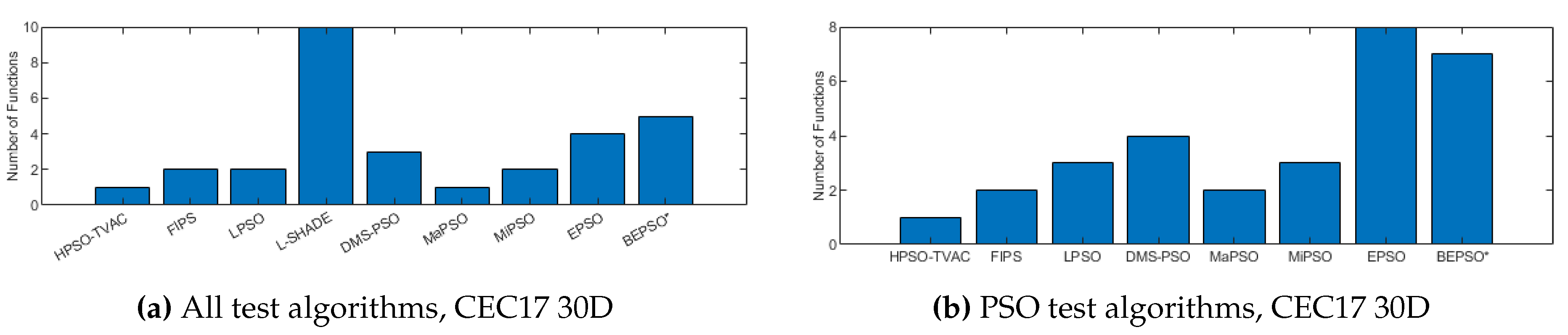
Figure 14.
The total number of best performances achieved by each algorithm with respect to mean error values on the CEC’17 problems at 50 and 100 dimensions.
Figure 14.
The total number of best performances achieved by each algorithm with respect to mean error values on the CEC’17 problems at 50 and 100 dimensions.
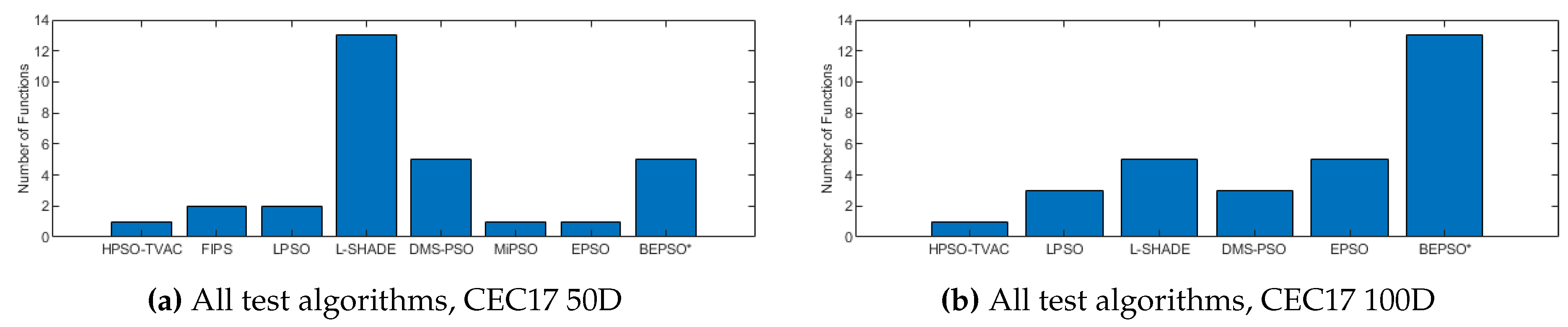
Figure 15.
Wilcoxon Signed Rank Test Results with a Significance Level of for CEC’17 problems.
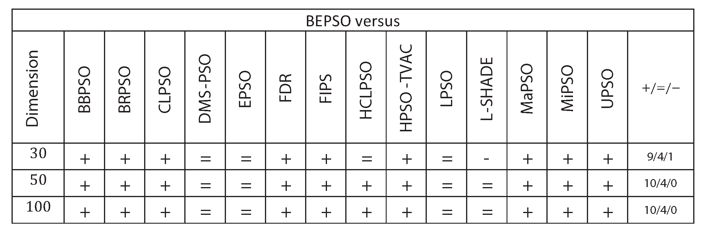
Figure 16.
Average convergence rate comparison of BEPSO with L-SHADE, EPSO, HCLPSO and DMS-PSO on various 100-dimensional CEC’13 problems.
Figure 16.
Average convergence rate comparison of BEPSO with L-SHADE, EPSO, HCLPSO and DMS-PSO on various 100-dimensional CEC’13 problems.
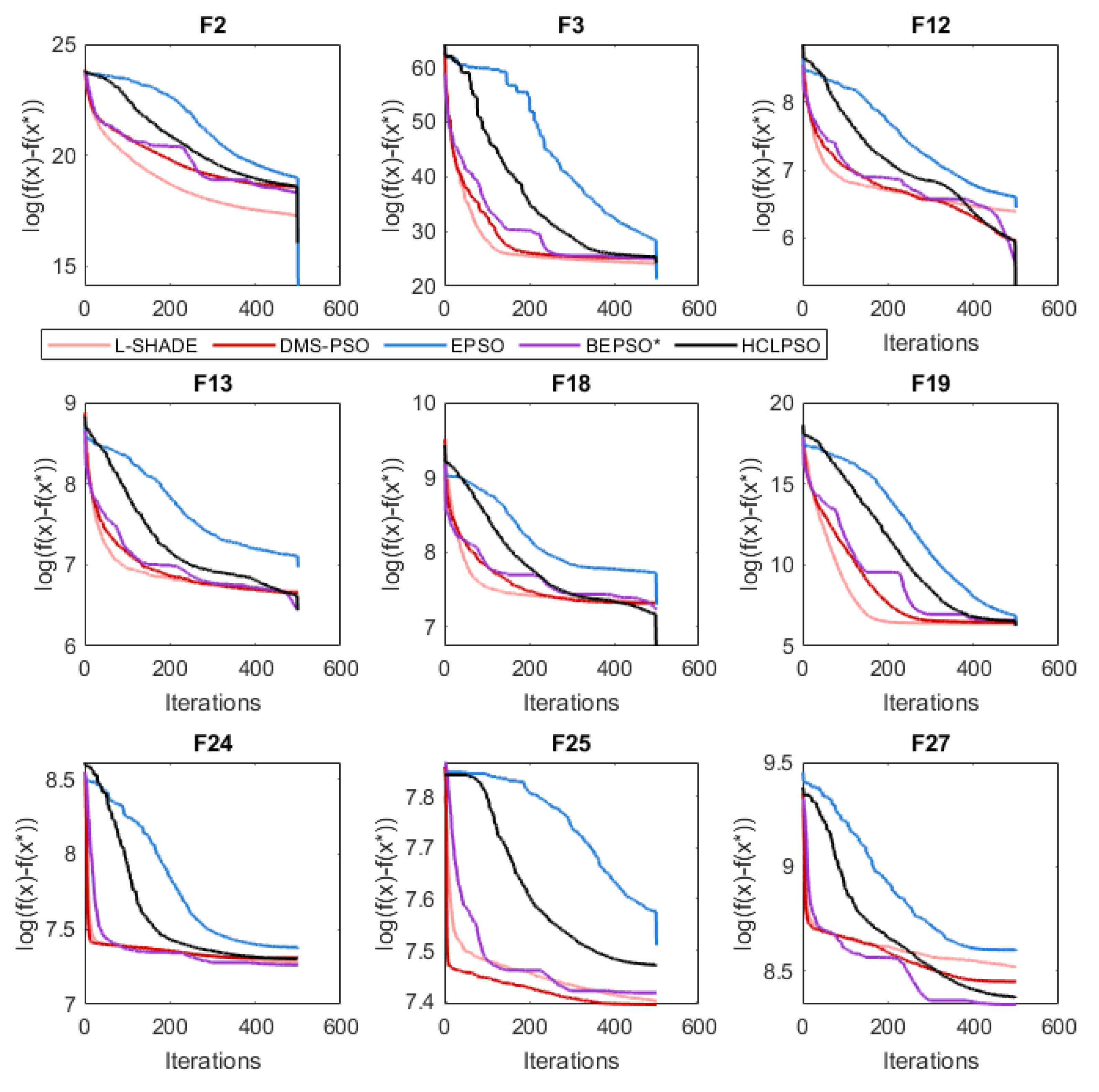
Figure 17.
Average convergence rate comparison of BEPSO with L-SHADE, EPSO, HCLPSO and DMS-PSO on various 100-dimensional CEC’14 problems.
Figure 17.
Average convergence rate comparison of BEPSO with L-SHADE, EPSO, HCLPSO and DMS-PSO on various 100-dimensional CEC’14 problems.
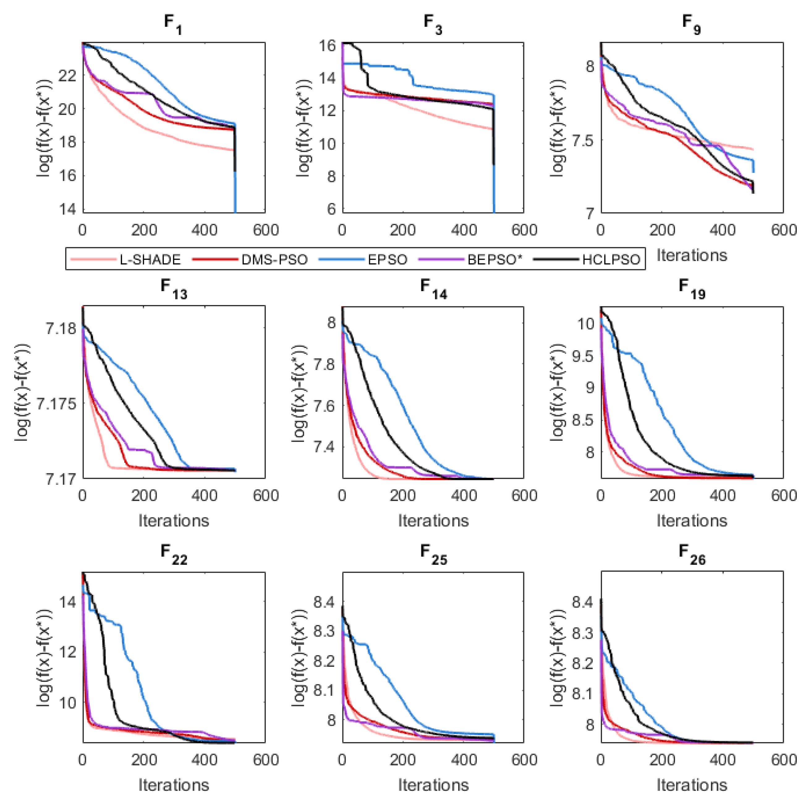
Figure 18.
Average convergence rate comparison of BEPSO with L-SHADE, EPSO, HCLPSO and DMS-PSO on various 100-dimensional CEC’17 problems.
Figure 18.
Average convergence rate comparison of BEPSO with L-SHADE, EPSO, HCLPSO and DMS-PSO on various 100-dimensional CEC’17 problems.
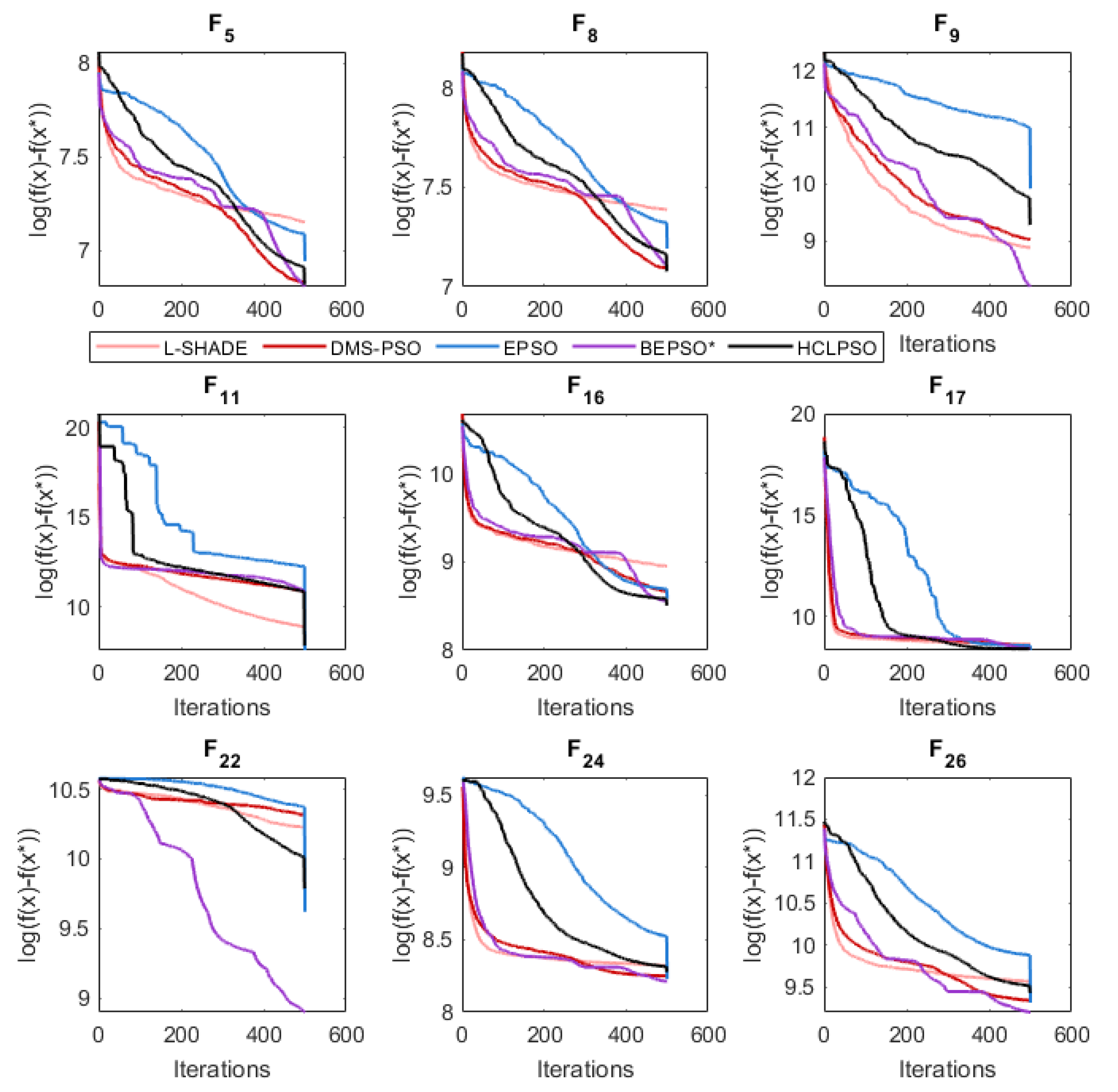
Figure 29.
Average convergence rate comparison of AHPSO with L-SHADE, EPSO, HCLPSO and DMS-PSO on various 100-dimensional CEC’13 problems.
Figure 29.
Average convergence rate comparison of AHPSO with L-SHADE, EPSO, HCLPSO and DMS-PSO on various 100-dimensional CEC’13 problems.
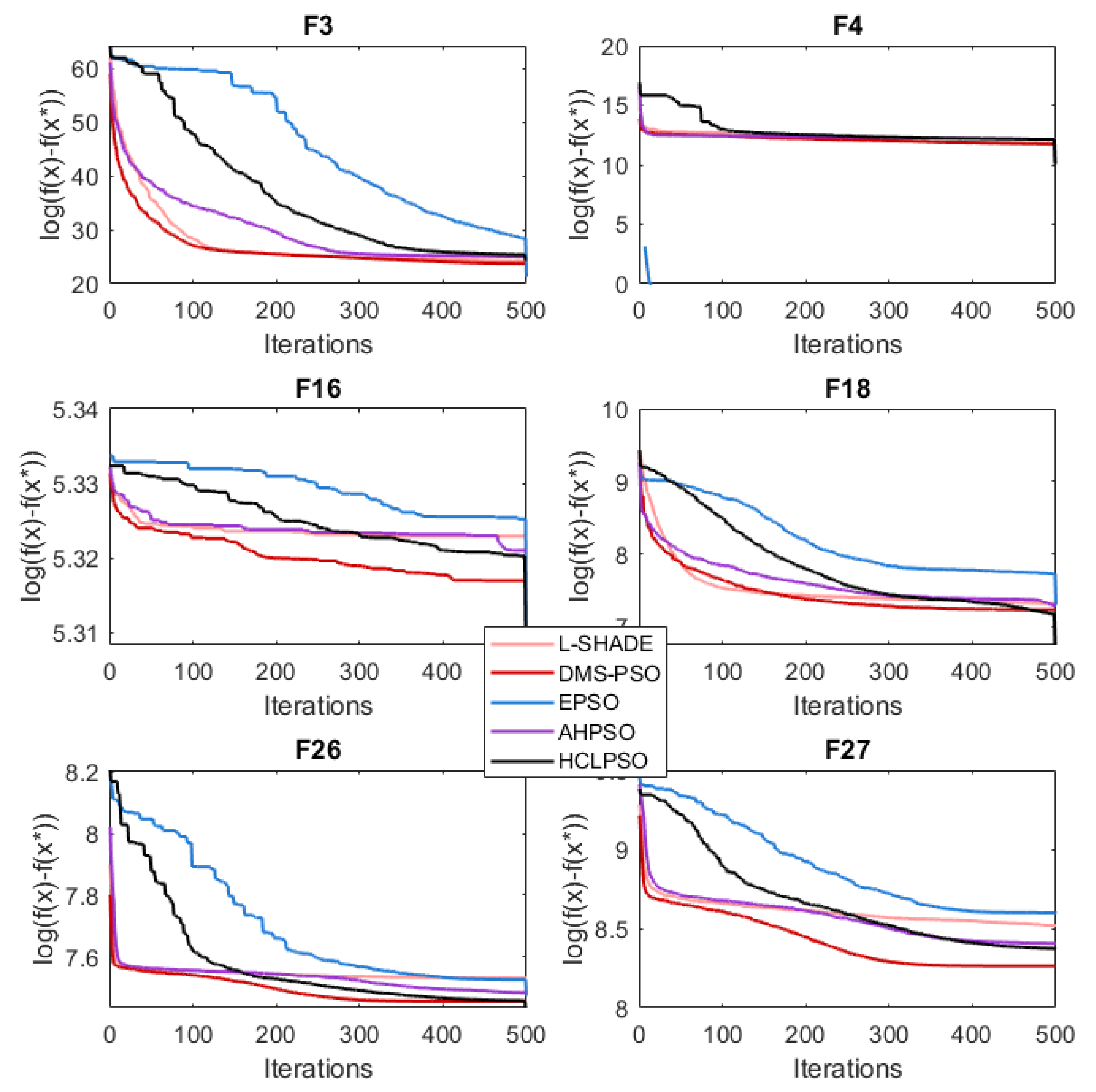
Figure 30.
Average convergence rate comparison of AHPSO with L-SHADE, EPSO, HCLPSO and DMS-PSO on various 100-dimensional CEC’14 problems.
Figure 30.
Average convergence rate comparison of AHPSO with L-SHADE, EPSO, HCLPSO and DMS-PSO on various 100-dimensional CEC’14 problems.
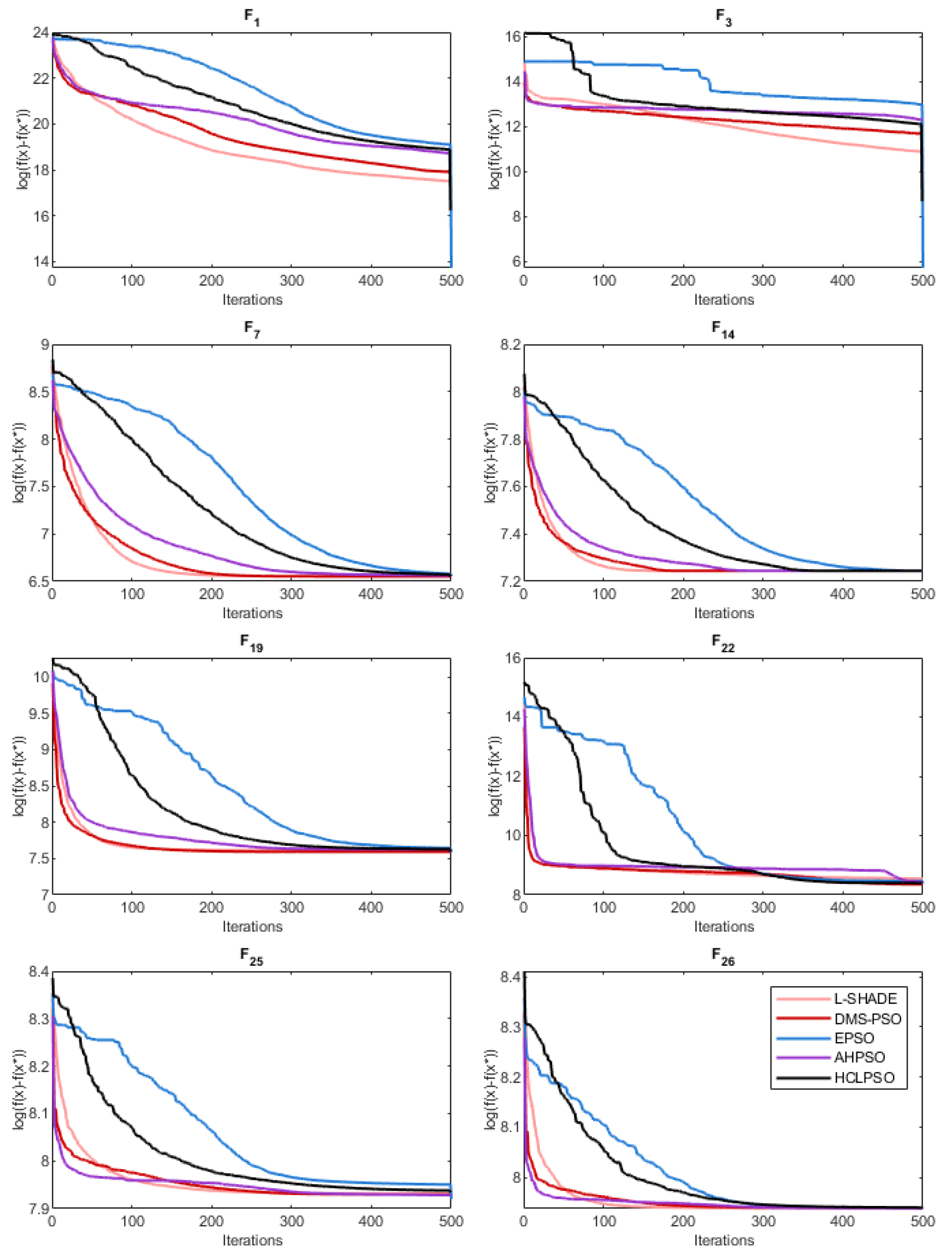
Figure 31.
Average convergence rate comparison of AHPSO with L-SHADE, EPSO, HCLPSO and DMS-PSO on various 100-dimensional CEC’17 problems.
Figure 31.
Average convergence rate comparison of AHPSO with L-SHADE, EPSO, HCLPSO and DMS-PSO on various 100-dimensional CEC’17 problems.
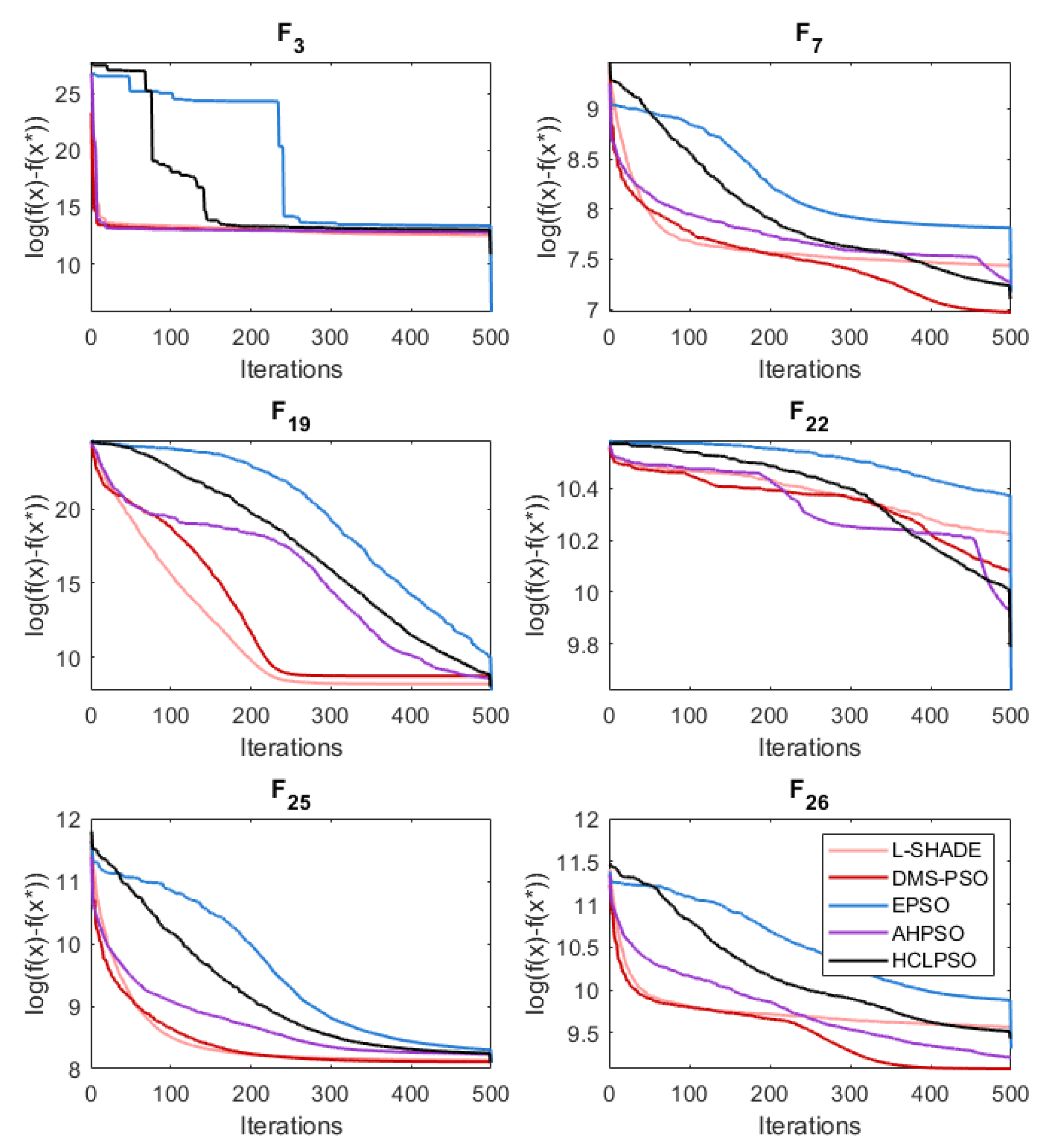
Figure 32.
Total number of constrained real-world problems solved (lowest mean error value obtained) by the proposed and comparator algorithms. * = no best solutions found.
Figure 32.
Total number of constrained real-world problems solved (lowest mean error value obtained) by the proposed and comparator algorithms. * = no best solutions found.
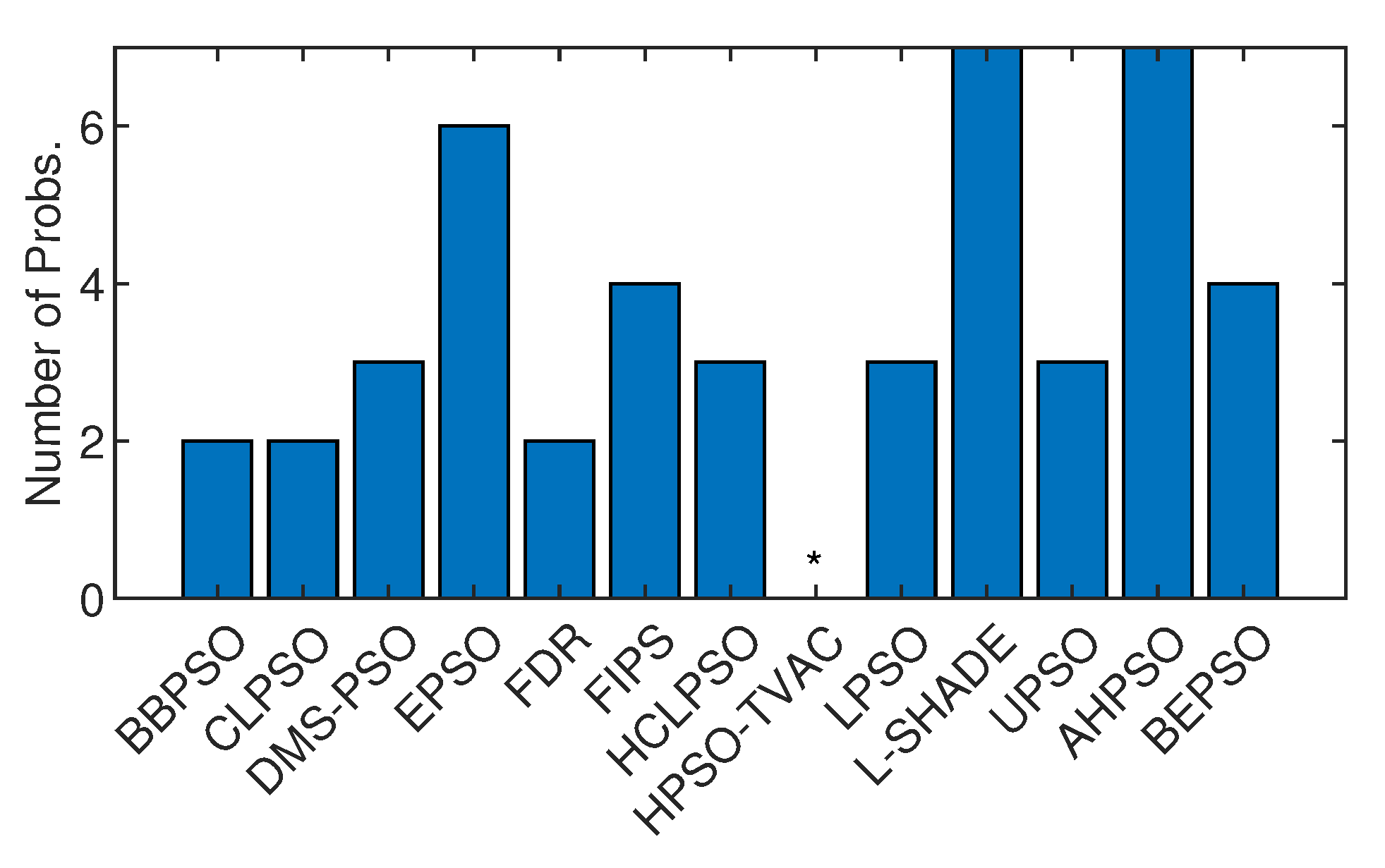

Table 1.
The comparator algorithms used in the detailed investigations of BEPSO and AHPSO, along with their key parameter values.
Table 1.
The comparator algorithms used in the detailed investigations of BEPSO and AHPSO, along with their key parameter values.
| Key | Algorithm | Parameters |
| L-Shade [39] | SHADE with linear population reduction | see [39] |
| BBPSO [40] | Bare bones PSO | see [40] |
| BreedingPSO [41] | A GA/PSO hybrid | w=0.8 - 0.6, |
| HCLPSO [20] | Heterogeneous comprehensive learning PSO | w=0.99–0.29,, |
| CLPSO [19] | Comprehensive learning PSO | w=0.9–0.2; |
| FIPS [42] | Fully informed PSO | |
| FDR-PSO [43] | Fitness distance ratio PSO | w=0.9–0.4, |
| UPSO [44] | Unified PSO | |
| EPSO [45] | Ensemble PSO | see [45] |
| DMS-PSO [26] | Dynamic multi-swarm PSO | |
| HPSO-TVAC [46] | Hierarchical PSO, time-varying coefficients | |
| LPSO [47] | Linearly decreasing inertial weight PSO | |
| maPSO [48] | macroscopic PSO | |
| miPSO [48] | microscopic PSO |
Table 2.
Details of the 14 constrained real-world problems. D is the number of decision variables, g and h are the number of inequality and equality constraints, respectively and is the best known objective function value.
Table 2.
Details of the 14 constrained real-world problems. D is the number of decision variables, g and h are the number of inequality and equality constraints, respectively and is the best known objective function value.
| Problem | D | g | h | ||
| Process Synthesis and Design Problems | |||||
| RC01 | Process flow sheeting problem | 3 | 3 | 0 | 1.0765430833E+00 |
| RC02 | Process synthesis problem | 7 | 9 | 0 | 2.9248305537E+00 |
| Mechanical Engineering Problems | |||||
| RC03 | Weight minimization of a speed reducer | 7 | 11 | 0 | 2.9944244658E+03 |
| RC04 | Pressure vessel design | 4 | 4 | 0 | 5.8853327736E+03 |
| RC05 | Three-bar truss design problem | 2 | 3 | 0 | 2.6389584338E+02 |
| RC06 | Step-cone pulley problem | 5 | 8 | 3 | 1.6069868725E+01 |
| RC07 | 10-bar truss design | 10 | 3 | 0 | 5.2445076066E+02 |
| RC08 | Rolling element bearing | 10 | 9 | 0 | 1.4614135715E+04 |
| RC09 | Gas transmission compressor design | 4 | 1 | 0 | 2.9648954173E+06 |
| RC10 | Gear train design | 4 | 1 | 1 | 0.0000000000E+00 |
| Power Electronic Problems | |||||
| RC11 | SOPWM for 7-level inverters | 25 | 24 | 1 | 1.5164538375E-02 |
| RC12 | SOPWM for 8-level inverters | 30 | 29 | 1 | 1.6787535766E-02 |
| RC13 | SOPWM for 11-level inverters | 30 | 29 | 1 | 9.3118741800E-03 |
| RC14 | SOPWM for 13-level inverters | 30 | 29 | 1 | 1.5096451396E-02 |
Disclaimer/Publisher’s Note: The statements, opinions and data contained in all publications are solely those of the individual author(s) and contributor(s) and not of MDPI and/or the editor(s). MDPI and/or the editor(s) disclaim responsibility for any injury to people or property resulting from any ideas, methods, instructions or products referred to in the content. |
© 2024 by the authors. Licensee MDPI, Basel, Switzerland. This article is an open access article distributed under the terms and conditions of the Creative Commons Attribution (CC BY) license (http://creativecommons.org/licenses/by/4.0/).
Copyright: This open access article is published under a Creative Commons CC BY 4.0 license, which permit the free download, distribution, and reuse, provided that the author and preprint are cited in any reuse.


