
Submitted:
02 July 2024
Posted:
02 July 2024
You are already at the latest version
Abstract
Hyperspectral images (HSI) contain abundant spectral information. Efficient extraction and utilization of this information for image classification remain prominent research topics. Previously, hyperspectral classification techniques primarily relied on statistical attributes and mathematical models of spectral data. Deep learning classification techniques have recently been extensively utilized for hyperspectral data classification, yielding promising outcomes. This study proposes a deep learning approach that uses polarization feature maps for classification. Initially, the polar coordinate transformation method is employed to convert the spectral information of all pixels in the image into spectral feature maps. Subsequently, the proposed Deep Context Feature Fusion Network (DCFF-NET) is utilized to classify these feature maps. The model is validated using three open-source hyperspectral datasets: Indian Pines, Pavia University, and Salinas. The experimental results indicated that DCFF-NET achieves excellent classification performance. Experimental results on three public HSI datasets demonstrate that the proposed method accurately recognizes different objects with an overall accuracy (OA) of 86.68%, 94.73%, and 95.14% based on the pixel method, and 98.15%, 99.86%, and 99.98% based on the pixel-patch method.
Keywords:
deep learning
; hyperspectral images
; classification
; hyperspectral feature map
1. Introduction
Hyperspectral image (HSI) classification has become an essential research area in remote sensing due to its capability to capture rich spectral information [1,2,3]. Traditional methods for hyperspectral image classification face various limitations and drawbacks. A widely used method includes linear discrimination analysis (LDA) [4,5], K Nearest Neighbors [6,7], Naive Bayes [8,9], polynomial logic regression classification [10,12], support vector machine [13,14,15], and others. These methods generally rely on statistical principles and typically represent models within a vector space. A data matrix often describes geographical spatiotemporal datasets, where each sample is considered a vector or point within a finite-dimensional Euclidean space. The interrelationships among samples are defined by the connections between points [16,17]. Another category of classification methods focuses on spectral graph features. These methods transform spectral data into spectral curves and then perform direct classification and analysis based on the spectral curve graph features [18,19]. Techniques such as the cumulative cross-area of spectral curves, fractal feature method [20], spectral curve feature point extraction method [21], spectral angle classification [22], spectral curve matching algorithm [23], and spectral curve graph index method that describes key statistical features [24] are included. Overall, these approaches mainly focus on the global morphological information of the spectral curve and lack a comprehensive understanding of the spatial structural characteristics inherent in the spectral information [25,27]. Effective extraction of spectral curves or features and optimizing model design are critical research areas for enhancing image classification accuracy.
Deep learning, a machine learning approach based on artificial neural networks, traces its origins to the perceptual machine model of the 1950s [28]. Research has demonstrated the promising potential of deep learning methods in classifying graphics [29]. In recent decades, significant efforts have been dedicated to extensively studying and enhancing neural networks. The increased prevalence of deep learning can be attributed to advancements in computing power, the availability of vast datasets, and the algorithms' continuous evolution [30]. Due to limitations in computing resources and imperfect training algorithms, neural networks have faced challenges in practical applications. In 2006, Geoffrey Hinton introduced the Deep Belief Network (DBN), which spearheaded a new wave in deep learning [31,32]. The DBN employs greedy pre-training to iteratively extract abstract data features through multi-layer unsupervised learning. Recently, researchers have increasingly utilized deeper network structures combined with the backpropagation algorithm. Deep neural networks have significantly advanced image classification, voice recognition, and natural language processing [33,35]. In 2012, Krizhevsky introduced the Alexnet convolutional neural network model, which secured victory in the ImageNet image classification competition, effectively indicating the immense potential of deep neural networks in handling large-scale complex data [33]. Subsequently, many deep learning models have emerged, such as the VGG [36,37] network models proposed by Simonyan and Zisserman in 2014 and the GoogLeNet [38] introduced by Google. In 2015, Kaiming presented the ResNet neural network model, which introduced residual connections to address the issues of gradient vanishing and explosion in deep neural networks [39]. Since then, numerous subsequent studies have been conducted, such as ResNetV2 [40], ResNetXT [41], and ResNetST [42], which have further enhanced the performance of the model. The ongoing refinement of deep learning models has led to significant advancements in image classification, resulting in a continuous enhancement of the accuracy of image classification results. These developments have provided a wealth of well-established classification model frameworks for future researchers. The models above primarily rely on 2D-CNN, in addition to numerous classification methods based on sequential data, such as Multi-layer perception machine (MLP), 1D-CNN [43], RNN [44], and HybridSN [45], and 3D-CNN [46,47] classification methods that incorporate attention mechanisms [48,49]. The MLP is a fundamental feedforward neural network structure for processing various data types, possessing strong fitting and generalization capabilities. 1D-CNN is commonly used for processing sequential data such as time series or sensor data. It effectively captures local patterns and dependencies within the data, making it suitable for speech recognition and natural language processing [43]. RNN is designed to handle sequential data by maintaining an internal memory that allows it to process input sequences of arbitrary length [44]. This feature makes it well-suited for tasks involving sequential dependencies, such as language modeling, machine translation, and time series prediction. A hybrid spectral-spatial CNN (HybridSN) employs a 3D-CNN to learn the joint spatial-spectral feature representation, followed by encoding spatial features using a 2D-CNN [45]. Extending the concept of traditional 2D-CNN, 3D-CNN processes spatio-temporal data such as videos, volumetric medical images, and high spectral data for classification [50]. By considering both spatial and temporal features, 3D-CNNs effectively capture complex patterns and movements within the data, making them suitable for action recognition, video analysis, and medical image classification. These diverse classification methods are widely used for hyperspectral image classification.
Most high spectral deep learning classification methods currently rely on pixel block classification. This approach involves selecting central pixels and their surrounding pixels as the objects for classification. However, two major shortcomings persist: firstly, the model training only incorporates the pixel label value at the center of the image block, resulting in the wastage of a large amount of label information from the neighborhood and the disregard of spatial information within the pixel block; secondly, overlapping can lead to severe information leakage [51,52]. When using pixel patches as training features, pixel blocks containing label information are directly or indirectly utilized for model training. However, these methods cannot generally be generalized to untagged data. In order to address these issues, this study introduces a new method for pixel-based HSI classification, undertaking the following tasks:
(1) The eigenvalues of each band of the hyperspectral image are transformed into polarization feature maps utilizing the polar coordinate conversion method. This process converts each pixel's spectral value into a polygon, capturing all original pixel information. These transformed feature maps then serve as a novel input form, facilitating direct training and classification within a classic 2D-CNN deep learning network model, such as VGG or ResNet.
(2) Based on the feature maps generated in the previous step, a novel deep learning residual network model called DCFF-Net is introduced for training and classifying the converted spectral feature maps. This study includes comprehensive testing and validation across three hyperspectral datasets: Indian Pines, Pavia University, and Salinas. The proposed model consistently exhibits superior classification performance across these datasets through comparative analysis with other advanced pixel-based classification methods.
(3) The response mechanism of DCFF-Net's classification accuracy to polar coordinate maps under different filling methods is analyzed. The DCFF-Net model, evaluated using pixel-patch input mode, is compared to other advanced models for classification performance, consistently demonstrating outstanding results.
2. Method
The classification methodology introduced in this study presents a novel approach by modifying the model's data input process, transforming pixel spectrum information within the hyperspectral image into graphical representations, and utilizing these as input data for model training and classification. The entire model primarily consists of two core components. The first component standardizes the pixel spectroscopy information into graphical data, with detailed processing methods outlined in Section 2.1. The second component involves training and classifying the transformed graphical data using the newly developed classification model, with comprehensive details regarding the model's framework structure provided in Section 2.2.
2.1. Converting Hyperspectral Pixels into Feature Maps
Traditional hyperspectral data classification relies on vector space and is described as the data matrix. Each sample is considered a vector or point within a defined Euclidean space, ignoring the spatial relationships among the spectral values of each band in the pixel. The spectrum feature map of the image records not only the spectral values of the bands in the pixel but also the spatial relationships between these spectral values. This study introduces a new method for converting to a feature map, transforming the spectral classification problem into one of image recognition. Initially, the polar value normalization method is employed to standardize all bands of hyperspectral images, as calculated in Eq. (1). Then, all the standardized optical spectral values of each pixel are converted into a polar coordinate diagram to form a two-dimensional polygon (Figure 1).
where is the spectral value of the k-th band of pixels in the i-th row and j-th column before normalization; is the spectral values after the normalization; is the average value of the k-th band.
The coordinate origin (0, 0) was employed to calculate the polar coordinate values of the spectral values for each band. In addition, the polar coordinate rotation angle, , is determined based on the number of bands in the hyperspectral data, represents the number of bands. The calculation method proceeds as follows:
The following formula calculates the coordinates :
The coordinate starting point of the feature maps in this study originates from the positive direction of the x-axis and involves counterclockwise rotation. Ultimately, the first and last coordinates connect to form a closed polar coordinate graphic, with the output graphic size set to 224×224×3.
The method described above transforms pixels from hyperspectral images into feature maps. Figure 1 displays typical feature figures from the three datasets. Variations in sensors and bands among these hyperspectral datasets result in differing characteristics of the hyperspectral feature maps. It only shows typical feature maps for each land type. In practice, features of the same terrain type vary, exhibiting distinct differences. Within a specific dataset, hyperspectral feature maps of different land types share similarities in their overall characteristics while exhibiting unique local details. These similarities provide an effective basis for classifying various hyperspectral feature maps. Similar spectral feature patterns are observed across different locations, especially in the Indian Pines dataset. Among the 16 types of characteristic graphics, such as 5-Grass/Pasture, Figure 5 highlights shape features where approximately one-third of the patterns resemble 7-Grass-Pasture-Mowed. This similarity is also noted in the nine types of characteristic graphics computed from the Pavia University datasets, although with larger and more varied overall sizes and shapes. In the Salinas dataset, characteristic graphics predominantly take two forms: butterfly-like and jellyfish-like, with notable similarities observed in the sizes of 8-Grapes_untrained and 15-Vineyard_untrained.
2.2. Network Architectures
Deep Context Feature Fusion Network (DCFF-Net) is proposed for the classification of hyperspectral feature diagrams. This network consists of three essential modules: Special Information Embedding (SIE, Figure 2(b)), Deep Special Feature Extraction (DSFE, Figure 2(c)), and Context Information Fusion (CIF, Figure 2(a)). To streamline the model parameters, the input image undergoes a 7×7 convolution followed by batch normalization, ReLU activation, and max-pooling. The resulting computations are then fed into the SIE and DSFE modules. The DSFE module extracts high-level feature representations of the spectral feature diagrams through a sequence of convolutional and batch normalization operations, followed by max-pooling. Then, the CIF module integrates the features from the SIE and DSFE modules. The output from this fusion process undergoes further processing through the SIE module. After passing through four layers of DSFE and CIF modules, max-pooling and global average pooling are applied to enrich the characteristic features. Finally, following the fully connected layer, the classification outcome is obtained through the softmax activation function.
The CIF module serves to seamlessly amalgamate context information, effectively integrating characteristics from various levels and yielding the ultimate feature representation for different pixels. Within the spectral feature extraction module, the features extracted by DSFE are bifurcated, with a portion integrated into the SIE module for contextual feature integration, while the remainder proceeds to the subsequent DSFE module. Figure 1 provides a simplified representation of the network architecture. Following each convolutional operation in the model, batch normalization and ReLU activation are applied. CIF comprises five distinct SIE modules and four DSFE and SIE fusion layers.
Figure 2.
DCFF-NET Network Architectures.
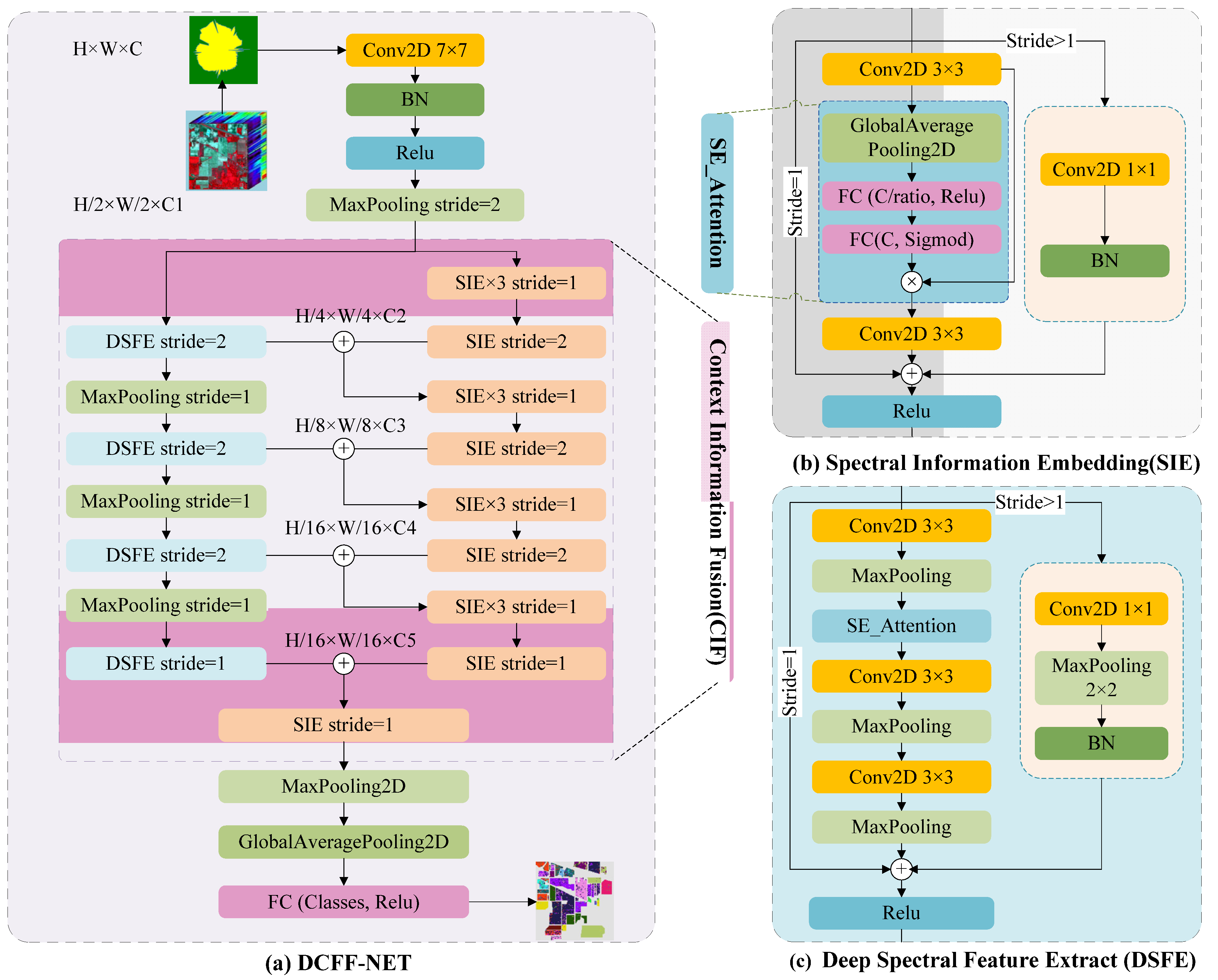
2.2.1. Spectral Information Embedding
With the advent of residual networks, the potential for deep learning network layers has substantially increased, leading to enhanced network depth and improved classification outcomes [39]. The Spectral Information Embedding (SIE) is configured as a residual block that includes a Squeeze and Excitation (SE) self-attention mechanism [55]. These residual blocks accelerate network training and mitigate challenges such as vanishing and exploding gradients. In the SIE module, the input x first undergoes a 3x3 convolution, batch normalization, and ReLU activation. Then, the SE Attention operation integrates all channels to enhance those contributing significantly to the classification task. Further convolution and batch normalization are then performed. When the stride in the input parameter is 1, the results are added back to the input layer. If the stride is greater than 1, a 1x1 convolution is applied to restore the size of the convolutional layer before adding it to the input layer to achieve the final feature encoding, which is then activated using the ReLU function. The specific structure is illustrated in Figure 2 (b).
The residual block is the basic module in the residual network model structure. The function can be expressed as follows:
where is the residual function, which can be regarded as the part that performs a nonlinear transformation on the input . The addition operation in the formula means adding the input and the output of the residual function to which obtains the output of the residual block.
Convolutional layer operations form the core of deep learning. To enhance model performance, researchers have proposed several processing methods, such as batch normalization (BN) [53], activation functions [54], maximum pooling, and average pooling. These methods improve the model's overall performance in different ways. The BN and ReLU activation functions are widely used in deep learning models. Batch normalization reduces the distribution variance across different data batches, mitigates gradient vanishing or explosion issues, and improves the training effect, generalization capability, and robustness of the deep neural network model. The ReLU activation function, known for its simplicity, speed, and effectiveness, significantly enhances model accuracy and convergence speed, demonstrating strong performance in numerous deep learning models. The formulas for these functions are defined as follows:
where is mean; is the total variance; is a small positive number to avoid division by zero. The Relu activation function is defined as follows:
where is the element value in the input tensor. For input values greater than or equal to 0, the original value is output; for input values less than 0, the output value is 0.
2.2.2. Deep Spectral Feature Extract
After each convolutional computation, batch normalization, and ReLU activation are applied, and a maximum pooling operation is employed to extract image features. This module employs a two-layer 3×3 convolutional calculation, incorporating the SE-Attention module to reconstruct the characteristics of different channels. It connects the feature map after the initial convolutional layer with that of the SE-Attention and subsequently with the feature map after the final convolutional layer to produce the ultimate feature map output of the DSFE module.
The max pooling layer preserves the most significant features and reduces the spatial dimension, diminishing the model's sensitivity to spatial location, decreasing the number of parameters, and improving computational efficiency. Max pooling methods reduce the feature map size through downsampling operations, allowing the model to learn overall features and local invariance, enhancing the model's robustness and generalization capability. For example, if the input two-dimensional feature map size is (H, W), the pooling operation employs a window of size × and a step size of . Hence, the size of the feature map output by the pooling is (, ), and the maximum pooling formula is defined as follows:
where and are the row and column index of the output feature map, respectively; and are the row and column index in the pooling window, respectively. The function represents taking the maximum value in the window.
2.2.3. Cross Entropy Loss Function and Activation Function
Cross Entropy Loss is a commonly used metric in classification tasks to evaluate the difference between predicted outcomes and actual labels. It draws from the concept of cross-entropy in information theory, assessing the performance of a model by calculating the difference between the predicted probability distribution and the true label distribution. During the training process, model parameters are refined by minimizing the cross-entropy loss function, enabling more accurate predictions of the real labels. Optimization algorithms such as Gradient Descent are frequently employed to update model parameters based on the gradient of the loss function, reducing the loss function. The mathematical expression for sparse categorical cross-entropy loss function is presented in Equation (8):
where is the probability distribution of the real label; is the predicted probability distribution of the model; is the number of categories.
The softmax activation function is employed following the fully connected layer in DCFF-NET. This function is typically utilized in the output layer of multi-classification challenges, converting the model's initial outputs into a probability distribution. Each category's probability value ranges between 0 and 1, with the total probability across all categories summing to 1. The formula for the softmax function is provided below:
where is the value of the i-th element in the input vector; is the number of categories; is the predicted probability of the i-th category.
The output from the softmax activation function delivers a probability value for each category, with the category exhibiting the highest probability designated as the final recognized category. The formula for this determination is specified below:
3. Results and Analysis
3.1. Experimental Datasets and Implementation
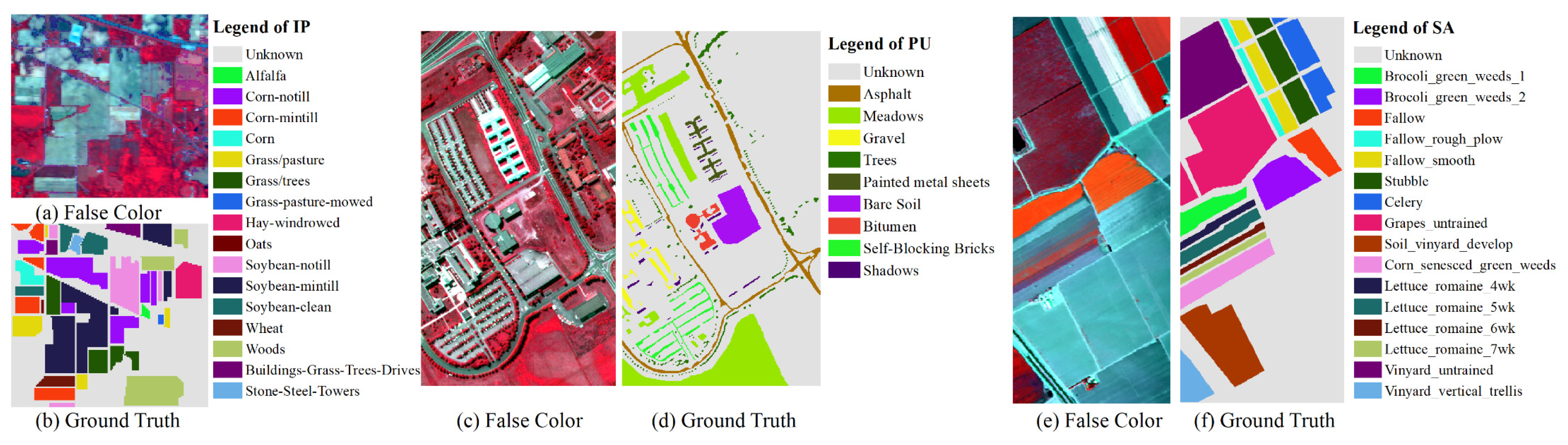
The Indian Pines (IP) Aerial hyperspectral dataset, collected by the AVIRIS sensor on June 12, 1992, encompasses an area of 2.9 km × 2.9 km in northwest Indiana. The dataset features a pixel size of 145 × 145 (21025 pixels), a spatial resolution of 20 m, a spectral range from 0.4 to 2.5 µm, and includes 16 land cover types, predominantly in agricultural regions. Originally comprising 220 bands, the dataset was refined to 200 bands after excluding 20 bands that captured atmospheric water absorption and exhibited low SNR. The retained data from these 200 bands were utilized in this experiment. Table 1 and Figure 3 (a) (b) illustrate the actual marking information of ground objects in this dataset. The sample distribution across different types is highly variable, with quantities ranging from 20 to 2455.
Aerial hyperspectral remote sensing images of Pavia University (PU) were obtained by the German airborne Reflective Optical Spectral Imager (ROSIS) on July 8, 2002, in the campus area of the University of Pavia, Italy. The spatial resolution of the data is 1.3 m, the image size is 610 x 340 pixels (207,400 pixels), and the spectral range of the image spans from 0.43 to 0.86 µm, encompassing 115 spectral channels. The dataset includes nine urban land cover types and 42,776 labeled pixels. The image on the right displays a false-color composite image of the Pavia University data and the actual overlay type of the surface. Due to noise, 12 noise bands were eliminated, leaving 103 bands to verify the performance of the proposed method. The PU dataset contains nine categories of ground objects, as shown in Figure 3 (c) (d).
The Salinas dataset (SA) consists of hyperspectral remote sensing images of the Salinas Valley region in southern California, United States, acquired by the AVIRIS sensor. The image measures 512 x 217 pixels, with a spatial resolution of 3.7 m, a spectral resolution between 9.7 and 12 nm, and a spectral range from 400 to 2500 nm. It includes 16 types of ground objects and 54,129 labeled samples. The dataset initially had 224 bands, but 20 bands affected by atmospheric water absorption and low signal-to-noise ratios were removed. The remaining 204 bands, retained after processing, are utilized in this experiment, as indicated in Figure 3 (e) (f).
Figure 3.
Figure 3. Hyperspectral dataset: Indian pines (a)(b), Pavia University (c)(d), Salinas(e)(f)
Figure 3.
Figure 3. Hyperspectral dataset: Indian pines (a)(b), Pavia University (c)(d), Salinas(e)(f)
All experiments were conducted in identical environments using two computers. The configuration for these computers was as follows: the hardware platform included an Intel Core i7-9700K (8 cores/8 threading)/i7-1100F (8 cores/16 threading) processor with 12M/16M L3-cache/, 64GB/128G DDR4 memory at 3200MHz serial speed, NVIDIA GeForce RTX 2070 GPU with 8GB DDR5/RTX 3060 GPU with 12GB DDR5 video memory, and a 1TB HDD with 7200 RPM. The software platform comprised the Windows 10 Professional operating system, Keras 2.5.0 based on TensorFlow-gpu 2.5.0, and Python 3.7.7. Models were trained using a batch size of 12, with IP models employing an Adam optimizer with a learning rate of 2×10⁻³, a decay of 1×10⁻⁴, and PU&SA models using a learning rate of 1×10⁻⁴ and a decay of 1×10⁻⁵.
3.2. Evaluation Criterion
Classification accuracy was estimated using evaluation indicators such as overall accuracy (OA), average accuracy (AA) for each category, user accuracy (UA) for each category, and kappa coefficient (KA) [1,56]. In this text, percentages represent the KA. The calculation formula is as follows:
where is the class ; (True Positive) is the number of true examples, i.e., the number of samples that are correctly classified as positive examples; (True Negative) is the number of true counterexamples, i.e., the number of samples that are correctly classified as negative examples; (False Positive) is the number of false positives. The number of examples, i.e., the number of samples that are incorrectly classified as positive examples; (False Negative) is the number of false counterexamples, that is, the number of samples that are incorrectly classified as negative examples. is the total number of categories. is the accuracy of the classifier; is the random accuracy that the classifier can achieve.
3.3. Results Analysis Based on Feature Map
Traditional Naive Bayes (NB), K-Nearest Neighbors (KNN), Random Forest (RF), and Multi-Layer Perceptron (MLP), 1D-CNN, VGG16, and ResNet50 deep learning methods were selected for comparative analysis with DCFF-NET. NB, KNN, and RF are all open-source machine learning libraries in Python. The data partitioning for random seeds was set to fixed values to achieve data recovery. NB, KNN, and RF use automatic searches (Grid Search) to select the optimal parameters with a 50% off verification method. MLP, 1D-CNN, VGG16, ResNet50, and DCFF-Net methods were implemented using TensorFlow2.5.0, and a grid search algorithm was also employed to obtain optimal parameters. When using a grid search method, important parameter selection was performed first, reducing the parameter space range and gradually narrowing the search range of the parameters based on the calculation results to improve search efficiency. This study uses different proportions of training samples for training and prediction. As the proportion of the training sample changes, the training process and performance of the model are also affected. Therefore, under different training sample proportions, the best parameter combination is sought to ensure the best performance and generalization ability of the model. The best parameters and optimal models were selected to predict and evaluate the three hyperspectral datasets. The results are depicted in Table 2.
When various classification methods use different training sample ratios, the accuracy of image prediction results increases significantly as the proportion of training samples increases. The DCFF-Net classification method performs well on the three datasets. The three different datasets exhibit higher performance than the lower training ratios in the case of 10%, 20%, and 30% training ratios. Except for the maximum value of AA, all other values achieve the maximum value and demonstrate the best classification performance overall. With 30% training samples, the OA, KA, and AA of the IP datasets are 86.68%, 85.05%, and 85.08%; the OA, KA, and AA of the PU dataset are 94.73%, 92.99%, and 92.60%; and the OA, KA, and AA of the SA dataset are 95.14%, 94.59%, and 97.48%.
3.3.1. Results of Indian Pines
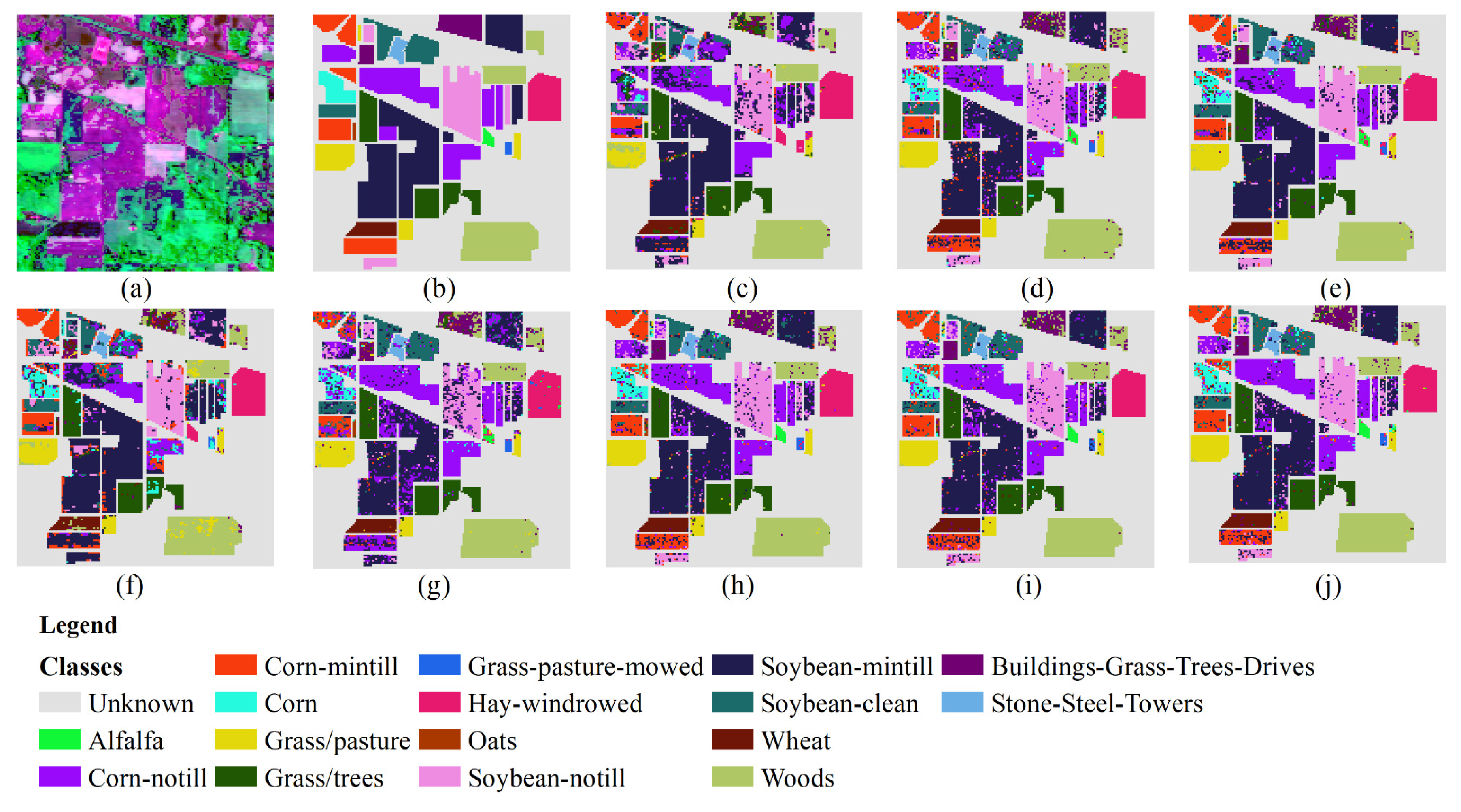
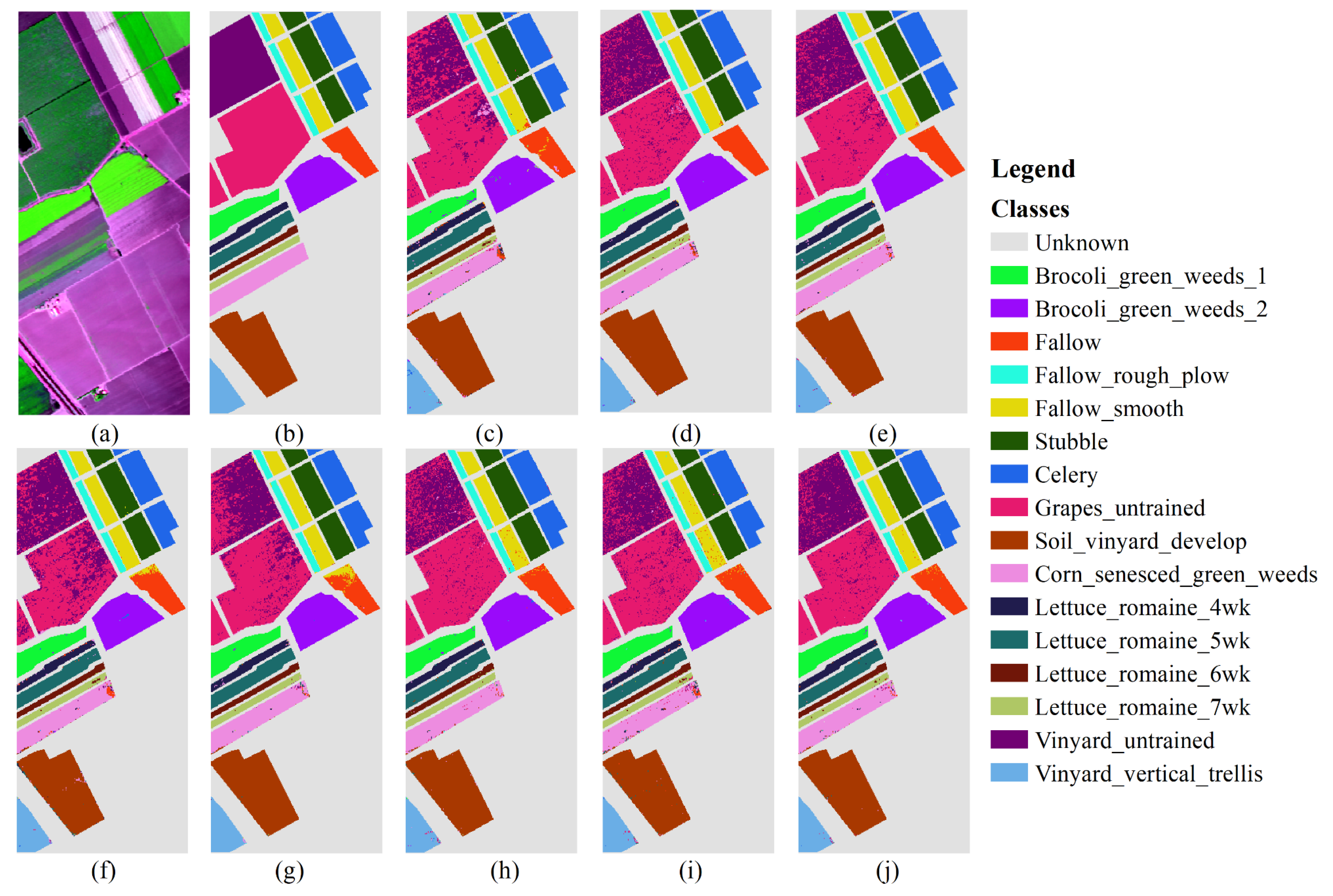
Figure 4 shows the classification result chart obtained using 30% of the training samples from the Indian Pines dataset. The UAs of each category in this dataset are listed in Table 3. It can be observed from the table that out of the 16 land types, seven types achieve the best classification effects compared to other classification methods when using the DCFF-Net classification method. The OA, KA, and AA are 86.68%, 85.04%, and 85.08%, respectively, higher than other classification methods. The classification effect of VGG16 is less than that of DCFF-Net, with OA, KA, and AA at 85.18%, 83.16%, and 83.21%, respectively. Secondly, ResNet50 also performs well. These three deep learning methods outperform other classification methods. The optimal UA values for the 16 land types are scattered across various classification methods and are not concentrated in a specific classification method. In some categories, such as Corn-no Till, Corn, Oats, and others, DCFF-Net achieves a better classification effect. The NB classification methods show significant variation in UA across different categories. For Alfalfa, Grass-Pasture-Mowed, and Oats, the UA is 0.00% due to too few samples, while the highest, Hay-Windrowed, reaches an AA of 99.40%. However, the average accuracy across the 16 categories is only 53.85%, far lower than several other methods.
Figure 4.
Predicted classification map of 30% Samples for Training. (a) Three bands false color composite. (b) Ground truth data. (c) NB. (d) KNN. (e) RF. (f) MLP. (g) 1DCNN. (h) VGG16. (i) Resnet50. (j) DCFF-NET.
Figure 4.
Predicted classification map of 30% Samples for Training. (a) Three bands false color composite. (b) Ground truth data. (c) NB. (d) KNN. (e) RF. (f) MLP. (g) 1DCNN. (h) VGG16. (i) Resnet50. (j) DCFF-NET.
3.3.2. Results of Pavia University
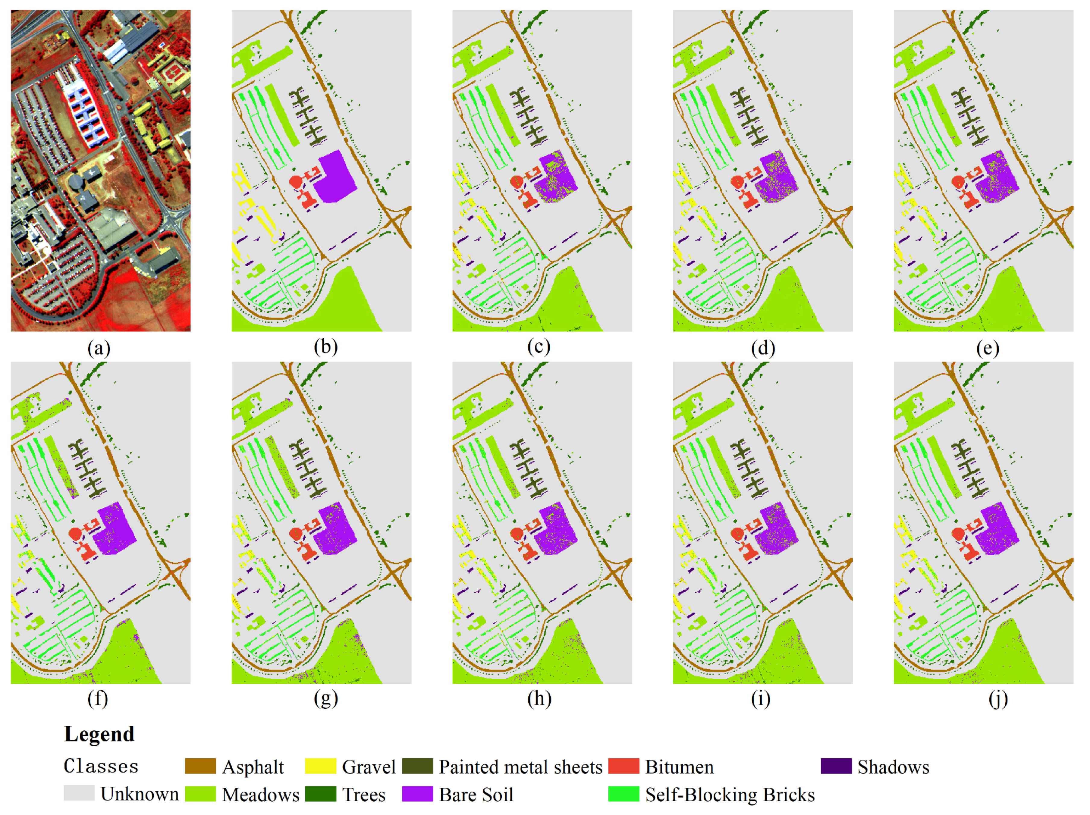
Figure 5 illustrates the classification result diagram obtained using 30% training samples on the Pavia University dataset. The OA, KA, and AA of the DCFF-Net model are 94.73%, 92.99%, and 92.60%, respectively, and these three indicators have achieved the highest classification accuracy. Trees and Bitumen's UA are the highest compared to other methods. The 1D-CNN classification result's OA is second only to DCFF-Net, reaching 93.97%. The categories Gravel, Painted Metal Sheets, Bare Soil, and Shadows are higher than other methods. For Gravel and Bitumen, no classification methods have exceeded 90.00%. In Figure 1, Gravel, Bitumen, and Self-Blocking Bricks have similar ground features, leading to generally low UA in these categories. Among all comparison methods, the KNN classification method has the lowest accuracy.
Figure 5.
Predicted classification map of 30% Samples for Training. (a) Three bands false color composite. (b) Ground truth data. (c) NB. (d) KNN. (e) RF. (f) MLP. (g) 1DCNN. (h) VGG16. (i) Resnet50. (j) DCFF-NET.
Figure 5.
Predicted classification map of 30% Samples for Training. (a) Three bands false color composite. (b) Ground truth data. (c) NB. (d) KNN. (e) RF. (f) MLP. (g) 1DCNN. (h) VGG16. (i) Resnet50. (j) DCFF-NET.
3.3.3. Results of Salinas
Figure 6 presents the classification result obtained using 30% training samples on the Salinas dataset. The number of training samples is 16,231. Table 5 shows the user accuracy (UA) of various types in SA. DCFF-Net classification OA, KA, and AA are 95.14%, 94.59%, and 97.48%, respectively, better than other comparison methods. VGG16 and ResNet50 have also achieved better classification effects, second only to DCFF-Net. Among the 16 types of land, the DCFF-Net classification results are the highest in the UA of six places. Except for the low UA in Celery, the classification accuracy in other categories is not significantly different from other classification methods. The Celery UA is extremely low. Figure 6 indicates that the characteristic graphic features of Celery and Broccoli_green_weeds_1 and Broccoli_green_weeds_2 are highly similar, making them difficult to distinguish effectively and significantly low accuracy. In the current classification methods, Grapes_untrained and Vineyard_untrained are difficult to distinguish. As shown in Table 5, the three methods—DCFF-Net, VGG16, and ResNet50—are significantly higher than other classification methods. DCFF-Net significantly increases the characteristics of similar objects, obtaining higher classification accuracy. Grapes_untrained and Vineyard_untrained achieve 98.96% and 91.71%, respectively. In other methods, the UAs of Grapes_untrained and Vineyard_untrained are lower than 90.00%, with NB, KNN, RF, MLP, 1D-CNN, and other methods achieving less than 80.00%.
Figure 6.
Predicted classification map of 30% Samples for Training. (a) Three bands false color composite. (b) Ground truth data. (c) NB. (d) KNN. (e) RF. (f) MLP. (g) 1DCNN. (h) VGG16. (i) Resnet50. (j) DCFF-NET.
Figure 6.
Predicted classification map of 30% Samples for Training. (a) Three bands false color composite. (b) Ground truth data. (c) NB. (d) KNN. (e) RF. (f) MLP. (g) 1DCNN. (h) VGG16. (i) Resnet50. (j) DCFF-NET.
The eight classification methods mentioned in the text are NB, KNN, RF, MLP, 1D-CNN, VGG16, ResNet50, and DCFF-Net. The first five methods use one-dimensional serial vector data as the model input data, while the latter three are based on two-dimensional images. The latter three methods extract image features through 2D-CNN, classifying the data into different categories. In the IP data concentration, including Corn-Min Till, Corn, Oats, and Buildings-Grass-Trees-Drives, and on the SA dataset, including Grapes_untrained and Vineyard_untrained, the accuracy of the latter three methods is significantly higher than the first five methods. This indicates that 2D-CNN can achieve better classification effects in some easily mixed categories. However, for some categories, the first five methods perform better than the latter three methods, such as Soybean-Min Till, Woods, and Stone-Steel-Towers in the IP dataset. More suitable classification methods can be selected based on these observations in practical applications.
3.4. Results Analysis Based on Pixel-Patched
An additional evaluation was conducted using the pixel-patched method to examine the classification effectiveness of DCFF-NET and assess the performance of the proposed model. The methods NB, KNN, RF, MLP, and 1D-CNN use one-dimensional vector data and cannot directly use pixels as input data. Therefore, a comparative analysis was conducted using HybridSN, 3D-CNN, and A2S2KNet models. The pixel block size was uniformly extracted at 24 × 24 × S as the input data, where S is the number of image channels, and 10% of the categories were selected as training samples. The models underwent a fine-tuning process to facilitate the utilization of VGG16 and ResNet50 models for training and testing with the provided input data. After model training was completed, the optimal model was selected for testing, using 90% of the data as test data, performing the test 10 times. The average value and standard deviation were selected as the test results, as shown in Table 6, Table 7 and Table 8. The OA and KA on the IP dataset were 98.15% and 97.89%, respectively, second only to A2S2K but higher than all other methods. The AA value of 97.73% was the highest of all methods. The OA, KA, and AA of 3D-CNN were the lowest, with values of 93.18%, 92.26%, and 94.52%, respectively. The DCFF-Net model achieved the best classification performance regarding OA, KA, and AA on the PU and SA datasets. The results on the two datasets were as follows: 99.86%, 99.82%, 99.79% and 99.98%, 99.98%, 99.94%, respectively. In addition, all comparison methods also achieved very high classification accuracy.
Figure 7.
Classification map of IP(A) PU(B)&SA(C) based on patched-based input. (a) False color composite. (b) Ground truth. (c) VGG16. (d) Resnet50. (e) 3-DCNN. (f) HybridSN. (g) A2S2K. (h) DCFF-NET.
Figure 7.
Classification map of IP(A) PU(B)&SA(C) based on patched-based input. (a) False color composite. (b) Ground truth. (c) VGG16. (d) Resnet50. (e) 3-DCNN. (f) HybridSN. (g) A2S2K. (h) DCFF-NET.
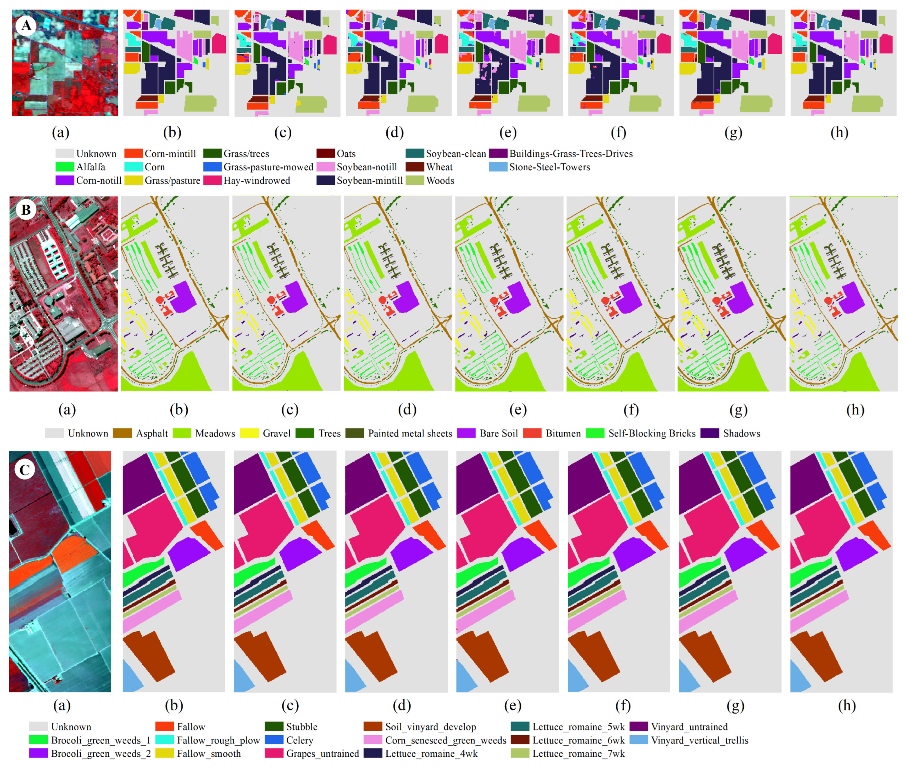
The pixel-patched block contains surrounding pixel information, specifically spectral-spatial information, which provides more discriminative cues for the target pixel. Using pixel-patched block data as the input for the model can effectively improve classification accuracy, as mentioned earlier, but it can also lead to potential label information leakage. In addition, the larger the pixel block, the more spatial information it contains; however, it will significantly increase computational complexity.
4. Discussion
4.1. Effect of Different Filling Methods
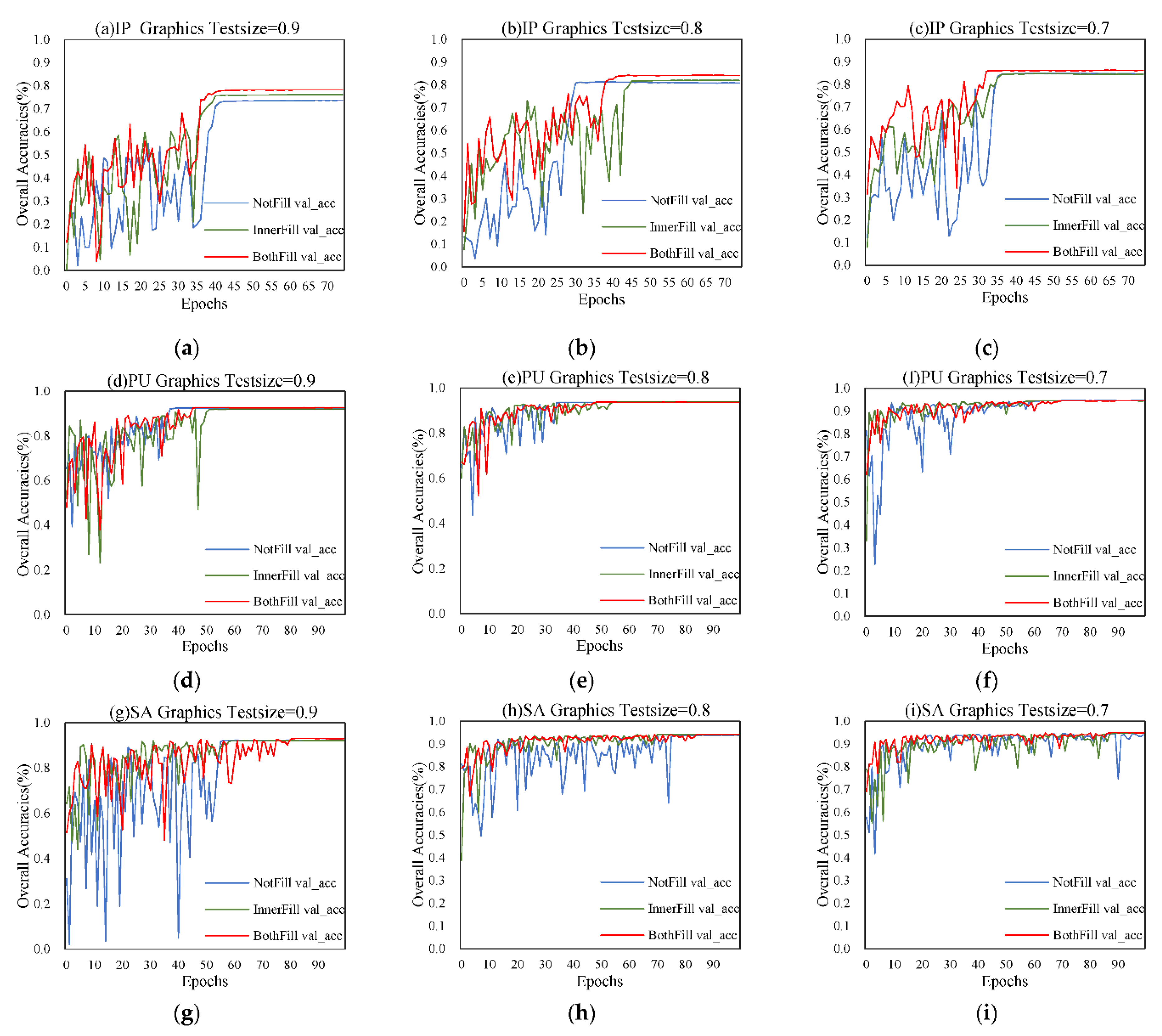
This study discusses the impact of feature map-filling characteristics on the classification accuracy of high spectral images. The spectral feature diagram employs a variety of filling methods. In Figure 8, the initial graphic (NotFill) remains unfilled, displaying a default output of white with a pixel value of 255. The second method entails internal filling in yellow, while the exterior remains unfilled (InnerFill), with the default external color being white. The third method involves internal yellow and external green filling (BothFill). The spectral characteristic graph type is determined in blue for all three methods. Through the same classification method and parameters of the three characteristic diagrams for training and verification, test on the three datasets, the IP dataset epochs is set to 75, the other two dataset epochs set to 100, 10%, 20 %, 30% of the three different proportional training samples are trained. The verification accuracy curve is illustrated in Figure 9, and the accuracy results are listed in Table 9. The results indicate that the method involving internal and external filling yields the highest classification accuracy of the feature diagram. During the training process, the convergence rates of the three characteristic diagrams are different, and the curve volatility is inconsistent. The third characteristic diagram exhibits fewer fluctuations in training accuracy, better stability, and the highest final verification accuracy. Therefore, this filling method is selected during the spectral feature diagram conversion process. The first graphic displays general fluctuations in training accuracy and a significantly slower convergence rate, whereas the second method's performance lies between the first and third methods.
Figure 8.
Different filling methods.
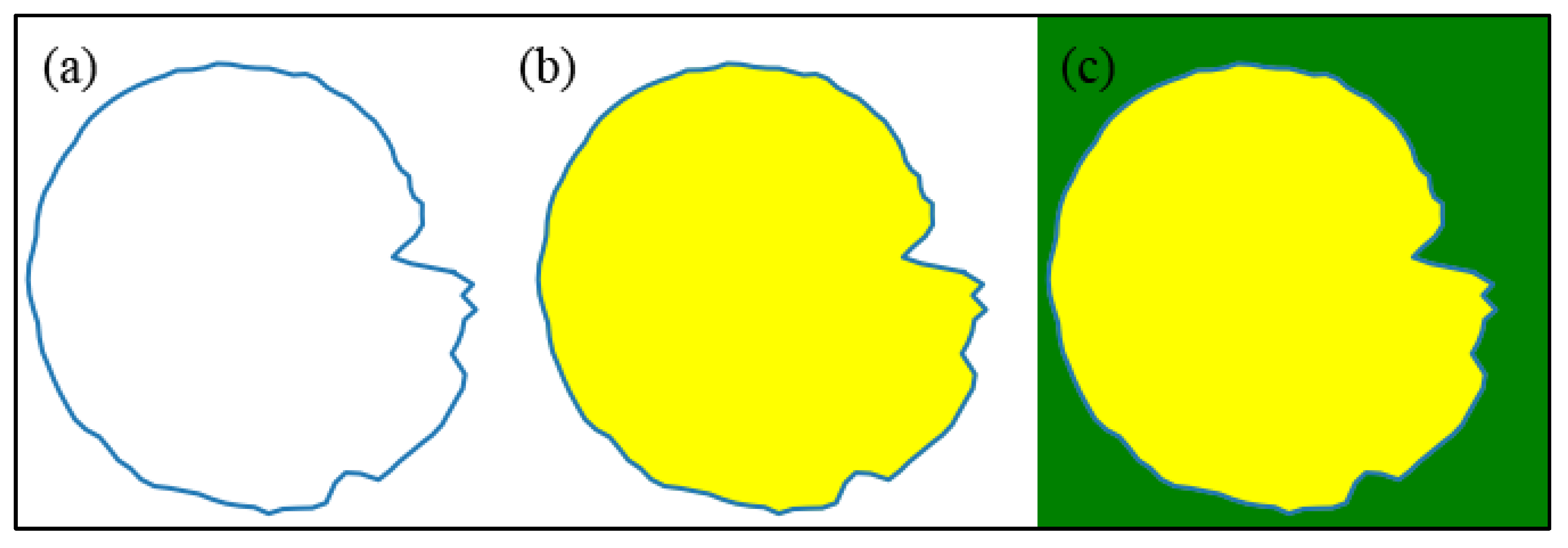
Figure 9.
Three different filling methods training accuracies curve diagrams.
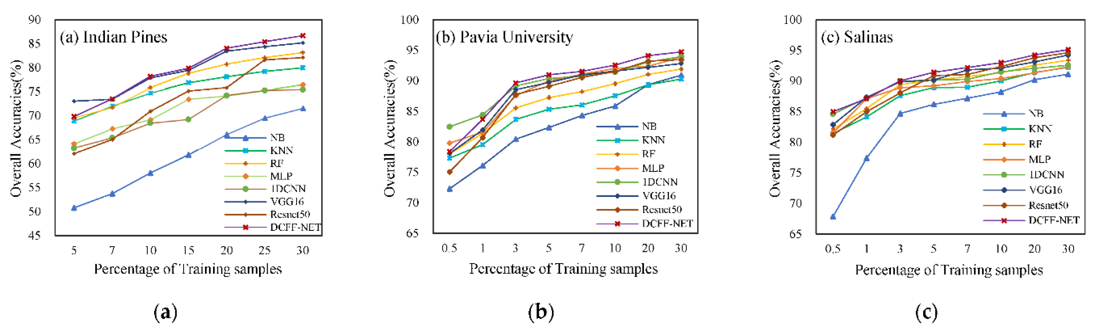
4.2. Effect of the Different Percentages of Training Samples for DCFF-NET
Different proportions of sample tag data affect classification accuracy performance significantly. Different proportions of labeled data from three datasets were selected to analyze the accuracy performance of each classification method, utilizing OA as the evaluation indicator. Proportions of 5%, 7%, 10%, 15%, 20%, 25%, and 30% from the Indian Pines dataset were chosen. In addition, 0.5%, 1%, 3%, 5%, 7%, 10%, 20%, and 30% from Pavia University and Salinas datasets were examined. Figure 10 shows that classification accuracy improves as the training sample proportion increases. For the Indian Pines dataset, the DCFF-Net classification accuracy surpasses other methods when the training sample size exceeds 7%. When the training set size is below 7%, VGG16 achieves superior overall classification accuracy. For the Pavia University and Salinas datasets, DCFF-Net outperforms other methods when the sample ratio exceeds 3%. In contrast, 1D-CNN shows better overall classification accuracy when the training sample is below 3%.
Figure 10.
Effect of the different numbers of training samples for different methods.
4.3. Ablation Analysis
The DCFF-NET model primarily utilizes the SIE and DSFE modules, with the SIE module as the core component, and integrates the DSFE module to enhance classification performance. The effectiveness of these modules was verified through individual and combined tests. When evaluating the performance of the SIE module, only the SIE module in Figure 1(a) CIF module was retained without integrating the DSFE module. In contrast, the DSFE module assessment replaced the SIE module in Figure 1(a) CIF module while retaining only the primary model for experimentation. This section replicated all experiments ten times independently with random seeds under consistent conditions. Similar to previous sections, experiments on the IP, PU, and SA datasets used three different sample proportions: 30% (Exp 1), 20% (Exp 2), and 10% (Exp 3). The final values were averaged and are displayed in Table11.

Table 11.
Comparison of ablation experiment results by different modules on three datasets. The best performing results are shown in bold.
Table 11.
Comparison of ablation experiment results by different modules on three datasets. The best performing results are shown in bold.
| Dtaset | Modules | Exp1 | Exp2 | Exp3 | |||||||
|---|---|---|---|---|---|---|---|---|---|---|---|
| SIE | DSFE | OA | KA | AA | OA | KA | AA | OA | KA | AA | |
| Indian Pines | √ | -- | 84.72±0.77 | 82.56±0.89 | 81.13±1.58 | 81.94±1.28 | 79.38±1.47 | 77.49±2.66 | 75.00±1.90 | 71.46±2.19 | 66.66±4.21 |
| -- | √ | 84.92±0.63 | 82.82±0.71 | 83.05±1.98 | 81.77±0.89 | 79.22±1.02 | 77.10±2.64 | 74.04±1.92 | 70.34±2.19 | 66.44±2.10 | |
| √ | √ | 86.06±0.37 | 84.12±0.41 | 84.41±1.07 | 83.46±0.62 | 81.01±0.71 | 79.11±2.87 | 77.56±0.95 | 74.22±1.09 | 69.9±2.87 | |
| Pavia University | √ | -- | 94.18±0.12 | 92.26±0.16 | 91.88±0.25 | 93.36±0.28 | 91.17±0.37 | 90.89±0.38 | 92.28±0.13 | 89.73±0.18 | 89.53±0.37 |
| -- | √ | 94.44±0.15 | 92.63±0.20 | 92.71±0.22 | 93.71±0.22 | 91.66±0.29 | 91.70±0.27 | 91.61±2.94 | 88.92±3.73 | 89.60±1.63 | |
| √ | √ | 94.58±0.10 | 92.67±0.14 | 92.35±0.17 | 93.85±0.18 | 91.83±0.24 | 91.51±0.31 | 92.65±0.29 | 90.23±0.39 | 89.91±0.39 | |
| Salinas | √ | -- | 95.07±0.13 | 94.51±0.14 | 97.32±0.07 | 94.25±0.10 | 93.59±0.11 | 96.77±0.10 | 92.89±0.18 | 92.08±0.20 | 95.76±0.17 |
| -- | √ | 94.92±0.22 | 94.34±0.25 | 97.37±0.15 | 94.06±0.12 | 93.39±0.13 | 96.82±0.13 | 92.71±0.19 | 91.88±0.21 | 95.93±0.28 | |
| √ | √ | 95.19±0.15 | 94.64±0.17 | 97.51±0.09 | 94.44±0.17 | 93.81±0.19 | 97.02±0.16 | 92.94±0.29 | 92.13±0.32 | 95.98±0.18 | |
Under three experimental conditions, the fusion of the SIE and DSFE modules enhanced classification results compared to individual modules. On the IP dataset, the fused classification results for Experiment 1 were as follows: OA 86.06%, KA 84.12%, and AA 84.11%. The fused model showed improvements of 1.14% in OA, 1.30% in KA, and 1.35% in AA over the DSFE module. Compared to the SIE module, improvements were 1.34% in OA, 1.56% in KA, and 3.28% in AA. The fused model also exhibited lower variance, indicating a more stable performance. Significant improvements in classification accuracy were observed under other experimental conditions as well. The improvement in classification results from the fused model on the PU and SA datasets was less pronounced than that on the IP dataset. For Experiment 1, the OA and KA of the PU dataset improved by only 0.14% and 0.04%, respectively, compared to the DSFE, with a slight decrease in AA. Compared to the SIE, the OA, KA, and AA improved by 0.40%, 0.41%, and 0.47%, respectively. For the SA dataset, the improvements were 0.27% in OA, 0.30% in KA, and 0.14% in AA compared to the DSFE, and 0.12%, 0.07%, and 0.19% compared to the SIE.
5. Conclusion
This study employs a novel approach by transforming all pixels in hyperspectral images into standardized spectral feature maps using polar coordinates. Unlike methods that rely on cube pixel patches, this approach utilizes individual pixel spectral information without considering spatial adjacency. These feature maps serve as input data for training and prediction using the proposed DCFF-Net model. The DCFF-Net includes core functionality modules: SIE, DSFE, and CIF. The CIF module achieves deep integration of the SIE and DSFE modules, effectively enhancing the model's performance. This study compares the model with other advanced classification methods using polar coordinate feature maps and pixel blocks, demonstrating its classification performance. After converting the hyperspectral pixels into polar coordinate feature maps, the process enhances the image features but also increases the data volume, which raises the computational load of the model to a certain extent, necessitating additional computational resources. Future research will focus on enhancing the model's overall performance by reducing the data's computational load.
Author Contributions
Formal analysis, Chen Zhijie, Wang Yuan and Wang Xiaoyan; Funding acquisition, Wang Xinsheng; Investigation, Chen Zhijie; Methodology, Chen Zhijie, Chen Yu, Wang Yuan and Wang Xinsheng; Project administration, Wang Xinsheng; Software, Chen Zhijie and Chen Yu; Validation, Chen Zhijie, Chen Yu, Wang Yuan and Wang Xiaoyan; Visualization, Chen Zhijie, Chen Yu and Xiang Zhouru; Writing – original draft, Chen Zhijie, Chen Yu, Wang Yuan and Wang Xiaoyan; Writing – review & editing, Chen Zhijie, Chen Yu, Wang Yuan and Xiang Zhouru.
Funding
This research was funded by the “Special projects for technological innovation in Hubei”(2018ABA078): “Research and demonstration of precision agricultural monitoring technology based on sky and earth cooperative observation”; Open Fund of “Hubei Key Laboratory of Regional Development and Environmental Response, Hubei University”(2019(B)001): the “Research on Classification Method of Hyperspectral Remote Sensing Data Based on Graph-Spatial Features”.
Data Availability Statement
Data can be provided upon request.
Conflicts of Interest
The authors declare no conflict of interest.
References
- Plaza, A., Benediktsson, J. A., & Boardman, J. W. Recent advances in techniques for hyperspectral image processing. Remote sensing of environment 2009, 113, S110–S122. [Google Scholar] [CrossRef]
- Ghamisi, P., Couceiro, M. S., & Benediktsson, J. A. Deep learning-based classification of hyperspectral data. IEEE Trans. Geosci. Remote Sens. 2017, 55, 2383–2395. [Google Scholar]
- Liu, B., Zhang, L., Zhang, L., & Du, Q. Hyperspectral image classification using deep pixel-pair features. IEEE Trans. Geosci. Remote Sens. 2015, 53, 3658–3668. [Google Scholar]
- Belhumeur, P. N. , Hespanha, J. P., & Kriegman, D. J. Eigenfaces vs. fisherfaces: Recognition using class specific linear projection. IEEE Transactions on Pattern Analysis and Machine Intelligence. 1997, 19(7), 711-720.
- Tan, S. , Chen, X. , & Zhang, D. Kernel discriminant analysis for face recognition. IEEE Transactions on Pattern Analysis and Machine Intelligence. 2011, 33(11), 2106–2112. [Google Scholar]
- Li, Y. , Chen, Y., & Jiang, J. A Novel KNN Classifier Based on Multi-Feature Fusion for Hyperspectral Image Classification. Remote Sensing 2020, 12, 745. [Google Scholar]
- Li, X. , & Liang, Y. An Improved KNN Algorithm for Intrusion Detection Based on Feature Selection and Data Augmentation. IEEE Access. 2021, 9, 17132–17144. [Google Scholar]
- Domingos, P. , & Pazzani, M. On the optimality of the simple Bayesian classifier under zero-one loss. Machine learning. 1997, 29, 103-130.
- Zhang, H. , & Wang, X. A survey on naive Bayes classifiers. Neurocomputing. 2020, 399, 14–23. [Google Scholar]
- J. Li, J. M. J. Li, J. M. Bioucas-Dias, and A. Plaza, “Spectral–spatial hyperspectral image segmentation using subspace multinomial logistic regression and Markov random fields,” IEEE Trans. Geosci. Remote Sens. 2012, 50, 809–823.
- Mo, Y. , Li, M., & Liu, Y. Multinomial logistic regression with pairwise constraints for multi-label classification. IEEE Access. 2020, 8, 74005-74016.
- Zhang, C. , & Li, J. Multinomial logistic regression with manifold regularization for image classification. Pattern Recognition Letters. 2021, 139, 55–63. [Google Scholar]
- Osuna, E. , Freund, R., & Girosi, F. Support vector machines: Training and applications. Neural Networks. 1997, 10, 631-642.
- F. Melgani and L. Bruzzone, “Classification of hyperspectral remote sensing images with support vector machines,” IEEE Trans. Geosci. Remote Sens. 2004, 40, 1778–1790.
- Wang, L. , Li, X., & Zhang, L. Support vector machines for image classification: A comprehensive review. Neurocomputing. 2016, 191, 1-9.
- Plaza, A. , Benediktsson, J. A., & Boardman, J. W. Recent advances in techniques for hyperspectral image processing. Remote sensing of environment. 2009, 113, S110-S122.
- Jia K, Li Q Z, Tian Y C, et al. A review of classification methods of remote sensing imagery[J]. Spectroscopy and Spectral Analysis. 2011, 31, 2618-2623.
- Liu, S. , Li, T., & Sun, Z. Discrimination of tea varieties using hyperspectral data based on wavelet transform and partial least squares-discriminant analysis. Food Chemistry. 2020, 325, 126914.
- He, L., Huang, W., & Zhang, X. Hyperspectral image classification with principal component analysis and support vector machine. Neurocomputing 2015, 149, 962–971. [Google Scholar]
- Zhang, J., Wang, X., & Gao, S. Fractal feature extraction of hyperspectral images using wavelet transform. In Proceedings of the 2nd International Conference on Image, Vision and Computing (ICIVC). 2018; pp. 901–905.
- Cheng, H. , Zhang, Y. , & Yang, Z. Spectral feature extraction based on key point detection and clustering algorithm. IEEE Access. 2019, 7, 43100–43107. [Google Scholar]
- Huang, H. , Chen, X. , & Guo, L. A novel method for spectral angle classification based on the support vector machine. PLOS ONE. 2020, 15, e0237772. [Google Scholar]
- Wu, D. , Zhang, L., & Shen, X. A spectral curve matching algorithm based on dynamic programming and frequency-domain filtering. IEEE Trans. Geosci. Remote Sens. 2021, 59, 4293-4307.
- Wang, Y. , & Wang, C. Spectral curve shape index: A new spectral feature for hyperspectral image classification. Journal of Applied Remote Sensing. 2021, 15, 016524.
- Huang, J. , Zhang, J. , & Li, Y. Discrimination of tea varieties using near infrared spectroscopy and chemometrics. Journal of Food Engineering. 2015, 144, 75–80. [Google Scholar]
- Liu, S. , Li, T., & Sun, Z. Discrimination of tea varieties using hyperspectral data based on wavelet transform and partial least squares-discriminant analysis. Food Chemistry. 2020, 325, 126914.
- Tao, Y. , Liu, F., & Pan, M. Rapid identification of intact paddy rice varieties using near-infrared spectroscopy and chemometric analysis. Journal of Cereal Science. 2015, 62, 59-64.
- Schmidhuber, J. Deep learning in neural networks: An overview. Neural Networks. 2015, 61, 85–117. [Google Scholar] [PubMed]
- LeCun, Y., Bengio, Y., & Hinton, G. Deep learning. nature. nature 2015, 521, 436–444. [Google Scholar] [CrossRef] [PubMed]
- LeCun, Y. , Bottou, L., Bengio, Y., & Haffner, P. Gradient-based learning applied to document recognition. Proceedings of the IEEE. 1998, 86, 2278-2324.
- Hinton, G. E. Learning multiple layers of representation. Trends in Cognitive Sciences. 2007, 11, 428–434. [Google Scholar] [CrossRef]
- Hinton, G. E. , Osindero, S. , & Teh, Y. W. A fast learning algorithm for deep belief nets. Neural computation. 2006, 18, 1527–1554. [Google Scholar]
- Krizhevsky, A., Sutskever, I., & Hinton, G. E. ImageNet classification with deep convolutional neural networks. In Advances in neural information processing systems. 2012, 1097–1105.
- Graves, A. , Mohamed, A. R., & Hinton, G. E. Speech recognition with deep recurrent neural networks. In IEEE international conference on acoustics, speech and signal processing. 2013, 6645-6649.
- Mikolov, T. , Sutskever, I. , Chen, K., Corrado, G. S., & Dean, J. Distributed representations of words and phrases and their compositionality. In Advances in neural information processing systems. 2013, 3111–3119. [Google Scholar]
- Simonyan, K. , & Zisserman, A. Very deep convolutional networks for large-scale image recognition. International Journal of Computer Vision. 2015, 113, 136-158.
- Chatfield, K., Simonyan, K., Vedaldi, A., & Zisserman, A. Return of the devil in the details: Delving deep into convolutional nets. In Proceedings of the British Machine Vision Conference (BMVC). 2014; 1–12.
- Szegedy, C., Liu, W., Jia, Y., Sermanet, P., Reed, S., Anguelov, D, & Rabinovich, A. Going deeper with convolutions. In Proceedings of the IEEE conference on computer vision and pattern recognition. 2015; 1–9.
- He, K., Zhang, X., Ren, S., & Sun, J. Deep residual learning for image recognition. In Proceedings of the IEEE conference on computer vision and pattern recognition. 2016, 770–778.
- He, K., Zhang, X., Ren, S., & Sun, J. Identity mappings in deep residual networks. In European Conference on Computer Vision (ECCV). 2016, 630–645. [Google Scholar]
- Xie, S., Girshick, R., Dollár, P., Tu, Z., & He, K. Aggregated residual transformations for deep neural networks. Proceedings of the IEEE conference on computer vision and pattern recognition. 2017, 1492–1500.
- Zhang, H. , Wu, C., Zhang, J., Zhu, Y., Zhang, Z., Lin, H.,... & Sun, Y. ResNeSt: Split-Attention Networks. IEEE/CVF Conference on Computer Vision and Pattern Recognition. 2020, 163-172.
- Wei, H. , Yangyu, H., Li, W., Fan, Z., & Hengchao, L. Deep convolutional neural networks for hyperspectral image classification. Journal of Sensors, 2015, 1-12.
- J. Mao, W. J. Mao, W. Xu, Y. Yang, J. Wang, Z. Huang, and A. Yuille, Deep Captioning with Multimodal Recurrent Neural Networks (m-RNN). 2014; arXiv:1412.6632. [Google Scholar]
- S. K. Roy, G. S. K. Roy, G. Krishna, S. R. Dubey, and B. B. Chaudhuri, Hybridsn: Exploring 3-d–2-d cnn feature hierarchy for hyperspectral image classification, IEEE Geoscience and Remote Sensing Letters. 2019, 17, 277–281.
- A. B. Hamida, A. A. B. Hamida, A. Benoit, P. Lambert, and C. B. Amar, 3-d deep learning approach for remote sensing image classification, IEEE Trans. Geosci. Remote Sens. 2018, 56,4420 4434.
- Z. Zhong, J. Z. Zhong, J. Li, Z. Luo, and M. Chapman, Spectralspatial residual network for hyperspectral image classification: A 3-d deep learning framework, IEEE Trans. Geosci. Remote Sens. 2018, 56, 847-858.
- Qing,Y.; Huang,Q.; Feng, L.; Qi, Y.; Liu, W. Multiscale Feature Fusion Network Incorporating 3D Self-Attention for Hyperspectral Image Classification. Remote Sens. 2022, 14, 742.
- Qing, Y.; Liu, W. Hyperspectral image classification based on multi-scale residual network with attention mechanism. Remote Sens. 2021, 13, 335. [Google Scholar] [CrossRef]
- Y. Chen, H. Y. Chen, H. Jiang, C. Li, X. Jia, and P. Ghamisi, Deep Feature Extraction and Classification of Hyperspectral Images Based on Convolutional Neural Networks, IEEE Trans. Geosci. Remote Sens.2016, 54, 6232–6251.
- Wu, J.; Sun, X.; Qu, L.; Tian, X.; Yang, G. Learning Spatial–Spectral-Dimensional-Transformation-Based Features for Hyperspectral Image Classification. Appl. Sci. 2023, 13, 8451. [Google Scholar] [CrossRef]
- Wei, Y. , Feng, J., Liang, X., Cheng, M.-M., Zhao, Y., & Yan, S. Object Region Mining with Adversarial Erasing: A Simple Classification to Semantic Segmentation Approach. Proceedings of the IEEE Conference on Computer Vision and Pattern Recognition. 2017.
- S. Ioffe and C. Szegedy. Batch normalization: Accelerating deep network training by reducing internal covariate shift. In ICML, 2015.
- He, K., Zhang, X., Ren, S., & Sun, J. Delving deep into rectifiers: Surpassing human-level performance on ImageNet classification. In Proceedings of the IEEE International Conference on Computer Vision (ICCV). 2015; 1026–1034. [Google Scholar]
- Jie Hu, Li Shen, Gang Sun. Squeeze-and-Excitation Networks. In Proceedings of the IEEE Conference on Computer Vision and Pattern Recognition (CVPR), 2018, 7132-7141.
- Bhattacharyya, C.; Kim, S. Black Ice Classification with Hyperspectral Imaging and Deep Learning. Appl. Sci. 2023, 13, 11977. [Google Scholar] [CrossRef]
Figure 1.
Feature maps of Three Datasets . (a) Indian pines; (b) Pavia University; (c) Salinas.
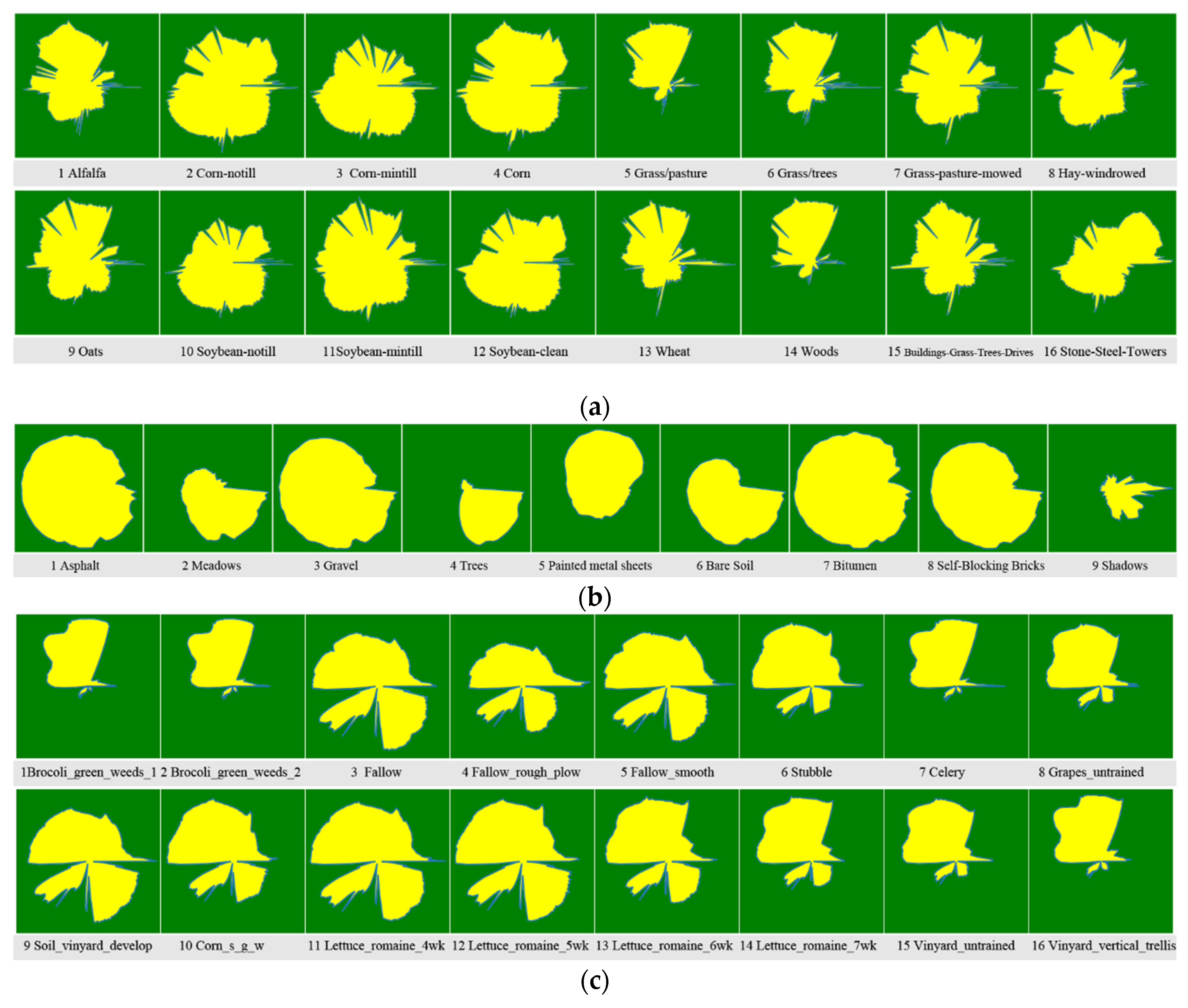
Table 1.
Detailed information of three datasets.
| Classes | Indian Pines | Salinas | Pavia University | |||
|---|---|---|---|---|---|---|
| Names | Samples | Names | Samples | Names | Samples | |
| 1 | Alfalfa | 46 | Brocoli_green_weeds_1 | 2009 | Asphalt | 6631 |
| 2 | Corn-no till | 1428 | Brocoli_green_weeds_2 | 3726 | Meadows | 18649 |
| 3 | Corn-min till | 830 | Fallow | 1976 | Gravel | 2099 |
| 4 | Corn | 237 | Fallow_rough_plow | 1394 | Trees | 3064 |
| 5 | Grass-pasture | 483 | Fallow_smooth | 2678 | Painted metal sheets | 1345 |
| 6 | Grass-trees | 730 | Stubble | 3959 | Bare Soil | 5029 |
| 7 | Grass-pasture-mowed | 28 | Celery | 3579 | Bitumen | 1330 |
| 8 | Hay-windrowed | 478 | Grapes_untrained | 11271 | Self-Blocking Bricks | 3682 |
| 9 | Oats | 20 | Soil_vinyard_develop | 6203 | Shadows | 947 |
| 10 | Soybean-no till | 972 | Corn_senesced_green_weeds | 3278 | -- | -- |
| 11 | Soybean-min till | 2455 | Lettuce_romaine_4wk | 1068 | -- | -- |
| 12 | Soybean-clean | 593 | Lettuce_romaine_5wk | 1927 | -- | -- |
| 13 | Wheat | 205 | Lettuce_romaine_6wk | 916 | -- | -- |
| 14 | Woods | 1265 | Lettuce_romaine_7wk | 1070 | -- | -- |
| 15 | Buildings-Grass-Trees-Drives | 386 | Vinyard_untrained | 7268 | -- | -- |
| 16 | Stone-Steel-Towers | 93 | Vinyard_vertical_trellis | 1807 | -- | -- |
| Total Samples | 10249 | 54129 | 42956 | |||
Table 2.
Accuracies of each method with different training samples on three datasets.
| Methods | Train /Test |
IP | PU | SA | ||||||
|---|---|---|---|---|---|---|---|---|---|---|
| OA | KA | AA | OA | KA | AA | OA | KA | AA | ||
| NB | 30%/70% | 71.58 | 66.96 | 53.85 | 90.91 | 87.79 | 87.39 | 91.13 | 90.10 | 94.22 |
| KNN | 79.98 | 77.12 | 79.09 | 90.28 | 86.94 | 88.29 | 92.24 | 91.36 | 96.10 | |
| RF | 83.17 | 80.66 | 73.67 | 91.91 | 89.17 | 89.39 | 93.39 | 92.63 | 96.39 | |
| MLP | 77.65 | 74.52 | 77.12 | 93.88 | 91.86 | 90.31 | 92.31 | 91.43 | 95.67 | |
| 1DCNN | 79.90 | 76.94 | 76.65 | 93.97 | 92.00 | 92.42 | 93.34 | 92.58 | 96.91 | |
| VGG16 | 85.18 | 83.16 | 83.21 | 92.19 | 89.64 | 89.56 | 94.25 | 93.59 | 96.66 | |
| Resnet50 | 82.13 | 79.60 | 77.71 | 93.44 | 91.28 | 90.49 | 94.62 | 94.01 | 97.23 | |
| DCFF-NET | 86.68 | 85.04 | 85.08 | 94.73 | 92.99 | 92.60 | 95.14 | 94.59 | 97.48 | |
| NB | 20%/80% | 66.14 | 60.52 | 48.63 | 89.36 | 85.61 | 85.24 | 90.21 | 89.09 | 93.37 |
| KNN | 78.12 | 75.00 | 76.38 | 89.34 | 85.61 | 87.25 | 91.38 | 90.40 | 95.54 | |
| RF | 80.75 | 77.85 | 66.60 | 91.04 | 87.95 | 88.05 | 92.60 | 91.75 | 95.90 | |
| MLP | 75.20 | 71.53 | 71.95 | 92.37 | 89.95 | 90.56 | 91.34 | 90.34 | 94.60 | |
| 1DCNN | 73.88 | 69.59 | 68.63 | 93.07 | 90.82 | 89.79 | 92.33 | 91.43 | 96.29 | |
| VGG16 | 83.44 | 81.12 | 83.25 | 92.83 | 90.48 | 89.64 | 92.55 | 91.68 | 95.73 | |
| Resnet50 | 75.84 | 72.44 | 73.64 | 93.23 | 91.00 | 90.89 | 93.80 | 93.10 | 96.48 | |
| DCFF-NET | 84.05 | 81.77 | 79.90 | 94.11 | 92.18 | 91.86 | 94.24 | 93.58 | 96.81 | |
| NB | 10%/90% | 58.05 | 50.08 | 40.93 | 85.85 | 80.67 | 79.52 | 88.22 | 86.86 | 91.49 |
| KNN | 74.76 | 71.20 | 70.97 | 87.53 | 83.12 | 85.01 | 90.03 | 88.90 | 94.42 | |
| RF | 75.87 | 72.27 | 60.42 | 89.52 | 85.86 | 85.79 | 91.31 | 90.31 | 94.93 | |
| MLP | 69.20 | 64.93 | 60.60 | 92.02 | 89.40 | 89.34 | 90.41 | 89.35 | 94.91 | |
| 1DCNN | 69.36 | 64.98 | 64.48 | 92.71 | 90.39 | 90.85 | 91.55 | 90.58 | 94.98 | |
| VGG16 | 77.88 | 74.73 | 72.80 | 91.59 | 88.84 | 88.61 | 92.12 | 91.23 | 95.50 | |
| Resnet50 | 70.90 | 66.54 | 64.14 | 91.51 | 88.73 | 89.18 | 92.35 | 91.47 | 94.86 | |
| DCFF-NET | 78.21 | 75.07 | 84.36 | 92.56 | 90.40 | 90.39 | 93.00 | 92.20 | 95.66 | |
Table 3.
Accuracies (%) of labeled samples per class for the Indian Pines dataset.
| Classes Name | Train/Test | NB | KNN | RF | MLP | 1DCNN | VGG16 | Resnet50 | DCFF-NET |
|---|---|---|---|---|---|---|---|---|---|
| Alfalfa | 13/33 | 0.00 | 69.70 | 66.67 | 82.61 | 15.62 | 90.32 | 92.00 | 92.00 |
| Corn-no till | 428/1000 | 60.60 | 70.00 | 76.90 | 47.62 | 73.30 | 77.27 | 71.49 | 83.48 |
| Corn-min till | 249/581 | 39.07 | 65.58 | 60.24 | 70.24 | 72.98 | 86.70 | 82.30 | 84.42 |
| Corn | 71/166 | 13.25 | 59.04 | 56.02 | 70.04 | 64.46 | 80.29 | 73.03 | 86.40 |
| Grass-pasture | 144/339 | 70.80 | 93.51 | 89.09 | 83.64 | 84.62 | 96.99 | 92.57 | 98.65 |
| Grass-trees | 219/511 | 97.06 | 96.09 | 96.67 | 89.86 | 95.50 | 93.43 | 95.59 | 95.71 |
| Grass-pasture-mowed | 8/20 | 0.00 | 85.00 | 40.00 | 85.71 | 95.00 | 76.49 | 66.67 | 72.03 |
| Hay-windrowed | 143/335 | 99.40 | 98.51 | 98.81 | 96.44 | 94.03 | 92.31 | 91.43 | 92.86 |
| Oats | 6/14 | 0.00 | 71.43 | 21.43 | 25.00 | 78.57 | 80.91 | 80.30 | 83.78 |
| Soybean-no till | 291/681 | 66.81 | 79.15 | 82.09 | 73.97 | 60.15 | 72.41 | 67.08 | 77.41 |
| Soybean-min till | 736/1719 | 87.32 | 82.32 | 90.87 | 82.00 | 84.47 | 66.46 | 61.63 | 75.00 |
| Soybean-clean | 177/416 | 38.22 | 62.50 | 69.71 | 77.07 | 72.53 | 92.26 | 92.66 | 92.66 |
| Wheat | 61/144 | 93.75 | 100.00 | 95.83 | 99.51 | 98.60 | 97.60 | 94.48 | 96.84 |
| Woods | 379/886 | 97.97 | 91.99 | 95.03 | 97.08 | 94.13 | 72.22 | 63.64 | 81.82 |
| Buildings-Grass-Trees-Drives | 115/271 | 16.97 | 54.24 | 57.56 | 60.62 | 56.30 | 98.58 | 99.70 | 100.00 |
| Stone-Steel-Towers | 27/66 | 80.30 | 86.36 | 81.82 | 92.47 | 86.15 | 57.14 | 18.75 | 56.25 |
| OA | 3067/7182 | 71.58 | 79.98 | 83.17 | 77.65 | 79.90 | 85.18 | 82.13 | 86.68 |
| KA | 66.96 | 77.12 | 80.66 | 74.52 | 76.94 | 83.16 | 79.60 | 85.04 | |
| AA | 53.85 | 79.09 | 73.67 | 77.12 | 76.65 | 83.21 | 77.71 | 85.08 |
Table 4.
Accuracies (%) of labeled samples per class for the Pavia University dataset
| Classes Name | Train/Test | NB | KNN | RF | MLP | 1DCNN | VGG16 | Resnet50 | DCFF-NET |
|---|---|---|---|---|---|---|---|---|---|
| Asphalt | 1989/4642 | 90.69 | 89.19 | 92.20 | 92.45 | 94.64 | 93.08 | 94.46 | 93.84 |
| Meadows | 5594/13055 | 98.47 | 97.88 | 97.94 | 97.82 | 97.65 | 96.51 | 97.36 | 97.54 |
| Gravel | 629/1470 | 66.87 | 74.56 | 74.15 | 65.66 | 88.16 | 71.34 | 73.13 | 77.70 |
| Trees | 919/2145 | 90.26 | 88.21 | 91.93 | 95.22 | 94.03 | 91.01 | 95.44 | 96.00 |
| Painted metal sheets | 403/942 | 99.15 | 99.47 | 99.15 | 99.26 | 100.00 | 99.37 | 99.38 | 99.17 |
| Bare Soil | 1508/3521 | 74.07 | 69.33 | 77.08 | 90.62 | 92.53 | 89.75 | 90.58 | 92.02 |
| Bitumen | 399/931 | 77.23 | 87.76 | 81.95 | 75.68 | 86.47 | 80.53 | 77.63 | 88.05 |
| Self-Blocking Bricks | 1104/2578 | 89.91 | 88.17 | 90.11 | 93.15 | 78.27 | 84.75 | 87.01 | 88.35 |
| Shadows | 284/663 | 99.85 | 100.00 | 100.00 | 99.25 | 100.00 | 99.70 | 99.39 | 99.70 |
| OA | 12829/29947 | 90.91 | 90.28 | 91.91 | 92.70 | 93.97 | 92.19 | 93.44 | 94.73 |
| KA | 87.79 | 86.94 | 89.17 | 90.22 | 92.00 | 89.64 | 91.28 | 92.99 | |
| AA | 87.39 | 88.29 | 89.39 | 89.90 | 92.42 | 89.56 | 90.49 | 92.60 |
Table 5.
Accuracies (%) of labeled samples per class for the Salinas dataset(30%Train)
| Classes Name | Train/Test | NB | KNN | RF | MLP | 1DCNN | VGG16 | Resnet50 | DCFF-NET |
|---|---|---|---|---|---|---|---|---|---|
| Brocoli_green_weeds_1 | 602/1407 | 97.51 | 99.29 | 99.93 | 99.36 | 100.00 | 99.86 | 99.79 | 99.59 |
| Brocoli_green_weeds_2 | 1117/2609 | 99.16 | 99.92 | 99.96 | 99.43 | 99.96 | 96.18 | 95.25 | 96.82 |
| Fallow | 592/1384 | 96.46 | 99.93 | 99.42 | 91.04 | 99.42 | 98.43 | 99.08 | 98.69 |
| Fallow_rough_plow | 418/976 | 99.08 | 99.39 | 99.39 | 99.08 | 99.18 | 98.12 | 99.41 | 99.48 |
| Fallow_smooth | 803/1875 | 96.48 | 98.51 | 98.77 | 98.72 | 99.20 | 94.71 | 99.06 | 99.22 |
| Stubble | 1187/2772 | 99.42 | 99.64 | 99.75 | 99.89 | 99.96 | 98.67 | 98.96 | 98.45 |
| Celery | 1073/2506 | 99.20 | 99.60 | 99.68 | 99.80 | 99.88 | 80.96 | 81.36 | 80.64 |
| Grapes_untrained | 3381/7890 | 87.93 | 85.02 | 89.91 | 79.62 | 86.43 | 97.17 | 98.65 | 98.96 |
| Soil_vinyard_develop | 1860/4343 | 99.06 | 99.52 | 99.36 | 98.83 | 99.93 | 98.66 | 99.77 | 99.92 |
| Corn_senesced_green_weeds | 983/2295 | 91.42 | 94.12 | 94.51 | 92.81 | 98.30 | 97.33 | 97.59 | 98.76 |
| Lettuce_romaine_4wk | 320/748 | 89.44 | 97.86 | 95.99 | 98.40 | 98.93 | 99.39 | 99.28 | 99.17 |
| Lettuce_romaine_5wk | 578/1349 | 99.56 | 99.85 | 99.41 | 85.17 | 99.48 | 98.97 | 99.05 | 99.31 |
| Lettuce_romaine_6wk | 274/642 | 97.82 | 98.75 | 98.44 | 97.66 | 99.38 | 99.78 | 99.74 | 99.93 |
| Lettuce_romaine_7wk | 321/749 | 92.79 | 96.66 | 97.06 | 97.46 | 97.33 | 99.88 | 99.68 | 99.52 |
| Vinyard_untrained | 2180/5088 | 65.33 | 71.29 | 72.27 | 78.83 | 73.92 | 88.61 | 89.51 | 91.71 |
| Vinyard_vertical_trellis | 542/1265 | 96.92 | 98.26 | 98.42 | 98.10 | 99.21 | 99.82 | 99.45 | 99.58 |
| OA | 16231/37898 | 91.13 | 92.24 | 93.39 | 91.13 | 93.34 | 94.25 | 94.62 | 95.14 |
| KA | 90.10 | 91.36 | 92.63 | 90.14 | 92.58 | 93.59 | 94.01 | 94.59 | |
| AA | 94.22 | 96.10 | 96.39 | 94.64 | 96.91 | 96.66 | 97.23 | 97.48 |
Table 6.
Accuracies of Indian pines dataset.
| Classes Name | Train/Test | VGG16 | Resnet50 | 3-DCNN | HybridSN | A2S2K | DCFF-NET |
|---|---|---|---|---|---|---|---|
| Alfalfa | 4/42 | 100.00±0.00 | 100.00±0.00 | 100.00±0.00 | 100.00±0.00 | 93.5±7.040 | 98.6±1.15 |
| Corn-no till | 142/1286 | 96.68±0.19 | 97.72±0.10 | 90.86±0.20 | 94.51±0.20 | 97.45±2.69 | 98.03±0.14 |
| Corn-min till | 83/747 | 89.95±0.26 | 96.48±0.20 | 78.99±0.29 | 93.47±0.29 | 97.54±1.63 | 99.62±0.08 |
| Corn | 23/214 | 89.69±0.63 | 84.84±0.61 | 89.65±1.16 | 69.14±1.16 | 98.09±1.30 | 95.54±0.48 |
| Grass-pasture | 48/435 | 83.01±0.84 | 89.3±0.39 | 92.94±0.24 | 94.3±0.24 | 99.66±0.31 | 87.01±0.40 |
| Grass-trees | 73/657 | 99.08±0.10 | 97.56±0.18 | 100.00±0.00 | 99.02±0.10 | 99.28±0.91 | 100.00±0.00 |
| Grass-pasture-mowed | 2/26 | 100.00±0.00 | 100.00±0.00 | 88.54±0.00 | 100.00±0.00 | 90.63±13.26 | 100.00±0.00 |
| Hay-windrowed | 47/431 | 100.00±0.00 | 100.00±0.00 | 100.00±0.00 | 100.00±0.00 | 99.57±0.60 | 99.77±0.00 |
| Oats | 2/18 | 100.00±0.00 | 100.00±0.00 | 95.54±0.00 | 100.00±0.00 | 72.22±20.79 | 100.00±0.00 |
| Soybean-no till | 97/875 | 95.85±0.08 | 98.29±0.12 | 100.00±0.20 | 95.94±0.20 | 97.59±0.97 | 96.90±0.14 |
| Soybean-min till | 245/2210 | 98.63±0.08 | 99.57±0.05 | 88.44±0.08 | 96.5±0.08 | 99.11±0.51 | 99.25±0.07 |
| Soybean-clean | 59/534 | 91.56±0.32 | 95.24±0.23 | 93.28±0.40 | 89.1±0.40 | 98.52±1.32 | 95.47±0.22 |
| Wheat | 20/185 | 99.61±0.25 | 98.97±0.17 | 100.00±0.00 | 100.00±0.00 | 97.47±1.46 | 100.00±0.00 |
| Woods | 126/1139 | 96.14±0.20 | 99.82±0.00 | 99.91±0.12 | 98.9±0.12 | 99.55±0.51 | 99.84±0.03 |
| Buildings-Grass-Trees-Drives | 38/348 | 99.45±0.09 | 99.02±0.18 | 100.00±0.00 | 97.91±0.17 | 95.04±3.20 | 100.00±0.00 |
| Stone-Steel-Towers | 9/84 | 91.22±0.80 | 83.69±1.15 | 94.16±1.24 | 85.64±1.24 | 94.36±6.10 | 93.67±0.80 |
| OA | 1018/9231 | 95.82±0.075 | 97.6±0.039 | 93.18±0.069 | 95.46±0.063 | 98.29±0.345 | 98.15±0.036 |
| KA | 95.24±0.084 | 97.26±0.045 | 92.26±0.079 | 94.81±0.072 | 98.05±0.394 | 97.89±0.041 | |
| AA | 95.68±0.094 | 96.28±0.105 | 94.52±0.168 | 94.65±0.123 | 95.60±0.649 | 97.73±0.092 |
Table 7.
Accuracies of Pavia University dataset.
| Classes Name | Train/Test | VGG16 | Resnet50 | 3-DCNN | HybridSN | A2S2K | DCFF-NET |
|---|---|---|---|---|---|---|---|
| Asphalt | 663/5968 | 99.49±0.03 | 99.45±0.03 | 99.76±0.01 | 99.24±0.03 | 99.91±0.08 | 99.89±0.01 |
| Meadows | 1864/16785 | 99.97±0.01 | 99.98±0.00 | 99.95±0.01 | 99.98±0.00 | 99.97±0.02 | 99.92±0.01 |
| Gravel | 209/1890 | 99.77±0.03 | 99.66±0.03 | 99.85±0.02 | 97.49±0.09 | 99.8±0.28 | 100.00±0.00 |
| Trees | 306/2758 | 98.1±0.06 | 98.43±0.04 | 99.32±0.05 | 99.62±0.03 | 99.96±0.06 | 99.17±0.04 |
| Painted metal sheets | 134/1211 | 99.93±0.03 | 100.00±0.00 | 100.00±0.00 | 100.00±0.00 | 99.97±0.04 | 100.00±0.00 |
| Bare Soil | 502/4527 | 100.00±0.00 | 100.00±0.00 | 100.00±0.00 | 99.83±0.01 | 99.93±0.06 | 100.00±0.00 |
| Bitumen | 133/1197 | 98.71±0.11 | 98.63±0.10 | 99.35±0.10 | 96.98±0.14 | 99.97±0.04 | 99.20±0.06 |
| Self-Blocking Bricks | 368/3314 | 99.75±0.02 | 99.96±0.02 | 99.89±0.01 | 99.76±0.03 | 98.44±1.13 | 100.00±0.00 |
| Shadows | 94/853 | 99.26±0.08 | 99.14±0.09 | 99.88±0.00 | 99.89±0.04 | 99.74±0.21 | 99.91±0.05 |
| OA | 4273/38503 | 99.68±0.007 | 99.71±0.007 | 99.85±0.007 | 99.58±0.004 | 99.81±0.093 | 99.86±0.004 |
| KA | 99.58±0.009 | 99.62±0.009 | 99.80±0.009 | 99.45±0.005 | 99.75±0.123 | 99.82±0.006 | |
| AA | 99.44±0.013 | 99.47±0.016 | 99.78±0.014 | 99.20±0.017 | 99.74±0.103 | 99.79±0.011 |
Table 8.
Accuracies of Salinas dataset.
| Classes Name | Train/Test | VGG16 | Resnet50 | 3-DCNN | HybridSN | A2S2K | DCFF-NET |
|---|---|---|---|---|---|---|---|
| Brocoli_green_weeds_1 | 200/1809 | 100.00±0.00 | 100.00±0.00 | 100.00±0.00 | 100.00±0.00 | 100.00±0.00 | 100.00±0.00 |
| Brocoli_green_weeds_2 | 372/3354 | 100.00±0.00 | 100.00±0.00 | 100.00±0.00 | 100.00±0.00 | 100.00±0.00 | 100.00±0.00 |
| Fallow | 197/1779 | 100.00±0.00 | 99.89±0.02 | 99.96±0.02 | 100.00±0.00 | 100.00±0.00 | 100.00±0.00 |
| Fallow_rough_plow | 139/1255 | 99.86±0.03 | 100.00±0.00 | 100.00±0.00 | 99.92±0.00 | 99.82±0.15 | 99.94±0.03 |
| Fallow_smooth | 267/2411 | 99.88±0.01 | 99.7±0.03 | 99.88±0.02 | 99.81±0.02 | 99.95±0.04 | 99.96±0.01 |
| Stubble | 395/3564 | 99.96±0.02 | 100.00±0.00 | 100.00±0.00 | 100.00±0.00 | 100.00±0.00 | 100.00±0.00 |
| Celery | 357/3222 | 100.00±0.00 | 100.00±0.00 | 100.00±0.00 | 100.00±0.00 | 100.00±0.00 | 99.97±0.00 |
| Grapes_untrained | 1127/10144 | 100.00±0.00 | 100.00±0.00 | 99.98±0.01 | 99.96±0.01 | 99.95±0.03 | 99.99±0.00 |
| Soil_vinyard_develop | 620/5583 | 100.00±0.00 | 100.00±0.00 | 100.00±0.00 | 100.00±0.00 | 99.97±0.03 | 100.00±0.00 |
| Corn_senesced_green_weeds | 327/2951 | 99.60±0.03 | 100.00±0.00 | 99.81±0.02 | 99.83±0.04 | 99.94±0.09 | 100.00±0.00 |
| Lettuce_romaine_4wk | 106/962 | 100.00±0.00 | 100.00±0.00 | 99.51±0.05 | 100.00±0.00 | 100.00±0.00 | 99.24±0.08 |
| Lettuce_romaine_5wk | 192/1735 | 100.00±0.00 | 100.00±0.00 | 99.91±0.03 | 100.00±0.00 | 100.00±0.00 | 100.00±0.00 |
| Lettuce_romaine_6wk | 91/825 | 100.00±0.00 | 99.88±0.00 | 99.89±0.04 | 99.9±0.05 | 99.96±0.06 | 100.00±0.00 |
| Lettuce_romaine_7wk | 107/963 | 100.00±0.00 | 100.00±0.00 | 100.00±0.00 | 99.61±0.04 | 99.61±0.55 | 100.00±0.00 |
| Vinyard_untrained | 726/6542 | 99.99±0.00 | 99.82±0.02 | 100.00±0.00 | 100.00±0.00 | 99.85±0.18 | 100.00±0.00 |
| Vinyard_vertical_trellis | 180/1627 | 99.82±0.02 | 100.00±0.00 | 99.71±0.03 | 99.77±0.03 | 100.00±0.00 | 100.00±0.00 |
| OA | 5403/48726 | 99.95±0.003 | 99.96±0.003 | 99.95±0.002 | 99.95±0.003 | 99.95±0.032 | 99.98±0.002 |
| KA | 99.95±0.003 | 99.95±0.003 | 99.95±0.002 | 99.95±0.003 | 99.94±0.036 | 99.98±0.003 | |
| AA | 99.94±0.003 | 99.96±0.002 | 99.92±0.004 | 99.92±0.004 | 99.94±0.039 | 99.94±0.006 |
Table 9.
Overall Accuracies under different training sample proportions and different filling methods.
Table 9.
Overall Accuracies under different training sample proportions and different filling methods.
| Datasets | IP | PU | SA | ||||||
| Filling Method | 10% | 20% | 30% | 10% | 20% | 30% | 10% | 20% | 30% |
| NotFill | 73.74 | 80.73 | 84.62 | 92.38 | 93.62 | 94.55 | 92.34 | 93.72 | 94.07 |
| InnerFill | 76.18 | 81.89 | 84.37 | 91.90 | 93.81 | 94.44 | 92.09 | 94.17 | 94.73 |
| BothFill | 78.21 | 84.05 | 86.68 | 92.56 | 94.11 | 94.73 | 93.00 | 94.24 | 95.14 |
Table 10.
Accuracies of different percentages of training samples on three datasets.
| Dataset | Train Percentage | NB | KNN | RF | MLP | 1DCNN | VGG16 | Resnet50 | DCFF-NET |
|---|---|---|---|---|---|---|---|---|---|
| Indian pines | 5 | 50.81 | 68.96 | 69.63 | 64.19 | 63.26 | 73.03 | 62.11 | 69.84 |
| 7 | 53.75 | 72.04 | 71.74 | 67.32 | 65.37 | 73.43 | 65.03 | 73.51 | |
| 10 | 58.05 | 74.76 | 75.87 | 69.20 | 68.44 | 77.88 | 70.90 | 78.21 | |
| 15 | 61.83 | 76.86 | 78.82 | 73.47 | 69.21 | 79.45 | 75.12 | 79.88 | |
| 20 | 66.14 | 78.12 | 80.75 | 74.18 | 74.22 | 83.44 | 75.84 | 84.05 | |
| 25 | 69.55 | 79.23 | 82.11 | 75.25 | 75.27 | 84.39 | 81.62 | 84.41 | |
| 30 | 71.58 | 79.98 | 83.17 | 76.47 | 75.43 | 85.18 | 82.13 | 86.68 | |
| Pavia University | 0.5 | 72.31 | 77.33 | 78.03 | 79.12 | 82.46 | 78.09 | 75.06 | 78.40 |
| 1 | 76.12 | 79.54 | 81.38 | 81.21 | 84.40 | 81.95 | 80.69 | 83.67 | |
| 3 | 80.42 | 83.66 | 85.54 | 87.58 | 89.14 | 88.53 | 87.75 | 89.64 | |
| 5 | 82.33 | 85.32 | 87.23 | 89.18 | 90.36 | 89.70 | 89.08 | 90.97 | |
| 7 | 84.31 | 86.04 | 88.20 | 91.08 | 90.75 | 90.95 | 90.54 | 91.53 | |
| 10 | 85.85 | 87.53 | 89.52 | 92.02 | 91.43 | 91.59 | 91.51 | 92.56 | |
| 20 | 89.36 | 89.34 | 91.04 | 92.37 | 93.07 | 92.19 | 93.23 | 94.11 | |
| 30 | 90.91 | 90.28 | 91.91 | 92.70 | 93.97 | 92.83 | 93.44 | 94.73 | |
| Salinas | 0.5 | 67.87 | 81.42 | 82.16 | 81.53 | 84.61 | 82.87 | 81.17 | 85.01 |
| 1 | 77.42 | 84.14 | 85.50 | 83.72 | 87.25 | 87.33 | 84.98 | 87.13 | |
| 3 | 84.69 | 87.61 | 89.39 | 88.90 | 89.51 | 89.85 | 88.03 | 90.03 | |
| 5 | 86.19 | 88.91 | 90.13 | 89.20 | 90.17 | 90.17 | 90.88 | 91.42 | |
| 7 | 87.18 | 88.97 | 90.74 | 89.91 | 90.27 | 91.79 | 91.07 | 92.19 | |
| 10 | 88.22 | 90.03 | 91.31 | 90.41 | 91.50 | 92.12 | 92.35 | 93.00 | |
| 20 | 90.21 | 91.38 | 92.60 | 91.34 | 92.07 | 92.55 | 93.80 | 94.24 | |
| 30 | 91.13 | 92.24 | 93.39 | 92.31 | 92.58 | 94.25 | 94.62 | 95.14 |
Disclaimer/Publisher’s Note: The statements, opinions and data contained in all publications are solely those of the individual author(s) and contributor(s) and not of MDPI and/or the editor(s). MDPI and/or the editor(s) disclaim responsibility for any injury to people or property resulting from any ideas, methods, instructions or products referred to in the content. |
© 2024 by the authors. Licensee MDPI, Basel, Switzerland. This article is an open access article distributed under the terms and conditions of the Creative Commons Attribution (CC BY) license (http://creativecommons.org/licenses/by/4.0/).
Copyright: This open access article is published under a Creative Commons CC BY 4.0 license, which permit the free download, distribution, and reuse, provided that the author and preprint are cited in any reuse.


