
Submitted:
28 June 2024
Posted:
01 July 2024
You are already at the latest version
Abstract
This research investigates precision enhancement in regional quasi-geoid refinement through ADS80 tri-linear array scanning stereoscopic imagery for aerial triangulation, coupled with GNSS gravity-potential modeling. Acquiring stereoscopic imagery and analyzing triangulation accuracy with the ADS80 camera, we performed this study over the Qinghai-Tibet Plateau's elevated, desolate terrain, collecting 593 GNSS points following high-precision stereoscopic imagery model. Utilizing 12 gravity satellite models, we computed geoid heights and China 1985 Yellow Sea elevations for 28 benchmarks and GNSS points, thereby refining the Qinghai Province Quasi-Geoid Model (QPQM) using geometric techniques. The findings reveal that POS-assisted ADS80 stereoscopic imagery yields high-precision triangulation with maximal horizontal and elevation accuracies of 0.083/0.116 cm and 0.053/0.09 cm, respectively, across five control point arrangements. The RMSE of normal heights for 1985, processed via these GNSS points, achieved decimeter precision. By applying error corrections from benchmarks to the 1985 elevation data from gravity satellites and performing weighted averaging, the precision of EGM2008, SGG-UGM-2, and SGG-UGM-1 models improved to 8.61 cm, 9.09 cm, and 9.38 cm, respectively, surpassing the QPQM by 9.22 cm to 9.99 cm. This research demonstrates that the proposed methods can significantly enhance the precision of regional quasi-geoid surfaces. Additionally, these methods offer a novel approach for rapidly establishing regional quasi-geoid models in the uninhabited areas of the Qinghai-Tibet Plateau.
Keywords:
ADS80
; InSAR
; Aerial triangulation
; GNSS gravity-potential Leveling
; Quasi-geoid surface
1. Introduction
The quasi-geoid is derived from the geoid and utilizes the telluroid as the boundary surface for Molodensky’s boundary value problem [1] substituting the quasi-geoid in place of the geoid in solutions that historically applied the Stokes boundary value problem [2,3]. This replacement facilitates more practical and convenient methods for determining the Earth’s shape. Although the quasi-geoid is not an equipotential surface of gravity, the normal height system of 1985, which is strictly physically meaningful, has been adopted in China [4,19,56]. With the continuous advancement of modern surveying technologies, there is an increasing urgency for high-precision regional quasi-geoid models in the unpopulated regions of the Tibetan Plateau to support analyses in glaciers, permafrost, and natural ecosystems among other fields. Traditional methods used in the construction of quasi-geoid models, such as leveling measurements [4], GNSS (Global Navigation Satellite Systems) measurements [5], and terrestrial gravity surveys, face numerous challenges in these uninhabited areas of the Tibetan Plateau. In recent years, the integration of GNSS geopotential leveling with the maturation of optical satellite remote sensing, medium and low altitude aerial photogrammetry, and satellite gravimetry technologies [6,7] has offered new technical pathways for enhancing the accuracy of regional quasi-geoid models in the unpopulated areas of the Tibetan Plateau.
The Leica Geosystem Airborne Digital Sensor ADS80, as cited by [8,9], serves as the data platform for acquiring three-dimensional stereo images in the remote regions of the Qinghai-Tibet Plateau in this paper. Utilizing the three-dimensional stereo imagery to produce DOMs, DEMs, and to collect spatial coordinates [10], the GNSS gravity-potential leveling method enables the direct acquisition of normal height coordinates based on the regional quasi-geoid model. This approach significantly reduces the workload and costs associated with traditional leveling measurements. Wei [7] proposed the GPS gravity potential leveling method in 2007, By leveraging the complementary aspects of geometric and physical geodesy, this method achieves an integrated approach that combines the geodetic datum, which is based on the reference ellipsoid, with the vertical datum, grounded in mean sea level. This approach facilitates the integration of three-dimensional geo-positioning with altitude elevation measurements, enabling the provision of four-dimensional coordinates: latitude, longitude, geodetic height, and altitude. Employing GPS leveling data and the Eigen-cg03c Earth gravity field model enhances the precision of altitude measurements to 0.5m and achieves better than 10cm precision in altitude differences over distances of tens of kilometers. Previously, the elevation accuracy obtained through this method was primarily limited by the precision of GPS-measured geodetic heights within the WGS-84 system [11,12].
In recent years, due to advancements in positioning accuracy achieved by integrating data from the four major global satellite navigation systems, GNSS-measured geodetic heights have attained a precision level in the millimeter range. Furthermore, several countries have sequentially released high-order satellite gravity models, such as gravity satellite SGG-UGM-2 [13], XGM2019e_2159 [14], GECO [15,53], EIGEN-6C4 [16], and EGM2008 [17]. Calculations derived from high-order gravity satellite models have achieved mgal-level precision in measuring gravity values and gravitational potentials. These advancements offer substantial theoretical support for the sophisticated integration of aerial photogrammetry and GNSS gravity-potential leveling method in regional quasi-geoid modeling, as presented in this paper.
Therefore, Therefore, this study tackles the challenges associated with conducting GNSS, gravity, and leveling measurements in the uninhabited regions of the Qinghai-Tibet Plateau (Figure 2). Considering the necessity of establishing a regional quasi-geoid model in this area, we emphasize the feasibility of integrating aerial photogrammetry with gravity potential leveling method in data processing (Figure 1). Twelve different gravity satellites were selected for calculating the gravity potential and with respect to the study area and the reference surface, as well as the average normal gravity and (Equations 1 and 2). The study employed a King Air 350 aircraft (Figure 1) equipped with the Leica ADS80 push-broom digital photogrammetry system to capture stereo imagery data of the study area. The ADS80 stereo imagery data underwent a high-precision POS-assisted aerial triangulation with densification ray method for regional network adjustment, thereby accurately restoring the true three-dimensional surface features at the time of aerial photography. Concurrently, three-dimensional coordinates of surface feature points were extracted in the CGCS2000 coordinate system (China Geodetic Coordinate System 2000). Based on these three-dimensional coordinates, the GNSS gravity-potential leveling method [7,11,18] was employed to calculate the normal height , the height anomaly , and the difference between the geoid and the reference ellipsoid (Figure 1, Section 2.5).
The study established conversion relationships among various elevation systems. These systems include the reference ellipsoid, geoid, quasi-geoid, and Earth’s surface normal height in the China 1985 Yellow Sea elevation system [19,20], China 1985 height datum, it is the geo-potential value of the mean sea level at Qingdao tidal gauge station. The orthometric height and the normal height of the mean sea level at Qingdao tidal gauge station were both defined as zero in China. As well as the orthometric height (WGS-84) and the geodetic height (CGCS2000), as delineated in Figure 1 and following the methodologies of Yang [21] and Li et al. [19]. This approach effectively overcomes the limitations inherent in traditional leveling measurements within China. It aims to serve as a near-equivalent alternative to leveling measurements in uninhabited areas, thereby facilitating the rapid establishment or refinement of high-precision regional quasi-geoid models in these challenging regions.
2. Materials and Methods
2.1. Study Area
The study area is situated in a high-altitude uninhabited region at the border between Qinghai and Tibet provinces, as depicted in Figure 2. The region’s average elevation is approximately 3000 meters, with several significant faults, including F212, F217, F214, F216, and F221, distributed in the surrounding areas [22]. Within the study area, there are neither single nor multiple faults that span across its entirety. We compiled a dataset of seismic events from 1902 to 2023 in this region [23], which revealed only two earthquakes with magnitudes below 5.0 MW occurring within the study area. For quantitative analysis of the vertical and horizontal displacement variations in the region, we utilized European Space Agency’s (ESA) Sentinel-1A imagery, along with imagery from the Chinese satellites GF-2 [23] and GF-7 [24].
These analyses were conducted using InSAR [25,26] and optical image pixel offset methods [27,28]. The terrain in the study area is observed to be relatively gentle, primarily consisting of plains with an absence of large mountainous areas or canyons. The geological plate and fault activities in this region are also relatively stable. These geographical and geological conditions are conducive to enhancing the precision of the regional quasi-geoid model refinement, which is accomplished using the GNSS gravity-potential leveling model, as detailed in the subsequent sections.
2.2. Acquisition and Processing of GF2, GF7, and Sentinel-1A Imagery
In this study, high-resolution optical imagery was employed for the extraction of horizontal displacements in the study area, utilizing image matching and correlation analysis methods [27,28]. Additionally, 87 scenes of Sentinel-1A imagery was utilized to extract line-of-sight (LOS) displacements, employing the small baseline subset (SBAS) technique [29,30,37]. The high-resolution optical imagery was acquired through China’s High-Resolution Earth Observation System (abbreviated as “High-res Special Project”), using the Gaofen-2 (GF-2) and Gaofen-7 (GF-7) satellites. These satellites offer sub-meter spatial resolution, high temporal resolution, and efficient spectral resolution capabilities [31]. The spatial resolutions of GF-2 and GF-7 are 0.6 meters and 0.7 meters, respectively [32].
We selected satellite imagery data from the GF-2 and GF-7 satellites, covering the period from 2020 to 2022. This dataset included 32 scenes from GF-2 and 46 scenes from GF-7. The panchromatic and multispectral imagery obtained from these GF-2 and GF-7 optical satellites were processed using the Geomatica Banff satellite imagery data processing platform. The workflow entailed computing Rational Polynomial Coefficients (RPC) parameters, conducting aerial triangulation via the encrypted bundle adjustment method, and applying corrections to both panchromatic and multispectral band imagery. Subsequent stages included image fusion, enhancement, and mosaicking with cropping. This process led to the generation of multi-temporal true-color Digital Orthophoto Map (DOM) imagery data [33,34]. The DOM generated via the previously described methods was analyzed using Co-registration of Optically Sensed Images and Correlation (COSI-Corr) software [28,36]. This analysis focused on identifying changes in corresponding feature points, thereby facilitating the examination of horizontal surface deformations (Figure S1), which reflect lateral shifts in these feature positions [35,36].
2.3. Acquisition and Processing of ADS80 Push-Broom Tri-Linear Stereo Imagery Data
In this study, the Leica ADS80 tri-linear push-broom digital photogrammetry aerial photography system, mounted aboard the King-350 aircraft (Figure 4a), was used to acquire stereo imagery data from the study area, which boasts a resolution of over 0.2 m. The surveyed area extends 160 km in the north-south direction and 65 km in the east-west direction, encompassing a total of 10,480 square kilometers. The ADS80, a premium airborne digital aerial photogrammetry system developed by Leica of Switzerland, incorporates the SH92 lens and is complemented by the state-of-the-art gyro-stabilized platform PAV80. It also features an operational display unit OI40 and the CU80 camera control system. This system seamlessly integrates a high-precision Position and Orientation System (POS) derived from both an Inertial Measurement Unit (IMU) and the Global Navigation Satellite System (GNSS) [38]. During a single flight operation, the system can capture 13 continuous and seamless image strips. These strips encompass the red (R), green (G), blue (B), and near-infrared (NIR) spectral bands [39]. By synergistically processing the GPS/IMU data from the POS module in tandem with data from ground GPS base stations, the ADS80 aerial photography system obtains highly accurate exterior orientation parameters. Such integration substantially minimizes the system’s dependence on external field control measurements.
For the acquisition of stereo imagery data in the study area, a series of steps was undertaken. Initially, the Leica proprietary flight planning software, MissionPro, was utilized to design a total of 16 flight lines, each with a length of 250 kilometers, and with a resolution surpassing 0.2 meters. Subsequently, the designed flight line files were imported into the accompanying flight control system, CU80, and the operational display unit, OI40, which ran the FlightPro software to conduct the flight mission. Following the completion of the flight, data processing steps such as downloading, flight quality checks, and pre-processing were carried out using the Xpro software to obtain Level 1 (L1) data. Next, the initial exterior orientation elements of the aerial camera were calculated using Inertial Explorer software. Finally, combining internally processed ground control points, L1 images, and exterior orientation elements, aerial triangulation was performed using Xpro software. This process involved applying the collimation equation for geometric correction, producing L1 image data optimized for stereo mapping [10]. After completing these steps, the Mapmatrix Digital Stereoplotting Photogrammetric Workstation [40] was utilized for stereo editing and collection of three-dimensional coordinate points [41]. Subsequent processing involved generating Digital Elevation Models (DEM) from orthophoto images [65], as well as creating DOM.
2.4. Acquisition and Processing of GNSS/Leveling Data
To verify the accuracy of normal heights calculated using the GNSS gravity-potential leveling model [42,43], this study selected two leveling lines traversing the study area in an east-west direction. These lines were connected to the national first- and second-class leveling lines. GNSS and leveling measurements were conducted at 6 and 22 specific points along these two routes, respectively, as illustrated in Figure 9. Orthometric height measurements (referenced to the 1985 orthometric height datum) were conducted at the same leveling points [43,45], adhering to the standards of the national second-class leveling route [44]. Concurrently, static GNSS measurements were performed to obtain the CGCS2000 geodetic height at these points [45].
For the computation of orthometric heights at the leveling points, all points were initially constrained to the national benchmarks, in line with the specifications of the traverse leveling route. Following this, error distribution was executed utilizing the least squares method, based on the principles of indirect adjustment under conditional constraints. Static GNSS measurements at each leveling point were processed using the Gamit/Globk software [46,47]. This processing incorporated precise ephemerides, clock corrections, broadcast ephemerides, and the accurate coordinates and velocity fields of IGS stations, as published on the official National Aeronautics and Space Administration (NASA), for baseline solution and adjustment [48,49]. The processed coordinates were then transformed to correspond with the 2000 epoch within the ITRF97 framework, resulting in ellipsoidal heights based on the CGCS2000 geodetic height datum.
2.5. Acquisition and Processing of Gravity Satellite Data
We integrated mean gravity and gravity anomalies, utilizing the GNSS-derived geoid model to compute the orthometric heights for all geodetic height points acquired as described in Section 2.3 and 2.4 We selected twelve global gravitational field models spanning degrees/orders from 360 to 2196 [50,52]. These models include EGM2008, SGG-UGM-1, SGG-UGM-2, Eigen-6C4, XGM2019e-2159, EGM96 [51,52], GECO [15,53], GGM05C [17], GO-CONS-GCF-2-DIR-R6 [13], Tongji-GMMG2021S [54], Eigen-CG03C [16], and Tongji-GRACE02 [54]. All the satellite gravity data were sourced from the International Centre for Global Earth Models (ICGEM). The geodetic coordinates of the test points, which were obtained by the method described in Section 2.3 (CGCS2000 coordinate system), are utilized to calculate their gravitational potential based on the Earth’s gravitational model [55].
2.5.1. Height System
Assuming that the gravity potential at a known height reference point (the Qingdao tide gauge zero-level datum, Li et al. [56] is (62636854.2 ± 0.5 m2/s2), and that the gravity potential of the geoid surface is (62636856.00 ± 0.5 m2/s2), which is obtained through leveling and gravity measurements for the point of interest (Figure 1), the relative difference in gravity potential relative to the height reference point, denoted as , is determined. For the normal height system [7,57], the elevation of point is given by:
In the equation, represents the normal height of point ; represents the orthometric height of point ; stands for the gravity potential at point ; denotes the average normal gravity between point and the quasi-geoid surface along the plumb line; denotes the average gravity along the plumb line from point to the geoid surface.
2.5.2. Gravity Potential
The gravitational potential at a point is defined as the sum of the Earth’s gravitational potential and the centrifugal potential induced by the Earth’s rotation [7,58,59]. This can be expressed as follows:
and are the fully normalized geopotential coefficients of degree n and order m; represents the fully normalized associated Legendre functions of degree n and order m; GM is the gravitational constant of the Earth; a is the major semi-axis of the reference ellipsoid; denotes the maximum degree of the gravitational potential model. is the angular velocity of the Earth’s rotation; r, , and are the geocentric radius, geocentric latitude, and longitude, respectively. The calculation formula is:
x, y, and z represent the geocentric Cartesian coordinates.
2.5.3. Normal Gravity
For the normal height system, the average normal gravity from point to the quasi-geoid surface is given by [7,11,60]:
denotes the ellipsoidal flattening; B represents the geodetic latitude of point ; signifies the normal gravity at the projection point of on the ellipsoidal surface.
represents the normal gravity at the equator; denotes the normal gravity at the pole; stands for the first eccentricity of the meridian ellipse. For CGCS2000, it simplifies to (units: ):
The error of this formula is less than .
3. Results
3.1. Analysis of Displacement Characteristics in the Study Area
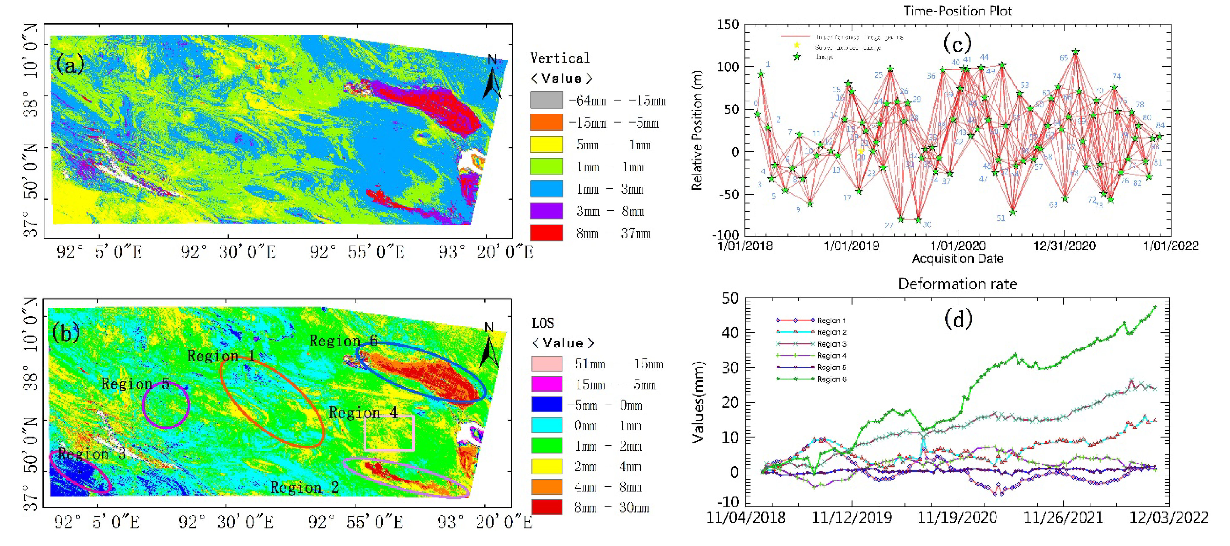
Between 2018 and 2022, we selected a total of 87 descending Sentinel-1A images. The SBAS-InSAR technique was employed to investigate the LOS displacement and vertical displacement characteristics within the study area. After estimating deformation rates and residual topography, the corrected and unwrapped phases were merged and transformed into elevation data. This data was then geocoded under the WGS84 coordinate system, with the LOS deformation values subsequently being converted to vertical deformation values [61]. The outcomes reveal the time-series deformation rates and quantities for the Line-of-Sight (LOS) (Figure 3c) and vertical directions (Figure 3a), as well as the deformation quantities in Figure 3d. An analysis of Figure 3a, and 3b indicates that the overall deformation in the study area fluctuates between -5mm and 4mm. This deformation exhibits a predominantly stable trend, with significant variations in localized regions [62,63,64].
Upon further scrutiny of six sub-regions, deformation quantities for Region1 through Region6 were discerned to range from -6 to 2 mm, 0 to 12 mm, -5 to 22 mm, -1 to 4 mm, -1 to 1 mm, and 0 to 45 mm, respectively. Analyzing these in conjunction with on-site topography and high-resolution optical remote sensing images (Figure S1) revealed that Regions 2 and 6, characterized as lakes and marshlands, exhibited pronounced deformations. Conversely, Regions 3 and 4, identified as dune clusters, exhibited noticeable deformation changes. Regions 1 and 5 encapsulate the overarching environmental conditions of the study area, demonstrating a relatively stable deformation trend, as illustrated in Figure 9a1- a4. Surface horizontal deformation displacement for the periods 2020-2021, 2021-2022, and 2020-2022 was obtained using the COSI-Corr software, as shown in Figure S1.
Figure 3.
ADS80 flight image data acquisition. (a), and (b) Illustrate the vertical and LOS deformation rates. (b) The ellipses colored in red, gray, magenta, pink, purple, and blue each signify six distinct micro-regions representing varying terrain deformation patterns. (c) The red lines delineate interferometric image pairs, while the yellow pentagram marks the master image and the green pentagrams represent respective temporal Sentinel-1A images. (d) Showcases six unique curves that correspond to the deformation changes in the six regions depicted in (b).
By comprehensively analyzing the displacements in LOS, vertical, and horizontal directions (Figure S1) obtained from the integration of InSAR and high-resolution optical remote sensing imagery, it can be inferred that, although multiple faults are distributed within the study area and there have been earthquakes of magnitude less than 5.0MW, the displacements in LOS, vertical, and horizontal directions have been relatively small in recent years. This suggests a relatively stable geological plate and fault activity in the region [37]. Moreover, the predominant landforms in the area consist of plains and small hills, with no extensive high mountains or canyons. These conditions collectively contribute to the favorable enhancement of precision for the subsequent refinement of the quasi-geoid surface using the GNSS gravity-potential leveling model, as detailed in the following sections.
3.2. Accuracy Control in the Acquisition Process of ADS80 Stereo Images
We utilized the KingAir350 aircraft (Figure 4a), equipped with the Leica ADS80 three-line scanner digital photogrammetry aerial survey system (Figure 4a1- a3) to conduct aerial surveys. This allowed us to acquire stereo imagery data with a resolution exceeding 0.2 m for the study area (Figure 4a4). In order to integrate the Leica ADS80 aerial survey system, modifications were made to the KingAir350 aircraft’s payload platform. The resulting configuration, as illustrated in (Figure 4a3), endowed the Kingair350 with the capability to operate in high-altitude plateau environments, with a flight ceiling ranging from 0 to 10,000 m. This ensured compliance with the altitude requirements specified in our flight plan. Using the Mission-Pro flight planning software, a total of 16 east-west flight paths were designed for the study area Figure 4b. The average ground projection spacing between images was 5 km, with an average lateral overlap of 35% between adjacent flight strips. Each flight strip was defined by three waypoints, with the initial and final waypoints serving as the starting and ending points for image capture (Figure 4b). Additionally, a pre-imaging waypoint was established 3 km before the starting point. Upon reaching this waypoint, the gyro-stabilized platform PAV 80, the POS system (IMU + GNSS), and the camera control system CU80 initiated initialization and entered a pre-imaging state. The aerial surveyor used the OI40 monitor to engage in real-time communication with the pilot, discussing the current flight altitude, discrepancies from the designated flight altitude, and aircraft orientation. This facilitated adjustments to the flight path in preparation for a seamless transition into the image capture starting point [65].
Figure 4.
ADS80 Flight Image Data Acquisition. (a) Represents the hardware platform for acquiring stereo imagery in this study. Subfigures include (a1) the KingAir 350 aircraft platform, (a2) the ADS80 digital photogrammetric hardware system, (a3) the installation environment for ADS80 aerial photography, and (a4) the airborne operational status. (b) The blue line indicates the designated flight path, while the pink and yellow filled rectangles denote the distribution of pre-progressive waypoints and cruise starting waypoints, respectively. The purple filled rectangle represents the distribution of Cruise ending waypoints, and the cyan area represents the footprint of single flight line imagery coverage. (c) The red and blue lines represent the actual flight paths of the first and second missions, respectively. The yellow ellipse indicates the Figure-eight flight path before starting the mission, and the cyan rhombus represents the Figure-eight flight path after completing the mission. (d) The red line depicts the designated flight path, and the green triangles represent designated ground control points. (e) The red and blue lines depict the actual flight paths of the first and second missions, respectively. The yellow circular triangles denote Continuously Operating Reference Station (CORS) sites, and the yellow circular filled areas indicate the signal coverage range of CORS sites.
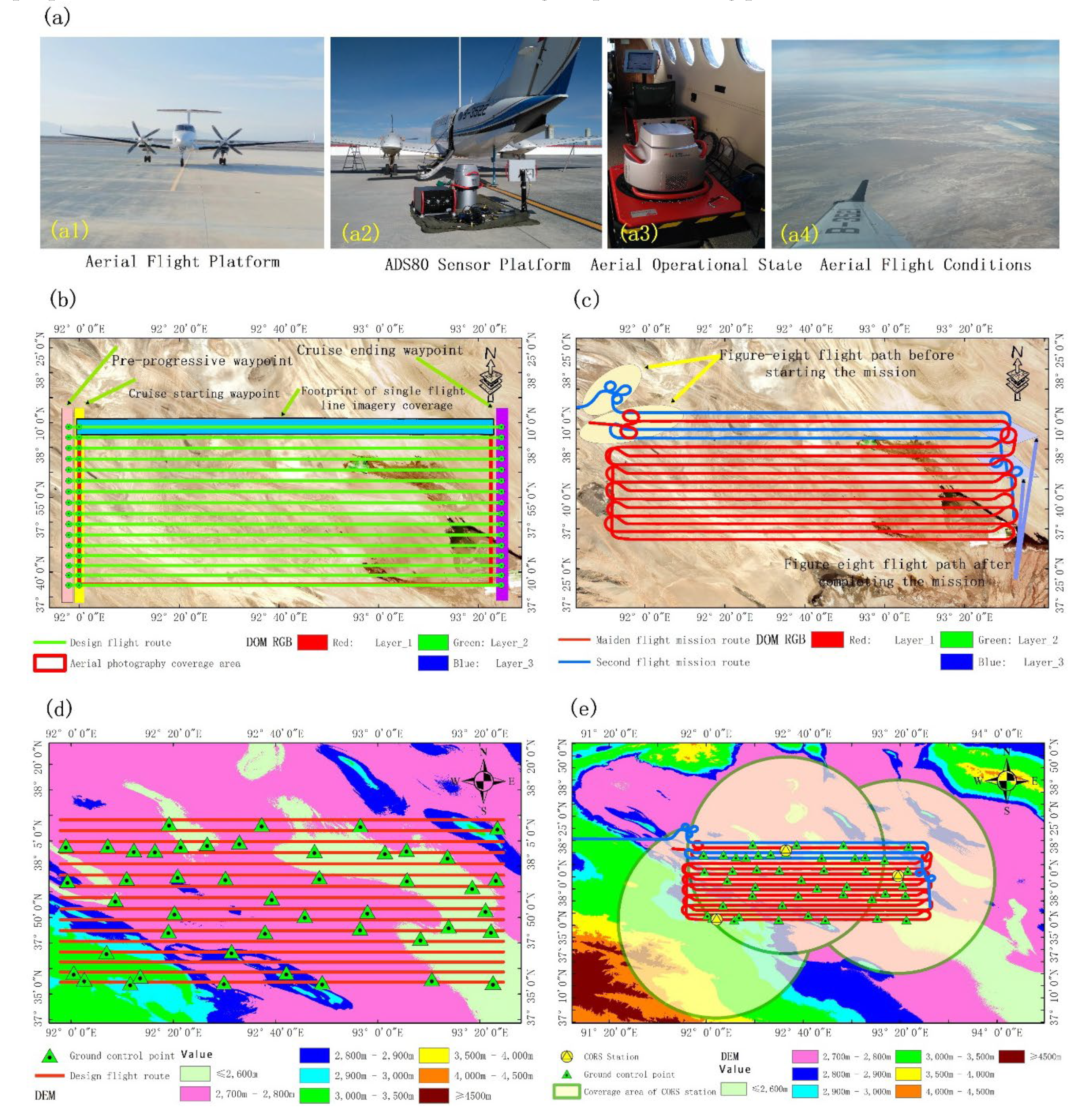
During the aerial survey flights, the aircraft executed a ‘Figure-eight’ flight pattern before reaching the initial waypoint and again after completing the final waypoint. This maneuver was employed to mitigate potential linear drift errors in the IMU resulting from extended flight durations. Additionally, each individual flight path was limited to approximately 30 minutes. T The acquisition of stereo imagery data in the study area was contingent on weather conditions and airspace availability, necessitating two flight missions, as shown in Figure 4c. Prior to the flights, ground control points were established and marked for measurement. The study area adopted a grid-based layout for the distribution of 46 ground control points, as shown in Figure 4d. Given the challenging and high-altitude terrain of the measurement area, we utilized the Precise Point Positioning (PPP) method for ground control point measurements. The Gamit/Globk software, in conjunction with International GNSS Service (IGS) reference stations, was employed for precise coordinate calculations, with all measurements referenced to the CGCS2000 coordinate system [21]. To achieve high-precision POS data, a post-processing differential mode was employed for POS data computation. In the study area, three GNSS reference stations were established, ensuring that the baselines of the GNSS reference stations were confined within a 50 km radius. This setup guaranteed that synchronized observations covered the entirety of the region, as shown in Figure 4e. During the flight of the Leica ADS80 aerial survey system, these stations were activated synchronously, working collaboratively with the onboard differential GNSS receiver. This synchronous observation aimed to counteract errors from factors such as ionospheric and tropospheric disturbances during the computation of onboard differential POS data.
3.3. High-Precision POS Data Post-Differential Processing Accuracy Analysis
After the completion of two flight missions, a Post-Processing Kinematic (PPK) approach was employed [65,66,67] to differentially process the synchronized observations from the GNSS reference stations [67,68] with the acquired POS data. The IE software was used to perform both forward and reverse recursive Kalman filtering fusion (Figure S2) for all exterior orientation elements, including the IMU parameters (roll φ, pitch Ω, and yaw κ) and the GNSS coordinates (X, Y, Z). The GNSS reference station data was sampled at 1 second intervals, while the IMU was sampled at 200 Hz. The processing epochs ranged from 196000 to 212000, as shown in Figure 5a. Observations from four types of satellites, namely GPS, GLONASS, BeiDou, and Galileo, were collected. The Double Difference Dilution of Precision (DD_DOP) values for all observation epochs were between 0.8 and 1.8 (Figure 5b). The partial satellite observation residuals, as listed in Figure 5c, were within the range of -0.04 m to 0.04 m, indicating good and continuous dynamic observations of the satellites during the flight without significant cycle slips or data gaps. This ensured high data quality. Furthermore, an analysis of the PAV80 three-axis stabilized platform’s performance during flight revealed timely corrections made to the roll and pitch angles. The aircraft’s attitude angles were between -30° and 25° during the turn when switching flight lines. After the correction, the roll and pitch angles were within the range of -3° to 3° (Figure S3). Upon transition to the East (E), North (N), and Up (U) directions, the residuals in the E and N directions fluctuated between 0.04 and 0.06 meters, while in the U direction, the residuals varied between 0.1 and 0.26 meters, as shown in Figure 5h. The evident corrective effect demonstrated that the PAV80 three-axis stabilized platform effectively compensated for the instability in the aircraft’s attitude caused by external wind direction and airflow during flight, providing solid support for obtaining high-precision IMU data (Figure 5d).
Figure 5e decomposes the aircraft’s velocity during flight into horizontal (X, Y) and vertical (Z) components. In the X and Z directions, velocity fluctuations are observed around 0 m/s, while in the Y direction, representing the aircraft’s forward motion, the velocity component remains between 110 m/s and 125 m/s. After transformation to E, N, and U coordinates, the residuals fluctuate between 0.12 cm/s and 0.16 cm/s (Figure 5i). Additionally, the aircraft’s flight altitude consistently remains between 7420 m and 7445 m, closely matching the originally designed altitude of 7430 m (Figure 5f), with a deviation of approximately 25 m. These observations affirm that the aircraft maintains high precision in both speed and altitude throughout the flight, providing assurance for the accurate acquisition of stereo imagery. Upon transforming the horizontal (X, Y) and vertical (Z) components into E, N, and U directions, we conducted an analysis of the integrated POS accuracy from IMU (φ, Ω, κ) and GNSS (X, Y, Z) data fusion [38,68]. We found that the fusion error in the E direction fluctuates between -0.1 m and 0.04 m, in the N direction it ranges from -0.06 m to 0.06 m, and in the U direction, it fluctuates between -0.26 m and 0.45 m. All of these errors were found to be below the empirical threshold of 0.5 m, as shown in Figure 5g. For the first and second flights, a total of 312,353 (Figure S4) and 72,116 (Figure S5) POS coordinate data points were calculated, respectively. The aforementioned high-precision POS data provides robust support for subsequent aerial triangulation densification, stereo image model reconstruction, and the collection of three-dimensional coordinates as detailed in the following sections.
3.4. Airborne Triangulation Accuracy Enhancement Analysis
3.4.1. Analysis of Ground Control Point Layout Schemes
To integrate the high-precision POS data calculated in Section 3.3 for aerotriangulation refinement and the establishment of stereoscopic imagery models of the study area, a uniform GCP layout scheme, as described in Section 3.2, was employed across the survey region. A total of 46 GCPs were deployed, with the baseline distance between adjacent control points maintained within 50 km, as shown in Figure 6a, 6g–i depict the challenging environments within the study area where GCP deployment and measurements were conducted. Upon completion of the measurements, all GCPs were processed to the CGCS2000 coordinate system using the Gamit/Globk software, in conjunction with IGS station data, employing the un-differenced ionosphere-free model for PPP [68,69], achieving centimeter-level precision for all resolved GCPs. Leveraging the coordinates of these GCPs, aerotriangulation refinement was performed on the XPro photogrammetric workstation to establish a three-dimensional stereoscopic imagery model of the study area.
To evaluate the impact of different GCP layout schemes on the precision of aerotriangulation refinement, and to select the most optimal and cost-effective layout, the 46 GCPs were categorized into five distinct schemes. Scheme one (Figure 6b) involved using the POS data alone for network adjustment, treating all 46 GCPs as check points to assess the adjustment accuracy. Scheme two (Figure 6c) utilized eight GCPs, with the remaining 38 serving as check points. Scheme three (Figure 6d) increased the number of GCPs to 16, with 30 as check points, while Scheme four (Figure 6e) and Scheme five (Figure 6f) incrementally increased the number of GCPs to 31 and 40, respectively, leaving 15 and 6 as check points.
The intent of Scheme Two was to distribute points around the outer perimeter and central region of the study area to control the precision of the aerotriangulation, while Schemes Three to Five progressively added more control points to ascertain whether a greater number of GCPs indeed contributes to enhanced precision in aerotriangulation. The rationale behind selecting these five schemes was to analyze the minimum number of GCPs required for the study area. This approach aimed to minimize fieldwork in uninhabited regions under adverse environmental conditions, ensuring the safety of the survey personnel, while still satisfying the precision requirements for aerotriangulation refinement.
3.4.2. Analysis of Airborne Triangulation Accuracy under Various GCP Layout Schemes
Bulleted lists look like this: Incorporating the GCP deployment strategy discussed in Section 3.4.1, we conducted a beam method regional network adjustment for aerial triangulation densification using the XPro photogrammetric workstation [38]. Following the adjustment, the errors for the control points and checkpoints for the aforementioned deployment schemes were obtained. For the control point errors, we performed coordinate stabbing, which involved transferring the actual measured locations to their corresponding positions on the images, and carried out a combined regional network adjustment for all control points. This process resulted in obtaining the positional Mean Square Error (MSE) for each control point. Regarding checkpoint errors, upon the combined adjustment of the control point regional network, we transferred the coordinates of points not involved in the adjustment to their corresponding positions on the images. Then, we conducted a combined adjustment for all checkpoints to determine their positional MSE [38,41,65].
As illustrated in Figure 7, in Scheme I, control points were not included in the adjustment, resulting in a zero MSE, while checkpoints exhibited a horizontal MSE of 0.189 m and a vertical MSE of 0.123 m (Figure 7a, and 7b, Table S1). In Scheme II, the inclusion of ground control points increased the horizontal MSE for control points and checkpoints to 0.320 m and 0.235 m, respectively, and the vertical MSE to 0.235 m and 0.114 m (Figure 7c, and 7d, Table S2). This initial estimate suggests that the introduction of GCPs in the regional network adjustment may introduce a systematic bias during the rectification of images from the image space coordinate system to the CGCS2000 coordinate system of the control points. In Scheme III, with an increased number of ground control points, the horizontal MSE for control points and checkpoints was further reduced to 0.119 m and 0.184 m, respectively, with vertical MSE values of 0.115 m and 0.106 m. (Figure 7e, and 7f, Table S3). This indicates an enhancement in the precision of aerial triangulation densification with the increasing number of control points. Continuing the increment in Scheme IV, the horizontal MSE for control points and checkpoints was 0.170 m and 0.150 m, respectively, with a vertical MSE of 0.100 m for control points and 0.133 m for checkpoints. (Figure 7g, and 7h, Table S4). The MSE for control points in the horizontal direction slightly increased, while it decreased in the vertical direction.
Conversely, the checkpoints showed a reduction in horizontal MSE but an increase in vertical MSE, suggesting that the continuous increase in the number of control points positively impacted the vertical precision. In Scheme V, both control points and checkpoints attained the lowest MSE in all five schemes with a horizontal MSE of 0.116 m and 0.083 m, respectively, and a vertical MSE of 0.090 m and 0.053 m (Figure 7h, and 7j, Table S5), Achieving centimeter-level precision, the results fully satisfied the requirements for aerial triangulation densification precision of the study area. In conclusion, the precision of Scheme III (Figure 6d) was found to be comparable to that of Scheme V (Figure 6f). However, Scheme III required only half the number of control points, which could significantly reduce both workload and cost if selected for field control point measurement. Nonetheless, considering that the subsequent reconstruction of a stereo model and the acquisition of high-precision GNSS gravity points in the study area required high accuracy, Scheme V was chosen as the final ground control point deployment strategy.
3.4.3. Extraction of GNSS Gravity-Potential Control Points in Dimensional Environments
In Section 3.4.2, the precision of aerial triangulation densification for control point scheme five, as shown in Figure8g, and 8h, achieved centimeter-level accuracy in both horizontal and vertical directions. Leveraging this precision, the Chinese digital photogrammetric mapping system MapMatrix3D was utilized to construct and restore a digital 3D stereoscopic model of the study area. With the support of a stereoscopic graphics card and wearing 3D glasses, we authentically recreated the stereoscopic scene of the study area, as shown in Figure 8a. Through a combination of different stereoscopic image display modes—namely Pattern 1 (Dual Stereoscopic), Pattern 2 (Anaglyphic), and Pattern 3 (Polarized Light)—and manual interpretation, a total of 594 points coordinates based on the CGCS2000 coordinate system were extracted (pertaining to GNSS gravity-potential control points) within the stereoscopic environment. To control the precision effectively during point extraction, the point positions in the study area were referenced to the decimeter-precision regional quasi-geoid model (Li 2012) of Qinghai province (Qinghai Province Quasi-Geoid Model, QPQM) as depicted in Figure2. Point coordinates were collected near the QPQM model grid points, with an average grid spacing of 2′30” (Figure 8b).
The QPQM model was constructed using 213,862 terrestrial gravity data points within the Qinghai province territory and 101 high-precision GPS leveling data points. The EGM96 was employed as the reference gravity field, with terrain corrections applied using Shuttle Radar Topography Mission (SRTM-3) data. Geoid undulations interpolated and extrapolated via the remove-restore technique incorporating Molodensky’s method. The resultant quasi-geoid of Qinghai province, with a resolution of 2′30” and an accuracy better than 0.186 m [42], was determined by removing the vertical deflections between GPS leveling and the gravity quasi-geoid [43,70]. This model also serves as the foundational grid digital model for refining the regional quasi-geoid using the GNSS gravimetric leveling method in subsequent sections, and it provides a benchmark for precision assessment.
3.5. Airborne Triangulation Accuracy Enhancement Analysis
To evaluate and verify the precision of the GNSS Gravity-Potential Leveling proposed in this study, level measurements were carried out in the study area. Two leveling routes were established and measured as shown in Figure 9a. The first leveling route was located in the southwest of the study area, where six leveling points were measured using a second-order leveling standard. The second route, located in the northeast, traversing the entire study area, and it consisted of 22 leveling points measured at the same second-order leveling standard. Upon completion of the leveling measurement, PPP was employed at the same leveling points to conduct geodetic coordinate measurements (Figure 9a1-a4), using the data processing model proposed in Section 2.4. This resulted in two sets of elevation coordinates for the same leveling points [70,71,72]. The first set based on the 1985 elevation datum normal height coordinate system, and the second set based on the CGCS2000 national elevation datum geoidal height coordinate system.
Figure 9.
This is a figure. Accuracy Analysis of Five Aerial Triangulation Augmentation Schemes. (a) The black lines represent the two leveling routes surveyed in the study area, with the leveling points denoted by yellow circles. The red lines indicate the designed flight paths, while the pale yellow ellipses mark the representative leveling point locations. Subfigures (a1)–(a4) illustrate GNSS measurements taken simultaneously at leveling points across different geographic environments. (b)-(m) represent the Root Mean Square Error (RMSE) values of leveling points computed using twelve geopotential models, namely EGM2008, SGG-UGM-2, SGG-UGM-1, Eigen6C4, GECO, XGM2019e-2159, EGM96, GGM05C, GO-CONS-GCF-2-DIR-R6, Tongji-GMMG2021S, EigenCG03C, and Tongji-GRACE02, respectively.
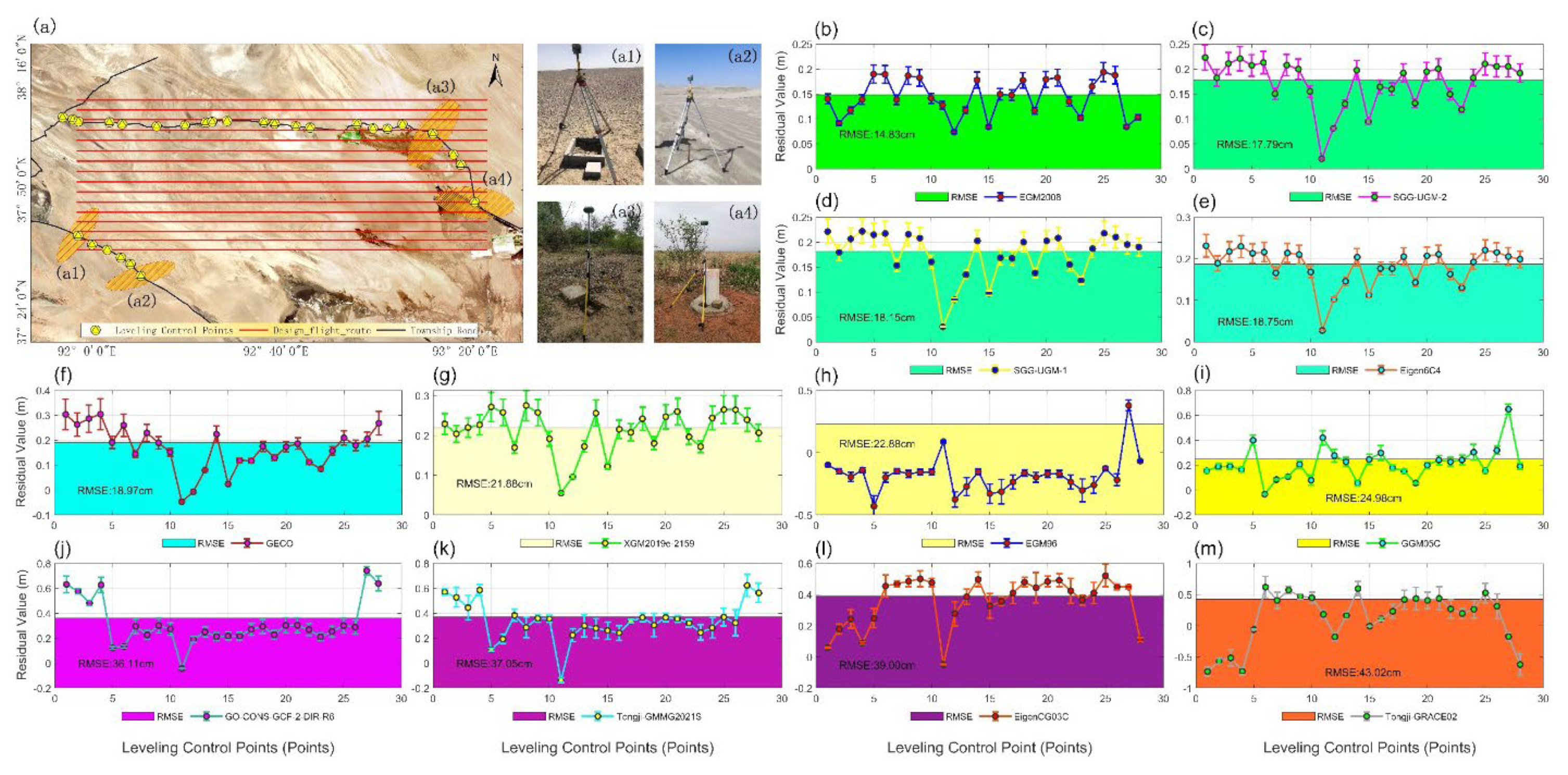
In the application of the GNSS gravity-potential Leveling delineated in Section 2.5, gravity potential values of 593 GNSS points extracted in a stereo environment compared with the average normal gravity value (Figure S6-S17). These calculated normal heights were then subjected to an RMS accuracy analysis against the measured normal heights, as per the methodologies discussed by [72]. Prior to this, the gravity potential values at the leveling points were computed using the gravity potential model described in Section 2.5.2 (Figure S18, and S19). The geopotential value at the elevation reference point, specifically the sea-level datum at the Qingdao tide gauge, as shown in Figure 1, was set at 62,636,854.205 m2/s2, in accordance with [56,70] Further, the mean gravity values at each leveling point were calculated using the average normal gravity model outlined in Section 2.5.3. To analyze the impact of various satellite gravity models on the precision of normal height calculations for leveling points in the study area, we selected twelve different satellite gravity models. The spherical harmonic coefficients of the five models (EGM2008, SGG-UGM-1, SGG-UGM-2, Eigen-6C4, GECO) were extended up to degree and order 2159, as supported by the works of Liang et al. [13], Zingerle et al. [14], Gilardoni et al. [15], and Chisenga et al. [16].
Figure 9 illustrates the residual values for leveling points computed by each satellite gravity mission. Notably, the EGM2008 satellite gravity model yielded the lowest RMSE value of 14.83 cm, as shown in Figure 9b, followed by the SGG-UGM-2 and SGG-UGM-1 models with RMSE values of 17.79 cm and 18.15 cm, respectively, as shown in Figure 9c, and 9d. Models with an RMSE value below 20 cm included Eigen6C4 and GECO, registering values of 18.75 cm and 18.97 cm, as shown in Figure 9e, and 9f. The models XGM2019e-2159, EGM96, and GGM05C had RMSE values of 21.88 cm, 22.88 cm, and 24.96 cm, respectively, as shown in Figure 9g- i. The GO-CONS-GCF-2-DIR-R6, Tongji-GMMG2021S, and EigenCG03C models exhibited larger RMSEs of 36.11 cm, 37.05 cm, and 39.00 cm, respectively (Figure 9j-l). A preliminary estimate indicates that the lower accuracy of these models may be attributed to their relatively lower degree of spherical harmonic expansion. The Tongji-GRACE02 model showed the largest RMSE of 43.02 cm (Figure 9m), due to its harmonic coefficients being expanded only to the 180th degree, the lowest among the models analyzed.
3.6. Airborne Triangulation Accuracy Enhancement Analysis
As concluded in Section 3.5, the normal heights computed using the GNSS gravitational geopotential height leveling in this study exhibit superior RMSE precision over the QPQM regional geoid model (18.6 cm). This is particularly evident with the EGM2008 (14.83 cm), SGG-UGM-2 (17.79 cm), and SGG-UGM-1 (18.15 cm) satellite gravity models, as shown in Figure 9b-d. This finding validates the feasibility of the GNSS leveling method proposed in this paper, which is grounded on the actual precision of the leveling points. Utilizing the theoretical model of GNSS gravitational geopotential height leveling as described in Section 2.5.1, this study calculates the normal heights for all 594 points (pertaining to GNSS gravity-potential control points) collected under the three-dimensional models outlined in Section 3.4.3, based on the CGCS2000. To enhance the accuracy of the GNSS leveling method, a grid error correction approach is employed [7,33,56], wherein the normal heights obtained from leveling measurements, H_1985, are used to correct the normal heights derived from the GNSS leveling models, H_GNSS.
After Correction, we calculated the residuals of the normal height (H_GNSS) and the RMSE values for the three-dimensional solid model collected GNSS points, using twelve gravity satellite models. Post-correction, both the residuals (Figure 10a) and the precision of RMSE values exhibited significant improvements. The EGM2008 gravity satellite model showed the minimum residuals and RMSE values (Figure 10b), which were 6.90 cm and 8.61 cm, respectively. Subsequently, the SGG-UGM-2 and SGG-UGM-1 gravity satellite models presented residuals and RMSE values of -8.10 cm, -7.70 cm, 9.09 cm, and 9.38 cm respectively, as shown in Figure 10a, and 10d. Gravity satellite models with residuals in the -20 cm to 20 cm range included Eigen6C4 and GECO, while those with RMSE values in the 10 cm to 20 cm range comprised Eigen6C4, GECO, and XGM2019e-2159, as shown in Figure 10e, and 10f. The EGM96 and GGM05C models yielded residuals and RMSE values of 16.70 cm, -22.30 cm, 23.74 cm, and 25.59 cm respectively, as shown in Figure 10h, and 10i. The models G0-CONS-GCF-2-DIR-R6, Tongji-GMMG2021S, and EigenCG03C recorded residuals and RMSE values of -14.60 cm, -15.70 cm, -38.20 cm, 29.98 cm, 36.18 cm, and 39.91 cm respectively, as shown in Figure 10, and 10l. Lastly, the Tongji-GARCE02 gravity satellite model had residuals and RMSE values of 42.90 cm and 43.02 cm, respectively (Figure 10m).
Accordingly, it can be deduced that the EGM2008, SGG-UGM-2, and SGG-UGM-1 gravity satellite models, after refinement with level data corrections, achieve centimeter-level accuracy, which is superior to the original regional quasi-geoid model, QPQM. This demonstrates the feasibility and significant improvement in precision of the methodology proposed in this paper. The methodology employs the ADS80 tri-linear array pushbroom stereo imaging for aerial triangulation enhancement in conjunction with GNSS gravimetric geoid model data fusion for further refinement of the quasi-geoid in the study area. Furthermore, based on precision requirements, other gravity satellite models can be selectively utilized to establish a regional quasi-geoid surface. For example, when the accuracy requirement is between 10 cm and 20 cm, the Eigen6C4, GECO, and XGM2019e-2159 models are suitable candidates. For precision between 20 cm and 30 cm, the EGM96, GGM05C, and G0-CONS-GCF-2-DIR-R6 models may be adopted. In the range of 30 cm to 40 cm accuracy, the Tongji-GMMG2021S and EigenCG03C models could be selected. Lastly, for accuracy demands above 40 cm, the Tongji-GRACE02 gravity satellite model would be appropriate.
4. Discussion
4.1. Influence of Different Gravity Field Models on the Accuracy of Regional Quasi-Geoid
The method proposed in this article, which utilizes the ADS80 three-line array pushbroom stereo imaging aerial triangulation technique integrated with GNSS geopotential level model data processing for orthometric height computation, to a certain extent, it can replace traditional leveling measurements, and it facilitates the rapid restoration and establishment of regional quasigeoid surfaces. It can be inferred from Table S6 that the higher the degree of spherical harmonic expansion in the adopted gravity satellite model (ranging from degrees 180 to 2190), the higher the accuracy of the solution provided by the GNSS geopotential leveling method [17,19,21]. An accuracy analysis using leveling data measured on-site within our study area revealed that the precision of the orthometric heights computed by this method surpasses that of the existing QPQM quasi-geoid surface. Moreover, after the correction of leveling data, the accuracy of GNSS points collected via the stereo model based on the EGM2008, SGG-UGM-2, and SGG-UGM-1 gravity satellite models can achieve centimeter-level precision. Enables the rapid computation and restoration of the 1985 orthometric height datum in the study region. This is achieved without relying on ground leveling or terrestrial gravity data [19,22,71]. This is particularly crucial for providing high-accuracy regional quasi-geoid models in the uninhabited, high-altitude areas of the Tibetan Plateau, thereby offering robust theoretical and precision support.
4.2. Impact of Various Errors on GNSS Gravity-Potential Leveling
The GNSS Gravity-Potential Leveling discussed in this article is subject to various errors during the computation process [18,70]. In particular, the King Air 350 aircraft, equipped with an ADS80 photogrammetric camera, incurs flight errors due to multiple flight factors, including wind speed, wind direction, air currents, and flight attitude, especially when navigating a “figure-eight” trajectory as described in Section 3.2 Errors also arise from the measurement of GCPs and the processing inaccuracies within the Gamit/Globk software, as well as from the discrepancies in post-processing differential PPK POS data calculation (as set out in Section 3.3, with a 50 km baseline among three neighboring GNSS reference stations). Errors associated with POS-assisted aerial triangulation densification and pinpointing (various control point deployment strategies are detailed in Section 3.4.1), the reconstruction of three-dimensional stereo model point collection (three modes of stereo image display are analyzed in Section 3.4.3), and GNSS geopotential leveling resolution errors (including zero-order and tidal terms) are further considered. A detailed accuracy analysis concerning these various errors is conducted to ensure that the precision of the original data can substantiate and bolster the computational accuracy of the GNSS geopotential leveling method proposed herein [71,72]. As the accuracy of flight platforms, photogrammetric cameras, GNSS satellites, and gravity satellite hardware platforms improves, along with the stabilization and refinement of modeling and computational approaches, a reduction in the aforementioned errors is anticipated. This reduction is expected to provide even more favorable assurance for enhancing the precision of the GNSS geopotential leveling method elaborated in this paper.
4.3. Characteristics of Refined Regional Quasi-Geoid Models
Upon refining the normal heights calculated by the GNSS gravimetric geoid determination method using leveling data, we derived the regional elevation anomaly values (Figure 1). Subsequently, these ξ values facilitated the reconstruction of the quasi-geoid model within our study area, as shown in Figure 11. It is evident that the surface of elevation anomalies modeled by QPQM, as shown in Figure 11a, is consistent with the surface derived from the GNSS gravimetric geoid method using gravity satellite data, as seen in Figure 11a1, and a12, this consistency is observed both in terms of trend distribution and magnitude. They exhibit a pattern where the eastern region is lower and the western region higher, with elevation anomalies ranging between -60 m and 54 m, indicating minimal variation. This aligns with the conclusion in Section 3.1 that our study area is dominated by desolate, arid ‘yardang’ landforms. It is sparsely populated and relatively flat, with stable LOS and vertical ground deformation trends over time, and minimal fault-related horizontal displacements.
The quasi-geoid model within the research area, recovered using values, underwent the extraction and analysis of residual values (Figure 12). It was observed that the interval of residual values for elevation anomalies falls within the range of -0.556m to -0.595m. For the three gravity satellite models, EGM2008, SGG-UGM-2, and SGG-UGM-1, the residuals of the computed elevation anomalies lie between -0.102m and 0.104m. These are lower than those derived from other gravity satellite models, according to their respective accuracies, as discussed in Section 3.6. This further underscores that, for the study area in this paper, utilizing the GNSS gravity-potential leveling to analyze the regional refinement precision enhancement effect of the quasi-geoid, EGM2008, SGG-UGM-2, and SGG-UGM-1 are the optimal choices among the three gravity satellite models. Other gravity satellite models can be selectively chosen based on varying precision requirements.
As our focus is on the normal height system under the 1985 elevation datum of China, an analysis of the ξ values was conducted. However, the analysis revealed that the GNSS gravimetric geoid model proposed in this paper is equally applicable to the calculation of orthometric heights within the WGS84 global elevation datum framework [7,57]. The Quasi-geoid undulation, denoted as , and the gravitational potential of the WGS84 geoid, (62636856.00±0.5 m2/s2), along with the mean gravity, [7,58,59,60], can be calculated using the aforementioned twelve satellite gravity models. This facilitates the establishment of a transformation relationship with the global elevation datum.
5. Conclusions
In our study area situated in the unmanned, high-altitude region of the Tibetan Plateau, we have conducted an accuracy analysis of stereoscopic imagery acquisition and aerial triangulation densification using the ADS80 aerial camera. This analysis was coupled with empirical data from 26 leveling points and 12 GNSS gravity-potential models to synthesize and analyze the feasibility and accuracy improvement effects of this method in refining the regional quasi-geoid. It was found that among these gravity-potential models, including EGM2008, SGG-UGM-1, EIGEN-6C4, and GECO, the models were able to achieve decimeter-level RMSE in the orthometric heights. These heights were derived from the 593 GNSS points collected on the stereoscopic image model after aerial triangulation densification, with respect to the China 1985 Yellow Sea Datum and the leveling point heights. Specifically, the EGM2008, SGG-UGM-2, and SGG-UGM-1 gravity-potential models displayed the highest precision, with RMSEs of 14.83 cm, 17.79 cm, and 18.15 cm, respectively, which are comparable to the precision of the QPQM model.
Upon comprehensive analysis, it has been determined that for regional quasi-geoid refinement without correction through leveling data, the following gravimetric models can be selected based on the desired accuracy levels: For precision requirements between 10 cm and 20 cm, the Eigen-6C4, GECO, and XGM2019e-2159 models are suitable; for a precision range of 20 cm to 30 cm, the EGM96, GGM05C, and GO-CONS-GCF-2-DIR-R6 models can be employed; for precision between 30 cm and 40 cm, the Tongji-GMMG2021S and Eigen-CG03C models are recommended; and for accuracies exceeding 40 cm, the Tongji-GRACE02 model is advisable. After the leveling data are corrected using the weighted average method, the computed 1985 elevation accuracy of each gravimetric model significantly improves, with the EGM2008, SGG-UGM-2, and SGG-UGM-1 models achieving precisions of 8.61 cm, 9.09 cm, and 9.38 cm, respectively, all surpassing the precision of the QPQM model. The enhancements range from 9.22 cm to 9.99 cm in magnitude, indicating that the methods proposed in this paper can significantly improve the accuracy of the regional quasi-geoid. This also provides a new approach for the rapid establishment of regional quasi-geoid models in the unmanned areas of the Tibetan Plateau.
Supplementary Materials
The following supporting information can be downloaded at: https://zenodo.org/records/12567210; Figure S1 to Figure S1, Table S1 to Table S6.
Author Contributions
Conceptualization, W.X., G.C., K.D., X.M. and S.Z.; Data curation, W.X., G.C., K.D., X.M. and Y.Z.; Formal analysis, W.X., D.Y., R.D., S.Z. and Y.Z.; Funding acquisition, G.C. and K.D.; Methodology, W.X., D.Y., R.D. and Y.Z.; Project administration, S.H.; Resources, S.H.; Software, W.X., D.Y. and S.Z.; Supervision, R.D. and S.H.; Visualization, G.C.; Writing—original draft, W.X. and K.D.; Writing—review & editing, W.X.
Funding
This project was funded by the National Natural Science Foundation of China (Grant Nos. 41674015, 42004001, 42274012), the Qinghai high-resolution remote sensing data industrialization application fund project (94-Y40G14-9001-15/18), and the China University of Geosciences (Wuhan) Yangtze River Source Scientific Expedition ‘Three All-Round Education’ Demonstration Project (2022171).
Data Availability Statement
Publicly available datasets were analyzed in this study. They can be found as follows: the Sentinel-1 SAR data were downloaded from the Sentinel-1 Scientific Data Hub https://vertex.daac.asf.alaska.edu. GF series satellite data were derived from the high-resolution Earth observation system of the Qinghai Provincial Remote Sensing Center for Natural Resources, available at https://www.qhgfrs.cn/publiccms. Figures were made with Correlation (COSI-Corr) software (Türk et al. 2018). All the satellite gravity model were sourced from the International Centre for Global Earth Models (ICGEM) at https://icgem.gfz-potsdam.de.
Acknowledgments
We are grateful to the anonymous reviewers for their constructive comments and suggestions to improve this manuscript.
Conflicts of Interest
The authors declare no competing interests.
References
- Molodenskiĭ, M.S.; Еремеев, В.Ф.; Yurkina, M.I. Methods for study of the external gravitational field and figure of the earth. 1962.
- Stokes, G.G. On the Variation of Gravity at the Surface of the Earth. In Cambridge University Press eBooks. 2010, pp. 131–171.
- Sjöberg, L.E. On the existence of solutions for the method of Bjerhammar in the continuous case. Bull. Geod. 1979b, 53, 227–230. [Google Scholar] [CrossRef]
- Erol, S.; Erol, B. A. Comparative assessment of different interpolation algorithms for prediction of GNSS/levelling geoid surface using scattered control data. Measurement. 2021, 173, 108623. [Google Scholar] [CrossRef]
- Ligas, M.; Kulczycki, M. Kriging and moving window kriging on a sphere in geome-tric (GNSS/levelling) geoid modelling. Surv. Revi. 2016, 50, 155–162. [Google Scholar] [CrossRef]
- Wu, Y.; Zhou, H.; Zhong, B.; Luo, Z. Regional gravity field recovery using the GOCE gravity gradient tensor and heterogeneous gravimetry and altimetry data. J. Geophys. Res. Solid Earth. 2017, 122, 6928–6952. [Google Scholar] [CrossRef]
- Wei, Z. Q. GPS gravity-potential Leveling. J. Geod. Geodyn. 2007, 27, 1–7. [Google Scholar]
- Brown, N.J.; McCubbine, J.; Featherstone, W.; Gowans, N.; Woods, A.; Baran, I. AUSGeoid2020 combined gravimetric–geometric model: location-specific uncertainties and baseline-length-dependent error decorrelation. J. Geod. 2018, 92, 1457–1465. [Google Scholar] [CrossRef]
- Boesch, R.; Bühler, Y.; Marty, M.; Ginzler, C. Comparison of digital surface models for snow depth mapping with UAV and aerial cameras. Int. Arch. Photogramm. Remote Sens. Spat. Inf. Sci. 2016, XLI-B8, 453–458.
- Müller, J.; Gärtner-Roer, I.; Thee, P.; Ginzler, C. Accuracy assessment of airborne photogrammetrically derived high-resolution digital elevation models in a high mountain environment. ISPRS J. Photogramm. Remote Sens. 2014, 98, 58–69. [Google Scholar] [CrossRef]
- Klees, R.; Slobbe, D.C.; Farahani, H. A methodology for least-squares local quasi-geoid modelling using a noisy satellite-only gravity field model. J. Geod. 2017, 92, 431–442. [Google Scholar] [CrossRef]
- Farahani, H.H.; Slobbe, D. C.; Klees, R.; Seitz, K. Impact of accounting for coloured noise in radar altimetry data on a regional quasi-geoid model. J. Geod. 2017, 91:97–112.
- Liang, W.; Li, J.; Xu, X.; Zhang, S.; Zhao, Y. A High-Resolution Earth’s Gravity Field Model SGG-UGM-2 from GOCE, GRACE, Satellite Altimetry, and EGM2008. Engineering. 2020b, 6, 860–878. [Google Scholar] [CrossRef]
- Zingerle, P.; Pail, R.; Gruber, T.; Oikonomidou, X. The combined global gravity field model XGM2019e. J. Geod. 2020, 94. [Google Scholar] [CrossRef]
- Gilardoni, M.; Reguzzoni, M.; Sampietro, D. GECO: a global gravity model by locally combining GOCE data and EGM2008. Studia Geophys. et Geod. 2016, 60, 228–247. [Google Scholar] [CrossRef]
- Chisenga, C.; Yan, J. A new crustal thickness model for mainland China derived from EIGEN-6C4 gravity data. J. Asian Earth Sci. 2019, 179, 430–442. [Google Scholar] [CrossRef]
- Pavlis, N.K.; Holmes, S.A.; Kenyon, S. The development and evaluation of the Earth Gravitational Model 2008 (EGM2008). J. Geophys. Res. Solid Earth. 2012, 117. [Google Scholar] [CrossRef]
- Klees, R.; Slobbe, D.C.; Farahani, H. How to deal with the high condition number of the noise covariance matrix of gravity field functionals synthesised from a satellite-only global gravity field model? J. Geod. 2018, 93, 29–44. [Google Scholar] [CrossRef]
- Li, H.P.; Bian, S.F.; Li, Z.M. Chinese Geodetic Coordinate System 2000 and its Comparison with WGS84. Appl. Mech. Mater. 2014, 580–583, 2793–2796.
- Cheng, P.; Cheng, Y.; Wang, X.; Xu, Y. Update China geodetic coordinate frame considering plate motion. Satell. Navig. 2021, 2. [Google Scholar] [CrossRef]
- Yang, Y. Chinese geodetic coordinate system 2000. Sci. Bull. 2009, 54, 2714–2721. [Google Scholar] [CrossRef]
- Cheng, P.; Cheng, Y.; Wang, X.; Wu, S.; Xu, Y. Realization of an optimal dynamic geodetic reference frame in China: Methodology and applications. Engineering. 2020, 6, 879–897. [Google Scholar] [CrossRef]
- Zhu, Y.; Li, K.; Myint, S.W.; Du, Z.; Li, Y.; Cao, J.; Liu, L.; Wu, Z. Integration of GF-2 optical, GF3 SAR, and UAV data for estimating aboveground biomass of China’s largest artificially planted mangroves. Remote Sens. 2020, 12, 2039. [Google Scholar] [CrossRef]
- Tang, X.; Xie, J.; Liu, R.; Guo, Q, H.; Zhao, C.; Zhen, Y.; Tang, H.; Dou, X. Overview of the GF-7 Laser Altimeter System Mission. Earth Space Sci. 2020, 7 (1).
- Dong, S.; Samsonov, S.; Yin, H.; Ye, S.; Cao, Y. Time-series analysis of subsidence associated with rapid urbanization in Shanghai, China measured with SBAS InSAR method. Environ. Earth. Sci. 2013, 72, 677–691. [Google Scholar] [CrossRef]
- Zhao, R.; Li, Z. W.; Feng, G.; Wang, Q.; Hu, J. Monitoring surface deformation over permafrost with an improved SBAS-InSAR algorithm: With emphasis on climatic factors modeling. Remote Sens. Environ. 2016, 184, 276–287. [Google Scholar] [CrossRef]
- Baird, T.R.; Bristow, C.S.; Vermeesch, P. Measuring Sand Dune Migration Rates with COSI-Corr and Landsat: Opportunities and Challenges. Remote Sens. 2019, 11, 2423. [Google Scholar] [CrossRef]
- Türk, T. Determination of mass movements in slow-motion landslides by the Cosi-Corr method. Geomatics, Nat. Hazards Risk. 2018, 9, 325–336.
- Zhao, F.; Meng, X.; Zhang, Y.; Chen, G.; Su, X.; Yue, D. Landslide Susceptibility Mapping of Karakorum Highway Combined with the Application of SBAS-InSAR Technology. Sensors. 2019, 19, 2685. [Google Scholar] [CrossRef] [PubMed]
- Arnedo, J.P.G.; Pérez-Peña, J.V.; Azañón, J.M.; Closson, D.; Calò, F.; Reyes-Carmona, C.; Jabaloy, A.; Ruano, P.; Mateos, R.M.; Notti, D.; Herrera, G.; Béjar-Pizarro, M.; Monserrat, O.; Bally, P. Evaluation of the SBAS INSAR service of the European Space Agency’s Geohazard Exploitation Platform (GEP), Remote Sens. 2017, 9, 1291.
- Wang, H.; Wang, C.; Wu, H. Using GF-2 imagery and the conditional random field model for urban forest cover mapping. Remote Sens. Lett. 2016, 7, 378–387. [Google Scholar] [CrossRef]
- Ren, C.; Xie, J.; Xiong, Z.; Ye, Y.; Yang, S. Laser Spot Center location method for Chinese spaceborne GF-7 footprint camera. Sensors. 2020, 20, 2319. [Google Scholar] [CrossRef] [PubMed]
- Wang, J.; Hu, X.; Meng, Q.; Zhang, L.; Wang, C.; Liu, X.; Zhao, M. Developing a Method to Extract Building 3D Information from GF-7 Data. Remote Sens. 2021, 13(22), 4532. [Google Scholar] [CrossRef]
- Zhang, C.; Cui, Y.; Zhu, Z.; Jiang, S.; Jiang, W. Building Height Extraction from GF-7 Satellite Images Based on Roof Contour Constrained Stereo Matching. Remote Sens. 2022, 14, 1566. [Google Scholar] [CrossRef]
- Hermas, E.; Leprince, S.; El-Magd, I. A. Retrieving sand dune movements using sub-pixel correlation of multi-temporal optical remote sensing imagery, northwest Sinai Peninsula, Egypt. Remote Sens. Environ. 2012, 121, 51–60. [Google Scholar] [CrossRef]
- Scheidt, S. P.; Lancaster, N. The application of COSI-Corr to determine dune system dynamics in the southern Namib Desert using ASTER data. Earth Surf. Process. Landf. 2013, 38, 1004–1019. [Google Scholar] [CrossRef]
- Yao, J.; Yao, X.; Liu, X. Landslide detection and mapping based on SBAS-INSAR and PS-INSAR: a case study in Gongjue County, Tibet, China. Remote Sens. 2022, 14, 4728. [Google Scholar] [CrossRef]
- Hobi, M. L.; Ginzler, C. Accuracy assessment of digital surface models based on WorldView-2 and ADS80 stereo remote sensing data. Sensors. 2012, 12, 6347–6368. [Google Scholar] [CrossRef] [PubMed]
- Grünewald, T.; Bühler, Y.; Lehning, M. Elevation dependency of mountain snow depth. Cryosphere. 2014, 8, 2381–2394. [Google Scholar] [CrossRef]
- Liu, K.; Ding, H.; Tang, G.; Na, J.; Huang, X.; Xue, Z.; Yang, X.; Li, F. Detection of Catchment-Scale Gully-Affected Areas using unmanned aerial vehicle (UAV) on the Chinese Loess Plateau. ISPRS Int. J. Geoinf. 2016, 5, 238. [Google Scholar] [CrossRef]
- Ginzler, C.; Hobi, M.L. Countrywide Stereo-Image matching for updating digital surface models in the framework of the Swiss National Forest Inventory. Remote Sens. 2015, 7, 4343–4370. [Google Scholar] [CrossRef]
- Li, J.; Zhan, W.; Guo, B.; et al. Combination of the Levenberg–Marquardt and differential evolution algorithms for the fitting of postseismic GPS time series. Acta Geophys. 2021, 69, 405–414. [Google Scholar] [CrossRef]
- Klees, R.; Prutkin, I. The combination of GNSS-levelling data and gravimetric (quasi-) geoid heights in the presence of noise. J. Geod. 2010, 84, 731–749. [Google Scholar] [CrossRef]
- Albayrak, M.; Özlüdemir, M.T.; Aref, M.M.; Halıcıoğlu, K. Determination of Istanbul geoid using GNSS/levelling and valley cross levelling data. Geod. Geodyn. 2020, 11, 163–173. [Google Scholar] [CrossRef]
- Li, W.; Cardellach, E.; Fabra, F.; Ribó, S.; Rius, A. Lake level and surface topography measured with spaceborne GNSS-Reflectometry from CYGNSS Mission: example for the Lake Qinghai. Geophys. Res. Lett. 2018, 45. [Google Scholar] [CrossRef]
- Chisenga, C.; Yan, J. A new crustal thickness model for mainland China derived from EIGEN-6C4 gravity data. J. Asian Earth Sci. 179, 430–442. [CrossRef]
- Liu, Y. Analysis of GAMIT/GLOBK in high-precision GNSS data processing for crustal deformation. Earthq. Res. Adv. 2021, 1, 100028. [Google Scholar] [CrossRef]
- Ryanda, K.; Handoko, E. Y.; Maulida, P. Land Subsidence Study using Geodetic GPS and GAMIT/GLOBK software (Case study: Banjarasri Village and Kedungbanteng Village, Tanggulangin District, Sidoarjo Regency). IOP Conf. Ser.: Earth Environ. Sci. 2021, 936, 012020.
- Alçay, S.; Öğütçü, S.; Kalaycı, İ.; Yiğit, C.Ö. Displacement monitoring performance of relative positioning and Precise Point Positioning (PPP) methods using simulation apparatus. Adv. Space Res. 2019, 63, 1697–1707. [Google Scholar] [CrossRef]
- Liang, W.; Xu, X.; Li, J.; Zhu, G. The determination of an ultra-high gravity field model SGG-UGM-1 by combining EGM2008 gravity anomaly and GOCE observation data. Acta Geod. Cartogr. Sin. 2018, 47, 425–434. [Google Scholar]
- Ali, S. H. Technical Report: Determination of the orthometric height inside Mosul University campus by using GPS data and the EGM96 gravity field model. J. Appl. Geod. 2007, 1. [Google Scholar] [CrossRef]
- Milyukov, V.K.; Yeh, H. Next Generation Space Gravimetry: Scientific tasks, concepts, and realization. Astron. Rep. 2018, 62, 1003–1012. [Google Scholar] [CrossRef]
- Rummel, R.; Yi, W.; Stummer, C. GOCE gravitational gradiometry. J. Geod. 2011, 85, 777–790. [Google Scholar] [CrossRef]
- Chen, Q.; Shen, Y.; Francis, O.; Wu, C.; Zhang, X.; Hsu, H. Tongji-Grace02S and Tongji-Grace02K: High-Precision static GRACE-Only global Earth’s gravity field models derived by refined data processing strategies. J. Geophys. Res. Solid Earth. 2018, 123, 6111–6137. [Google Scholar] [CrossRef]
- Erol, B.; Sideris, M. G.; Çeli̇K, R. N. Comparison of global geopotential models from the champ and grace missions for regional geoid modelling in Turkey. Stud. Geophys. Geod. 2009, 53, 419–441. [Google Scholar] [CrossRef]
- Li, J.C.; Chu, Y. H.; Xu, X.Y. Determination of Vertical Datum Offset between the Regional and the Global Height Datum. Acta Geod. Cartogr. Sin. 2017, 46, 1262- 1273.
- Brown, N.J.; Featherstone, W.; Hu, G.; Johnston, G. AUSGeoid09: a more direct and more accurate model for converting ellipsoidal heights to AHD heights. J. Spat. Sci. 2011, 56, 27–37. [Google Scholar] [CrossRef]
- Slobbe, C.; Klees, R.; Farahani, H.H.; Huisman, L.; Alberts, B.; Voet, P.; De Doncker, F. The impact of noise in a GRACE/GOCE global gravity model on a local Quasi-Geoid. J. Geophys. Res. Solid Earth. 2019, 124, 3219–3237. [Google Scholar] [CrossRef]
- Ditmar, P.; Klees, R.; Liu, X. Frequency-dependent data weighting in global gravity field modeling from satellite data contaminated by non-stationary noise. J. Geod. 2006, 81, 81–96. [Google Scholar] [CrossRef]
- Denker, H. Regional Gravity Field modeling: Theory and Practical results. In Springer eBooks. 2012, pp. 185–291).
- Li, S.; Xu, W.; Li, Z. Review of the SBAS InSAR Time-series algorithms, applications, and challenges. Geod. Geodyn. 2022, 13, 114–126. [Google Scholar] [CrossRef]
- Jiang, C.; Fan, W.Y.; Yu, N.; Nan, Y. A new method to predict gully head erosion in the Loess plateau of China based on SBAS-INSAR. Remote Sens. 2021, 13, 421. [Google Scholar] [CrossRef]
- Jin, Z.; Fialko, Y. Coseismic and early postseismic deformation due to the 2021 M7.4 Maduo (China) earthquake. Geophys. Res. Lett. 2021, 48.
- Cigna, F.; Tapete, D. Sentinel-1 Big Data Processing with P-SBAS InSAR in the Geohazards Exploitation Platform: An Experiment on Coastal Land Subsidence and Landslides in Italy. Remote Sens. 2021, 13, 885. [Google Scholar] [CrossRef]
- Bühler, Y.; Marty, M.; Ginzler, C. High resolution DEM generation in High-Alpine terrain using airborne remote sensing techniques. Trans. GIS. 2012, 16, 635–647. [Google Scholar] [CrossRef]
- Heid, T.; Kääb, A. Evaluation of existing image matching methods for deriving glacier surface displacements globally from optical satellite imagery. Remote Sens. Environ. 2012, 118, 339–355. [Google Scholar] [CrossRef]
- Dumka, R.K.; Chopra, S.; Prajapati, S. GPS derived crustal deformation analysis of Kachchh, zone of 2001(M7.7) earthquake, Western India. Quatern. Int. 2019, 507, 295–301.
- Tomaštík, J.; Mokroš, M.; Surový, P.; Grznárová, A.; Merganič, J. UAV RTK/PPK Method—An optimal solution for mapping inaccessible forested Areas? Remote Sens. 2019, 11, 721. [Google Scholar] [CrossRef]
- Çetin, S.; Aydın, C.; Doğan, U. Comparing GPS positioning errors derived from GAMIT/GLOBK and Bernese GNSS software packages: A case study in CORS-TR in Turkey. Surv. Rev. 2018, 51, 533–543. [Google Scholar] [CrossRef]
- Zhang, C.; Dang, Y.; Jiang, T.; Guo, C.; Ke, B.; Wang, B. Heterogeneous gravity data fusion and gravimetric quasigeoid computation in the coastal area of China. Mar. Geod. 2017, 40, 142–159. [Google Scholar] [CrossRef]
- Trojanowicz, M.; Osada, E.; Karsznia, K. Precise local quasigeoid modelling using GNSS/levelling height anomalies and gravity data. Surv. Rev. 2018, 52, 76–83. [Google Scholar] [CrossRef]
- Eshagh, M.; Zoghi, S. Local error calibration of EGM08 geoid using GNSS/levelling data. J. Appl. Geophys. 2016, 130, 209–217. [Google Scholar] [CrossRef]
Figure 1.
GNSS gravity-potential leveling model and the height system. In this figure, all equations and symbols are defined as per Section 2.5, Equations (1)-(10). It includes the Topography Model, Telluroid Model, Geoid Model, and Ellipsoid Model, which are simulation models used to visualize the Ellipsoid (Green), Geoid (Yellow), Telluroid (Blue), and Topography (Red). Flight1 and Flight2 denote the temporal stages of the aircraft flights, illustrating the process of acquiring ADS80 stereo imagery. The flowchart in the top left corner details the method for obtaining GNSS gravity-potential geodetic height points, as described in Li et al. [19].
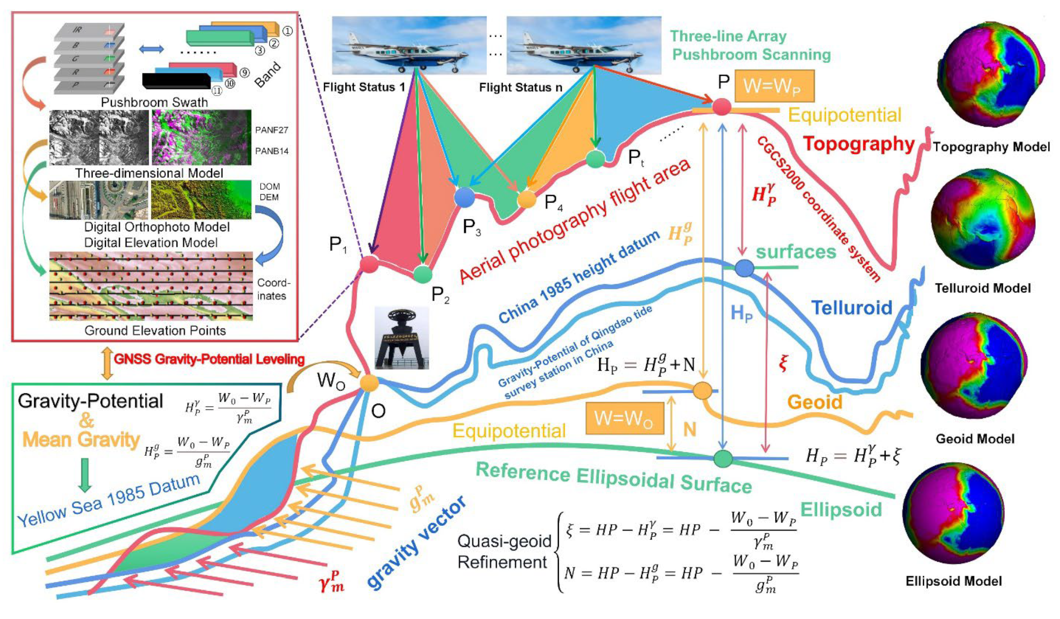
Figure 2.
Distribution of regional and multi-source remote sensing imagery. The red lines delineate the primary active faults in the region. Earthquakes are marked using different colors corresponding to their magnitudes: green for MW ≥ 7.0, blue for MW 6.0-7.0, yellow for MW 5.0-6.0, and red for MW ≤ 5.0, which occurred between 1902 and 2023 [23]. The coverage areas of Sentinel-1A, GF2, and GF7 satellite imagery are outlined by yellow and blue rectangles, respectively. The extent of the study area is indicated by a cyan-filled rectangle.
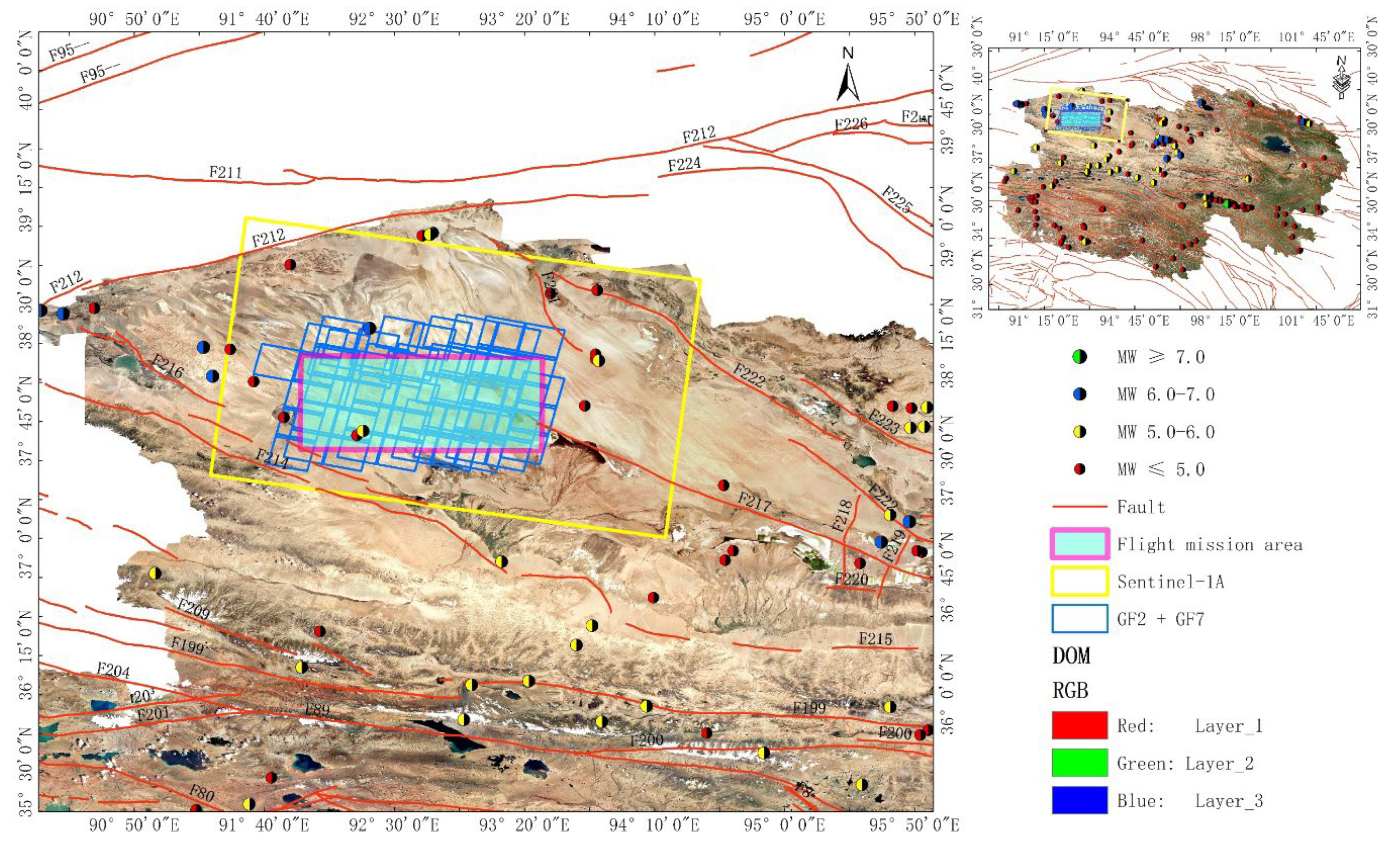
Figure 5.
Analysis of the precision in PPK data processing, (a) Observational status of the five satellite systems, including GPS, GLONASS, BeiDou, and Galileo, (b) DD_DOP values across all satellite observation periods. (c) Residuals for a subset of satellite observation fits. (d) Operational performance of the PAV80 tri-axial stabilization platform during the flight. (e) Breakdown of the aircraft’s velocity components during flight. (f) Stability of the aircraft’s flight altitude. (g) Precision of POS data obtained from the fusion of IMU (roll φ, pitch Ω, yaw κ) and GNSS (X, Y, Z) readings. (h) Adjustments to the Roll, Pitch, and Azimuth (Az) values. (i) Residuals following the transformation of the forward flight velocity components to the E, N, and U directions.
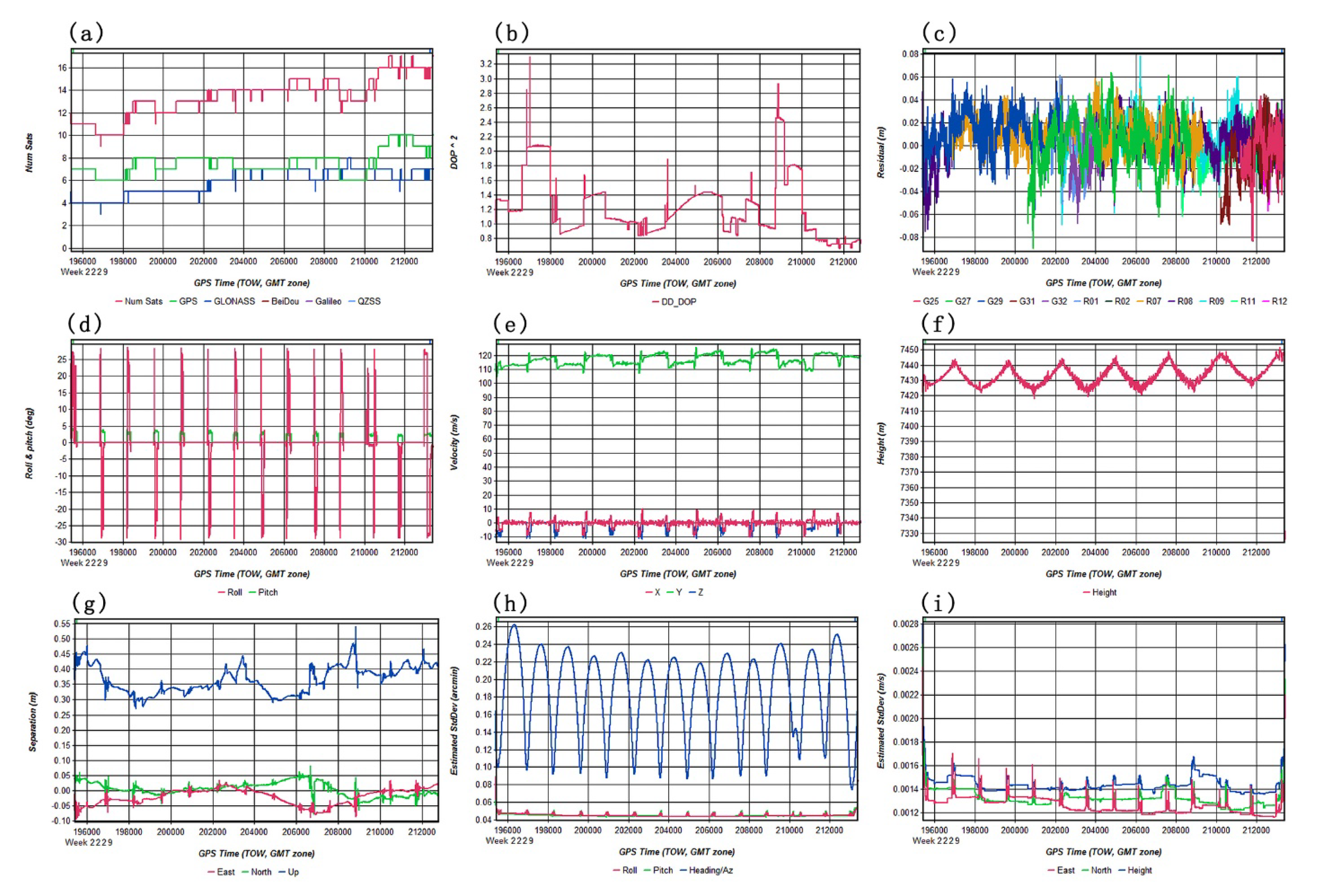
Figure 6.
Spatial distribution of GCPs and checkpoints for aerial triangulation. Illustrate the various GCP layout schemes, with red triangles representing the GCPs and green triangles denoting the checkpoints. Depict the deployment of GCPs in various environments within the study area.
Figure 6.
Spatial distribution of GCPs and checkpoints for aerial triangulation. Illustrate the various GCP layout schemes, with red triangles representing the GCPs and green triangles denoting the checkpoints. Depict the deployment of GCPs in various environments within the study area.
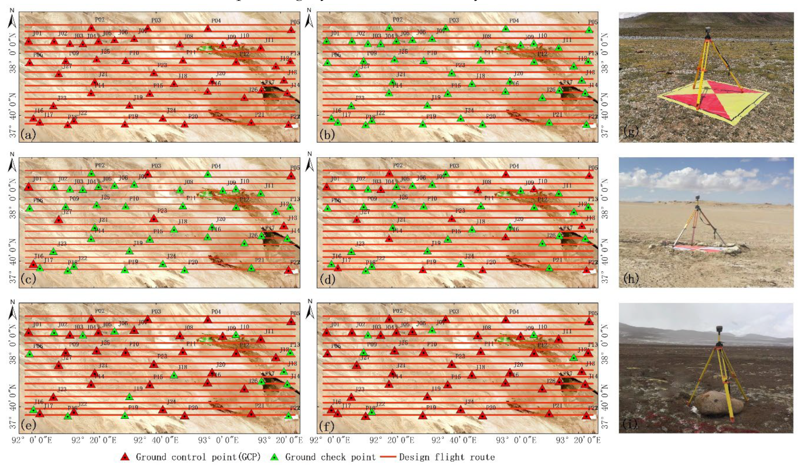
Figure 7.
Presents the Accuracy Analysis of Five Aerial Triangulation Densification Schemes. (a), (c), (e), (g), and (i) depict the horizontal MSE values for control and checkpoint distribution in Control Point Deployment Schemes I through V. Blue circles represent the MSE of control points, with the cyan line illustrating the fitted curve for the control points’ MSE. Red circles indicate the MSE of checkpoints, with the magenta line representing the fitted curve for the checkpoints’ MSE. Conversely, (b), (d), (f), (h), and (j) display the vertical MSE values for control and checkpoint distribution across the same deployment schemes. Here, magenta circles denote the control points’ MSE, accompanied by a cyan fitted curve, while green circles indicate the checkpoints’ MSE, with a magenta fitted curve for these errors as well.
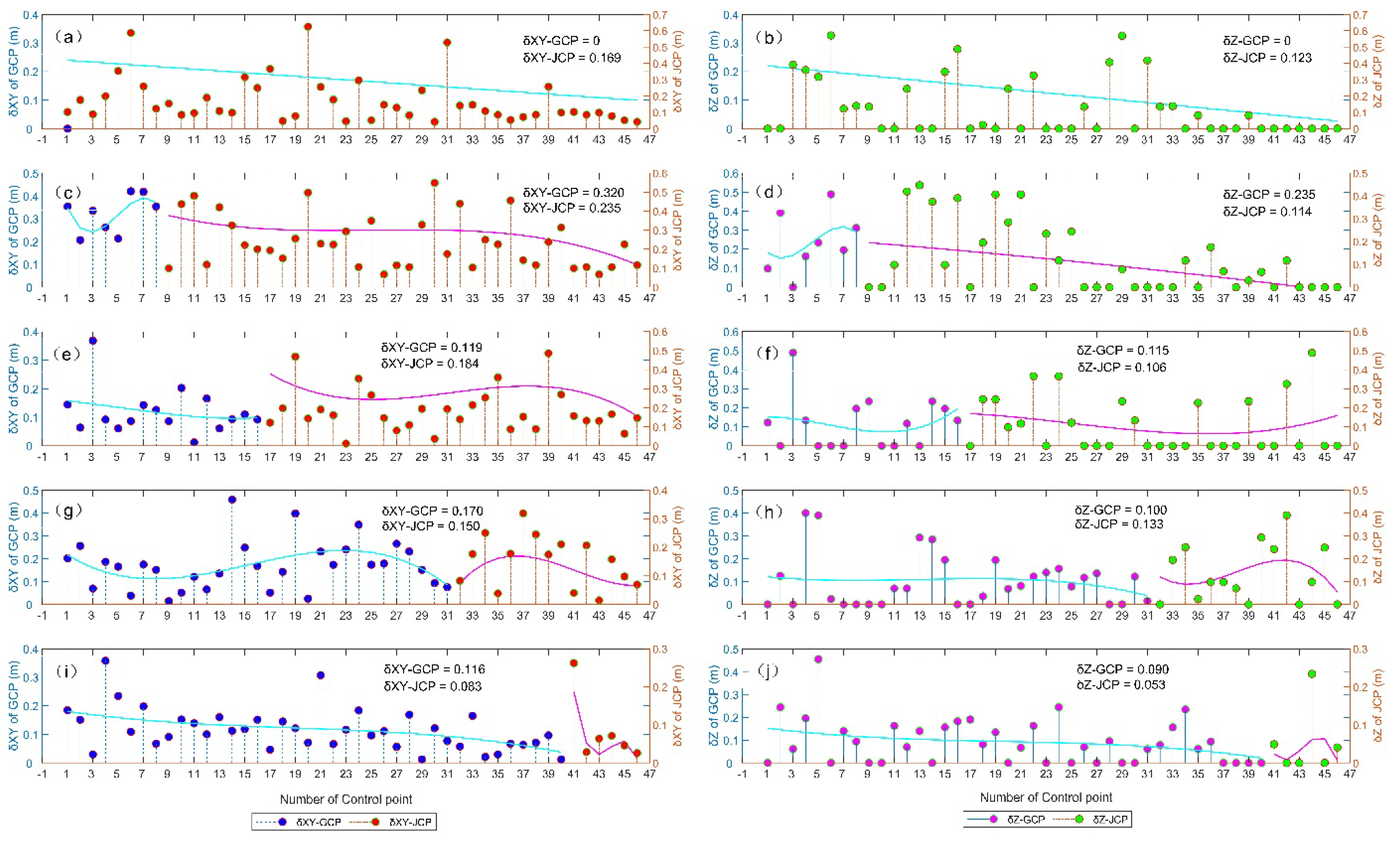
Figure 8.
Illustrates the retrieval of ground elevation points within a 3D stereoscopic environment and their spatial distribution across the surveyed region. Panel (a) delineates the three employed stereoscopic image display modalities: Pattern 1 corresponds to the Dual Stereoscopic Image Display Mode, Pattern 2 to the Anaglyphic Stereoscopic Image Display Mode, and Pattern 3 to the Polarized Light Stereoscopic Image Display Mode. Panel (b) features the key notations for interpreting the spatial data: red-black circles represent the Grid Points of the Foundation Quasi-geoid; yellow-black circles signify the Elevation Grid Points extracted within the 3D Stereoscopic Environment; and the black dots correspond to the actual POS points calculated post-flight.
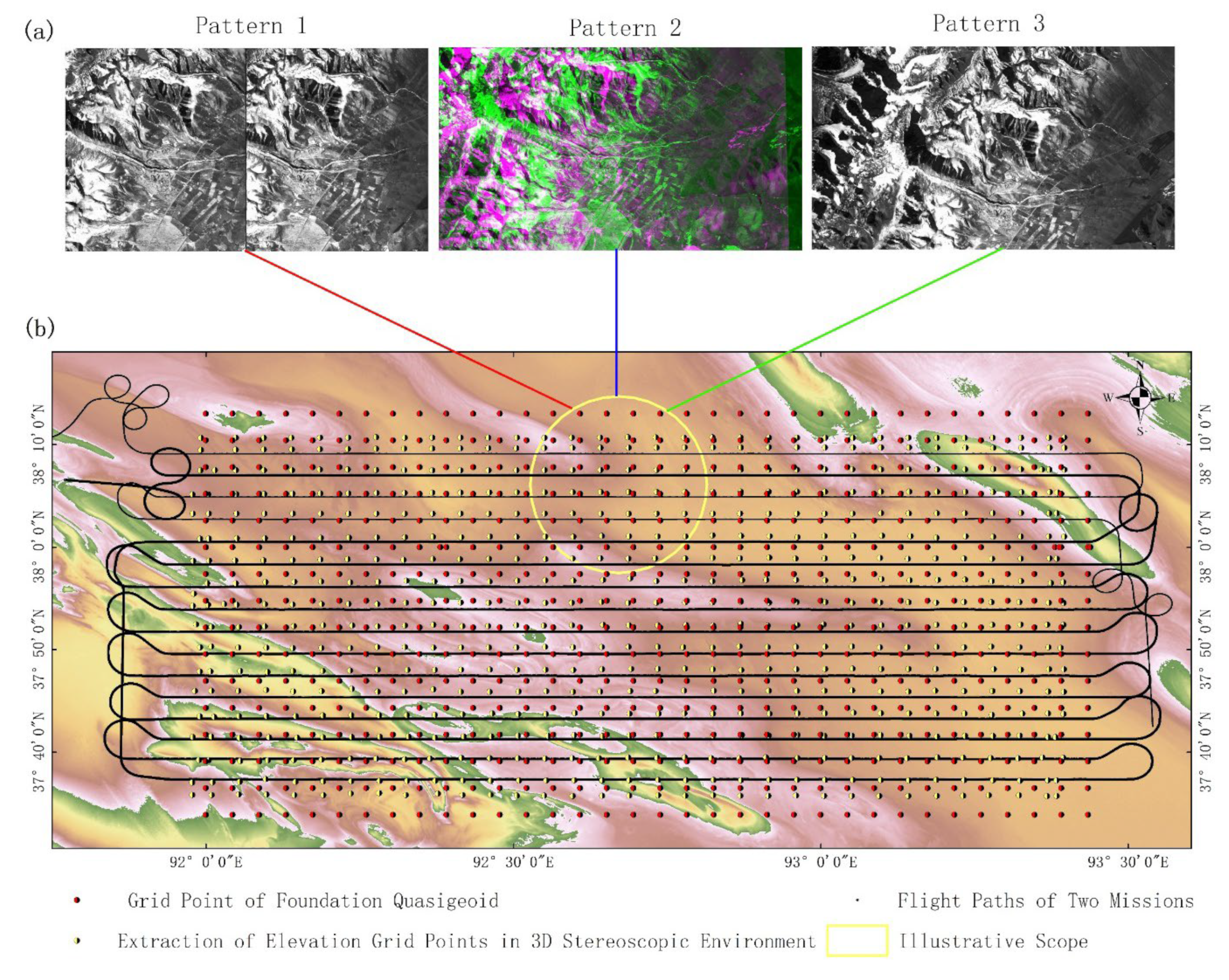
Figure 10.
Evaluation of the Accuracy of Different Gravity Potential Models. (a) Elevation residual values for GNSS points captured by all 3D solid models, calculated from 12 gravity potential models. (b)- (m) RMSE values of elevations for GNSS points captured by all 3D solid models, calculated from 12 gravity potential models.
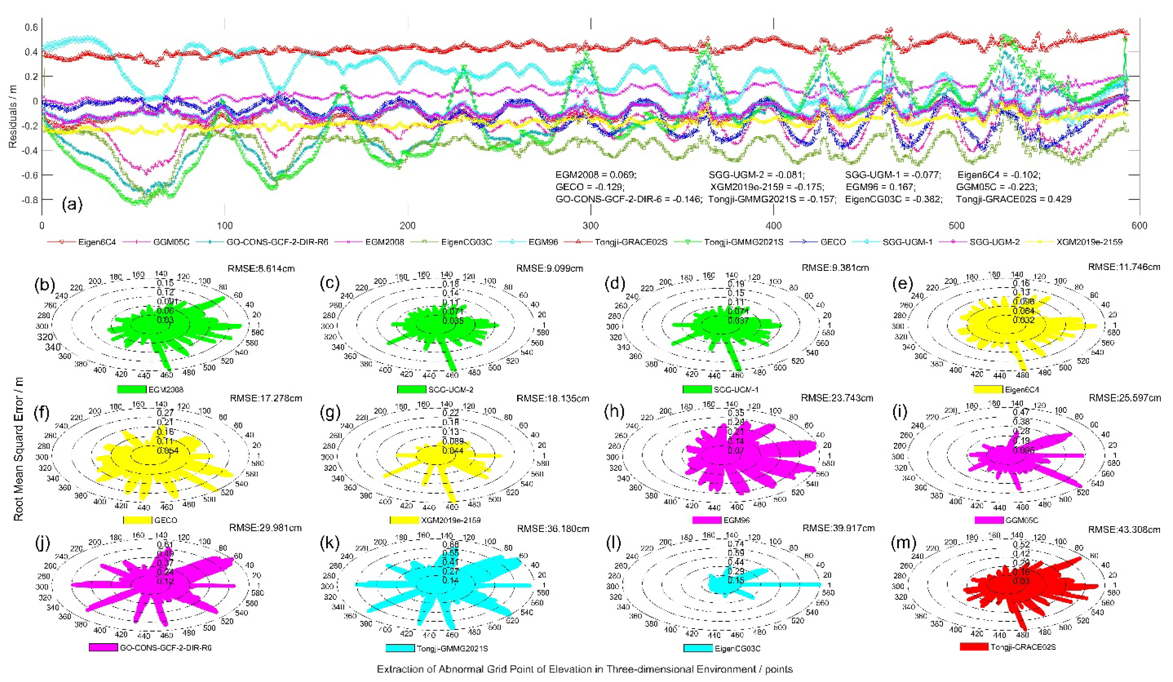
Figure 11.
Precision Analysis of Height Anomalies. (a) Estimation of the Quasi-Geoid Model in the Study Area Based on GNSS-Leveling Integration. Namely (a1)–(a12) The Quasi-Geoid Models for the Study Area Fitted with Height Anomalies Calculated from Twelve Gravitational Models. (b) RMSE Values for Height Anomalies Calculated Using the Twelve Gravitational Models.
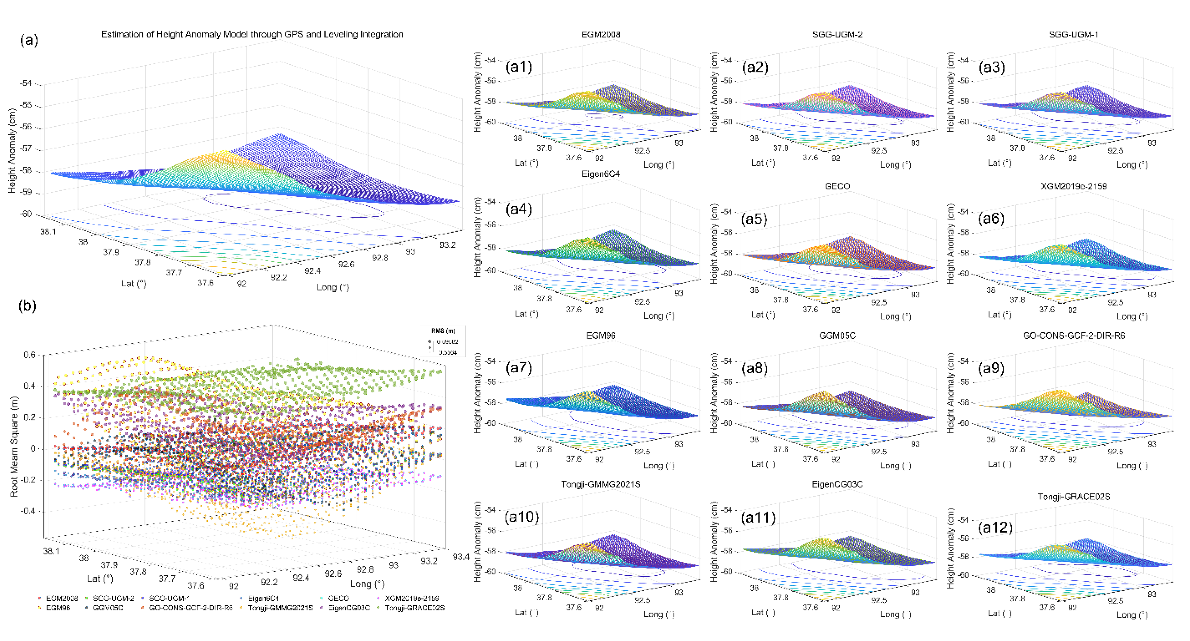
Figure 12.
RMSE Values for Height Anomalies Calculated Using the Twelve Gravitational Models.
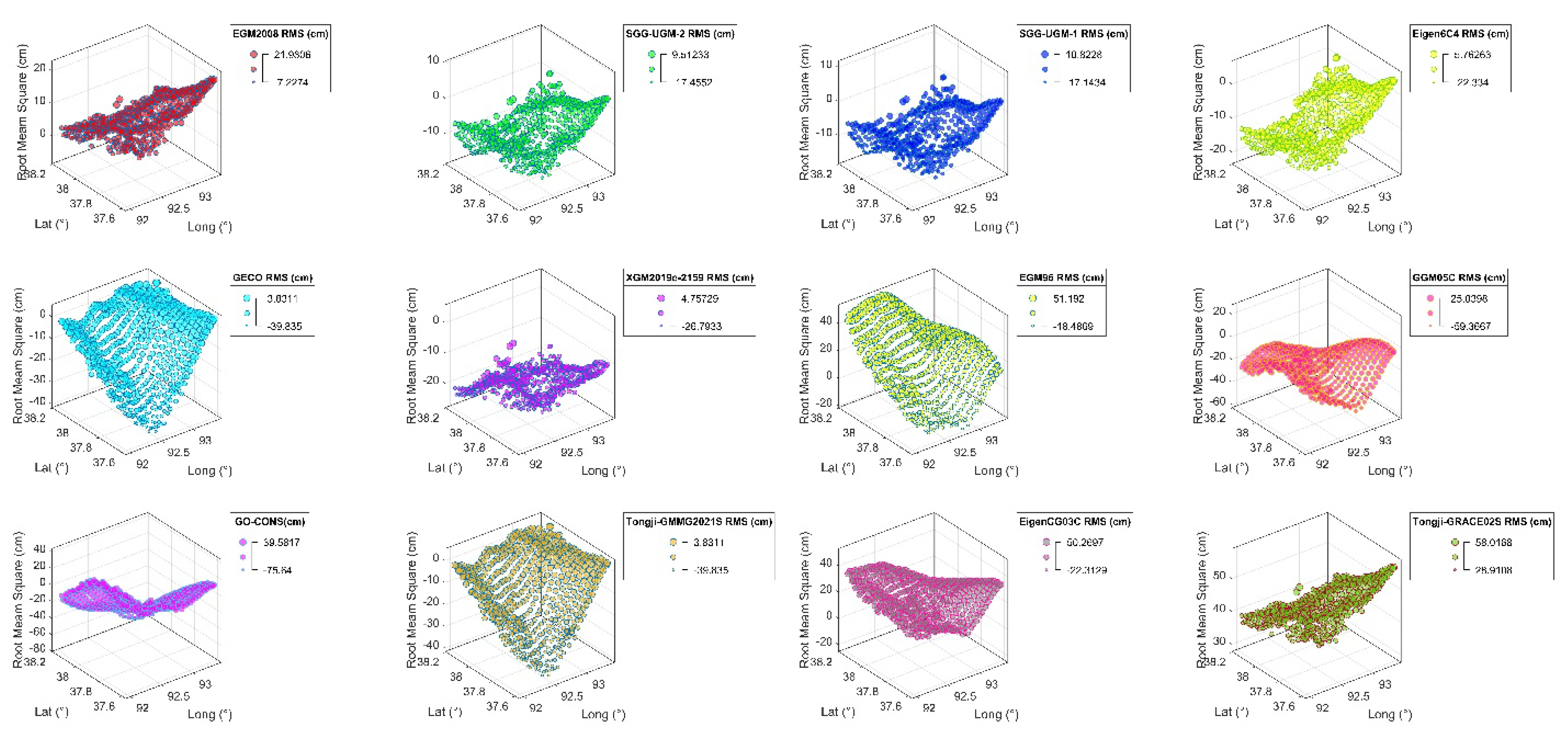
Disclaimer/Publisher’s Note: The statements, opinions and data contained in all publications are solely those of the individual author(s) and contributor(s) and not of MDPI and/or the editor(s). MDPI and/or the editor(s) disclaim responsibility for any injury to people or property resulting from any ideas, methods, instructions or products referred to in the content. |
© 2024 by the authors. Licensee MDPI, Basel, Switzerland. This article is an open access article distributed under the terms and conditions of the Creative Commons Attribution (CC BY) license (http://creativecommons.org/licenses/by/4.0/).
Copyright: This open access article is published under a Creative Commons CC BY 4.0 license, which permit the free download, distribution, and reuse, provided that the author and preprint are cited in any reuse.


