Submitted:
27 June 2024
Posted:
27 June 2024
You are already at the latest version
Abstract
Compared to traditional multi-robot path planning problems, multi-chain robot path planning (MCRPP) is more challenging because it must account for collisions between robot units and between the bodies of a chain and the leading unit during towing. To address MCRPP more efficiently, we propose a novel algorithm called Multi-Train Safe Interval Path Planning (MT-SIPP). Based on safe interval path planning principles, we categorize conflicts in the multi-train planning process into three types: travel conflicts, waiting conflicts, and station conflicts. To handle travel conflicts, we use an improved k-robust method to ensure trains avoid collisions with other trains during movement. To resolve waiting conflicts, we apply a time correction method to ensure the safety of positions occupied by trains during waiting periods. To address station conflicts, we introduce node constraints to prevent other trains from occupying the station positions of trains that have reached their target stations and are stopped. Experimental results on three benchmark maps show that the MT-SIPP algorithm achieves about a 30% improvement in solution success rate and nearly a 50% increase in the maximum number of solvable instances compared to existing methods. These results confirm the effectiveness of MT-SIPP in addressing the challenges of MCRPP.
Keywords:
Multi-chain robot
; path planning
; travelling conflicts
; waiting conflicts
; station conflicts
1. Introduction
Intelligent robots are increasingly applied in smart environments, capable of autonomously or semi-autonomously performing diverse tasks through instruction reception and execution. Particularly in scenarios necessitating multiple robots to cooperatively reach different target locations for task execution, such as in logistics [1,2], agriculture [3], and factory handling [4,5], the technology of Multi-Agent Path Finding (MAPF) [6] becomes pivotal. This technology aims to devise optimal and collision-free paths from starting points to target points for each robot, while ensuring safety during the movement process.
In pursuit of this objective, researchers have extensively explored the field of MAPF [7,8,9], introducing a variety of planning algorithms [10,11,12] tailored to diverse path planning needs. Among these, Sharon et al. [13] proposed the Conflict-Based Search (CBS) algorithm, which has made significant strides in achieving optimal and comprehensive solutions for MAPF. CBS utilizes a conflict constraint tree to expand nodes, detecting conflicts and imposing constraints based on optimal single-agent path planning. It subsequently replans conflicting robots within existing constraints until conflict-free paths are established. In order to further enhance the efficiency of the CBS algorithm, Boyarski et al [14] improved strategies for conflict priority and meta-agents, which effectively reduced the number of conflicting nodes. Additionally, Ariel et al. [15] optimized the node expansion process within the CBS algorithm by introducing the Add Heuristics to Conflict-Based Search (CBSH) algorithm. By integrating heuristics as reference metrics for node selection during high-level node expansions, CBSH effectively reduces the number of expanded nodes, thereby accelerating the solving process. Building on the CBSH algorithm, Li et al. [16] addressed the issue of long processing times for handling rectangle conflicts. By introducing different methods to infer and add rectangle conflict constraints, Li effectively reduced invalid or redundant node expansions, thereby further improving the solving efficiency of the CBSH algorithm.
Taking into account potential delays encountered by robots during actual movement, Dor et al. [17] introduced the k-Robust Conflict-Based Search (kR-CBS) algorithm. This algorithm allocates a safety margin of time steps for each path node during planning, ensuring robots can safely execute tasks even when delays of up to time steps occur. This proactive approach effectively mitigates potential collision risks. To tackle the challenge of exploring large path node spaces in coupled algorithms for multi-agent planning, Phillips et al. [18] introduced the Safe Interval Path Planning (SIPP) algorithm. This method prioritizes sequential planning of multiple robots based on their respective priorities. As robots complete their planning, they dynamically update safe intervals on the map grid, guiding subsequent robots in selecting path nodes. This decoupled and priority-driven approach ensures conflict-free paths once all robots have finalized their plans, significantly enhancing overall solving efficiency. However, Yakovlev et al. [19] identified a limitation in the SIPP algorithm during node expansion, where each grid node permits passage for only one robot at a time, potentially resulting in scenarios where solutions are not achievable. Therefore, he introduced a Weighted Safe Interval Path Planning algorithm that maintains optimal and suboptimal nodes during path node expansion. If the optimal node path cannot be expanded further, the algorithm leverages suboptimal nodes to improve solution success rate and adaptability.
The mentioned MAPF algorithms exhibit adaptability for robots occupying single grid nodes. For chain robots like trains and serpentine robots [20], which occupy multiple grid nodes [21,22], Dor et al. [23] defined the Multi-Train Path Finding (MTPF) problem and introduced the Multi-Train CBS (MT-CBS) algorithm. Chen et al. [24], building upon MT-CBS, further developed MT-CBS, MT-ICBS, MT-CBSH, and MT-CBSH-RM to offer a more comprehensive solution for chain robot path planning. However, CBS-type algorithms primarily rely on node search and splitting mechanisms, limiting their scalability for large-scale MTPF problems. In contrast, the SIPP algorithm uses safe intervals as its planning foundation, enabling simultaneous detection and setting across multiple consecutive time steps, thus ensuring higher search efficiency. Despite the existence of the MT-CBS algorithm [23] for addressing MTPF problems, research leveraging SIPP algorithm principles for MTPF remains relatively scarce.
Our work aims to fill this gap and substantially reduce the computational complexity of pathfinding for chain robots, thereby improving the success rate in solving large-scale MTPF problems. Building upon the principles of the Safe Interval Search Algorithm, we have devised a novel planning strategy termed the Multi-Train Safe Interval Path Planning (MT-SIPP) algorithm. Our MT-SIPP incorporates robust techniques [17] to address conflicts during locomotion, adjusting vehicle occupancy time steps in grid during wait conflicts, and employing checks on train stop grids and the addition of node constraints to manage stopping conflicts. MT-SIPP guarantees swift generation of effective paths for multiple trains within defined time constraints.
2. Problem Description
2.1. Multi-Agent Path Finding
Multi-agent path finding [6] is a technique for planning paths for multiple robots in an undirected graph , aiming to find a path from the start point to the end point for each robot within the obstacle-free region R. Here, represents the grid node, and represents the edges connecting the grid. During the planning process, the robot typically occupies only one grid at time step , and the complete path is defined as , where denotes the grid position of robot at , and represents the total time cost required for robot to reach the destination. To ensure the effectiveness of planned paths, the returned path nodes must adhere to the following constraints:
Where, Equation (1) guarantees that all robot movements are strictly constrained within the non-obstacle region, ensuring the selected path nodes' navigability and safety. Equation (2) effectively prohibits two robots from occupying the same grid node simultaneously, thereby preventing potential vertex conflicts. Equation (3) avoids situations where two robots traverse the same edge of a grid node simultaneously at the same time step, thus eliminating the possibility of edge conflicts. Furthermore, based on potential conflict scenarios among multiple robots, these can be categorized into vertex conflicts and edge conflicts. Vertex conflicts occur when two robots occupy the same grid node simultaneously, as depicted in Figure 1(a). On the other hand, edge conflicts arise when two robots attempt to traverse the same edge of a grid node simultaneously, as shown in Figure 1(b).
2.2. Multi-Train Path Finding
Multi-train path finding differs significantly from MAPF in its approach to handling chain-like robots. For robots with a body length of , as they depart from the starting point, the number of grid they occupy gradually expands from 1 to . Specifically, if a robot's head occupies grid at time step , its body also occupies nodes such as where are the grid previously traversed by the robot's head, and these nodes constitute the "car_body". The path of the multi-train robot i is represented as . The core objective of MTPF algorithms is to identify a set of path sets, ensuring all robot paths are collision-free, and minimizing the total cost sum of all paths. This necessitates the algorithm to consider not only the optimal path for each individual robot during planning but also to coordinate path selections among multiple robots to achieve global optimality.
MTPF Objectives:
MTPF Constraints:
Where, denotes the number of chain robots, and SOC refers to the aggregate cost in time for all chain robots to reach their target points individually. Equation (5) ensures unrestricted movement of all chain robots within non-obstacle regions. Equation (6) specifically addresses the characteristics of chain robots, whose bodies (comprising multiple grid of their head and body) must not occupy the same grid simultaneously as any part of another chain robot during movement, thereby preventing point conflicts.
Notably, since chain robots occupy multiple contiguous grid during movement, the MTPF problem avoids edge conflict scenarios that could arise in MAPF, such as when two chain robots might swap positions, as depicted in Figure 2.
3. SIPP Algorithm
The Safe Interval Path Planning (SIPP) algorithm innovatively extends the classical A* algorithm [25] by incorporating the concept of safe intervals. In this algorithm, each grid cell is pre-defined with a global safe interval list. For example, obstacle grid cells have an empty safe interval list, while unvisited grid cells initially possess an initial safe interval list , indicating safe accessibility at any time. During MAPF, each robot evaluates whether to add expanded grid cells to the OPEN list based on their respective safe interval lists. This mechanism enables precise node selection, significantly reducing unnecessary node expansions. After successful path planning for multiple robots, they backtrack from their respective target nodes to generate individual paths. Subsequently, the SIPP algorithm updates the global safe interval lists of involved grid cells in these paths to ensure subsequent planning robots can avoid conflicts and select nodes based on updated safe interval information.
Consider one non-obstacle grid with a safe interval list in Figure 3 as an example. Following the completion of multi-robot planning, assuming Robot 1 passes through grid cell A at time step 3, and Robot 2 passes through the same grid cell at time step 5. Based on this information, the safe interval list for this grid cell will be updated to , effectively representing its availability across different time periods. This mechanism illustrates how the SIPP algorithm offers a clear and efficient conflict avoidance strategy for subsequent robot planning.
4. K-. Robust Planning Methods
As referenced in [17], to mitigate potential delays encountered by robots during path execution, an effective strategy involves preemptively accounting for delay factors during the planning stage and assigning suitable safety buffers for each robot. This measure significantly enhances the robustness of multi-robot path planning, enabling it to withstand delays to a certain extent. In practical implementation, since most multi-robot path planning algorithms expand nodes based on integer time steps, K-robust planning algorithms typically simplify computations by setting as an integer value. For instance, in Figure 4, if Robot 1 is allocated a safety buffer of 1 time step during the planning phase (i.e., )), and Robot 1 passes through grid at time step 3 while Robot 2 passes through the same grid at time step 5, the safe interval for grid A would accordingly update to . This updating strategy ensures that robots can traverse grids safely and sequentially according to their planned paths, even in the presence of potential delays.
Upon comparing Figure 3 and Figure 4, we can clearly discern the practical application effects of the -robust planning algorithm. This algorithm effectively extends the time duration that a robot occupies a grid from a single time step to + 1 time steps. Therefore, if Robot 1 or Robot 2 encounters a delay of up to time steps upon leaving grid A, they may potentially remain on grid A during these time steps. To mitigate this scenario, the -robust planning algorithm assigns a safety buffer of time steps for these robots. This approach treats the subsequent time steps as collision intervals during planning, effectively preventing other robots from passing through grid A within time steps. Such a strategy ensures that Robot 1 and Robot 2 can safely execute their path planning even in the presence of delays, thus minimizing potential collisions and conflicts.
5. MT-SIPP Algorithm
Based on the SIPP algorithm [18], this paper extends its application to multi-train path planning. The MT-SIPP algorithm categorizes potential conflicts into three types when planning paths for multiple trains: train movement conflicts, waiting conflicts, and station stopping conflicts. To effectively address these conflicts, the algorithm employs the following strategies:
(1) For movement conflicts, the MT-SIPP algorithm employs an improved K-robust method. This approach ensures that trains maintain sufficient safety distances during their movement, effectively preventing collisions with other trains.
(2) When facing waiting conflicts, the algorithm utilizes time adjustment techniques. By appropriately adjusting the waiting times of trains, this method ensures that the track positions occupied by waiting trains remain unobstructed by others, thereby ensuring the safety of waiting trains.
(3) Addressing station stopping conflicts, the MT-SIPP algorithm implements strategies such as adding node constraints. These strategies ensure that when a train reaches and stops at its destination station, other trains do not occupy or block its stopping position, thereby mitigating station stopping conflicts.
5.1. Train Movement Conflicts and Resolution Methods
5.1.1. Definition of Conflict
Train movement conflicts refer to collisions or overlaps between the bodies of two trains during their traction and movement. This occurs when parts of two or more trains occupy the same grid simultaneously, denoted as . In train path planning, the process typically revolves around planning based on the train head and indirectly inferring the body's movement path through the head's trajectory. However, this simplified approach may lead to potential conflicts. To completely avoid such conflicts, it is essential to consider the paths of entire trains, especially when updating safety intervals.
Figure 5.
Schematic diagram of train collision. (a) Status 1; (b) Status 2.
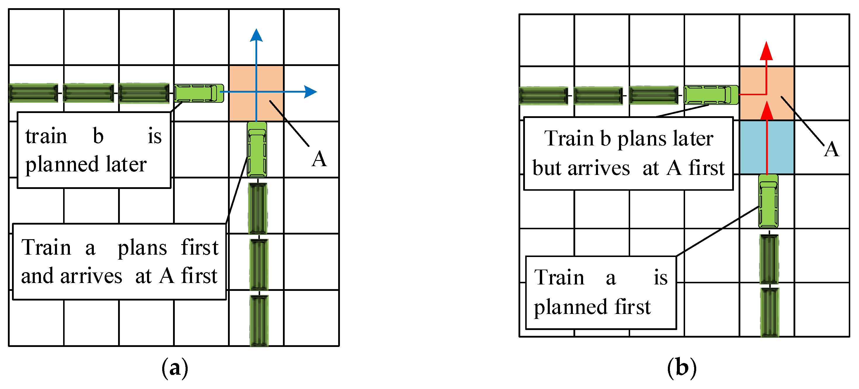
As depicted in Figure 5(a), if no additional time step constraints are imposed on the orange grid traversed by train a during its head path planning, there is a risk that train b could enter the same grid immediately after train a's head has departed. This scenario may lead to a collision between train a's body and train b. Similarly, in Figure 5(b), without additional time step constraints on the orange grid along train a's head path, when train a's head reaches the blue grid, train b's head might occupy the orange grid. Even if train b's head has already vacated the orange grid before train a arrives, the presence of train b's body in the area could still result in a collision between the two trains. Therefore, to prevent train movement conflicts, it is essential to comprehensively consider the paths of entire trains during the planning process and apply appropriate time step constraints to grids where conflicts may occur.
5.1.2. Conflict-Free Strategy
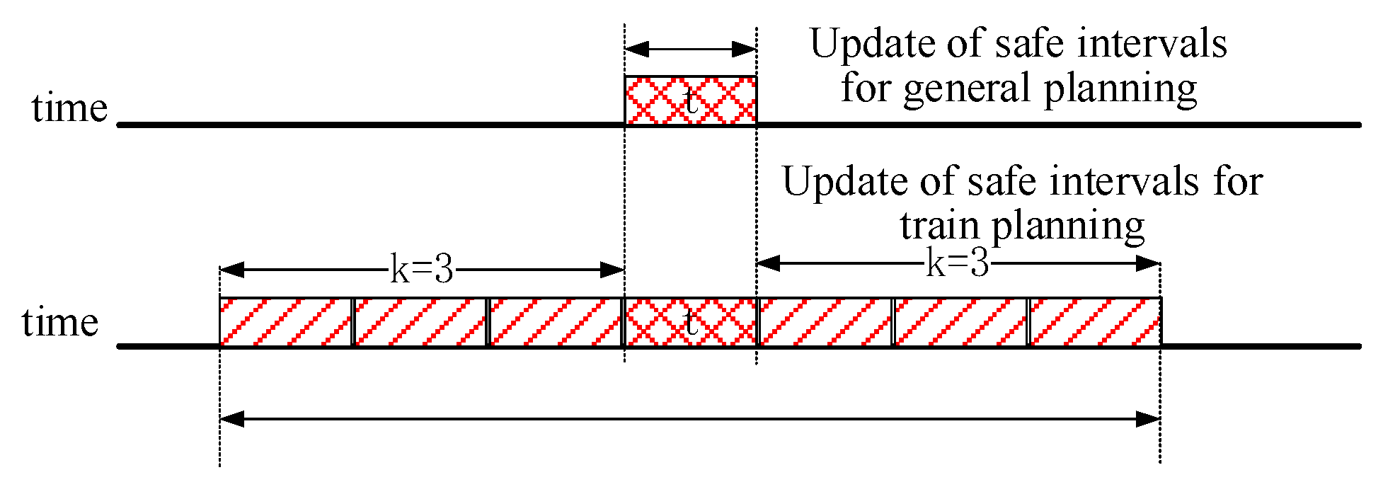
In addressing the train movement conflicts outlined in Section 5.1.1, this paper proposes the adoption of an enhanced K-robust method [17] to effectively mitigate these conflicts. As depicted in Figure 6, during the progression of a train, once its head traverses a grid (designated as grid x), the system automatically designates all time steps from to (specifically, ) as collision intervals for that grid. This precaution prohibits other trains from passing through the grid during this defined time window, thereby ensuring robust prevention of train movement conflicts.
This strategy ensures that during the movement of the current train, its body will be completely cleared from the current occupied grid after time steps. Alternatively, if another train has passed through and vacated the grid before k time steps, the current train's body can also be fully cleared from the grid occupied by its head within time steps. This approach effectively prevents collisions between two trains during their movement.
By setting collision interval constraints for grids traversed by the current planned train, we ensure that after completing the current train's planning phase, no other train passes through within grids behind or ahead of it. This measure effectively mitigates the risk of the train's body colliding with other trains or being collided with during its movement.
Figure 6.
Schematic diagram of the improved robust method for resolving train travel conflicts.
The following is a segment of pseudocode for identifying successor nodes at time step that satisfy the robust safety criteria for trains within time steps:
| Function1: get_k_robust_successors() |
| 1:=get_neighbors() |
| 2:for in do |
| 3: for in do |
| 4: if && then |
| 5: ), append |
| 5: end if |
| 6: end for |
| 7:end for |
| 7:return |
Obtaining nodes that satisfy the robust conditions is essential, yet insufficient to ensure absolute conflict-free operation between trains. To safeguard system integrity, it is imperative to methodically update the safety intervals of grid encompassed by planned paths following successful planning completion. This practice prevents inadvertent occupation of already allocated safety intervals during node expansion in subsequent planning phases, thus effectively preempting potential conflicts.
5.2. Train Waiting Conflicts and Resolution Methods
5.2.1. Definition of Conflict
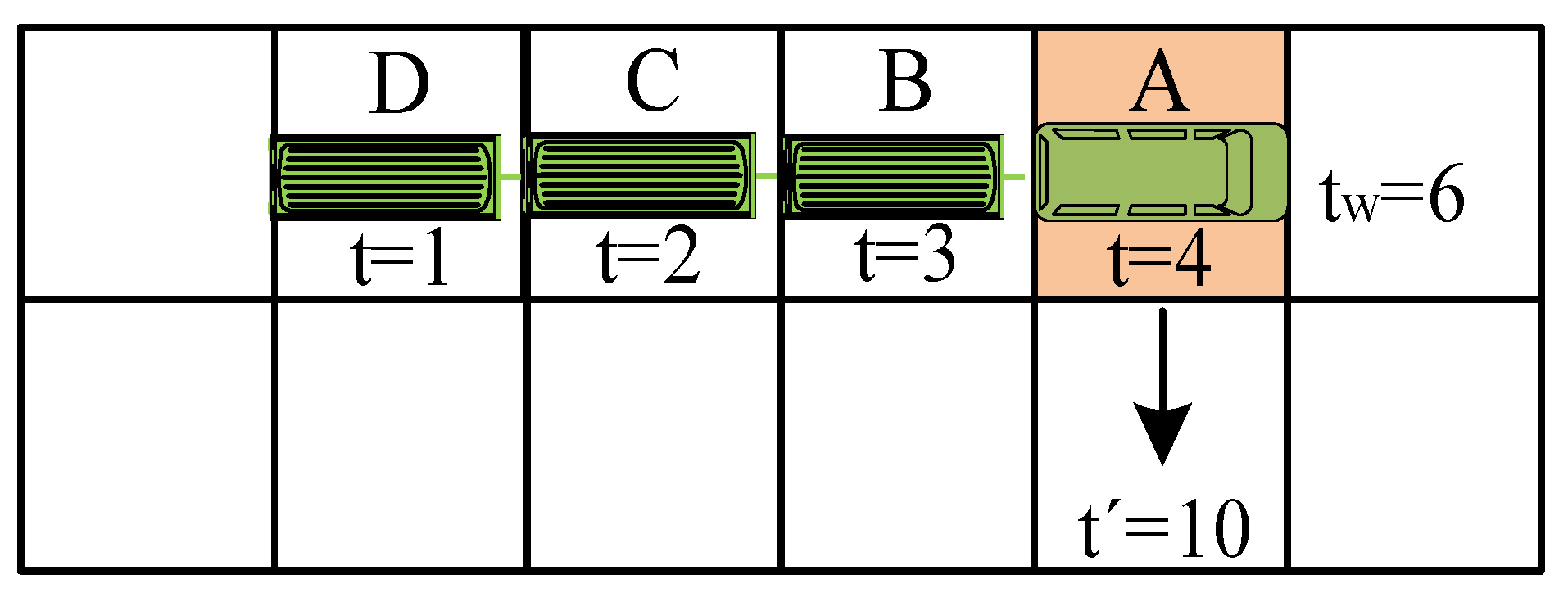
Train waiting conflicts occur when a train, during its journey, is forced to halt and wait due to obstruction by another train. Improper handling of such situations can lead to a phenomenon where multiple cars of the halted train occupy the same grid simultaneously. As depicted in Figure 7, when applying an improved k-robust method to update safety intervals (with ), the train's locomotive occupies grids D, C, B, A at consecutive time steps respectively. Under normal conditions, at time step , while the locomotive occupies grid A, the train's three cars are positioned on grids B, C, D. According to the k-robust method, to prevent conflicts, the system restricts other trains from passing through grids D, C, B, A during time steps 1 to 4, 1 to 5, 1 to 6, and 1 to 7, respectively. However, complications arise when a train waits at grid A for 6 time steps (until ) before resuming its journey. Despite the enhanced k-robust method prohibiting other trains from passing through grids D, C, B, A during time steps 1 to 4, 1 to 5, 1 to 6, and 1 to 13, in such cases, the train's cars remain stationary on their original grids from time steps 7 to 9, leading to a lapse in collision avoidance intervals. This indicates that if another train attempts to pass through grids D, C, B during time steps 5 to 10, 6 to 11, 7 to 12, collisions may potentially occur.
Hence, to prevent such waiting conflicts, it is imperative to incorporate additional temporal constraints into the train waiting process. This measure ensures that, even during train halts, other trains are prevented from accessing grids where collisions could occur, thereby comprehensively enhancing system safety.
Figure 7.
Schematic diagram of train waiting.
5.2.2. Conflict-Free Strategy
To address train waiting conflicts, this paper proposes a time-step adjustment method designed to effectively prevent collisions between trains during waiting periods. Upon completion of route planning and safety interval updates at the train head, we analyze the positional relationship of adjacent path nodes to identify instances where the train is waiting at specific locations. We calculate the waiting duration () based on the cost differential between these adjacent nodes.
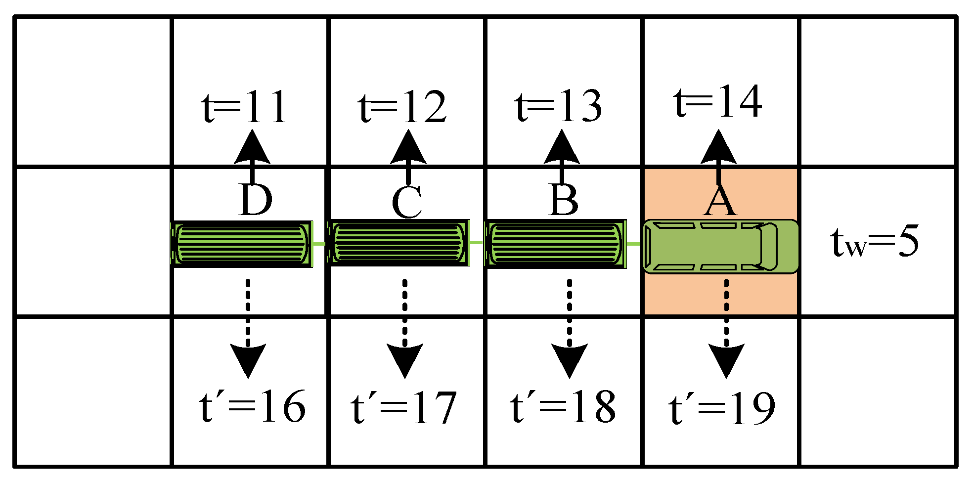
Specifically, if nodes node_a and node_b are consecutive path nodes where node_a_position equals node_b_position, this indicates that the train is waiting at node_b's position. The waiting time can be determined by calculating the difference between node_b_g (the cost of node_b) and node_a_g (the cost of node_a). When updating the safety interval of the train head, if the head waits for time steps at a certain time step, the corresponding time that the train body occupies adjacent grids will also extend by time steps. Since the grids occupied by the train body are those the train head has already passed through, adjusting the time the train body occupies these grids essentially adjusts the time the train head passed through them. To determine the grids occupied by the train body during waiting, we trace back from the current position of the train head while excluding the waiting path nodes. Ultimately, the time steps at which the train head passes through the grids occupied by the car will be adjusted from the original to . As illustrated in Figure 8, suppose a train of length (where ) passes through grids D, C, B, A at time steps 11, 12, 13, 14 respectively, and waits at grid A for 5 time steps until time step 19, still occupying grid A. To prevent conflicts, the time steps during which the train head passes through grids D, C, B need adjustment to 11 to 16, 12 to 17, 13 to 18. Consequently, other trains will be prohibited from passing through the corresponding grids during time steps , , .
Through this approach, we can introduce supplementary temporal constraints on the grids occupied by the train body during its waiting periods. This effectively prevents other trains from traversing these grids while the train is in a state of wait, thereby preempting potential collisions.
Figure 8.
Time step adjustment of the car body occupying the grid when the train front is waiting.
Before updating the safety interval list following successful single-machine planning, the pseudocode for identifying waiting nodes in the path and implementing time-step adjustment to prevent waiting conflicts is outlined as follows:
| Function2: detection_and_correction_of_waiting_nodes() |
| 1:=make_path() |
| 2:for in do |
| 3: update_safe_interval() |
| 4: if = then |
| 5: =- |
| 6: =get_car_body() |
| 7: for in do |
| 8: for in (,+) do |
| 9: =(,) |
| 10: update_safe_interval() |
| 11: end for |
| 12: end for |
| 13: end if |
| 14:end for |
To effectively prevent waiting conflicts after successful single-machine planning, we identify waiting nodes in the path before updating the safety interval list and implement time-step adjustments. This method is selected for two primary reasons: first, to avoid unnecessary checks for waiting conflicts and unnecessary time-step adjustments for every expanded node during the planning process, thereby reducing computational complexity and improving solution efficiency; second, because in single-machine planning, although many nodes are expanded, not all nodes ultimately contribute to the final path. Only those nodes selected to form the final path are considered genuinely significant.
5.3. Train Station Stop Conflicts and Resolution Methods
5.3.1. Definition of Conflict
Train station stop conflicts refer to situations during train operations where, for various reasons, one train attempts to stop at a station but encounters positional conflicts with another train. These conflicts primarily encompass three scenarios: firstly, the train's body occupies the destination point intended for another train after it has stopped (i.e., and ); secondly, the planned stopping position of the train is already occupied by another train; thirdly, after stopping, the train's body completely obstructs another train's path to its destination point.
During train head path planning, failure to adequately consider the actual grid occupation by the train body can lead to station stop conflicts, even when the target points of two trains differ. Figure 9(a) illustrates the first conflict scenario where the body of train 1 occupies the target point of another train after stopping, directly preventing the other train from stopping as planned and causing planning failure. Figure 9(b) shows the second conflict scenario where the planned stopping position of train 2 is already occupied by another train, similarly leading to planning failure for train 2. Figure 9(c) depicts the third conflict scenario where, in narrow settings, one train completely obstructs another train's path to its target point after stopping, resulting in planning failure for the obstructed train. To mitigate these station stop conflicts, it is essential to fully consider the actual grid occupation by the train body during the path planning phase. This consideration should also encompass the relative positions and operational timings with respect to other trains, ensuring safe and efficient station stops and operations.
5.3.2. Conflict-Free Strategy for Status 1 and Status 2
To effectively mitigate station stop conflicts described in scenarios 1 and 2, this study employs a strategy that combines grid position checks for parking and the addition of node constraints. When planning the path for each train to reach its destination point, the system traces back several preceding path nodes before the target point to determine the specific grid range occupied by the train body upon arrival (referred to as car_position). Subsequently, the system checks whether car_position intersects with the destination points of other trains (stored in the GOALS list) or grids occupied by already stopped trains (stored in the CARS list). If or , it signifies that stopping at the current extended path node would lead to conflicts with other trains. In such cases, the algorithm discards the current node and continues exploring other potential path nodes until finding a car_position that neither overlaps with any destination points in the GOALS list nor with grids occupied by stopped trains in the CARS list (i.e., and ). This ensures that the current train can safely stop at that node. The algorithm retains this path node for subsequent backtracking and generation of a comprehensive conflict-free path.
It is noteworthy that nodes in the GOALS list are extracted during the algorithm initialization phase by reading map task information. In contrast, the CARS list requires dynamic updating after completion of each train's path planning phase. This involves backtracking from the target points to capture the grid positions occupied by the train body upon final station stop, ensuring real-time reflection of track occupancy.
The pseudocode for this process is as follows:
| Function3: resolve_station_stopping_conflict-1() |
| 1:if = do |
| 2: =get_car_position() |
| 3: if n ∩ { ∪ CARS}≠∅ then |
| 4: =get_best_node() |
| 5: = |
| 6: else |
| 8: = |
| 9: end if |
| 10:end if |
5.3.3. Conflict-Free Strategy for Status 3
To address the third type of station stop conflict as depicted in Figure 9, which cannot be preemptively detected during the initial train planning phase, we adopt a post-processing strategy. In cases where train 2 encounters a scenario where its path to the destination is entirely blocked by other trains during planning, we prioritize the planning of train 2. This prioritization ensures that train 2 is planned first, allowing train 1, which is planned subsequently, to make decisions based on train 2's path, either waiting for train 2 to reach its destination point before occupying its own destination point, or opting for an alternative path to avoid obstructing train 1's arrival.
To achieve this objective, this study employs a method for continuous multi-node endpoint conflict detection. In a priority-based multi-train path planning algorithm, whenever a train's leading node extends to reach a target point, we examine the value of the current extension node (which represents the time cost for the train to reach its target point) and assess whether other trains are scheduled to pass through the same target point subsequently. If the g-value of another train passing through the current train's target point (denoted as ) is less than or equal to the current train's value (i.e., ), it indicates a conflict. In such cases, we discard that node and continue expanding until we find a node with a value less than , indicating that no further trains are scheduled to pass through the current train's target point, thereby achieving successful planning.
In multi-train path planning, in addition to single-node conflict detection for each train's head, it is crucial to perform endpoint conflict detection for grids occupied by the connected train bodies along adjacent connections. This ensures that the current planned train can stop safely without obstructing previously planned trains that have already passed through its station grids, thus preventing potential collisions. However, in specific scenarios where prioritizing the planning of one train, such as train 2, inadvertently blocks another train, like train 1, from reaching its destination, it indicates a mutual constraint between the trains. To resolve this issue, when replanning train 1, we proactively add the stop position of train 2 from the previous planning round (referred to as car_position_2) to the constraint list. This ensures that when prioritizing the planning of train 1, the algorithm selects a stopping location that avoids occupying grids in car_position_2, thereby enabling train 2 to reach its destination unimpeded. Nevertheless, it is important to note that in highly congested and narrow scenarios where each train has only one viable path to its destination, mutual constraints between trains may render the algorithm unable to find a solution. In such cases, additional strategies or measures may be required to resolve these path conflicts effectively.
The pseudocode for this section is as follows:
| Function4: resolve_station_stopping_conflict-2() |
| 1:if = do |
| 2: =get_car_position() |
| 3: ←conflict detection(n) |
| 4: if = then |
| 5: ←get_best_node(OPEN) |
| 6: = |
| 7: else |
| 8: = |
| 9: end if |
| 10: if n ∩ ≠∅ do |
| 11: ←get best node(OPEN) |
| 12: = |
| 13: else |
| 14: = |
| 15: end if |
| 16:end if |
Finally, as depicted in Figure 10, following the completion of train planning, the system ensures operational safety and prevents future conflicts by excluding grids occupied by the train body after it reaches its final destination and extends its safety interval. This measure effectively prohibits other trains from passing through grids where a train has already halted, thereby maintaining safety intervals between trains and substantially mitigating potential conflicts.
6. Flowchart of MT-SIPP Algorithm
In conclusion, the framework of the MT-SIPP algorithm, illustrated in Figure 11, comprises four meticulously designed core components aimed at achieving efficient and secure train path planning. These components include: Station Conflict Detection and Handling, responsible for real-time detection and effective resolution of potential station conflicts during planning; Waiting Node Identification and Time Step Adjustment, ensuring the recognition of waiting scenarios and adjusting time steps accordingly to prevent conflicts; Effective Safety Interval Update, which updates and excludes safety intervals of grids occupied by completed train plans to preempt subsequent conflicts; and Priority Adjustment, which flexibly reorders train planning based on mutual constraints and priorities, ensuring smooth problem resolution.
7. Experimental Analysis
This paper compares five multi-train path planning algorithms, MT-CBS, MT-ICBS, MT-CBSH, MT-CBSH-RM [24] and MT-SIPP, on three benchmark map environments [6] (blank-empty-48-48, random-random-32-32-20, and room-room-32-32-4) for a performance evaluation.MT-CBS, MT-ICBS, MT-CBSH, and MT-CBSH-RM are based on the basic CBS (Conflict-Based Search) algorithm, the modified CBS algorithm, the CBS algorithm with heuristics, and the CBS algorithm combining the heuristics and MDD (Manhattan Distance on a Grid ) for rectangular conflict reasoning is implemented in the CBS algorithm. In the experiments, the number of trains was systematically increased, with 25 instances tested for each train count. In the result tables, algorithms showing shorter average running times under identical conditions were highlighted in bold to emphasize their comparative performance across diverse scenarios.
The experimental setup utilized a 2.3 GHz processor, 8GB of RAM, and the Windows 10 operating system. MT-CBS, MT-ICBS, MT-CBSH, and MT-CBSH-RM algorithms were implemented in C++, whereas the MT-SIPP algorithm was implemented in Python. Each algorithm was restricted to a maximum solving time of 2 minutes per instance; instances failing to produce a valid solution within this timeframe were deemed unsuccessful.
7.1. Testing in a Blank Map Environment
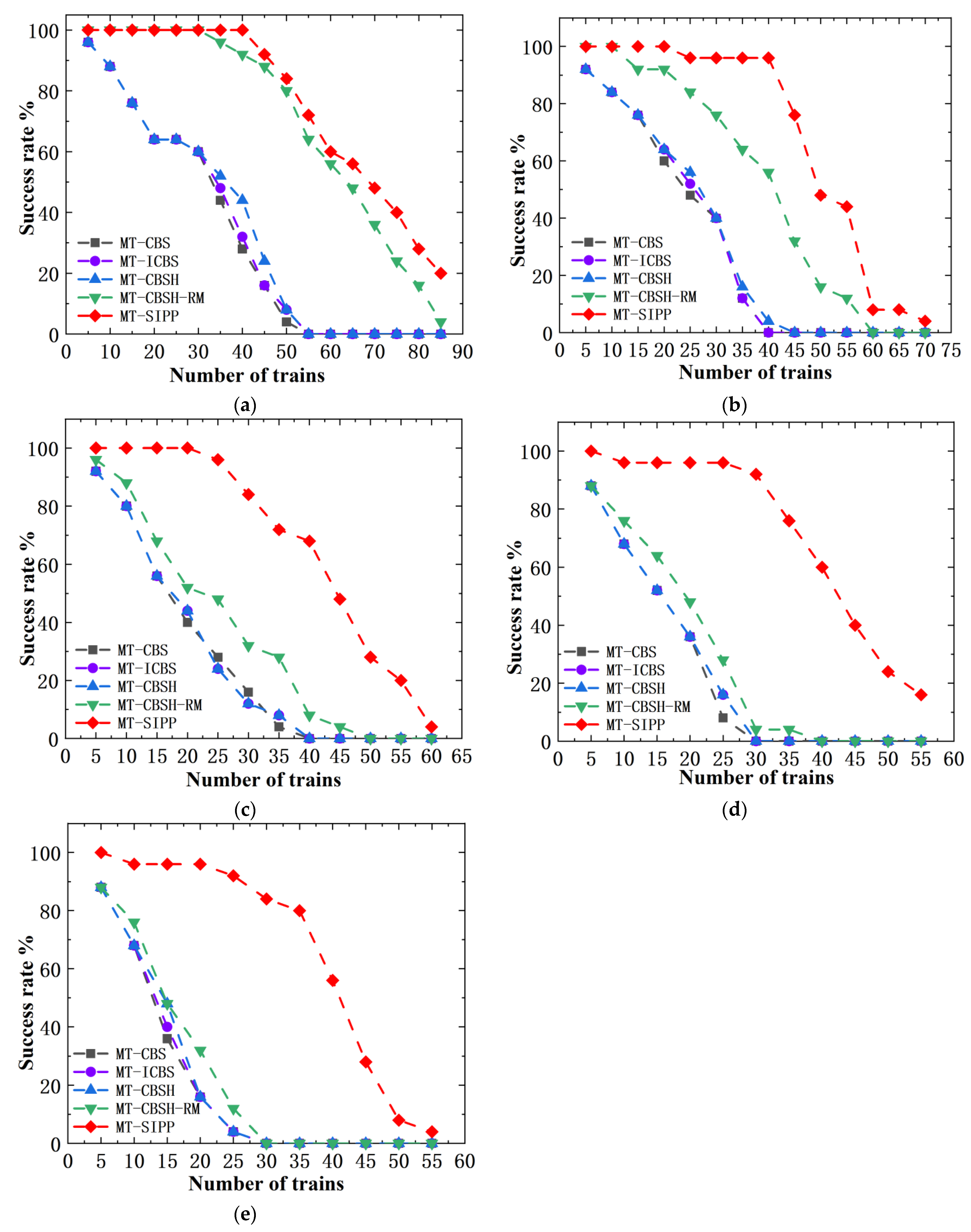
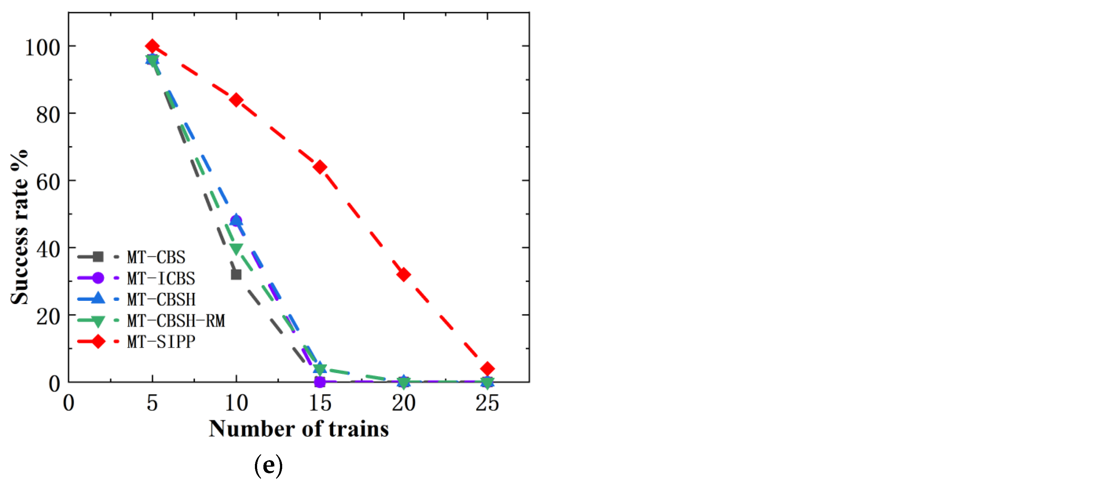
The blank map environment is distinguished by its prominent feature: the entire map space consists of obstacle-free open areas. This environment provides optimal conditions for the unrestricted movement and efficient interaction of multiple robots. As depicted in Figure 12, this study selected this typical blank map environment, sized at 48*48, for evaluating algorithm performance. Figure 13 visually illustrates the comparative results of MT-CBS, MT-ICBS, MT-CBSH, MT-CBSH-RM and MT-SIPP algorithms in terms of their success rates in solving problems within the blank map environment. This comparison offers a clear insight into the performance disparities among the algorithms under these specific environmental conditions.
Based on the success rate comparison depicted in Figure 13, it is evident that among the five multi-train path planning algorithms—MT-CBS, MT-ICBS, MT-CBSH, MT-CBSH-RM and the proposed MT-SIPP algorithm consistently exhibit the highest success rates in the empty map environment. Of particular note is that although the MT-CBSH-RM algorithm, a prominent CBS-type algorithm, shows comparable success rates to the MT-SIPP algorithm when the value of (train body length) is small, the superiority of the MT-SIPP algorithm becomes more pronounced as increases. Detailed statistical analysis reveals that at , the MT-SIPP algorithm exhibited average success rate improvements of 44.7%, 44%, 42.6%, and 5.6% compared to the other four algorithms. At , these enhancements were 40%, 38%, 39%, and 17%. At , the improvements were consistently 42%, 42%, 42%, and 33%. Notably, at , the algorithm achieved substantial improvements of 49.1%, 48.4%, 48.4%, and 43.6%, while at , the figures were 48%, 47.6%, 46.9%, and 44%. These findings underscore a significant performance advantage of the MT-SIPP algorithm over CBS-like multi-agent pathfinding algorithms in achieving higher success rates, with an average improvement nearing 40% in blank map environments. Furthermore, regarding the scalability in handling multiple train instances, particularly at larger values (e.g.,), MT-SIPP demonstrated superior capability, effectively managing nearly twice the maximum train instances compared to alternative algorithms.
Figure 13.
Comparison of success rates of several algorithms in blank map environment. (a) ; (b) ; (c) ; (d) ; (e) .
Figure 13.
Comparison of success rates of several algorithms in blank map environment. (a) ; (b) ; (c) ; (d) ; (e) .
In our statistical analysis of algorithm runtime (as shown in Table 1), we compared the MT-CBSH-RM algorithm, known for its superior efficiency in CBS-like multi-train planning algorithms, with the MT-SIPP algorithm. In a blank map environment, MT-CBSH-RM demonstrates better algorithmic runtime efficiency than MT-SIPP when (train length) is small or when solving a small number of trains. However, as the number of trains or increases, CBS-like multi-train planning algorithms experience rapid expansion of their solution space, resulting in a gradual decline in efficiency. This efficiency gap becomes more pronounced with increasing problem complexity.
The aforementioned results indicate that in a blank map environment, CBS-like multi-train planning algorithms, particularly the MT-CBSH-RM algorithm, excel in both success rate and runtime efficiency when values are small and the number of trains is limited. This is largely attributed to the expansive layout of the map, which allows ample maneuvering space for trains. However, as the number of trains increases or values grow larger, the available maneuvering space for trains gradually diminishes, leading to a significant decrease in the solving efficiency of CBS-like algorithms. In contrast, under these circumstances, the MT-SIPP algorithm consistently maintains higher solving efficiency, demonstrating its superior performance in handling complex multi-train pathfinding problems.

Table 1.
Running time statistics of the two algorithms in blank map environment.
| value | /seconds | |||||
|---|---|---|---|---|---|---|
| MT-SIPP | MT-CBSH-RM | MT-SIPP | MT-CBSH-RM | |||
| =1 | 5 | 0.416 | 0.003 | 45 | 11.073 | 17.743 |
| 10 | 0.563 | 0.007 | 50 | 21.69 | 26.874 | |
| 15 | 0.725 | 0.019 | 55 | 35.186 | 46.069 | |
| 20 | 1.051 | 0.035 | 60 | 48.575 | 46.335 | |
| 25 | 1.548 | 0.053 | 65 | 54.116 | 62.783 | |
| 30 | 1.851 | 0.109 | 70 | 68.208 | 78.754 | |
| 35 | 7.377 | 5.155 | 75 | 79.471 | 92.465 | |
| 40 | 8.529 | 7.244 | 80 | 93.359 | 101.921 | |
| =2 | 5 | 0.432 | 0.016 | 35 | 7.996 | 44.751 |
| 10 | 0.615 | 0.022 | 40 | 9.569 | 64.221 | |
| 15 | 1.103 | 9.75 | 45 | 34.138 | 85.798 | |
| 20 | 1.573 | 9.946 | 50 | 66.568 | 101.118 | |
| 25 | 6.874 | 20.533 | 55 | 72.455 | 105.727 | |
| 30 | 7.495 | 29.742 | ||||
| =3 | 5 | 0.483 | 5.153 | 30 | 22.032 | 81.689 |
| 10 | 0.729 | 16.249 | 35 | 36.948 | 87.988 | |
| 15 | 1.058 | 39.504 | 40 | 42.265 | 110.499 | |
| 20 | 1.474 | 57.664 | 45 | 66.665 | 115.241 | |
| 25 | 6.918 | 62.574 | ||||
| =4 | 5 | 0.443 | 14.934 | 25 | 9.1 | 86.532 |
| 10 | 6.111 | 29.459 | 30 | 14.32 | 115.222 | |
| 15 | 6.541 | 44.933 | 35 | 33.654 | 106.918 | |
| 20 | 7.456 | 62.731 | ||||
| =5 | 5 | 0.663 | 15.201 | 20 | 8.188 | 82.982 |
| 10 | 6.363 | 30.023 | 25 | 14.849 | 106.183 | |
| 15 | 6.664 | 64.845 | ||||
7.2. Random Map Environment Testing
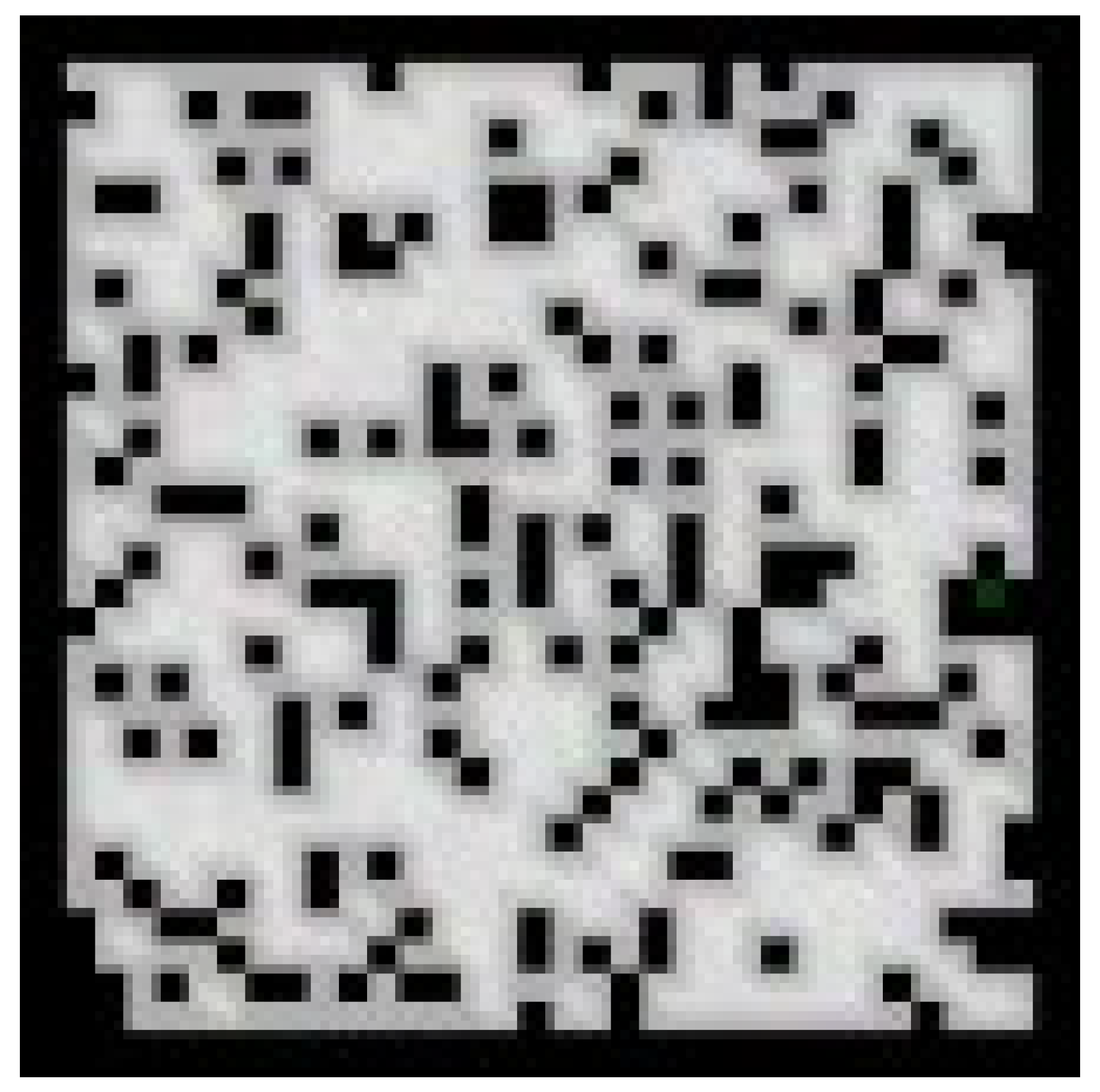
In a random map environment, the distribution of obstacles is stochastic, leading to dispersed and variably-sized passable areas for trains. This variability undoubtedly presents considerable challenges for multi-train planning on such maps. As depicted in Figure 14, this study utilized a representative random map measuring 32*32 for testing purposes. To thoroughly evaluate the performance of diverse algorithms in this setting, comprehensive testing was conducted, and the findings are consolidated in Figure 15 and Table 2.
Figure 14.
Random map random-32-32-20.
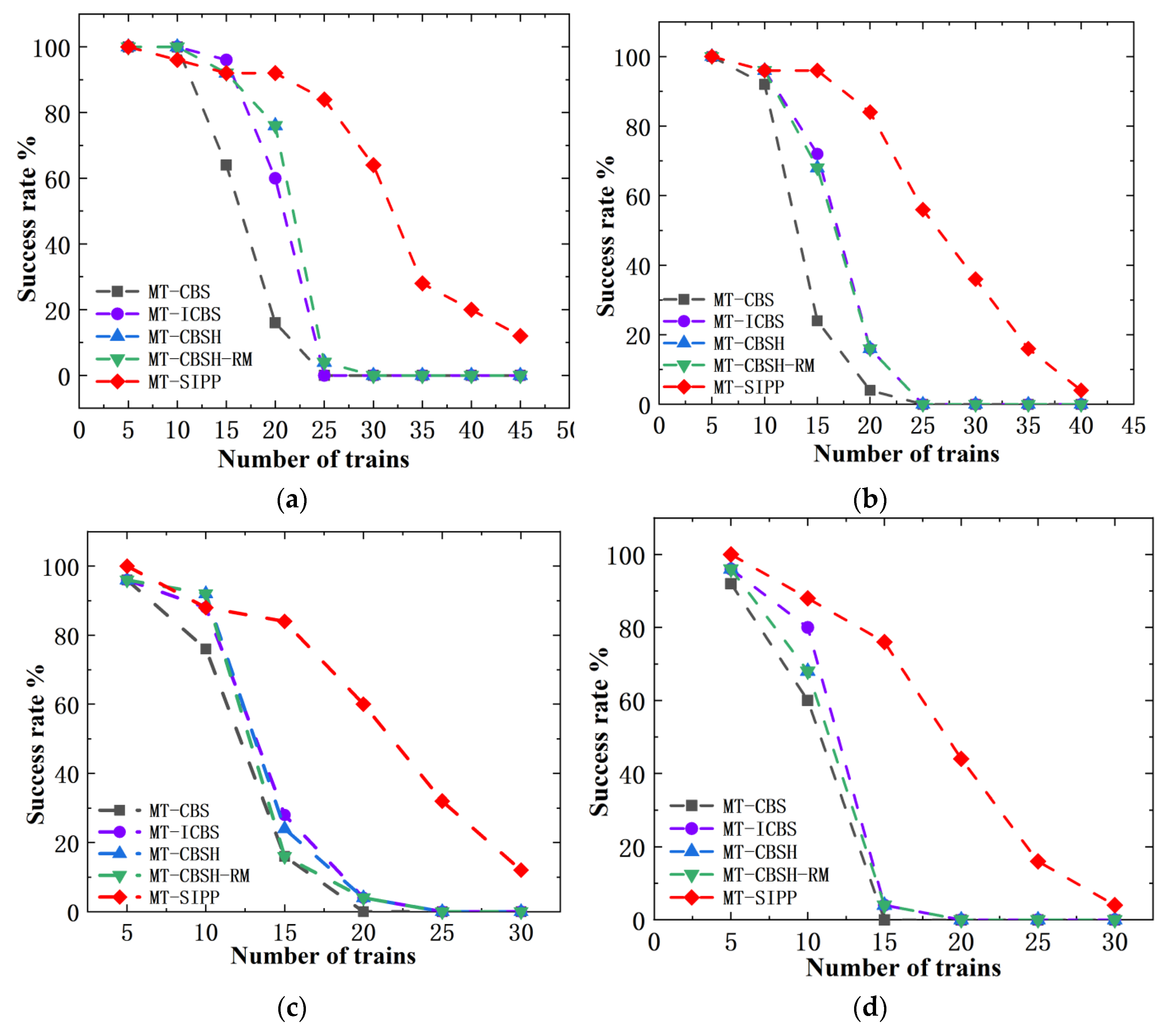
Based on the comparative results of success rates depicted in Figure 15, it is evident that in random map environments, the high coverage of obstacles leads to an increasing number of conflicts among trains as the number of trains to be solved increases. This diminishes the available maneuvering space and gradually lowers the success rates of all algorithms. Furthermore, as the value of (train car length) increases, the number of empty grid occupied by trains and their occupation duration also increase, thereby reducing the maximum feasible number of trains that can be effectively managed by several multi-train planning algorithms. Nevertheless, it is worth noting that across various values, the MT-SIPP algorithm consistently achieves higher success rates than several other algorithms. This superiority is particularly evident at . In contrast, CBS-like multi-train path planning algorithms show minimal differences in success rates, with their performance nearly converging as increases. This trend primarily stems from the constrained passable areas in random maps. At lower values, the enhancement strategies integrated into the MT-CBS algorithm contribute to improved success rates. However, as increases, the further reduction in passable space and the rapid growth in conflict search state space diminish the effectiveness of these strategies in enhancing success rates. Overall, the MT-SIPP algorithm exhibits an average increase in success rates of approximately 30% compared to CBS-like multi-train planning algorithms. Particularly noteworthy is its ability to handle more than twice the maximum number of solvable trains compared to CBS-like algorithms when . This robust performance underscores the superiority of MT-SIPP in addressing multi-train path planning challenges in random map environments.
Figure 15.
Comparison of solving success rates of several algorithms in a random map environment. (a) ; (b) ; (c) ; (d) ; (e) .
Figure 15.
Comparison of solving success rates of several algorithms in a random map environment. (a) ; (b) ; (c) ; (d) ; (e) .
According to the data analysis from Table 2, the prevalence of numerous random obstacles in random map environments significantly complicates the task of multi-train planning. In scenarios with smaller values and fewer trains to solve, the MT-CBSH-RM algorithm indeed exhibits shorter runtimes compared to the MT-SIPP algorithm. However, once the number of trains to be solved exceeds 10, regardless of the value, the runtime of the MT-CBSH-RM algorithm experiences exponential growth, making it difficult to provide solutions within a reasonable time frame.
In contrast, while the MT-SIPP algorithm does experience increased runtime as the number of trains to solve increases, the magnitude of this increase is significantly smaller compared to the MT-CBSH-RM algorithm. Consequently, when solving for more than 10 trains (i.e.,), the MT-SIPP algorithm consistently demonstrates shorter runtimes than MT-CBSH-RM, sometimes averaging as little as one-tenth of the latter's runtime. This finding strongly validates the superior performance of the MT-SIPP algorithm in addressing large-scale multi-train planning problems.
Table 2.
Running time statistics of the two algorithms in random map environment.
| value | /seconds | |||||
|---|---|---|---|---|---|---|
| MT-SIPP | MT-CBSH-RM | MT-SIPP | MT-CBSH-RM | |||
| =1 | 5 | 0.525 | 0.007 | 25 | 20.361 | 35.737 |
| 10 | 0.589 | 0.051 | 30 | 35.097 | 88.66 | |
| 15 | 0.712 | 4.976 | 35 | 44.867 | 109.902 | |
| 20 | 10.062 | 10.319 | 40 | 68.949 | 118.032 | |
| =2 | 5 | 0.586 | 0.011 | 20 | 20.281 | 91.697 |
| 10 | 0.919 | 2.651 | 25 | 30.889 | 107.895 | |
| 15 | 6.104 | 35.48 | 30 | 59.613 | 117.054 | |
| =3 | 5 | 0.597 | 0.043 | 15 | 15.924 | 77.715 |
| 10 | 10.545 | 31.168 | 20 | 31.347 | 108.167 | |
| =4 | 5 | 0.592 | 4.914 | 15 | 31.447 | 115.636 |
| 10 | 10.406 | 56.327 | 20 | |||
| =5 | 5 | 0.594 | 10.639 | 10 | 6.234 | 82.654 |
7.3. Indoor Map Environment Testing
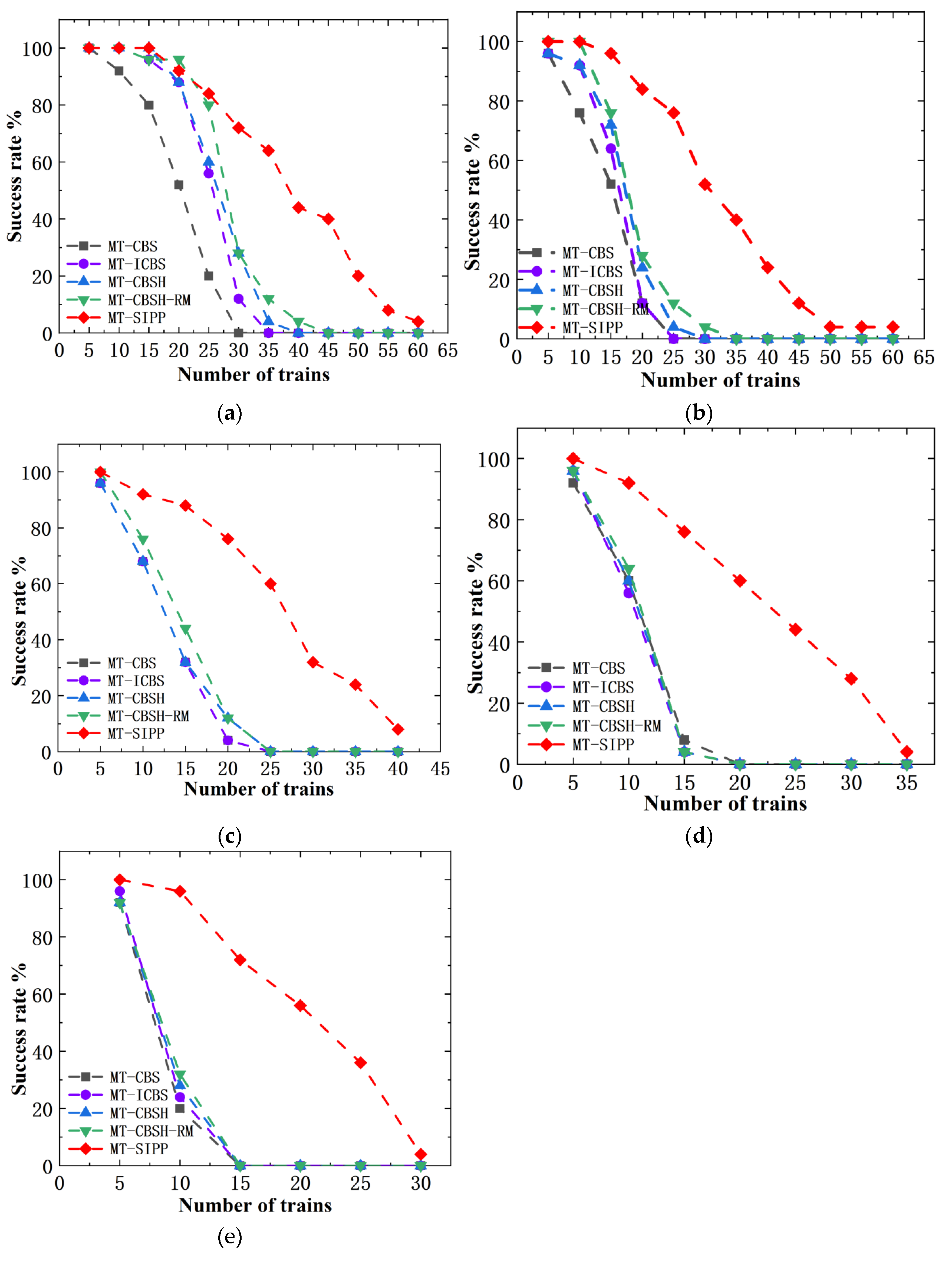
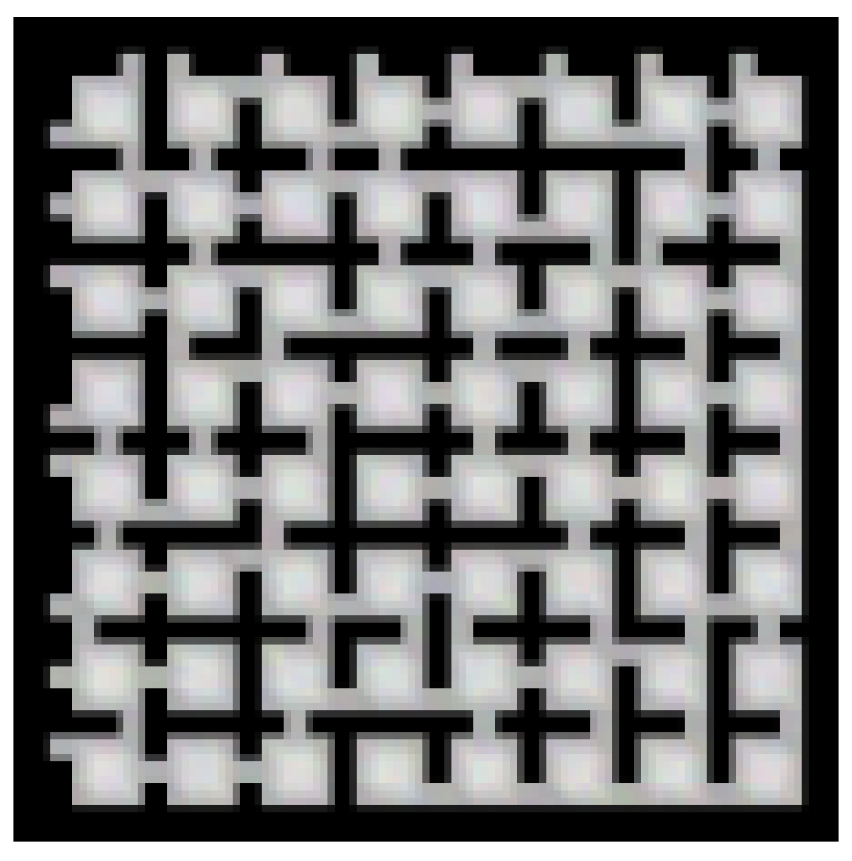
The indoor map environment replicates the layout of partially enclosed rooms typically found in real-world scenarios, interconnected by narrow passages allowing only one train to pass at a time. In this unique map environment, characterized by spatial constraints and restricted passages, congestion between trains can readily occur, thereby greatly augmenting the complexity and challenges associated with multi-train planning. The indoor room map we tested is illustrated in Figure 16, with comprehensive test results detailed in Figure 17 and Table 3.
In Figure 17, we have contrasted the success rates of several algorithms in solving room-based maps. The findings reveal that MT-CBS exhibits the lowest success rate, whereas the MT-SIPP algorithm displays the highest success rate. It is worth noting that the performance of the multi-train path planning algorithms that incorporate improvements over MT-CBS shows varying degrees of success and consistency. In specific terms, at , both the MT-CBSH and MT-CBSH-RM algorithms achieve identical success rates, slightly edging out MT-ICBS. However, as increases, the scenario evolves. At and , MT-ICBS shows slightly superior performance compared to MT-CBSH and MT-CBSH-RM. Conversely, at , MT-CBSH-RM outperforms MT-ICBS and MT-CBSH. By , MT-CBSH exhibits marginally better performance than MT-CBSH-RM and MT-ICBS. This inconsistency in results may be attributed to the unique characteristics of room-based maps and the high complexity inherent in multi-train path planning. In certain cases, the addition of more improvement strategies might inadvertently reduce success rates due to increased algorithmic complexity. Overall, in room-based maps, the MT-SIPP algorithm exhibits a notable average increase of approximately 27% in success rates compared to CBS-like multi-train path planning algorithms. This improvement is quite significant.
Figure 17.
Comparison of the success rates of several algorithms in the room map environment. (a) ; (b) ; (c) ; (d) ; (e) .
Figure 17.
Comparison of the success rates of several algorithms in the room map environment. (a) ; (b) ; (c) ; (d) ; (e) .
Based on the data from Table 3, in the context of room-based map environments, it is observed that when and the number of trains is less than 10, the MT-CBSH-RM algorithm indeed shows shorter runtime compared to the MT-SIPP algorithm. However, across all other test conditions, the MT-SIPP algorithm consistently demonstrates shorter runtime.
It is noteworthy that many of the connecting passages between rooms in the room-based maps are single-channel, significantly restricting the throughput of trains. This structural limitation predisposes CBS-like multi-train planning algorithms to conflict generation when applied in such environments. To find conflict-free solutions, algorithms must continually search and replan numerous potential conflict nodes, which inevitably consumes substantial computational resources. Particularly in densely populated train scenarios, achieving a conflict-free solution becomes increasingly challenging. Therefore, the MT-SIPP algorithm demonstrates superior efficiency and adaptability in tackling these intricate indoor multi-train planning problems.
Table 3.
Running time statistics of the two algorithms in room map environment.
| value | /seconds | |||||
|---|---|---|---|---|---|---|
| MT-SIPP | MT-CBSH-RM | MT-SIPP | MT-CBSH-RM | |||
| =1 | 5 | 0.141 | 0.003 | 20 | 10.313 | 45.438 |
| 10 | 5.043 | 0.048 | 25 | 20.793 | 118.389 | |
| 15 | 9.918 | 11.623 | ||||
| =2 | 5 | 0.182 | 1.978 | 15 | 5.499 | 45.446 |
| 10 | 4.282 | 5.012 | 20 | 20.964 | 102.241 | |
| =3 | 5 | 0.206 | 4.825 | 15 | 21.503 | 103.262 |
| 10 | 15.235 | 11.454 | 20 | 50.649 | 115.955 | |
| =4 | 5 | 0.201 | 4.835 | 15 | 31.383 | 115.334 |
| 10 | 15.659 | 46.146 | ||||
| =5 | 5 | 0.197 | 5.028 | 15 | 45.167 | 117.688 |
| 10 | 20.641 | 75.108 | ||||
7.4. Analysis and Discussion of Experimental Results
The experimental results across various map environments indicate that while strategies such as integrating heuristic function -value guidance in search and employing MDD for rectangle conflict resolution can enhance the solving capabilities of the MT-CBS algorithm to some extent, its effectiveness is hindered by the CBS algorithm's reliance on unit discretization nodes for path expansion and conflict detection mechanisms. This limitation results in an exponential increase in solution space as the number of trains and train lengths grow. Despite the incorporation of additional improvement strategies, the overall enhancement in algorithmic efficiency remains rather limited. In contrast, the MT-SIPP algorithm proposed in this study primarily expands path nodes and avoids conflicts based on global safe intervals, demonstrating a linear relationship between search space and both and . Consequently, as and increase beyond certain thresholds, the superior efficiency of the MT-SIPP algorithm in solution space becomes increasingly apparent.
All test results unequivocally demonstrate that our algorithm surpasses existing multi-train path planning algorithms in several key metrics: success rate, maximum number of solvable trains, and algorithm runtime. Particularly notable is the MT-SIPP algorithm's ability to achieve shorter runtimes and higher solving efficiency when confronted with larger numbers of trains and longer train lengths . Furthermore, our algorithm guarantees that the total cost of generated path solutions deviates from the optimal path's total cost by no more than 10%. In scenarios involving blank maps or random and room-based maps with fewer trains, this deviation is further minimized to within 5%. This thoroughly validates the feasibility and efficacy of our algorithm. Despite making compromises in total path cost, its significant advancements in success rate, maximum solvable capacity, and solving efficiency underscore its broad applicability in the realm of multi-train path planning.
8. Conclusions
To achieve cost savings and improve transport efficiency, snake-like robots, akin to train-like transport vehicles, are widely employed across multiple scenarios for cargo handling operations. However, in CBS-like multi-train path planning algorithms, the detection and resolution of conflicts for each segment of a snake-like robot occupying grid nodes often entail intricate processes of conflict node splitting and path searching. This significantly increases the algorithm's runtime. At times, such complexity may prevent the algorithm from delivering feasible solutions within the allocated time, thereby failing to meet the efficient path planning requirements of multi-robot systems.
In addressing this challenge, we propose the Multi-Train Safety Interval Path Planning (MT-SIPP) algorithm in this study. This algorithm harnesses the benefits of safety intervals in solving path planning issues for snake-like robots. By directly adjusting safety intervals and incorporating additional node constraints, it efficiently mitigates conflicts among snake-like robots, thereby markedly improving path planning efficiency. The simulation test results convincingly validate the superiority of the MT-SIPP algorithm. Compared to MT-CBS, MT-ICBS, MT-CBSH, and MT-CBSH-RM algorithms, MT-SIPP demonstrates significant advancements in both solving capability and efficiency. Specifically, our algorithm shows an average 28% increase in success rate and can handle up to twice the maximum number of trains solvable by other algorithms. Particularly in scenarios with a large number of trains and longer train lengths, MT-SIPP consistently provides solutions rapidly and efficiently, thereby demonstrating its exceptional performance in the field of multi-train path planning.
Author Contributions
Conceptualisation, Jinchao Miao; Formal Analysis, Ping Li and Liwei Yang; Financing Acquisitions, Liwei Yang; Methodology, Jinchao Miao and Ping Li; Resources, Ping Li; Writing - Raw Drafts, Jinchao Miao; Writing - Review and Editing, Ping Li and Liwei Yang. All authors have read and agreed to the published version of the manuscript.
Funding
This work was supported by “Scientific Research Project on Basic Research Operating Expenses of Universities in the Autonomous Region (XJEDU2024P090)”.
Conflicts of Interest
The authors declare no conflicts of interest.
Data availability statements
The original contributions presented in the study are included in the article/supplementary material, further inquiries can be directed to the corresponding author/s.
References
- Chen, X.; Li, Y.; Liu, L. A coordinated path planning algorithm for multi-robot in intelligent warehouse. In Proceedings of the International Conference on Robotics and Biomimetics; IEEE: USA, 2019; pp. 2945–2950. [Google Scholar]
- Ma, H.; Hönig, W.; Kumar, T.K.S.; et al. Lifelong path planning with kinematic constraints for multi-agent pickup and delivery. In Proceedings of the AAAI Conference on Artificial Intelligence; AAAI Press: USA, 2019; Volume 33, pp. 7651–7658. [Google Scholar]
- Furchì, A.; Lippi, M.; Carpio, R.F.; et al. Route optimization in precision agriculture settings: a multi-steiner TSP formulation. IEEE Transactions on Automation Science and Engineering 2022. [Google Scholar] [CrossRef]
- Han, S.D.; Yu, J. Effective heuristics for multi-robot path planning in warehouse environments. In Proceedings of the 2019 International Symposium on Multi-Robot and Multi-Agent Systems (MRS); IEEE: USA, 2019; pp. 10–12. [Google Scholar]
- Chen, X.; Li, Y.; Liu, L. A coordinated path planning algorithm for multi-robot in intelligent warehouse. In Proceedings of the 2019 IEEE International Conference on Robotics and Biomimetics (ROBIO); IEEE: USA, 2019; pp. 2945–2950. [Google Scholar]
- Stern, R.; Sturtevant, N.; Felner, A.; et al. Multi-agent pathfinding: Definitions, variants, and benchmarks. In Proceedings of the International Symposium on Combinatorial Search; AAAI Press: USA, 2019; Volume 10, pp. 151–158. [Google Scholar]
- Ma, H.; Kumar, T.K.S.; Koenig, S. Multi-agent path finding with delay probabilities. In Proceedings of the AAAI Conference on Artificial Intelligence; AAAI Press: USA, 2017; Volume 31. [Google Scholar]
- Hönig, W.; Kiesel, S.; Tinka, A.; et al. Persistent and robust execution of MAPF schedules in warehouses. IEEE Robotics and Automation Letters 2019, 4, 1125–1131. [Google Scholar] [CrossRef]
- Li, B.; Page, B.R.; Moridian, B.; et al. Collaborative mission planning for long-term operation considering energy limitations. IEEE Robotics and Automation Letters 2020, 5, 4751–4758. [Google Scholar] [CrossRef]
- Cohen, L.; Uras, T.; Kumar, T.K.; et al. Optimal and bounded-suboptimal multi-agent motion planning. In Proceedings of the International Symposium on Combinatorial Search; AAAI Press: USA, 2019; Volume 10, pp. 44–51. [Google Scholar]
- Li, J.; Chen, Z.; Harabor, D.; et al. MAPF-LNS2: Fast repairing for multi-agent path finding via large neighborhood search. In Proceedings of the AAAI Conference on Artificial Intelligence; AAAI Press: USA, 2022; Volume 36, pp. 10256–10265. [Google Scholar]
- Li, B.; Ma, H. Double-deck multi-agent pickup and delivery: Multi-robot rearrangement in large-scale warehouses. IEEE Robotics and Automation Letters 2023. [Google Scholar] [CrossRef]
- Sharon, G.; Stern, R.; Felner, A.; et al. Conflict-based search for optimal multi-agent pathfinding. Artificial Intelligence 2015, 219, 40–66. [Google Scholar] [CrossRef]
- Boyarski, E.; Felner, A.; Stern, R.; et al. ICBS: The improved conflict-based search algorithm for multi-agent path finding. In Proceedings of the 8th International Symposium on Combinatorial Search; AAAI Press: USA, 2015; pp. 223–225. [Google Scholar]
- Felner, A.; Li, J.; Boyarski, E.; et al. Adding heuristics to conflict-based search for multi-agent path finding. In Proceedings of the 28th International Conference on Automated Planning and Scheduling; AAAI Press: Menlo Park, USA, 2018; pp. 83–87. [Google Scholar]
- Li, J.; Harabor, D.; Stuckey, P.J.; et al. Symmetry-breaking constraints for grid-based multi-agent path finding. In Proceedings of the AAAI Conference on Artificial Intelligence; AAAI Press: USA, 2019; Volume 33, pp. 6087–6095. [Google Scholar]
- Atzmon, D.; Stern, R.; Felner, A.; et al. Robust multi-agent path finding. In Proceedings of the International Symposium on Combinatorial Search; AAAI Press: USA, 2018; Volume 9, pp. 2–9. [Google Scholar]
- Phillips, M.; Likhachev, M. Sipp: Safe interval path planning for dynamic environments. In Proceedings of the 2011 IEEE international conference on robotics and automation; IEEE: USA, 2011; pp. 5628–5635. [Google Scholar]
- Yakovlev, K.; Andreychuk, A.; Stern, R. Revisiting bounded-suboptimal safe interval path planning. In Proceedings of the International Conference on Automated Planning and Scheduling; AAAI Press: USA, 2020; Volume 30, pp. 300–304. [Google Scholar]
- Takemori, T.; Tanaka, M.; Matsuno, F. Gait design for a snake robot by connecting curve segments and experimental demonstration. IEEE Transactions on Robotics 2018, 34, 1384–1391. [Google Scholar] [CrossRef]
- Laurent, F.; Schneider, M.; Scheller, C.; et al. Flatland competition 2020: MAPF and MARL for efficient train coordination on a grid world. In Proceedings of the NeurIPS 2020 Competition and Demonstration Track; PMLR: USA, 2021; pp. 275–301. [Google Scholar]
- Lusby, R.M.; Larsen, J.; Ehrgott, M.; et al. Railway track allocation: models and methods. OR spectrum 2011, 33, 843–883. [Google Scholar] [CrossRef]
- Atzmon, D.; Diei, A.; Rave, D. Multi-train path finding. In Proceedings of the International Symposium on Combinatorial SearchA; AAAI Press: USA, 2019; Volume 10, pp. 125–129. [Google Scholar]
- Chen, Z.; Li, J.; Harabor, D.; et al. Multi-Train Path Finding Revisited. In Proceedings of the International Symposium on Combinatorial Search; AAAI Press: USA, 2022; Volume 15, pp. 38–46. [Google Scholar]
- Lan, X.; Lv, X.; Liu, W.; et al. Research on robot global path planning based on improved A-star ant colony algorithm. In Proceedings of the 2021 IEEE 5th Advanced Information Technology, Electronic and Automation Control Conference (IAEAC); IEEE: USA, 2021; Volume 5, pp. 613–617. [Google Scholar]
Figure 1.
Diagram of conflicts. (a) point conflict; (b) edge conflict.
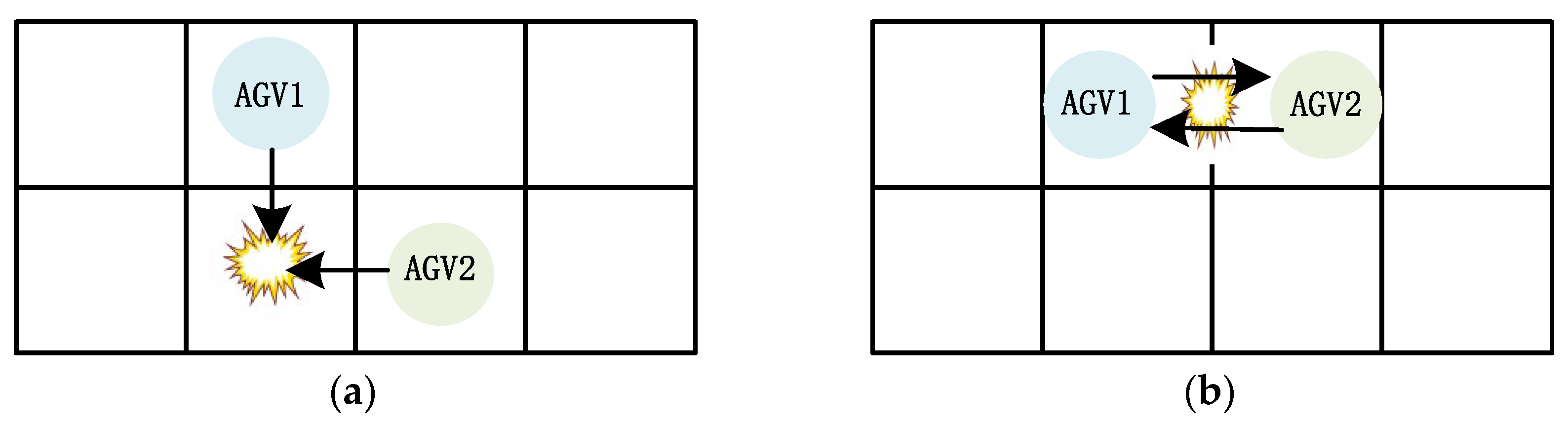
Figure 2.
Point conflict of multi-train robot.
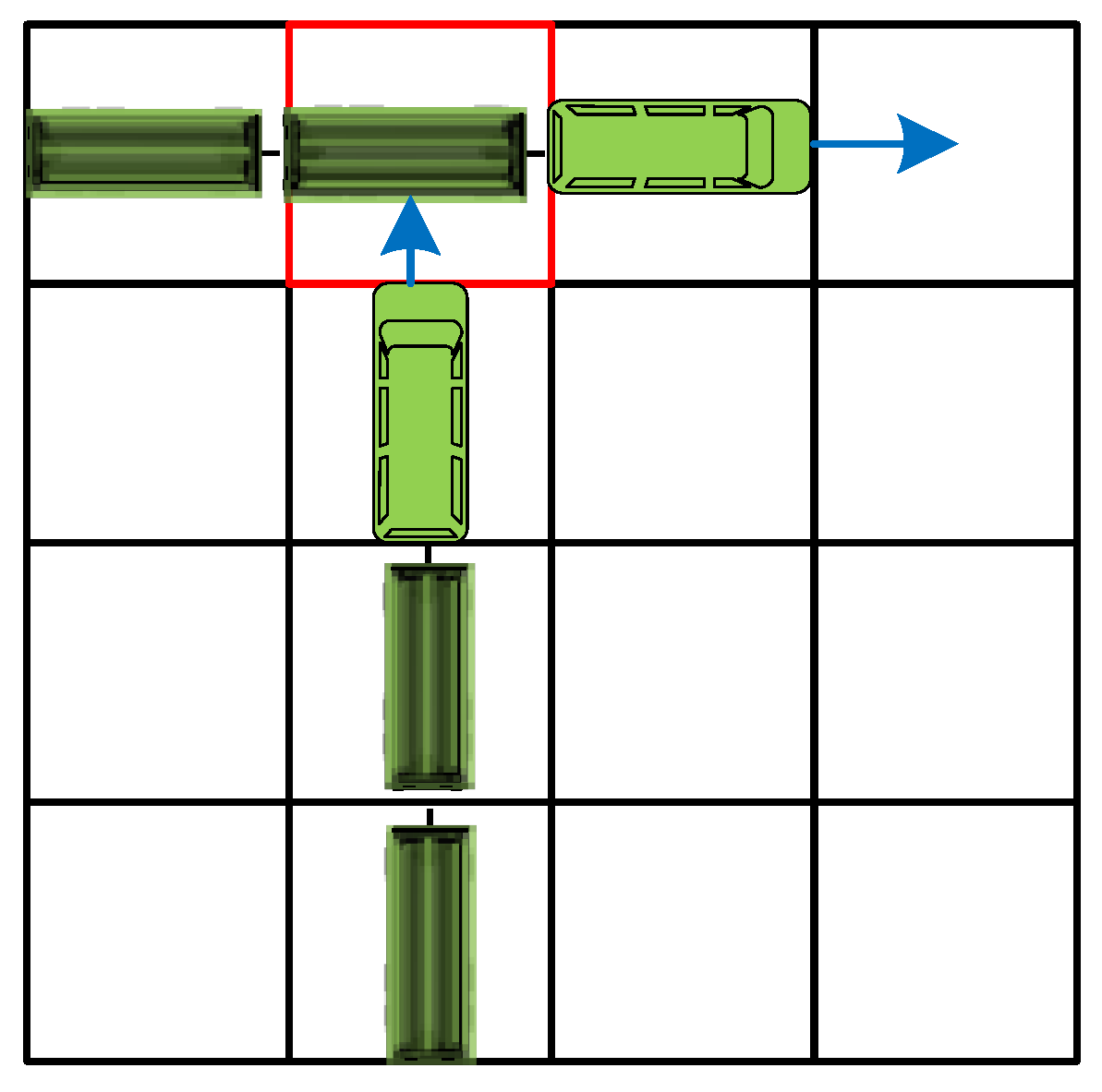
Figure 3.
Schematic of grid security interval update.
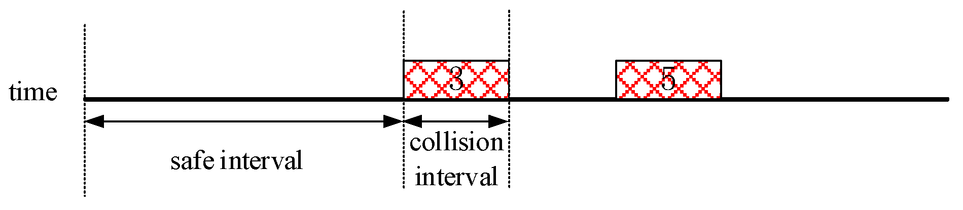
Figure 4.
Grid safety interval update under k robust planning ().
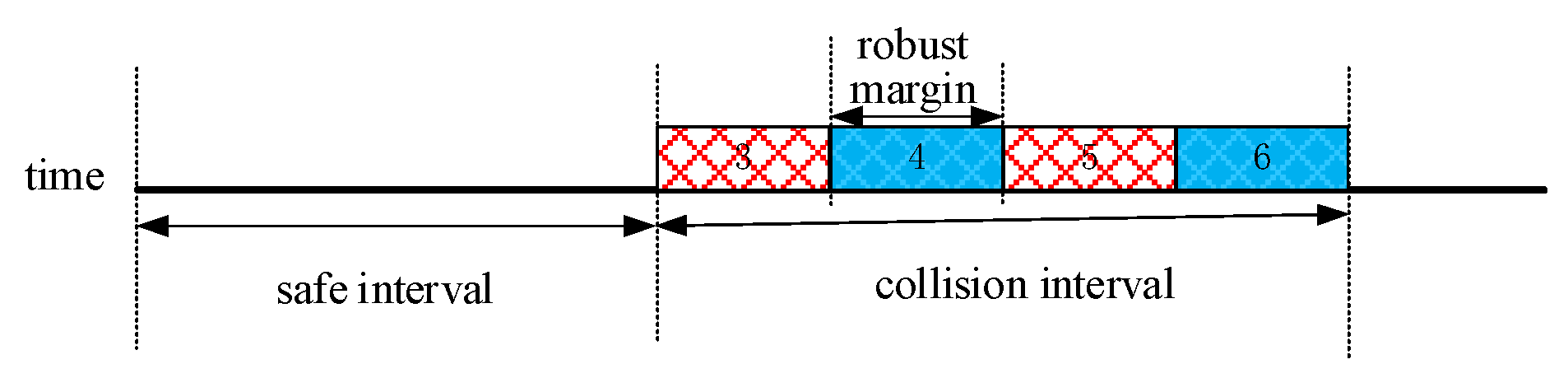
Figure 9.
Three situations in which train stop conflicts occur. (a) Status 1; (b) Status 2; (c) Status 3.
Figure 9.
Three situations in which train stop conflicts occur. (a) Status 1; (b) Status 2; (c) Status 3.
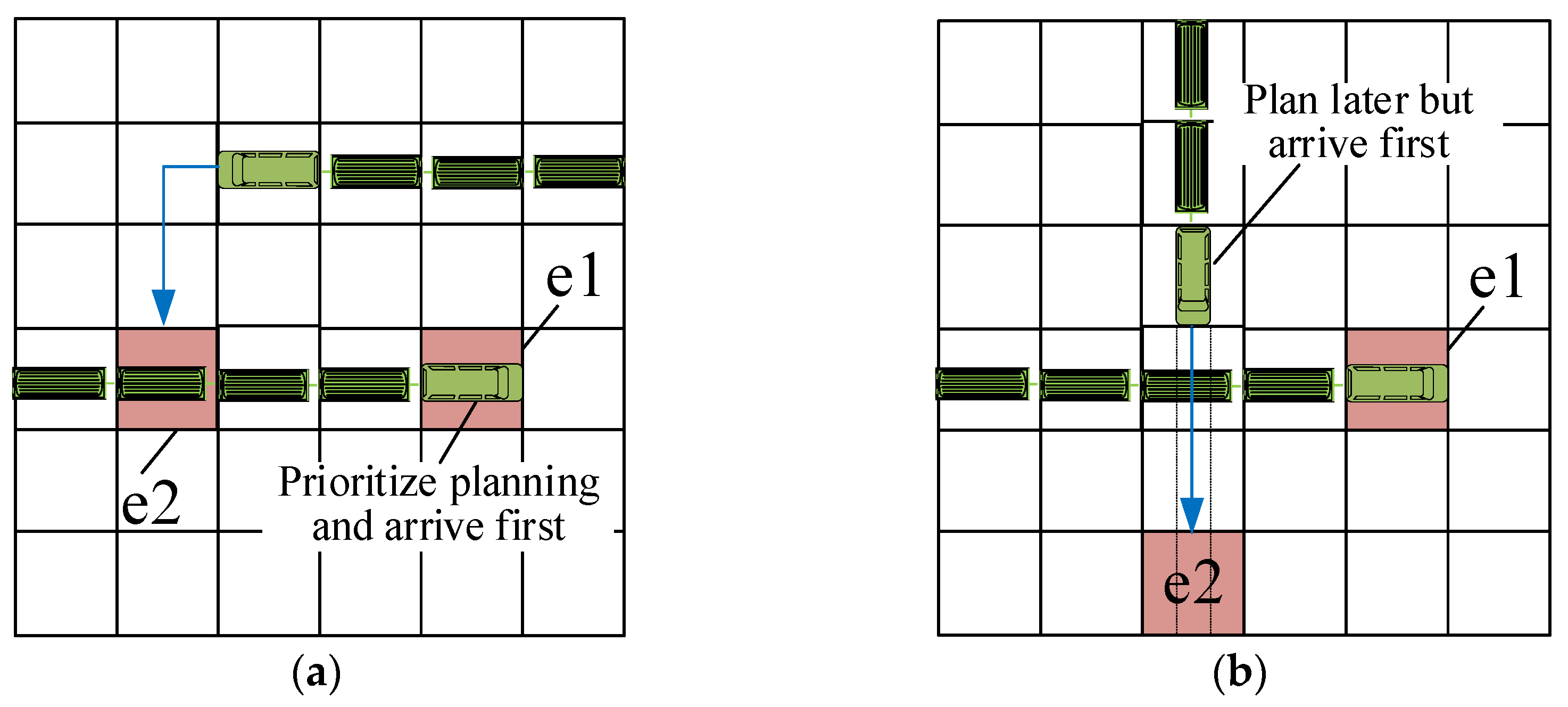
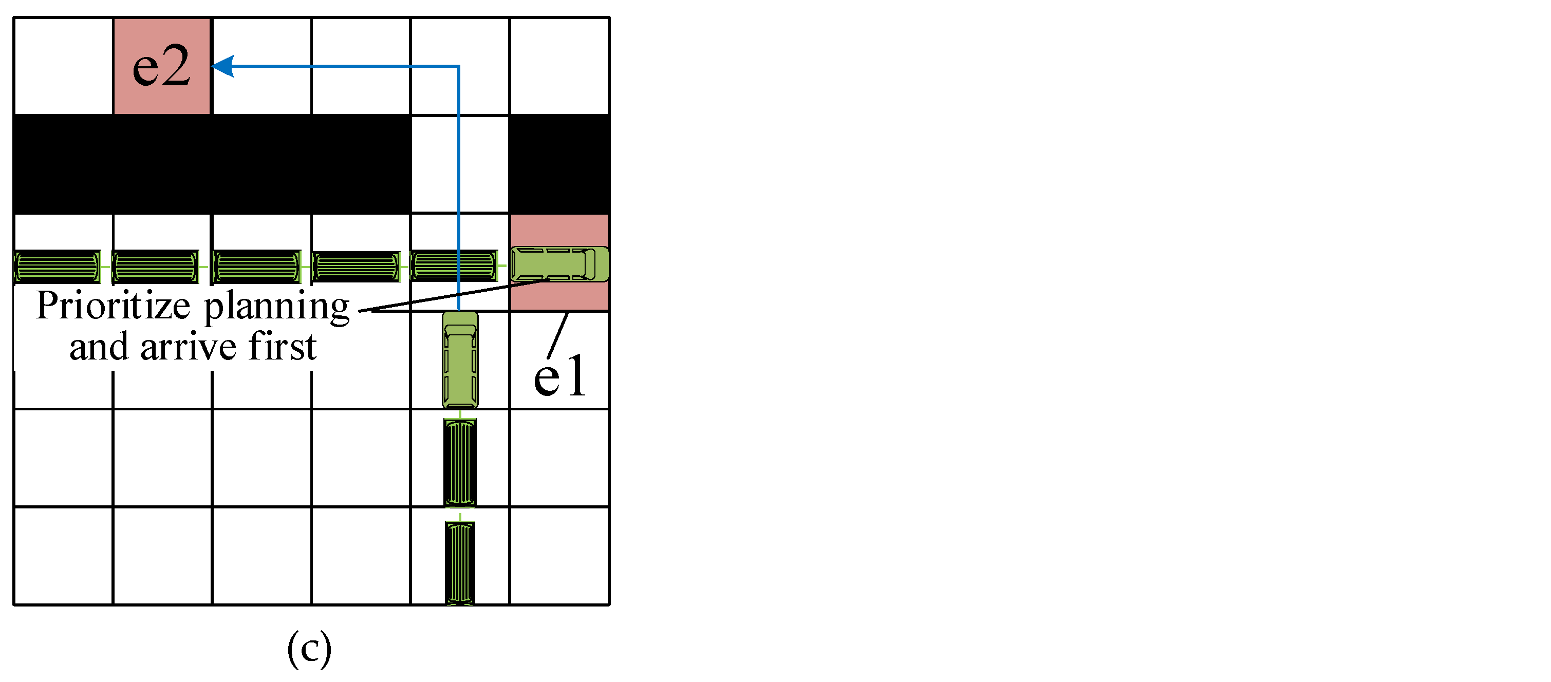
Figure 10.
Update of the safety interval of the car body occupying the grid after the train stops.
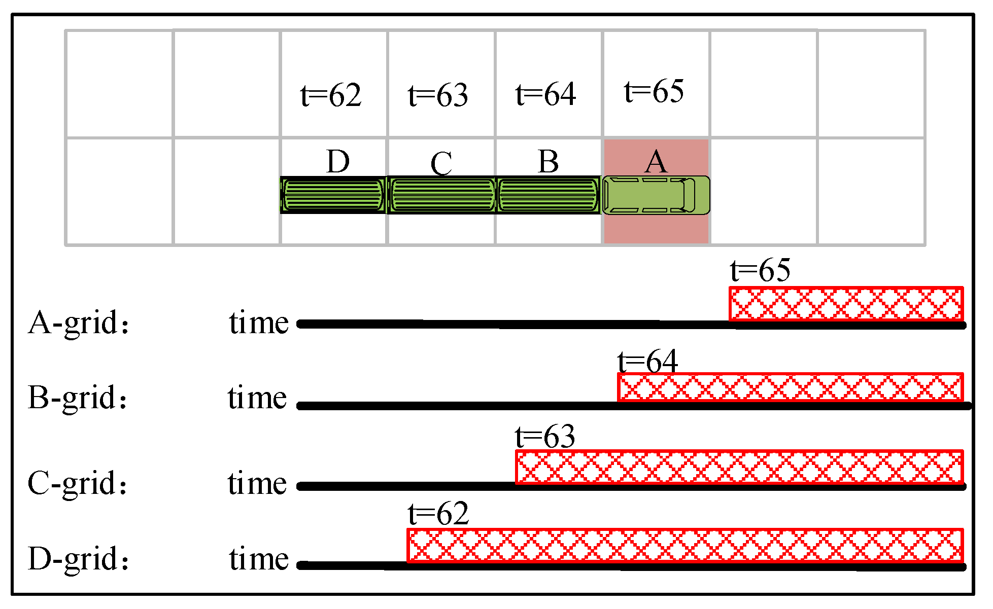
Figure 11.
MT-SIPP algorithm block diagram.
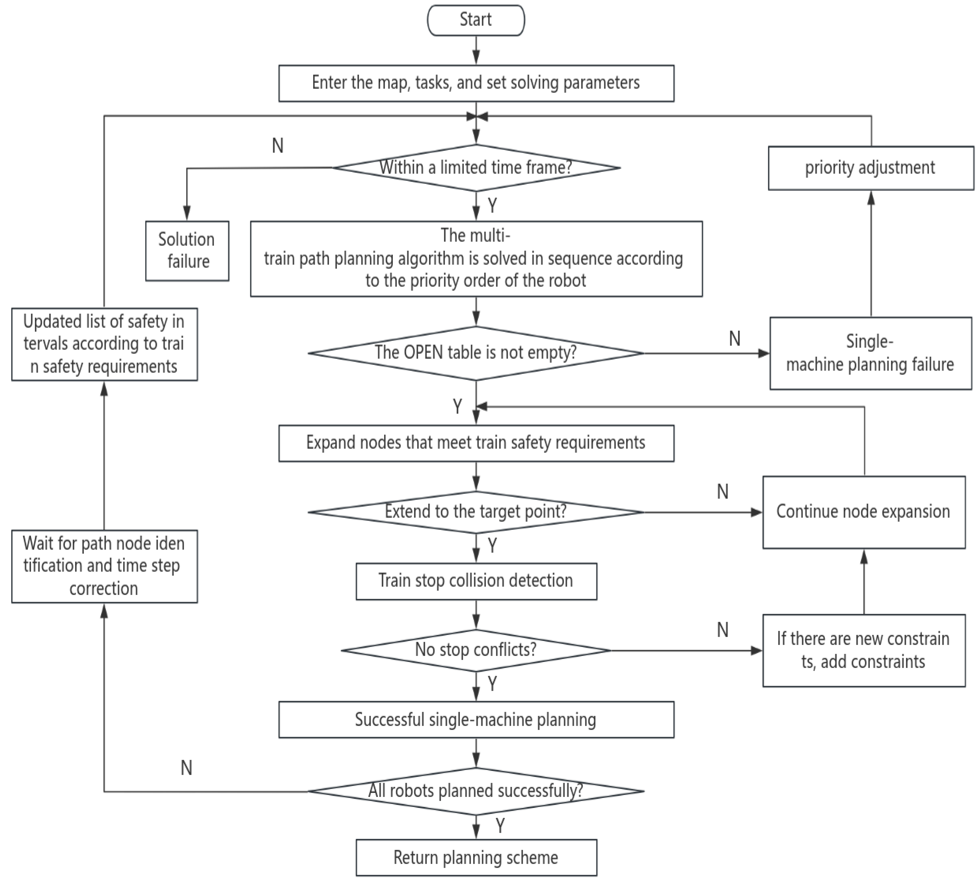
Figure 12.
Empty map Empty-48-48.

Figure 16.
Room map Room-32-32-4.
Disclaimer/Publisher’s Note: The statements, opinions and data contained in all publications are solely those of the individual author(s) and contributor(s) and not of MDPI and/or the editor(s). MDPI and/or the editor(s) disclaim responsibility for any injury to people or property resulting from any ideas, methods, instructions or products referred to in the content. |
© 2024 by the authors. Licensee MDPI, Basel, Switzerland. This article is an open access article distributed under the terms and conditions of the Creative Commons Attribution (CC BY) license (http://creativecommons.org/licenses/by/4.0/).
Copyright: This open access article is published under a Creative Commons CC BY 4.0 license, which permit the free download, distribution, and reuse, provided that the author and preprint are cited in any reuse.


