TransNeural: An Enhanced-Transformer based Performance Pre-Validation Model for Split Learning Tasks

Guangyi Liu; Mancong Kang; Yanhong Zhu; Qingbi Zheng; Maosheng Zhu; Na Li

doi:10.20944/preprints202406.1769.v1

Preprint

Article

TransNeural: An Enhanced-Transformer based Performance Pre-Validation Model for Split Learning Tasks

This version is not peer-reviewed.

Guangyi Liu,

Mancong Kang^*,

Yanhong Zhu^*,Qingbi Zheng,Maosheng Zhu,Na Li

Guangyi Liu,

Mancong Kang^*,

Yanhong Zhu^*,Qingbi Zheng,Maosheng Zhu,Na Li

This version is not peer-reviewed.

Downloads

Views

Comments

Submitted:

25 June 2024

Posted:

25 June 2024

You are already at the latest version

A peer-reviewed article of this preprint also exists.

Abstract

As split learning (SL) becomes popular for addressing data privacy and resource limitation issues in edge model training process, it is crucial to pre-validate whether the extensive use of wireless and computing resources in SL can achieve the expected training latency and convergence. While digital twin network (DTN) can potentially estimate network strategy performance in pre-validation environments, they are still in their infancy for SL tasks, facing challenges like unknown non-i.i.d. data distributions, inaccurate channel states, and misreport resource availability across devices. To address these challenges, this paper proposes a TransNeural algorithm for DTN pre-validation environment to estimate SL latency and convergence. First, the TransNeural algorithm integrates transformers to efficiently model data similarities between different devices, considering different data distributions and device participate sequence greatly influence SL training convergence. Second, it leverages neural network to automatically establish the complex relationships between SL latency and convergence with data distributions, wireless and computing resources, dataset sizes, and training iterations. Deviations in user reports are also accounted for in the estimation process. Simulations show that the TransNeural algorithm improves latency estimation accuracy by 13.44% and convergence estimation accuracy by 116.74% compared to traditional equation-based methods.

Keywords:

;

digital twin network

;

transformer

;

split learning

;

pre-validation environment

Subject:

Engineering - Telecommunications

1. Introduction

In the era of the 6th generation mobile network (6G), an increasing number of artificial intelligence (AI) applications will rely on edge network to train their continually expanding models based on massive amounts of user data [1]. While users may be willing to provide their data with payment, they are concerned about data privacy issues. Meanwhile, fully training AI models on user devices to upload only model parameters can address privacy issues but is often impractical due to constraint user resource [2]. Additionally, companies are reluctant to fully disclose their model parameters, since these are valuable assets [3]. In this context, split learning (SL) has emerged as a promising solution [4]. In SL, an edge server (ES) connected with an access point (AP) offloads only a few lower layers of AI models to a user device for local training, where the device interacts intermediate results in forward and backward propagations with ES to update the upper layers. Once a user device finishes updating using its own data, it sends the updated lower layers to the next user device via AP, continuing this process until all participants have contributed their data. This method protects user privacy and conserves device resources.

With the adoption of SL technology, a crucial concern for AI application companies is to pre-estimate SL latency and convergence performance under given resource allocation strategy before paying users and operators for data, wireless, and computing resources [4]. However, under unknown non-i.i.d. data distribution [5], inaccurate wireless channel state information (CSI), and misreported available computing resources on different user devices, it becomes extremely difficult to accurately estimate the SL performance before real physical executions. The reason is as follows. Suppose there are three participate user devices: A, B, and C. If the data distribution on A is similar to that on C but significantly different from B, then the training sequences A-C-B and A-B-C will result in considerable differences in SL training convergence despite utilizing the same amount of resources. The situation becomes even more problematic when there exists reporting deviations in CSI, amount of data and computing resources on devices. Consequently, AI application companies face high risks when investing heavily in network operators and user devices for SL training on edge, without confidence in achieving their training latency and convergence goals, which significantly dampens their enthusiasm.

Digital Twin Network (DTN), emerging as a critical 6G technology [6], is an intelligent digital replica of a physical network that synchronizes physical states in real-time and uses AI models to analyze the characteristics and relationships of network components for accurate inferences in 6G network [7]. In the context of SL, DTN is expected to automatically model data similarities between devices, account for user misreporting and correct inaccurate CSI based on the unique profiles of different devices. Moreover, it can learn the complex relationships between service performance and network parameters. These functions can be realized based on AI models and form a pre-validation environment in DTN for testing SL strategy performance. Based on the pre-validation results, DTN can repeatedly optimize the SL strategy until it meets latency and convergence requirements before deployment in the physical world.

Nevertheless, several challenges exist in establishing DTN pre-validation environment for SL training tasks. First, learning data similarities between different physical devices is difficult due to data privacy issues, which prevent the acquisition and analysis of user data. Second, accurately estimating the misreported behaviors of each physical device is challenging. These deviations depend on multiple factors such as device version, user behavior, and movement patterns, etc. However, the actual physical information is unattainable due to user privacy, data collection errors, and other factors, making it impossible to learn errors from historical data. Third, it is difficult to model the complex relationships between various SL training performance metrics and network factors like data similarities, dataset size, training iterations, device resources, wireless channel quality, and edge server resources, particularly when there exists unknown parameters. Fourth, the model needs to be broadly applicable to various SL requirements (such as latency, convergence, and energy efficiency) and different tasks. This would enable an autonomous modeling process for pre-validation environments, advancing toward the ultimate goal of realizing fully automatic network management in DTNs [8].

Existing AI models for DTN pre-validation environment can be divided into three categories. First, long short-term memory (LSTM) network are used to establish DTN models for predicting future states. For example, authors in [9] used LSTM to build a network traffic prediction model for DTN based on historical traffic data from a real physical network, which can be utilized for network optimization. Similarly, authors in [10] employed LSTM to model and predict changes in reference signal receiving power, aiming to reduce handover failures in DTN. Second, graph neural network (GNNs) are used to model network topology for strategy pre-validation. For instance, authors in [11] designed a GNN-based pre-validation environment for DTN to estimate delay and jitter under given queuing and routing strategies. Likewise, authors in [12] proposed a GNN-based pre-validation model to estimate end-to-end latencies for different network slicing schemes. Third, a combination of GNN and transformer models is used to capture both temporal and spatial relationships among network components. For example, authors in [13] developed a DTN pre-validation environment that predicts end-to-end quality of service for resource allocation strategies in cloud-native micro-service architectures.

Although existing methods are important explorations for building intelligent DTN pre-validation environment, several problems persist in the context of SL training tasks. First, LSTM is specialized for time-series prediction but not for extracting inter-node relationships, which are crucial for SL training tasks. Second, GNN-based modeling requires pre-known edge relationships to derive network performance. However, inter-node relationships in wireless network are often unknown and complex, considering data similarities and other factors, necessitating an automatic edge construction method. Third, while transformer-based models excel in learning inter-node relationships, they may struggle with understanding the relationships within the feature vector of a single node. This capability is vital for accurately modeling and predicting the performance of SL training tasks in wireless network.

Based on these considerations, this paper presents a TransNeural algorithm for DTN pre-validating environment towards SL training tasks. This algorithm integrates transformers with neural network, leveraging the transformer’s strength in inter-node learning [14] to capture data similarities among different user devices and the neural network’s strength in inter-feature learning [15] to understand the complex relationships between various system variables, SL training performances, and deviation characteristics between different nodes. The contributions of this work can be summarized as follows:

A mathematical model for SL training latency and convergence is established, which jointly considers unknown non-i.i.d. data distributions, device participate sequence, inaccurate CSI, and deviations in occupied computing resources. These are crucial factors for SL training performance but are often overlooked in existing SL studies.
To close the gap in SL-target DTN pre-validation environment, we propose a TransNeural algorithm to estimate SL training latency and convergence under given resource allocation strategies. This algorithm combines the transformer and neural network to model data similarities between devices, establish complex relationships between SL performance and network factors such as data distributions, wireless and computing resources, dataset sizes, and training iterations, and learn the reporting deviation characteristics of different devices.
Simulations show that the proposed TransNeural algorithm improves latency estimation accuracy by $13.44 %$ compared to traditional equation-based algorithms and enhances convergence estimation accuracy by $116.74 %$ .

The remainder of our work is organized as follows. Section 2 gives the system model. Section 3 designs the TransNeural algorithm in DTN for estimating the latency and convergence of SL training tasks. Simulation results and discussions are given in Section 4. Finally, we conclude this paper in Section 5.

2. System Description

In this section, we sequentially present the system model, communication model, SL process and DTN.

2.1. System Model

In our system, there are N user devices access to an AP equipped with an edge server (ES). Each device is charicterized by some unique features including data distributions, the amount of available computing resources, misreporting behaviors, etc. On the n-th device, the dataset is denoted as

Q_{n}

with total size

Q_{n}^{sum} = | | Q_{n} | |

; the amount of available computing resource is denoted as

f_{n}

. The data similarities between different devices depend on their users habits (such as shopping habits) and behaviors. The distance between the n-th device with AP is denoted as d.

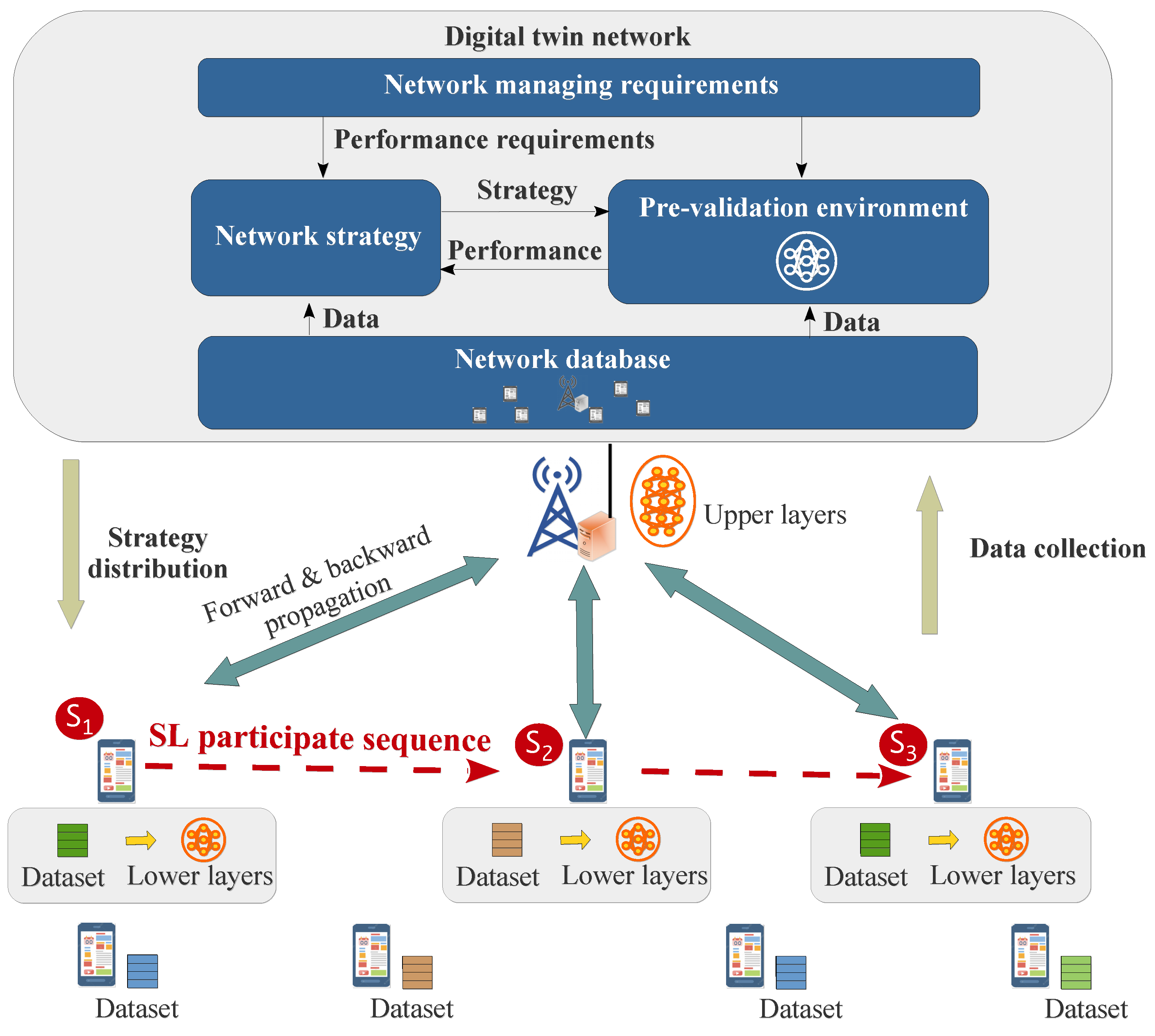
There is a DTN deployed on the ES, denoted as

D

. It synchronizes network states via AP, and generate network strategies (such as resource allocation strategies) according to requirements of oncoming tasks (such as SL training tasks). Specifically, it has a pre-validation environment for testing and optimizing strategies before they are executed in the real physical network, forming a closed-loop strategy optimization in DTN. The contribution of our work is concentrated on the establishment of the pre-validation environment for SL training tasks.

In SL training process, a target AI model is partitioned into “upper layers” and “lower layers”. Under a given resource allocation strategy, the AP would sequentially offload the lower layers to the participate devices, which are responsible for computing forward and backward propagation for lower layers. The updated lower layers would be transmitted to the next participate device via AP until all participants have contributed and the final updated lower layers will be sent back to ES to merge with upper layer. This process can train the target AI model while protecting user data privacy and conserving device resources.

Figure 1. DTN-integrated network for SL training tasks.

2.2. Communication Model

The AP is equipped with M antenna, and each user device is equipped with one antenna. Transmission rate of each user device is

\begin{matrix} R_{n} = B_{n} \cdot {log}_{2} (1 + \frac{P_{n, i, t} \cdot H_{n, t}}{N_{0} B_{n}}), \end{matrix}

(1)

where

B_{n}

is the allocated bandwidth for the n-th device,

i = {up, dn}

represent uplink and downlink,

P_{n, i, t}

is the instant uplink or downlink transmitting powers between the n-th device and AP in the t-th time slot,

N_{0}

is the power spectral density of noise,

H_{n, t} = L_{n} \cdot h_{n, t}

is the instant channel gain, where

L_{n}

is large-scale fading and

h_{n, t}

is small-scale fading. The channel gain

H_{n, t}

is a circularly symmetric complex Gaussian with zero mean and variance

σ_{n}^{2}

[16], which randomly changes across different time slots. The probability density functions (PDF) of

H_{n, t}

in uplink and downlink are given in Note 1.

Note 1 (PDF for SIMO and MISO channels): The PDF of channel gain for SIMO and MISO can be derived as

u (x) = \frac{1}{σ_{n}^{2} Γ (M)} {(x / σ_{n}^{2})}^{M - 1} e^{- x / σ_{n}^{2}}

, according to [17,18].

To maximize transmission rate and cancel the influence from small-scale channel gain changing, we adopt a small-scale power adaptation scheme from [19] on each time slot. That is, the uplink allocated transmitting power

P_{n}

of device n and the downlink transmitting power

P_{AP}

of AP are taken as the uplink and downlink average power between different time slots. The scheme adapts the instantaneous power according to the channel gain in the t-th time slot by

P_{n, i, t} = \{\begin{matrix} \frac{P_{n, i, tar}}{H_{n, t}}, & if H_{n, t} \geq H_{L} \\ 0, & else, \end{matrix}

(2)

where

H_{L}

is the lower bound of channel gain,

P_{n, i, tar}

is target receiving power. Take the uplink transmission process of the n-th device as an example, the relationship between the target receiving power with the average transmitting power

P_{n}

\begin{matrix} P_{n} & = E [P_{n, up, t}] = P_{n, up, tar} \cdot \int_{H_{L}}^{\infty} \frac{{(x / σ_{n}^{2})}^{M - 1} e^{- x / σ_{n}^{2}}}{σ_{n}^{2} Γ (M) \cdot x} d x \\ = \frac{P_{n, up, tar}}{σ_{n}^{2}} \cdot \frac{Γ^{u} (M - 1, H_{L} / σ_{n}^{2})}{Γ (M)}, \end{matrix}

(3)

where

Γ^{u} (\cdot)

and

Γ^{D} (\cdot)

are the upper and lower incomplete Gamma functions, respectively. Therefore, the target receiving power at AP and the n-th device can be derived as

\begin{matrix} P_{n, up, tar} = P_{n} \cdot \frac{Γ^{u} (M - 1, H_{L} / σ_{n}^{2})}{σ_{n}^{2} \cdot Γ (M)}, P_{n, dn, tar} = P_{AP} \cdot \frac{Γ^{u} (M - 1, H_{L} / σ_{n}^{2})}{σ_{n}^{2} \cdot Γ (M)} . \end{matrix}

(4)

By introducing the small-scale power adaptation scheme, the maximized transmission rate is converted from equation (1) to

R_{n, i} = B_{n} {log}_{2} (1 + \frac{P_{n, i, tar}}{N_{0} B_{n}}) .

(5)

2.3. Split Learning Process

SL process trains its target AI model based on a given resource allocation scheme which chooses a set of user devices to participate the SL training process and decide their working sequence. We use a variable

s_{k} (k = 1, 2, \dots, K)

to contain the device number who is assigned as the k-th working device participating in the SL training process. Then, the target AI model is split into lower layers

M_{lw}^{APP}

and upper layers

M_{i}^{APP}

. The bit-size of

M_{lw}^{APP}

b_{lw}

. Then, the lower layers

M_{lw}^{APP}

is offloaded to the device whose number is

s_{1}

. Then, the

s_{1}

-th device extract a mini-batch from its local dataset to do forward propagation with computing workload

(Q_{s_{k}} \cdot c_{lw}^{forward})

, where

Q_{s_{k}}

is the size of a mini-batch, which need to be smaller than the total amount of data

(Q_{s_{k}} < Q_{s_{k}}^{sum})

on the

s_{k}

-th device. Then, it passes the middle parameters of forward propagation to AP with bit-size

(Q_{s_{k}} \cdot b_{mid, fw}

), where

b_{mid, fw}

is the bit-size of the middle results of one training sample. Based on the received middle parameters, the ES continues to do forward propagation for upper layers with computing workload

(Q_{s_{k}} \cdot c_{up, fw})

. After that, it computes backward propagation for upper layers with computing workload

(Q_{s_{k}} \cdot c_{up, bk})

. Then, it sends the middle parameter of backward propagation back to user device via AP, with bit-size

(Q_{s_{k}} \cdot b_{mid, bk})

. Next, user device computes backward propagation with computing workload

(Q_{s_{k}} \cdot c_{lw, bk})

. This process iterates

I_{k}

times. After that, the

s_{k}

user device would send the updated lower layers to AP, which sends them to the next participate user

s_{k + 1}

to continue SL training process, until all participants has trained the target AI model.

2.4. Digital Twin Network

The DTN can be model as

\begin{matrix} D = \{O, G, E, Z\}, \end{matrix}

(6)

where

O, G, E, Z

are network management module, network strategy module, pre-validation environment and network database, respectively. Among them, network management module

O

is responsible for analyzing the requirements of different tasks (such as SL tasks), and orchestrating different modules to reach the requirements. Network strategy module

G

can generate resource allocation solutions based on intelligent algorithms (such as deep reinforcement learning algorithms and generative AI algorithms, etc.), whose performance can be tested in the pre-validation environment

E

, and based on the testing results the module

G

can improve its strategy. The design of network strategy module is beyond the scope of this work. Specifically, this paper focus on the establishment of pre-validation environment

E

, which needs to estimate the performance of a resource allocation solution for SL training tasks, which is essential to guarantee the SL performance. Its input includes current network states and resource allocation solution; its output is the SL performance metrics such as latency and convergence. Notice that, the estimating process is challenge because of unknown data distributions and misreported wireless channel qualities and available computing resources. Finally, network database

Z

can be expressed as

\begin{matrix} Z = \{f_{av, n}^{*}, L_{n}^{*}, | | Q_{n} | |, f_{AP}\}, \end{matrix}

(7)

where the superscript “*” represents that the recorded data in DTN has some deviation from the actual ones.

L_{n}^{*}

is the recorded large-scale fading of the n-th device in DTN, corresponding to a deviated root square variant

σ_{n}^{*}

of channel gain. Notice that, DTN does not need to collect the small-scale fading since we deploy a small-scale power adaptation scheme on user devices and AP to deal with it in Section 2.2.

f_{av, n}^{*}

is the recorded available amount of computing resources of the n-th device in DTN, which may have error from the real amount of computing resources

f_{av, n}

. The error becomes from user misreported behavior, data collecting error, and sudden appeared emergency tasks. Under a computing resource allocation solution

f_{n}

generated by network strategy module

G

, the actual occupied computing resource on the n-th device is inaccurate compared with the allocated computing resource

f_{n}

, which can be expressed as

\begin{matrix} f_{n}^{*} = min \{f_{av, n}^{*}, f_{n}\} . \end{matrix}

(8)

3. Transformer-Based Pre-Validation Model for DTN

The aim of this paper is to establish a pre-validation environment for estimating latency and convergence of SL training tasks under given network states and strategies. To do this, this section first analyzes the relationships between the estimation objects, i.e., SL training latency and convergence, with network states and strategies from mathematical view, where several unknown parameters exist and makes the estimation process difficult. To cope with the difficulties, we propose a TransNeural algorithm which combines transformer and neural network to learn inter-nodes and inter-feature relationships with unknown parameters.

3.1. Problem Analysis for SL Convergence Estimation

SL training process comprises iterative wireless transmission process and computing process on AP and different devices. Without causing ambiguity, we use divergence

ε

to replace convergence

(1 - ε)

. First, the wireless outage can cause transmission failure in middle parameter forward and backward propagations. Based on the small-scale power adaptation scheme in Section 2.2 and PDF of channel gain in Note 1, the outage probability in different wireless transmission process can be expressed as

\begin{matrix} ε_{s_{k}, tr}^{*} = \int_{0}^{H_{L}} \frac{{(x / {(σ_{s_{k}}^{*})}^{2})}^{M - 1}}{{(σ_{s_{k}}^{*})}^{2} \cdot Γ (M)} e^{- x / {(σ_{s_{k}}^{*})}^{2}} d x = \frac{Γ^{D} (M, H_{L} / {(σ_{s_{k}}^{*})}^{2})}{Γ (M)} . \end{matrix}

(9)

The outage probability is inaccurate because the root square variant

σ_{n}^{*}

of channel gain is inaccurate. Because of outage probability in uplink and downlink, the usable amount of data in a mini-batch in one iteration changes from

Q_{s_{k}}

({(1 - ε_{s_{k}, tr}^{*})}^{2} \cdot Q_{s_{k}})

In addition, the original divergency rate in computing process can be expressed as

\begin{matrix} ε_{cp}^{⋎} = exp (- μ^{⋎} Q I), \end{matrix}

(10)

where

μ^{⋎}

is an unknown divergence parameter depending on the data distribution on different devices. The superscript “⋎” denotes that the value of a variable is unknown. Then, considering outage probability in wireless transmission process, the finally divergence on

s_{k}

-th device is

\begin{matrix} ε_{s_{k}}^{⋎} = exp (- μ_{s_{k}}^{⋎} \cdot {(1 - ε_{s_{k}, tr}^{*})}^{2} \cdot Q_{s_{k}} \cdot I_{s_{k}}) . \end{matrix}

(11)

The overall training divergence throughout different devices needs to consider data similarity among different devices, which can be expressed with an unknown data correlation matrix

\begin{matrix} C^{⋎} = [\begin{matrix} C_{1, 1}^{⋎} & \dots & C_{1, N - 1}^{⋎} & C_{1, N}^{⋎} \\ C_{2, 1}^{⋎} & \dots & C_{2, N - 1}^{⋎} & C_{2, N}^{⋎} \\ ⋮ & \begin{matrix} ⋰ \end{matrix} & ⋮ & ⋮ \\ C_{N, 1}^{⋎} & \dots & C_{N, N - 1}^{⋎} & C_{N, N}^{⋎} \end{matrix}], \end{matrix}

(12)

where

C_{k}^{⋎} = [C_{k, 1}^{⋎}, C_{k, 2}^{⋎}, \dots, C_{k, N}^{⋎}]

is the data similarity vector of device k. Then, the overall divergence can be expressed as

\begin{matrix} ε_{total}^{⋎} = exp (- (\sum_{k = 1}^{K} {(1 - ε_{s_{k}, tr}^{*})}^{2} μ_{s_{k}}^{⋎} Q_{s_{k}} I_{s_{k}} - \sum_{k = 1}^{K - 1} {(1 - ε_{s_{k}, tr}^{*})}^{2} C_{s_{k}, s_{k + 1}}^{⋎} Q_{s_{k}} I_{s_{k}})) . \end{matrix}

(13)

3.2. Problem Analysis for SL Latency Estimation

The latency of SL training process is the sum of transmitting and computing latencies on AP and different participate devices. In detail, first, the lower layers

M_{lw}^{APP}

with bit-size

b_{lw}

is wirelessly transmitted to

s_{k}

-th device, where the downlink transmission latency is

\begin{matrix} D_{s_{k}, tr, ofld}^{*} = b_{lw} / R_{n, dn}^{*}, \end{matrix}

(14)

where the transmission rate is inaccurate. The reason is that the root square variant

σ_{n}^{*}

of channel gain is inaccurate, which leads the calculated target power

P_{n, dn, tar}

inaccurate according to equation (4), thus the transmission rate

R_{n, dn}^{*}

is inaccurate according to equation (5). Then, the

s_{k}

-th user device computes forward propagation with computing latency

\begin{matrix} D_{s_{k}, lc, fw}^{*} = \frac{Q_{s_{k}} \cdot c_{lw, fw}}{f_{s_{k}}^{*}}, \end{matrix}

(15)

where

f_{s_{k}}^{*}

is actual allocated computing resources on the

s_{k}

-th device, which is inaccurate according to 8. Then, the middle results of forward propagation is transmitted to AP with uplink transmission latency

\begin{matrix} D_{s_{k}, tr, fw}^{*} = \frac{Q_{s_{k}} \cdot b_{mid, fw}}{R_{n, up}^{*}} . \end{matrix}

(16)

The AP does forward propagation for the upper layers using the accepted middle data. Then, it compute the loss function and does backward propagation for the upper layers. The total computing latency of this forward and backward propagation process is

\begin{matrix} D_{s_{k}, AP}^{*} = \frac{(1 - ε_{s_{k}, tr}^{*}) \cdot Q_{s_{k}} \cdot (c_{up, fw} + c_{up, bk})}{f_{AP}}, \end{matrix}

(17)

where outage probability in uplink transmission process leads an average of

(ε_{s_{k}, tr} \cdot Q_{s_{k}})

become unusable. After that, AP sends the backward middle results to user device with latency

\begin{matrix} D_{s_{k}, tr, bk}^{*} = \frac{(1 - ε_{s_{k}, tr}^{*}) \cdot Q_{s_{k}} \cdot b_{mid, bk}}{R_{n, dn}^{*}} . \end{matrix}

(18)

Then, user device does local backward propagation with computing latency

\begin{matrix} D_{s_{k}, lc, bk}^{*} = \frac{{(1 - ε_{s_{k}, tr}^{*})}^{2} \cdot Q_{s_{k}} \cdot c_{lw, bk}}{f_{s_{k}}^{*}}, \end{matrix}

(19)

where outage probability in downlink transmission process leads another

ε_{s_{k}, tr}^{*}

rate of data unsable. The above process iterates

I_{s_{k}}

times. Finally, user device upload lower layers to AP with latency

\begin{matrix} D_{s_{k}, tr, upld}^{*} = \frac{b_{lw}}{R_{n, up}^{*}} \end{matrix}

(20)

Therefore, the total latency with one device is

\begin{matrix} D_{s_{k}}^{*} = & D_{s_{k}, tr, ofld}^{*} + I_{s_{k}} \cdot (D_{s_{k}, lc, fw}^{*} + D_{s_{k}, tr, fw}^{*} + D_{s_{k}, AP}^{*} + D_{s_{k}, tr, bk}^{*} + D_{s_{k}, lc, bk}^{*}) \\ + D_{s_{k}, tr, upld}^{*} \end{matrix}

(21)

The total latency of SL training process with all participate devices is

\begin{matrix} D_{total}^{*} = \sum_{k} D_{s_{k}}^{*} \end{matrix}

(22)

3.3. Proposed Transformer-Based Pre-Validation Model

1. Overall Architechture

To accurately estimate SL training latency and divergence, a pre-validation model needs to simultaneously model the inter-node relationships, relationships between different features and estimate output, and the unknown or inaccurate parameters, which is a challenging work. In detail, first, the data correlation

C_{s_{k}, s_{k + 1}}^{⋎} (k = 1, \dots, K - 1)

between adjacent participating devices greatly influence the overall training divergence, according to equation (13). Second, the relationships between network states (such as data similarities, wireless channel quality, bit-size of lower layers

b_{lw}

, etc.) and network resource allocation variables (such as size of mini-batch

Q_{s_{k}}

, training iteration

I_{s_{k}}

, wireless transmitting powers

P_{n}

, etc.) with the training divergence and latency need to be intelligently and automatically established to realize automatic network management in DTN, where the relationships are obviously complex according to equation (13) and (22). Third, the unknown parameters (such as divergence parameter

μ_{s_{k}}^{⋎}

) and inaccurate parameters (such as root square variant

σ_{n}^{*}

of channel gain) need to learn without collecting their accurate values.

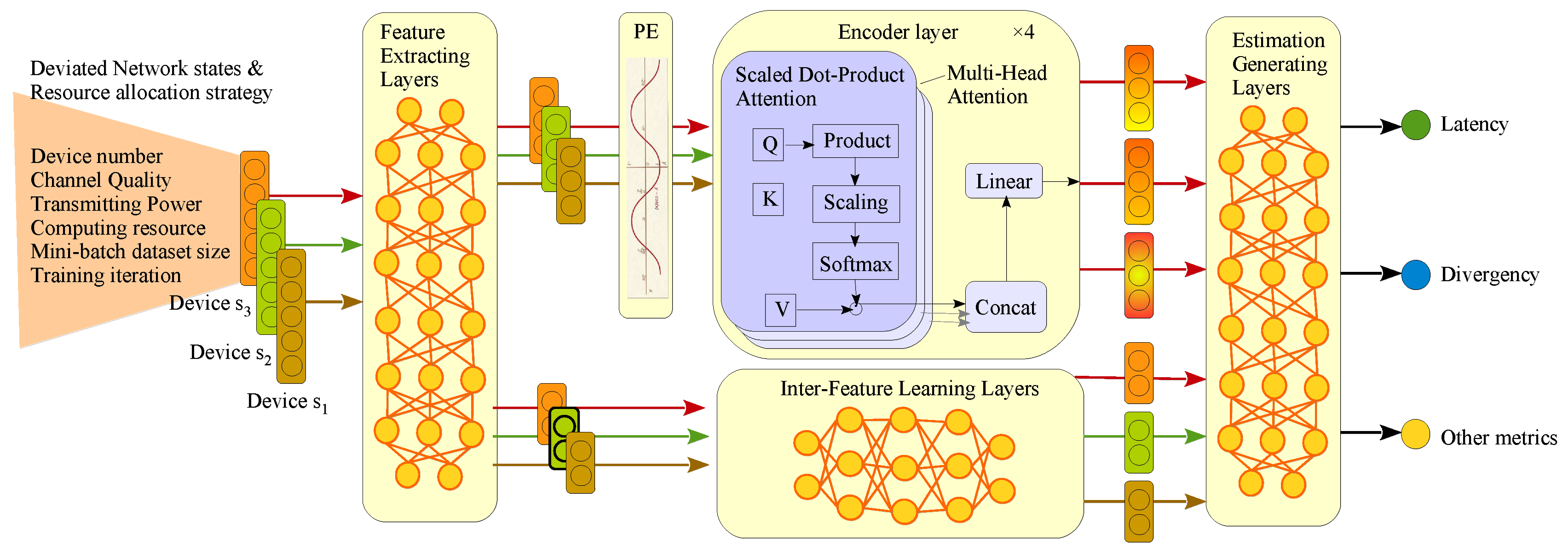
To do this, we propose a TransNeural algorithm which combines transformer with neural network to automatically learn the acquired models. First, we use neural-based feature extracting layers to automatically classify which group of features needs to model their relationships between different devices, and which group of features needs to model their inner-relationship. Then, we design encoder-based line to learn the inter-node relationships and neural-based line to learn inter-feature relationships, respectively. Finally, the outputs of two lines are aggregated using neural network to further learn the complex relationship between two lines with the estimate outputs. In addition, thanks to the added neural network in different positions, the model can learn the unknown or inaccurate parameters automatically.

Figure 2. Proposed TransNeural algorithm by combining encoder with neural network.

The proposed TransNeural algorithm can be expressed as a function

\begin{matrix} {D_{i}, ln (ε_{i})} = TransNeural ([x_{i, s_{1}}; x_{i, s_{2}}; \dots; x_{i, s_{K}}]) \\ = TransNeural ([\begin{matrix} s_{1} & H_{s_{1}}^{*} & P_{s_{1}} & f_{s_{1}}^{*} & Q_{s_{1}} & I_{s_{1}} \\ s_{2} & H_{s_{2}}^{*} & P_{s_{2}} & f_{s_{2}}^{*} & Q_{s_{2}} & I_{s_{2}} \\ ⋮ & ⋮ & ⋮ & ⋮ & ⋮ & ⋮ \\ s_{K} & H_{s_{K}}^{*} & P_{s_{K}} & f_{s_{K}}^{*} & Q_{s_{K}} & I_{s_{K}} \end{matrix}]), \end{matrix}

(23)

where all of the elements are mean normalized. The loss function is defined as

\begin{matrix} Loss = \frac{1}{B} \sum_{i} {(\frac{D_{i} - D_{real}}{D_{\max} - D_{\min}} + \frac{ln (ε_{i}) - ln (ε_{real})}{ln (ε_{\max}) - ln (ε_{\min})})}^{2}, \end{matrix}

(24)

where

B

is the size of training batch-size for the TransNeural algorithm.

2. Feature Extracting Layers

Feature extracting layers aim to automatically project different features into two groups, deciding which group of features are highly combined with inter-node relationships (such as device number) and which contribute to inter-feature learning for establishing complex relationships between network strategy and performances. Elements in different groups may overlap. We use full connected layers to construct such feature extracting layers, which can be expressed as a function by

\begin{matrix} \{Linear ([\begin{matrix} s_{1} & Q_{s_{1}} & I_{s_{1}} \\ s_{2} & Q_{s_{2}} & I_{s_{2}} \\ ⋮ & ⋮ & ⋮ \\ s_{K} & Q_{s_{K}} & I_{s_{K}} \end{matrix}]), Linear ([\begin{matrix} s_{1} & H_{s_{1}}^{*} & \dots & I_{s_{1}} \\ s_{2} & H_{s_{2}}^{*} & \dots & I_{s_{2}} \\ ⋮ & ⋮ & ⋱ & ⋮ \\ s_{K} & H_{s_{K}}^{*} & \dots & I_{s_{K}} \end{matrix}])\} \\ = FtrEtrL ([\begin{matrix} s_{1} & H_{s_{1}}^{*} & P_{s_{1}} & f_{s_{1}}^{*} & Q_{s_{1}} & I_{s_{1}} \\ s_{2} & H_{s_{2}}^{*} & P_{s_{2}} & f_{s_{2}}^{*} & Q_{s_{2}} & I_{s_{2}} \\ ⋮ & ⋮ & ⋮ & ⋮ & ⋮ & ⋮ \\ s_{K} & H_{s_{K}}^{*} & P_{s_{K}} & f_{s_{K}}^{*} & Q_{s_{K}} & I_{s_{K}} \end{matrix}]) \end{matrix}

(25)

3. Positional Encoding Layer

In SL training task, the device participate sequence greatly influence the training performance, because the initial training divergence on a new device largely depends on its data similarity with the previous training device. Therefore, we need to take the device sequence into consideration to model the relationship between strategies and SL performance. Thus, positional encoding layer is introduced before the encoder layers. Consistent with classical settings, the expression of positional encoding is based on sine and cosine functions

\begin{matrix} {PE}_{(k, 2 i)} = sin (k / 10000^{2 i / d_{model}}) \\ {PE}_{(k, 2 i + 1)} = cos (k / 10000^{2 i / d_{model}}) \end{matrix}

(26)

where k is the participating sequence of a device,

d_{model}

is the input dimension of encoder layer, and i denotes different input neural of the encoder layer.

4. Encoder Layers

The encoder layers use the classical components in encoders, including

K, Q, V

matrixes to learn the inter-node relationships by

\begin{matrix} Attention (Q, K, V) = softmax (\frac{Q K^{T}}{\sqrt{d_{model}}}) V \end{matrix}

(27)

We apply multi-head attentions to learn different kind of relationships between devices by

\begin{matrix} MultiHead (Q, K, V) = Concat ({head}_{1}, \dots, {head}_{h}) W^{O}, \\ where {head}_{i} = Attention (Q W_{i}^{Q}, K W_{i}^{K}, V W_{i}^{V}) \end{matrix}

(28)

Finally, the encoder layer can expressed as

\begin{matrix} \{μ_{s_{k}} Q_{s_{k}} I_{s_{k}}, C_{s_{k}} Q_{s_{k}} I_{s_{k}}\} = \underset{Modeling data similarities C_{s_{k}} and divergency parameter μ_{s_{k}} .}{\underset{︸}{EncoderL ([\begin{matrix} s_{1} & Q_{s_{1}} & I_{s_{1}} \\ s_{2} & Q_{s_{2}} & I_{s_{2}} \\ ⋮ & ⋮ & ⋮ \\ s_{K} & Q_{s_{K}} & I_{s_{K}} \end{matrix}])}} \end{matrix}

(29)

5. Inter-Feature Learning Layers

In the second line, we design inter-feature learning layers to non-linearly produce some key elements for estimating SL performance based on a part of features. Considering neural network are inherently good at extracting features of different levels in its layers to finally establish the complex relationships between input and output, we simply use fully connected neural network to construct the inter-feature learning layers. That is, in our scenario, the inter-feature learning layers can output wireless outage probability based on the input channel quality, and output SL latency based on the input transmitting power, computing resources, etc. At the same time, it can automatically modify the error in inaccurate computing resource and channel gain based on the device number. The function can be expressed as

\begin{matrix} \{D_{i}, [ε_{s_{1}, tr}, ε_{s_{2}, tr}, \dots, ε_{s_{K}, tr}]\} = \underset{Modeling relationships and learn accurate H_{s_{k}}, f_{s_{k}} .}{\underset{︸}{InFtrL ([\begin{matrix} s_{1} & H_{s_{1}}^{*} & P_{s_{1}} & f_{s_{1}}^{*} & Q_{s_{1}} & I_{s_{1}} \\ s_{2} & H_{s_{2}}^{*} & P_{s_{2}} & f_{s_{2}}^{*} & Q_{s_{2}} & I_{s_{2}} \\ ⋮ & ⋮ & ⋮ & ⋮ & ⋮ & ⋮ \\ s_{K} & H_{s_{K}}^{*} & P_{s_{K}} & f_{s_{K}}^{*} & Q_{s_{K}} & I_{s_{K}} \end{matrix}])}} \end{matrix}

(30)

6. Estimation Generating Layer

Two lines are finally combined in the fully connected layers, which would jointly consider the inter-node relationships and inter-feature relationships to produce the final estimated system performance, i.e., the SL training latency and accuracy in this scenario.

4. Simulation

In this section, we evaluate the proposed TransNeural algorithm in Python environment. We suppose that there are 10 devices access to an AP, where the path loss model is

(38.46 + 20 {log}_{10} (d))

[20], where d is the distance between device and AP. Each device has a unique sequence number from one to ten, which is uniquely projected to a virtual device in DTN. In addition, each device has a series of unique characteristics, which are unknown and about to be automatically learned by DTN models. Their values are randomly set as follows: distance

d_{k}^{*} \in [10, 900]

m, average reporting deviation on distance

{Δ d_{k}}^{⋎} \in [1, 10]

m, average deviation between allocated computing resource and actual provided computing resource

{Δ f_{k}}^{⋎} \in [0.1, 1]

GHz, divergence related parameter

μ_{k}^{⋎} \in [1, 10]

, each element in data similarity vector

C_{k}^{⋎} \in {\{[1, 5]\}}^{N}

. Notice that, in an SL training process, not all devices will be selected to join the training process. However, the DTN model needs to learn the characteristics of all device to better estimate the training performance for all possible resource allocation strategies. Without causing ambiguity, we use SL divergence to replace SL convergence in the simulation section, to make analysis more clearly. Other parameters are given in Table. Table 1.

Details of model in TransNeural algorithm are setting as follows. The dimension of input array is

6 \times 5

, where 6 is the maximum number of participants, and 5 is the feature dimension of one device. The structure of the feature extracting layer is

64 \times 2

, whose first layer and second layer take ReLu function and Linear function as the activation functions, respectively. The encoder block has 4 encoder layers, where each layer has 8 heads for multi-head attention, and the dimension of input vector is 64. The structure of inter-feature learning layer is

64 \times 2

, whose layers take ReLu function as the activation functions. The structure of estimation generating layer is

64 \times 2

, whose first layer and second layer take ReLu function and Linear function as the activation functions, respectively. The compared traditional algorithm estimate latency and divergency based on the equations in Section 3.1 and Section 3.2.

Figure 3 gives learning convergence of the proposed TransNeural algorithm. The figure indicates that the algorithm converges fast under various size of SL participant group. It proves that combining transformer with neural network can quickly learn the data similarities, the CSI errors, computing resource errors and other factors for devices in wireless network.

Figure 4 gives the total latency of SL training process with increasing number of SL participants. In general, the total latency of SL training increases with a growing number of SL participants, because different participants sequentially train the lower layers. Therefore, more participants will lead to a larger overall latency, which would also decrease the training divergency. In addition, the proposed TransNeural algorithm has a better latency estimation compared with traditional equation-based estimation methods. It is because that the traditional method cannot learn the deviation between the real states (such as available computing resources, channel states information, etc.) and the acquired one obtained by DTN from physical network, which is unavoidable considering the data collecting error, user misreport information, etc. As a result, the error of traditional estimations grows with the increasing number of SL participants, while the proposed TransNeural algorithm remain stable which around zero.

Figure 5 gives the total latency of SL training process with growing average distance between selected user devices and AP. In general, as the distance grows, the wireless transmission rate will first drop smoothly and then drop rapidly, which leads the transmission delay first grow smoothly and then increase rapidly. Considering the wireless transmission happens frequently in each forward and backward propagation process, the transmission delay will significantly influence the total SL training delay, which leads the total SL delay increases as the distance grows. In addition, since the DTN may not acquire accurate CSI, latency estimation based on traditional equation-based method will have a high error, especially under larger distance where CSI error becomes sensitive for latency estimation. In comparison, the proposed TransNeural algorithm has a stable error with distance growing, which stays under 100 s which omit-table because the total error is 1400-1800s.

Figure 6 gives the total latency of SL training process with a growing allocated computing resources on devices. Because user device needs to use their allocated computing resources to compute forward and backward propagation of lower layers in SL target models, the computing latency will decrease with the increasing allocated computing resources, which leads the total latency decrease. However, because of user misreport information, the real allocated computing resources may be smaller than the amount of allocated resource in network strategies, which can not be modeled in traditional equation-based latency estimation methods, leading estimation error. In comparison, the proposed TransNeural algorithm can automatically learn this misreport behaviors from historical data, thus better estimate the real latency than traditional methods.

Figure 7 gives the delay estimation error with growing CSI error and available computing resource error acquired by DTN. In general, since traditional equation-based method cannot automatically model the error in its estimating process, its estimation error will increase as the acquired error grows. In comparison, the proposed TransNeural algorithm has a stably low estimation error as the acquired error grows.

Figure 8 gives the natural logarithm of the training divergence with growing average size of mini-batch used for training on user devices. The divergence drop rapidly as the size of mini-batch grows. However, since there is state deviation in DTN state synchronization (which may lead to deviation in estimated outage probability), traditional equation-based algorithm estimates the divergence a lot lower than the actual divergency, which grows severely when mini-batch size increases, which may give the SL application company a dramatically high discrepancy when they decide to request users to provide more data for their SL training process with higher payment. In comparison, the proposed TransNeural algorithm can accurately predict the divergency under various size of mini-batch, thanks to its high learning ability.

Figure 9 gives gives the natural logarithm of training divergence with growing average distances between selected devices and AP. As distance grows, outage probability in wireless transmission process will first increase smoothly and then increase rapidly (indicating the user has approached the edge of a cell), until a distance point when it approaches one, i.e., 100% transmission failure because of bad channel quality. It will greatly influence the SL training divergence, considering the frequent wireless transmission process exists in SL training, which is also proved in the figure. In traditional equation-based algorithm, CSI error will lead to divergency estimation error, which is not obvious when devices are near its accessed AP. However, when the distance keeps increasing, the transmission quality drops rapidly, where estimation error of outage probability will become sensitive to the CSI error, until finally the outage probability approaches one, the error estimation error of outage probability will drop down to zero. The estimation error of divergency changes with the error of outage probability, which explains the triangle zone in the figure. In comparison, the proposed TransNeural algorithm can learn to automatically to cancel CSI error from historial data, thus produce accurate divergency estimation for SL training process.

Table 2 compares the estimation accuracy on SL training latency and divergence under different algorithms. As for the SL latency, the proposed TransNeural algorithm decreases the estimating deviant ratio from

14.22 %

0.78 %

, increasing accuracy by about

13.44 %

. As for the SL divergence (equal to one minus convergence), the proposed TransNeural algorithm decreases the estimating deviant ratio from

118.43 %

1.69 %

, increasing accuracy by about

116.74 %

. The table proves that the proposed algorithm can effectively improve the estimation accuracy for various types of SL metrics.

5. Conclusions

The paper closes the gap of studying the pre-validation environment for SL training tasks. It proposes a TransNeural algorithm to estimates the latency and divergency of SL training process under given resource allocation solution. In detail, the TransNeural algorithm integrates the transformer and neural network to collaboratively learn data similarities, complex relationships between SL performance (latency, divergency, etc.) and participants selections, wireless/computing resource allocation, and the reported deviation on wireless channels and available computing resources. Simulation shows the proposed TransNeural algorithm can effectively improve the estimating accuracy by

13.44 %

on latency and

116.74 %

on divergency compared with existing algorithms.

Author Contributions

Conceptualization, Guangyi Liu; methodology, Guangyi Liu, Mangcong Kang, Yanhong Zhu and Na Li; software, Mangcong Kang and Maosheng Zhu; validation, Mangcong Kang and Qingbi Zheng; formal analysis, Guangyi Liu, Mangcong Kang and Yanhong Zhu; investigation, Yanhong Zhu; resources, Guangyi Liu and Yanhong Zhu; data curation, Mangcong Kang; writing—original draft preparation, Guangyi Liu and Mangcong Kang; writing—review and editing, Yanhong Zhu and Mangcong Kang; visualization, Mangcong Kang; supervision, Guangyi Liu and Yanhong Zhu. All authors have read and agreed to the published version of the manuscript.

Funding

This work was funded by the National Key R&D Program of China (2022YFB2902100).

Institutional Review Board Statement

Not applicable.

References

Wang, Y.; Yang, C.; Lan, S.; Zhu, L.; Zhang, Y. End-Edge-Cloud Collaborative Computing for Deep Learning: A Comprehensive Survey. IEEE Communications Surveys & Tutorials 2024, 1. [Google Scholar] [CrossRef]
Wen, J.; Zhang, Z.; Lan, Y.; Cui, Z.; Cai, J.; Zhang, W. A survey on federated learning: challenges and applications. International Journal of Machine Learning and Cybernetics 2023, 14, 513–535. [Google Scholar] [CrossRef] [PubMed]
Shen, X.; Liu, Y.; Liu, H.; Hong, J.; Duan, B.; Huang, Z.; Mao, Y.; Wu, Y.; Wu, D. A Split-and-Privatize Framework for Large Language Model Fine-Tuning. arXiv 2023, arXiv:cs.CL/2312.15603. [Google Scholar]
Lin, Z.; Qu, G.; Chen, X.; Huang, K. Split Learning in 6G Edge Networks. IEEE Wireless Communications 2024, 1–7. [Google Scholar] [CrossRef]
Lin, Z.; Zhu, G.; Deng, Y.; Chen, X.; Gao, Y.; Huang, K.; Fang, Y. Efficient Parallel Split Learning over Resource-constrained Wireless Edge Networks. IEEE Transactions on Mobile Computing 2024, 1–16. [Google Scholar] [CrossRef]
Khan, L.U.; Saad, W.; Niyato, D.; Han, Z.; Hong, C.S. Digital-Twin-Enabled 6G: Vision, Architectural Trends, and Future Directions. IEEE Communications Magazine 2022, 60, 74–80. [Google Scholar] [CrossRef]
Kuruvatti, N.P.; Habibi, M.A.; Partani, S.; Han, B.; Fellan, A.; Schotten, H.D. Empowering 6G Communication Systems With Digital Twin Technology: A Comprehensive Survey. IEEE Access 2022, 10, 112158–112186. [Google Scholar] [CrossRef]
Almasan, P.; Galmés, M.F.; Paillisse, J.; Suárez-Varela, J.; Perino, D.; López, D.R.; Perales, A.A.P.; Harvey, P.; Ciavaglia, L.; Wong, L.; et al. Digital Twin Network: Opportunities and Challenges. CoRR 2022, abs/2201.01144, [2201.01144]. [Google Scholar]
Lai, J.; Chen, Z.; Zhu, J.; Ma, W.; Gan, L.; Xie, S.; Li, G. Deep learning based traffic prediction method for digital twin network. Cognitive Computation 2023, 15, 1748–1766. [Google Scholar] [CrossRef] [PubMed]
He, J.; Xiang, T.; Wang, Y.; Ruan, H.; Zhang, X. A Reinforcement Learning Handover Parameter Adaptation Method Based on LSTM-Aided Digital Twin for UDN. Sensors 2023, 23. [Google Scholar] [CrossRef] [PubMed]
Ferriol-Galmés, M.; Suárez-Varela, J.; Paillissé, J.; Shi, X.; Xiao, S.; Cheng, X.; Barlet-Ros, P.; Cabellos-Aparicio, A. Building a Digital Twin for network optimization using Graph Neural Networks. Computer Networks 2022, 217, 109329. [Google Scholar] [CrossRef]
Wang, H.; Wu, Y.; Min, G.; Miao, W. A Graph Neural Network-Based Digital Twin for Network Slicing Management. IEEE Transactions on Industrial Informatics 2022, 18, 1367–1376. [Google Scholar] [CrossRef]
Tam, D.S.H.; Liu, Y.; Xu, H.; Xie, S.; Lau, W.C. PERT-GNN: Latency Prediction for Microservice-based Cloud-Native Applications via Graph Neural Networks. Proceedings of the Proceedings of the 29th ACM SIGKDD Conference on Knowledge Discovery and Data Mining, New York, NY, USA, 2023; KDD’23, pp. 2155–2165. [CrossRef]
Vaswani, A.; Shazeer, N.; Parmar, N.; Uszkoreit, J.; Jones, L.; Gomez, A.N.; Kaiser, Ł.; Polosukhin, I. Attention is all you need. Advances in neural information processing systems 2017, 30. [Google Scholar]
LeCun, Y.; Bengio, Y.; Hinton, G. Deep learning. nature 2015, 521, 436–444. [Google Scholar] [CrossRef] [PubMed]
Popovski, P.; Trillingsgaard, K.F.; Simeone, O.; Durisi, G. 5G wireless network slicing for eMBB, URLLC, and mMTC: A communication-theoretic view. Ieee Access 2018, 6, 55765–55779. [Google Scholar] [CrossRef]
Hou, Z.; She, C.; Li, Y.; Zhuo, L.; Vucetic, B. Prediction and Communication Co-Design for Ultra-Reliable and Low-Latency Communications. IEEE Transactions on Wireless Communications 2020, 19, 1196–1209. [Google Scholar] [CrossRef]
Schiessl, S.; Gross, J.; Skoglund, M.; Caire, G. Delay Performance of the Multiuser MISO Downlink under Imperfect CSI and Finite Length Coding. IEEE Journal on Selected Areas in Communications 2019, 37, 765–779. [Google Scholar] [CrossRef]
Kang, M.; Li, X.; Ji, H.; Zhang, H. Digital twin-based framework for wireless multimodal interactions over long distance. International Journal of Communication Systems 2023, 36, e5603. [Google Scholar] [CrossRef]
TS, G. Evolved universal terrestrial radio access (e-utra). further advancements for e-utra physical layer aspects (release 9). Technical report, 3GPP TR 36.814, 2010.

Figure 3. Learning convergence of proposed TransNeural algorithm.

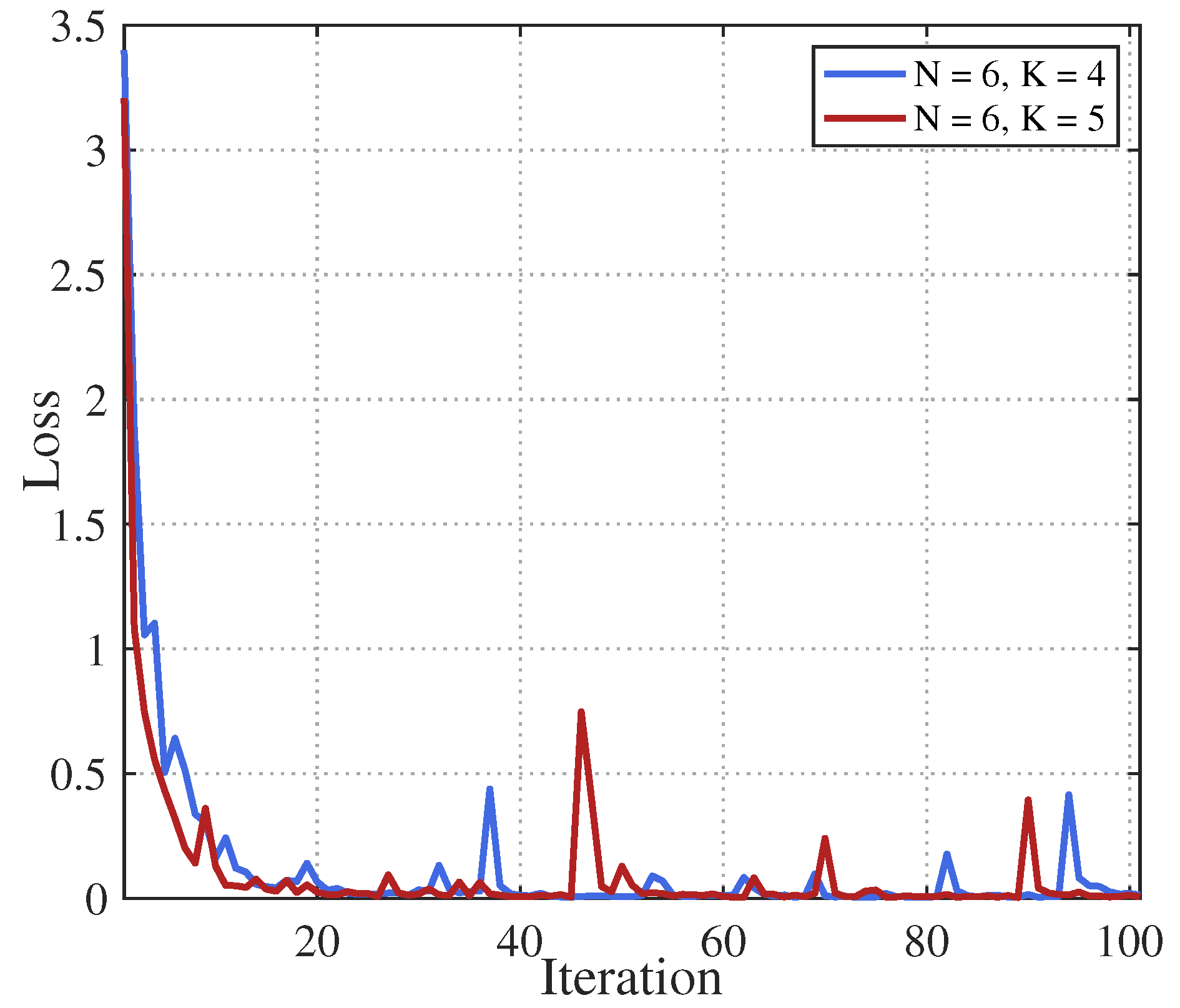
Figure 4. SL training latency vs. Number of SL participants.

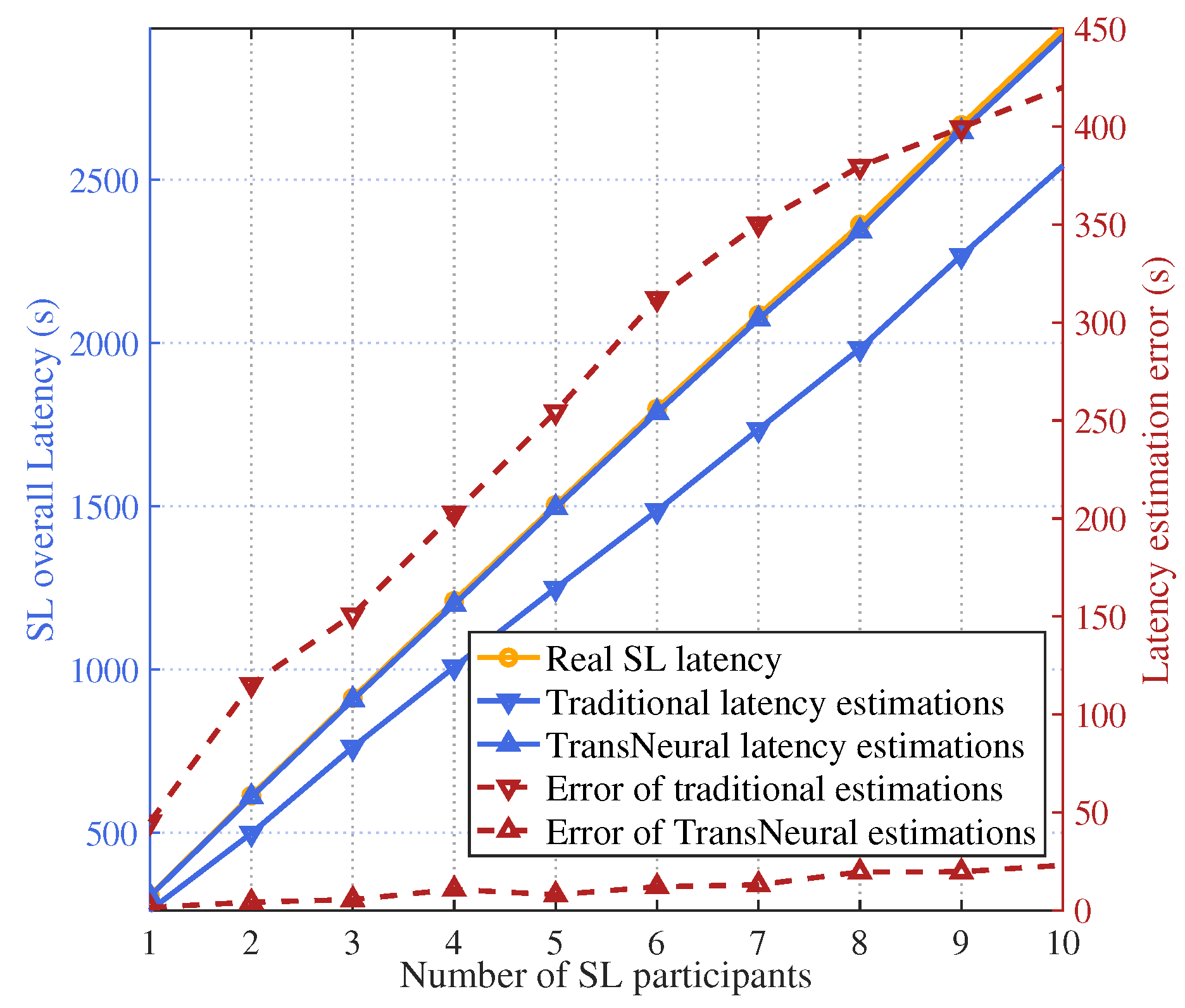
Figure 5. SL training latency vs. Distances between devices and AP.

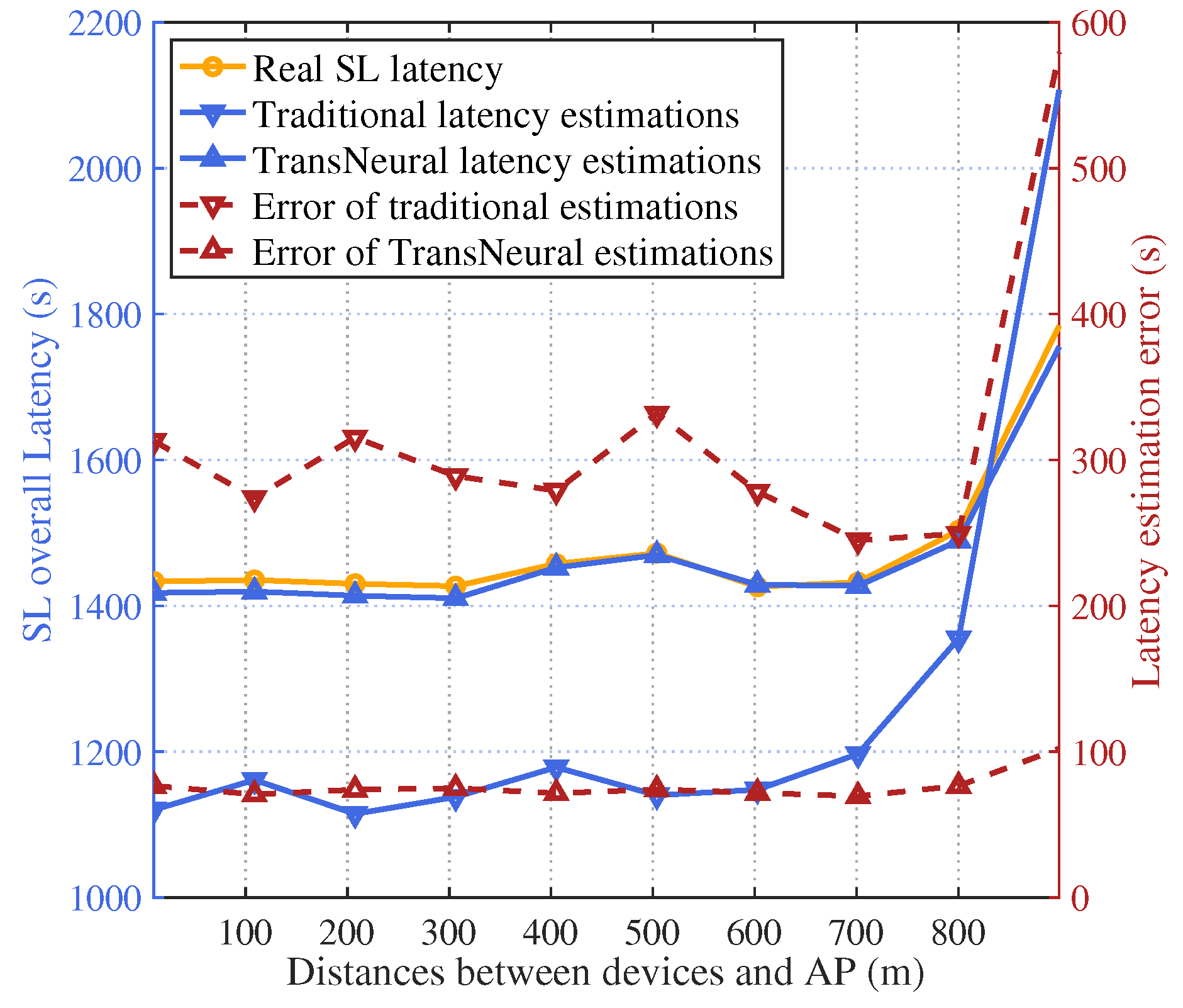
Figure 6. SL training latency vs. Computing resources on devices.

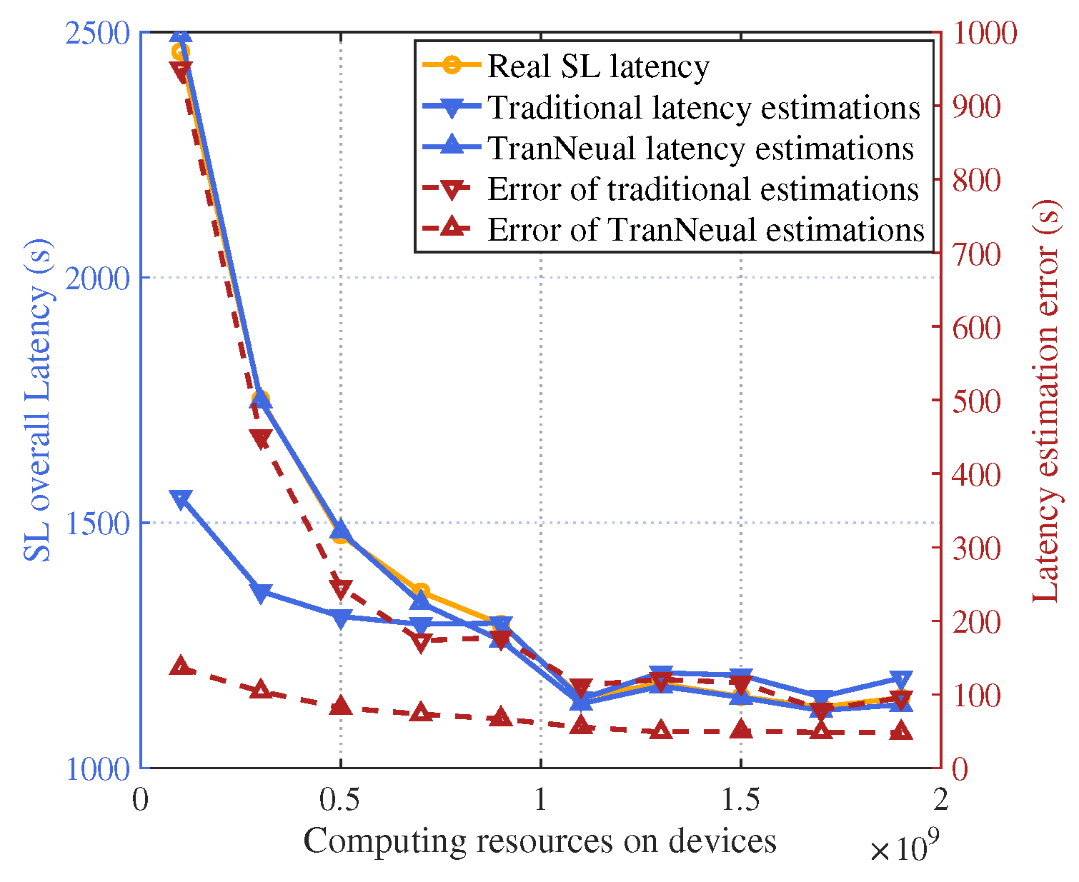
Figure 7. Latency estimation error vs. DTN data acquisition error in CSI and available computing resources.

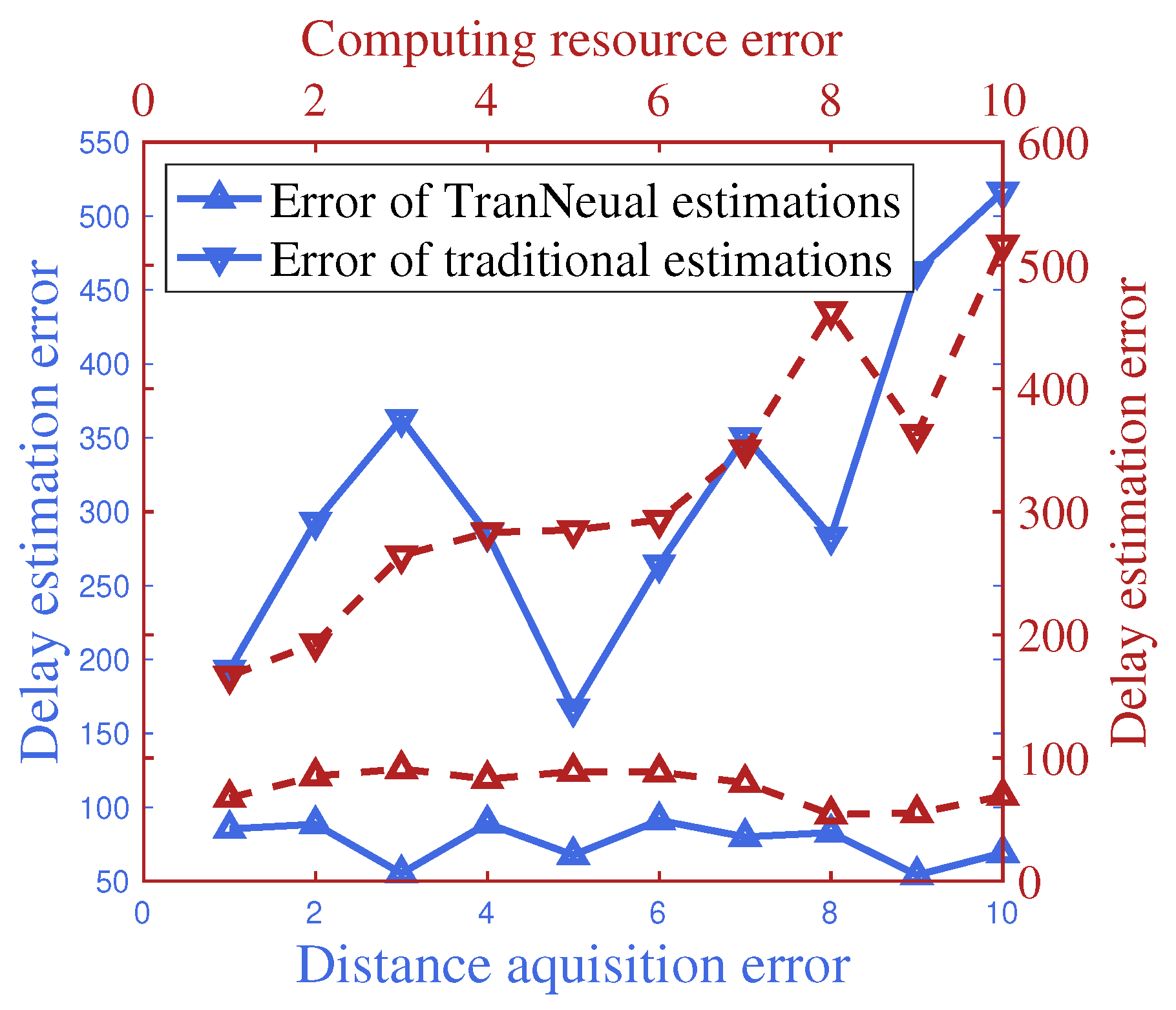
Figure 8. SL training divergence rate vs. Average size of mini-batch used for training on devices.

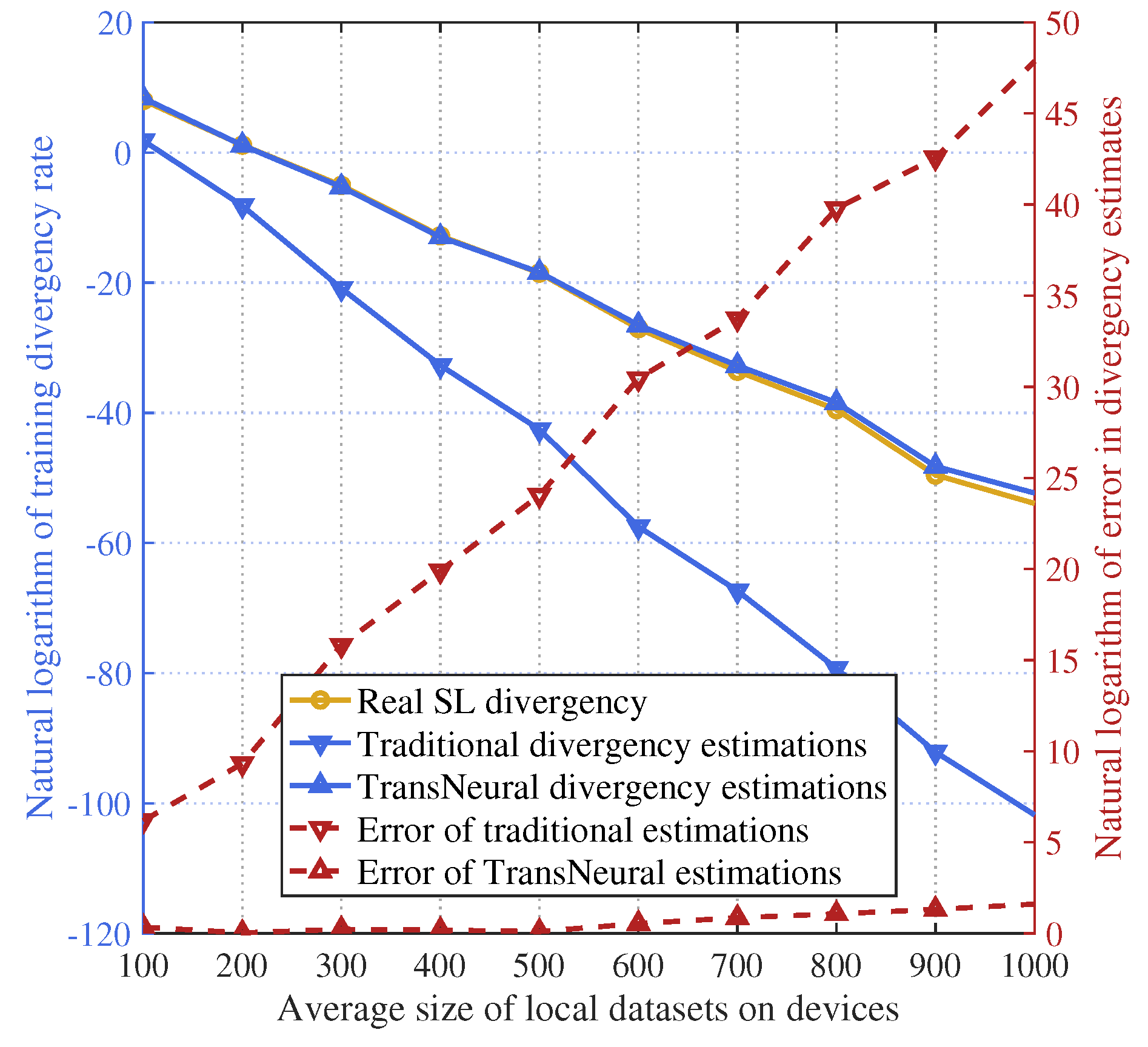
Figure 9. SL training divergence rate vs. Distances between devices and AP.

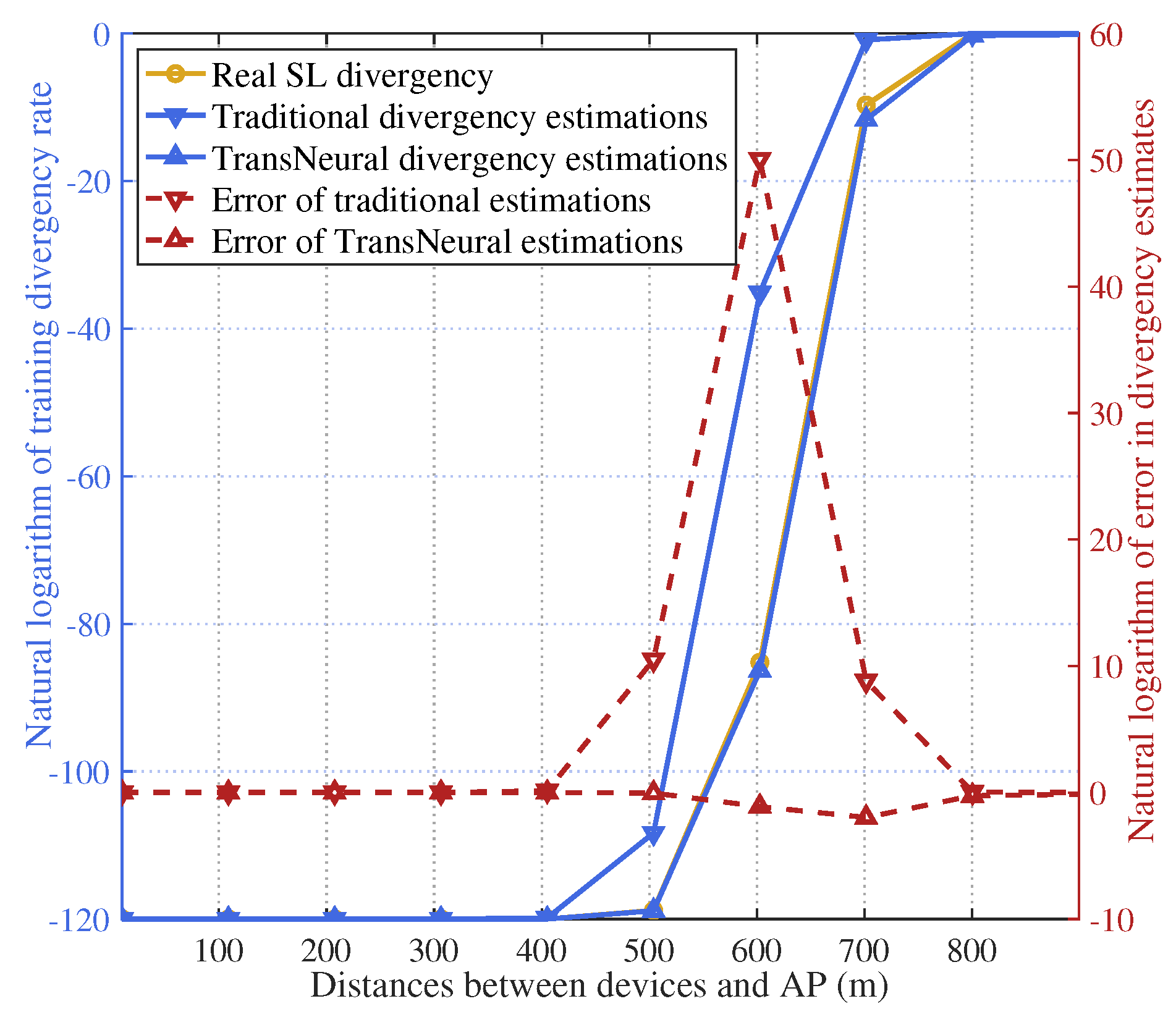
Table 1. Parameter Settings

Parameter	Value	Parameter	Value
$Q_{k}$	$[100, 1000]$	$I_{k}$	$[5, 100]$
$f_{k}$	$[0.1, 2]$ G cycles/s	$f_{B}$	100 G cycles/s
B	10 MHz	K	64
$N_{0}$	$10^{- 20.4}$	$H_{L}^{k}$	$140 \times 10^{- 6}$
$P_{k}$	$[0.01, 2]$ W	$P_{B}$	88 W
$b_{mid, fw}$	1 Mbits	$b_{mid, bk}$	1 Mbits
$c_{up, fw}$	100 M cycles	$c_{up, bk}$	100 M cycles
$c_{lwer}^{forward}$	1 M cycles	$c_{lw, bk}$	1 M cycles
$b_{lw}$	1 Gbits

Table 2. Comparison of deviant ratio for estimated latency and divergence in SL training process

	Latency estimation (s)	Deviant ratio
Actual SL latency	$296.26$	/
TransNeural algorithm	$293.94$	$0.78 %$
Equation-based algorithm	$254.12$	$14.22 %$
	Natural logarithm of convergence estimation	Deviant ratio
Actual SL divergence	$- 22.87$	/
TransNeural algorithm	$- 22.48$	$1.69 %$
Equation-based algorithm	$- 49.96$	$118.43 %$

Disclaimer/Publisher’s Note: The statements, opinions and data contained in all publications are solely those of the individual author(s) and contributor(s) and not of MDPI and/or the editor(s). MDPI and/or the editor(s) disclaim responsibility for any injury to people or property resulting from any ideas, methods, instructions or products referred to in the content.

© 2024 by the authors. Licensee MDPI, Basel, Switzerland. This article is an open access article distributed under the terms and conditions of the Creative Commons Attribution (CC BY) license (http://creativecommons.org/licenses/by/4.0/).

Copyright: This open access article is published under a Creative Commons CC BY 4.0 license, which permit the free download, distribution, and reuse, provided that the author and preprint are cited in any reuse.

Downloads

Views

Comments

Subscription

Notify me about updates to this article or when a peer-reviewed version is published.

MDPI Initiatives

Important Links

Choose an area of interest and we will send you notifications of new preprints at your preferred frequency.

Disclaimer

TransNeural: An Enhanced-Transformer based Performance Pre-Validation Model for Split Learning Tasks

Abstract

Keywords:

Subject:

1. Introduction

2. System Description

2.1. System Model

2.2. Communication Model

2.3. Split Learning Process

2.4. Digital Twin Network

3. Transformer-Based Pre-Validation Model for DTN

3.1. Problem Analysis for SL Convergence Estimation

3.2. Problem Analysis for SL Latency Estimation

3.3. Proposed Transformer-Based Pre-Validation Model

4. Simulation

5. Conclusions

Author Contributions

Funding

Institutional Review Board Statement

References

MDPI Initiatives

Important Links

Subscribe