Submitted:
21 June 2024
Posted:
24 June 2024
You are already at the latest version
Abstract
This document introduces methods and algorithms to characterize a series of values as patterns of repeating symbols or sequences selected with the criterion to maximize the information retrieved. The method converts a series of real-number values into texts. Then, it interprets the text from a point of view specified by several parameters. Located patterns are linked nested, with shorter sequences within longer ones. Texts are then synthesized and organized in a tree-like structure, substantially reducing entropy. The characterization of processes serves as the basis for constructing models to estimate likely projected values. Alternative ways to assess the multiscale complexity of unidimensional processes are applications of the results obtained here.
Keywords:
patterns
; nested patterns
; information
; entropy
; ordered structure
; redundancy
1. Introduction
Patterns are the essence of information. Sometimes established, sometimes waiting to be discovered, patterns comprise a world of interpretations and assigned meanings. Patterns are how nature organizes itself. However, patterns are also the means to interpret and advance our understanding of nature. Our knowledge is based on patterns. Number systems assign a sense of quantity to the patterns formed by elementary symbols. Languages consist of rules governing the formation of patterns to create messages, descriptions, and models. Despite the mechanism of associating patterns to produce a communication channel, an abstract perspective is often the approach to study patterns. The semantical meaning, if there is any, is not as important as the quantity of information a pattern can bring with it and how this information quantity varies as the same data set obeys different observation criteria: different interpretations. In 2021, Duin [1] presented an extended treatment of the types of patterns and their relevance in human knowledge development.
The summation of several known periodic time functions or signals typically models periodic time functions or signals. Among the functions used when this approach applies are Sines, Cosines, and Wavelets. Fourier and Wavelet analysis led to the algorithmic cornerstone of the periodic and stationary signal processing tool: the Fast Fourier Transform (FFT). Nevertheless, nonstationary phenomena escape from the Fourier Transform’s capacity to represent them in the domain of frequency. In the comprehensive introduction of their paper, Huang et al. [2] mention the disadvantages of other strategies to decompose a nonstationary series of values. In the same paper, they introduced the Empirical Mode Decomposition (EMD), an alternative method to study nonstationary systems. According to Mahenswasri and Kumar [3], the EMD enjoys popularity in addressing engineering, mathematics, and science problems. In the search for a faster method, Neill [4] published a method based on a data sample indicating that potentially relevant patterns are detected.
Besides the non-periodicity, another aspect that adds difficulty to the series synthesizing process is nested pattern detection. Despite its promises, nested pattern detection poses formidable challenges. The inherent complexity of nested structures demands innovative approaches and specifically developed computerized tools that can disentangle overlapping patterns and discern hierarchical relationships.
Detection methods inspect data sets to detect patterns. Traditional methods locate repeated symbolic sequences within a long text. Typically, once the localities of a repeated sequence are determined, the space occupied by these sequences is isolated, and the search for more repeated sequences continues over the remaining text. Thus, the procedure does not further search for repeated sequences within the repeated sequences found; it does not further search for nested repeated sequences. We refer to this type of procedure as the zero-depth text interpretation. In contrast, if the inspection continues looking for repeated sequences within the already found longer sequences, we call the procedure a nested pattern detection method.
The paper explores nested pattern detection, leaning on the power of a software platform tool named MoNet [5]. MoNet comprehends tailored coding pseudo-languages designed to operate with complex data structures as multidimensional orthogonal arrays and data trees. MoNet handles these structures as elementary objects allocated in a single memory address; at the same time, they can also be partitioned according to desired segmenting criteria. The document offers methods, including converting numerical series into alphabetical texts, characterizing unidimensional processes by detecting nested patterns, and a probability-tree projection model.
2. Interpretation Models for Unidimensional Descriptions. Sequence Repetition Model
Consider text formed by a series of elementary characters ; each referred to according to their position in . Then, the text can be expressed as the following concatenation of characters:
We define the interpretation process, or simply the interpretation, as the criteria to form groups of characters that reduce 's complexity. The interpretations inspect text for sequences of characters that appear or more times. The term 'symbol' refers to these characters' sequences. Nevertheless, sometimes, we use the term 'sequence' to recall the symbols, which are, within the scope of this document, strings of neighbor characters. After submitting a text to any process capable of retrieving the repeated char sequences or symbols, we may represent the resulting set of symbols, with their corresponding frequencies of occurrence , as:
Notice that the series of symbols and frequencies start at index . That means the number of repeated symbols is . Equivalently, the symbolic diversity of is .
When interpreting text at its maximum scale, sub-contexts are not considered, thus, there must not be overlapping positions occupied by any two symbols. Consequently, symbols must not share any char position. Interpretations of text may differ when diverse criteria are used to select, within the text, the sets of contiguous characters to form a set of symbols . Based on the observer’s choice—or the choice implied by the observer’s criteria—, a symbol starting at the text-position , and made of characters is
Additionally, all chars contained in are not necessarily part of a symbol in the set . The chars not included in any are noise concerning the interpretation. This consideration is consistent with the typical existence of not synthetized fragments in any system’s description. However, the standard objective of any description is to minimize the noise fraction.
For long texts and time series, the symbol diversity may be significant. In these cases, reducing the complexity of the system’s representation is convenient to make it feasible and controllable for a quantitative analysis. To cope with this, we propose working with the set of symbols grouped by their length. Therefore, we define as the set of all repeated sequences sharing the length . Correspondingly, let be the number of appearances of each symbol category . Thus, the tendency of a process to repeat sequences of values according to their lengths can be characterized by the spectrogram , which we defined as
where and are the length and the frequency of the longest repeating sequence within text .
The frequencies are linearly related to the fraction of text occupied by symbols of each length category. Then, by convenience, we alternatively express the characteristic spectrogram in terms of the probability of encountering a -long sequence within text .
We refer to the spectrograms and as the frequency-based and probability-based Interpretations. We use the term Representation to refer to the selections of char-sequences to form sets of symbols and obtaing after some Interpretations
2.1. Probability Model of the One-Scan Repeated Sequence Length (OSRSL)
We aim to build a probability model of the repetitions of sequences of similar values in a series. In this context, similar values refer to data elements sharing the same category in a discrete quantitative scale. When the original data is a series of scalar numbers, a meticulous discretization step converts the values into a text formed with an alphabet of as many letters as the resolution of the discretizing process requests. This precise process identifies repeating sequences within the text , and as a result, and are the lengths and the frequency of the most extended repeating sequence. From our perspective, such a probability model would be an interesting tool for extracting information on the process values, creating a “fingerprint” of the process behavior, and facilitating a deeper understanding of the process.
We expect to deal with complex processes that usually are oscillatory but non-periodic series of values. The Discrete Fourier Transform (DFT) algorithm is the classical tool to study oscillatory processes. However, the DFT is not well suited for low frequency and non-periodic processes [6], and its complexity [7] may represent a barrier with series in the order of thousands of values. Our approach to achieving this objective is to build the probability distribution of char-sequences—or symbols, as we have defined them—that repeatedly appear in a text. The aleatory variable is not the sequence but the repeated sequences’ length measured in the number of chars. Inspecting the text to locate the most extended repeat sequence and then using the results to compute the probability associated with each sequence length is time-consuming. That procedure would require running times the Repeated sEquence eXtractor (REX) algorithm—explained later in this paper—to determine all elements on the right side of Definition (5). Thus, we first focus on answering these questions: Having a text , which length is , and what is the most extended sequence that appears or more times in a text? How long is the sequence? Once this step is accomplished, the found repeated sequences are isolated from , leaving the text , whose shorter length , remains to be analyzed in further steps with an overall convenient algorithmic complexity reduction.
We start with a -character long text , formed by different chars distributed along the text. By locating the most extended no-overlapping sequence appearing times in text , we empirically compute the probability of containing an -long sequence that repeats times. At this point, we introduce the syntax to refer to the likelihood of a -long sequence appearing exactly times in the text . After scanning the text and identifying the -times repeating sequences, we write:
Following the computation of the probability , the search for repeated sequences continues with the remaining text of length . Identifying the length of the most extended repeated sequences at each search step leads to determining the probability referred to the length of the remaining text corresponding to the step . Thus,
After applying the algorithm REX and identifying the most extended repeated sequences for , , , and successively using Equation (7), intermediate probability results are obtained. The values of probabilities exhibit an attractive distribution that is convenient to discuss here. Note the remaining text fraction reduces every time REX isolates the found sequences until no more repeated sequences are found. The final remaining text not represented by any repeated sequence is an expression of noise contained in the original text .
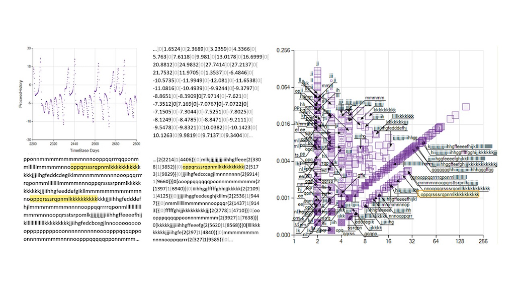
Figure 1 (Left) shows the origin of the ramp-shaped probabilities . Figure 1 (Right) is an actual graph showing the interpretation of results .
The probability distribution of the One-Scan Repeated Sequence Length (OSRSL) retrieves a set of character sequences that appear in such frequencies that they minimize the symbol frequency-based text description; therefore, a relatively low entropy description is reasonable to expect. Since this condition implies interpreting the text to maximize extracted information, we regard this resulting set of symbols as a scale of observation. It is worth mentioning that the OSRSL determines this observation scale by locating sequences from the longest to shortest ones, contrasting the procedure followed to determine the so-called Fundamental Scale [8], which searches for repetitive sequences starting from the shortest to the longest one.
The OSRSL characterizes the process by modeling it through the first-scan interpretations and defined in (4) and (5). However, these interpretations are only a top-scale characterization of . Successively repeating the process on each sequence is performed to obtain a nested sequence-length characterization of the text, as is presented in the section below. On the other hand, by comparing with the first OSRSL scan offers a measure of the noise integrating interpretations and .
2.2. Nested Repeated Sequence Length Decomposition (NRSLD)
Looking for symbols repeated within another symbol, as in a nested fashion, would alter the scope of the observer’s view. Considering ‘nested contexts’ is needed to assess the complexity of a system integrating all possible scales of observation. In this section, we explain a procedure to obtain these sets of sequences, which we name the Nested Repeated Sequence Length Decomposition (NRSLD). By studying the NRSLD associated with a process text, we expect to characterize the process. However, decomposing a long text in the repeated sequences on their length is a highly long computational operation. Without a pre-established sequence repetition pattern, the text must be scanned an enormous number of times while accounting for the number of each character-sequence that appears repeatedly in the text. Consequently, we look for a scanning criterion to constrain the scanning branches through the text and lead the procedure to a feasible condition.
In a former section, we presented the OSRSL, a procedure conceived to retrieve the most extended character sequence that appears at least times. After blocking the sequences found, the remaining text is subject to inspection to retrieve the following most extended sequence that appears times. The search for repeated sequences continues until the remnant text does not contain repeated sequences of two or more characters. The OSRSL is a valid characterization; however, since every found sequence is isolated from the search space, the OSRSL does not account for the number of times shorter sequences appear contained in a longer sequence. Thus, the OSRSL does not directly capture the potential characteristic behavior. A way to accomplish our goal of building a probability distribution expressing the fractions occupied by repeated sequences in the full range of the text is to complement the distribution represented by OSRSL with appearances of the short sequences that may be within the longer—previously blocked—sequences. This strategy, fully explained in the section below, leads to the Nested Repeated Sequence Length Decomposition (NRSLD). The NRSLD not only expresses the tendency of the text-represented process to repeat state sequences but also offers a characterization of the system structure by showing how deep a sequence is nested within more extensive char sequences.
The syntax refers to the probability of an -long sequence appearing exactly times in the text . The sub-index denotes the specific sequence. To compute the likelihood , we account for the sequences nested into longer repeated sequences that function as text containers. The account starts from the repeated sequences encountered by the OSRSL: the probabilities . The found sequences are isolated from , and the remnant text is subject to a similar search for repeated sequences; this procedure segment repeats until the remnant text is not long enough to contain repetitive sequences.
At the end of this initial stage, we see text at its maximum scale. We conduct the text observation scope using its depth . The observation depth determines the text description—and, therefore, the process represents—through the set of the repeated sequences found in . Consistent with the scale concept proposed by Febres [9], the text broadest observation scale description is the set of repeating sequences found at the nesting depth . After completing this stage, the procedure follows similar steps, accounting for the sequences that appear nested at one additional level within the more extensive sequences. We call the structure resulting from this procedure The Nested Decomposition. The repeated sequences detected at each inspection depth constitute the set of sequences corresponding to more detailed observation scales. The text fraction that a repeated sequence occupies grows with , the sequence’s length, and , the number of times it appears in the text. Therefore, we determine the NRSLD elements—the values—by adding the probability OSRLS of appearances of shorter sequences nested in the longer sequence; the value tends to increase proportionally to the product . Thus, we write . However, since and grow in opposite directions, we do not expect to increase or diminish indefinitely. Nevertheless, since shorter sequences may appear nested at several depths in longer sequences, values are expected to differ by several orders of magnitude as their length varies, thus making our selection to represent the NRSLD as a log-log diagram.
The NRSLD graphically describes the tendency of a process to repeat strings of states—namely sequences—. Graphically expressing how these strings nest into longer ones requires adding attributes, like colors or transparencies, to the bubbles representing sequences, a promising and fascinating graphic objective we may further develop in a later paper. In this document, we explore two graphic representations of the NRSLD:
- MSIR: Multiscale Integral representation. It comprises the sets of symbols sharing their length and disregarding the nesting depth they appear at.
- NPR: Nested Pattern representation. It regards the symbols’ nesting depth within the tree structure.
Figure 2 illustrates two representations of repeated sequences' probability decomposition according to length. Figure 2 (Left) shows bands where the results of the NRSLD are expected to lie for a 10000-char-long text. Figure 2 (Center) shows the MS representation of an actual NRSLD performed over a 10000-char-long text. Each triangular bubble represents the set of all repeated sequences of the same length; there may be several different sequences in a sequence, but all sequences in a set share the same length, represented in the horizontal axis. The vertical axis shows the fraction of space occupied by the same length sequence set. Note that these sequences belong to a same-length set independent of how nested each sequence appears within longer sequences, which explains why the summation of space filled by sequences adds up to more than one. In Figure 2 (Center), therefore, the vertical dimension represents the probability of encountering a sequence of the length signaled in the horizontal axis within the text; the MSIR. Figure 2 (Right) shows the unfolding of the NRSLD and the same-length sequences into sets sharing the same nesting depth; the NPR. Large bubbles correspond to the shallowest nesting depth, while progressively smaller bubbles indicate smaller and deeper nesting symbols appearing in the text as components of more extensive sequences.
3. Pattern Detection
A pattern is one of those concepts that is difficult to describe. It is not trivial to depict a pattern without using the word pattern or an equivalent symbolic representation. The Oxford Dictionary defines a pattern as “the regular way something happens or is done.” The qualification of “regular” overcomes the difficulty of defining a pattern. However, there remains highly subjective content in the word ‘regular,’ compromising the actual meaning and usefulness of the definition.
In this study, we call a pattern the description of the inscribed at least times in text . When searching for char-sequences repeated or more times, the procedure scans the text priorizing long sequences over short ones. Then, we need a procedure to find repeated sequences that appear the required number of times, at any search cycle: the Repeated sEquence eXtractor (REX) algorithm.
3.1. The Repeated-Sequence Detection Strategy
Repeated sequence detection involves encountering the symbol sequence that maximizes a specific measure or function within a large symbol string. Thus, we infer that the longest repeated sequence best represents the larger context where the repeated sequence exists. Repeated sequence detection should be distinct from pattern search algorithms, which determine the position where a specific sequence exists within a large symbol string. Our strategy to detect repeated sequences is based on the C-Sharp method IndexOf(TheInspectedPhrase, TheSoughtSequence) which returns the first position, from left to right, where the TheSoughtSequence appears within the larger text TheInspectedPhrase. The method IndexOf(), as any equivalent procedure in another computing language, belongs to the so-called Pattern Search algorithms. The search procedure we propose intensively uses the method IndexOf(), however, these are elaborated routines that realize this complex pattern detection. Consider the char-string X forms the -long sequence of elementary characters :
The most extended sequence of chars that appears at least times within text reveals the most significant pattern emerging in this context. The procedure consists of two code loops named the Outer and the Inner loops, which control the position and the size of a sliding window, respectively. The search starts from the left extreme of the text , forming an evaluation window that slides to the right as the Outer loop progresses (see Figure 3). Every time the Outer loop scans , looking for sequence repetitions, the window’s length sets to the maximum sequence size that could repeat times: . For each Outer loop index, the Inner loop tests decrease the size of the sequences evaluated until locating an -times-repeated sequence or until reaching the minimum size of a compound sequence, which is 2. When an Outer loop ends the procedure identifies an -times-repeated sequence, the spaces occupied by these sequences are isolated from the text, and the Outer loop begins again while excluding the isolated characters from the remaining text that is still to be processed. It is worth highlighting that these two loops run and inspect all possible combinations of the sequence’s length and starting position for repetitions.
Every time the sliding window sets in a new position, the function IndexOf() detects the next position the same symbol sequence appears to the right. IndexOf() is successively applied while accounting for the times the symbol exists. During the processing scan of the Outer and Inner loops, only the symbol subsequence with the maximum value of the SymbolRelevance() is retained in memory as representative of the most significant pattern detected so far. After completing the loops, the symbols excluded from the repeated sub-symbol strings are tagged as unallocated. The unallocated strings are subject to the same process of allocating shorter repeated sequences within the forming coexisting patterns.
The SymbolRelevance() function considers the option the user selects. Symbols' relevance is assessed by setting criteria of sequence length, sequence frequency, or a combination of both may be selected. In this study, we selected the criterion of priority given to the sequence length. The SymbolRelevance() function also has a parameter to activate symmetric sequences as valid repetitions. Thus, if the Symmetry Parameter is activated, then the text "hgfedcba" is accounted as a repetition of the sequence "abcdefgh," and vice versa.
3.2. The Symbol-Length Growth Mechanism
An aspect of the method worth mentioning is the process of the first found -repeating sequence to determine the most extended sequence that repeats within the text at least times. Finding an -repeating sequence within a text is time-consuming, especially when the search starts with a disoriented idea about the sequence that is likely to appear in the text at least times. However, suppose the sought sequence is short in terms of characters. In that case, the probability of finding a repeated sequence increases dramatically, and thus, the time required for the search reduces by orders of magnitude. This idea effectively reduces the task time by starting the repeated sequence search with a short char-sequence symbol. Once the procedure identifies a shorter sequence that repeats at least times, forming longer sequences by adding neighbor characters and searching for repetitions of them is faster. Figure A11 shows a pseudo-code of the procedure RepeatedSeqGrowth().
3.3. Criteria for Interpretation
We showed a procedure to determine the repeated symbol contained in a series of chars. This text comes from an established series of characters in a particular alphabet. As examples of such a character series, we mention the sequences of any alphabetic natural language or a sequence of a DNA chain segment. In these cases, the meaning of any character exists independently of interpretations. Nonetheless, detecting a repeated sequence may depend on the criteria used to prioritize the repetitive symbols identified to represent the intended interpretation of the text.
We can think of many criteria that can be applied using the function SymbolRelevance(), shown in Figure 4. Many criteria could be considered: symbol length, symbol frequency, diversity of chars in symbols, and symbol’s char-entropy are examples. Figure 4 presents several stages of detecting repetitive sub-sequences while applying the symbol frequency and symbol length criteria to a short string text form with a five-char alphabet for illustrative purposes. The more suitable interpretation depends on the parameter that best represents the objective behind the observation: long repetitive symbols or widespread symbols.
Applying the algorithm allows us to consider our natural observation process to build plausible criteria for detecting patterns and to form an interpretation of the text. We focus on the most significant objects that appear more than once within our sight scope (interpretation 1), or we pay attention to the most repeating objects (interpretation 2). After fixing the perception of the most prominent sub-sequence of characters, we release our attention on them and consider the remaining scope to repeat the same process in the next step.
3.4. The Repeated sEquence eXtractor (REX) Algorithm and the OSRSL
The pattern detection strategy, the symbol-length growth mechanism, and the interpretation criteria explained above integrate the Repeated sEquence eXtractor (REX) algorithm. A Pseudocode is incuded in the Figure A11.
REX sets , the maximum length of a sequence that may appear times in the L-long text. Afterward, REX forms a sliding window containing a sequence of length . For each sequence length , REX scans the text and registers the result whenever the sequence appears or more times. This scan is performed in a code loop testing sequences and diminishing by one the sequence’s length at each loop’s cycle. Thus, the complexity of REX is proportional to . In some situations, as a DNA string, is large, therefore, fractioning the original text might be an option. Estimating the length of the longest -times repeating sequence also helps to maintain conveniently low. On the other hand, cannot be higher than , therefore, lower required repetitions values produce larger bounds for and consequently longer—sometimes prohibitive—times to reach results.
The algorithm REX retrieves a pattern description of the submitted text. A tree-like structure expresses the result containing each symbol detected, the frequency, and the positions where each symbol instance appears within the text. Figure 4 shows two interpretations of an example text submitted to the nested decomposition. These representations include the syntactical form and the tree structures corresponding to both interpretations. By extracting the properties of the resulting structure, we can characterize each of these trees representing different interpretations. A set of parameters (: the number of instances required to be considered a repeated symbol, : alphabet size/resolution, symmetry, and other criteria) define an interpretation. We see the place where these parameters’ values may exist as the space where studying the effectiveness of the process is possible. Therefore, selecting the parameters that best fit an objective or purpose gives us a valuable tool to analyze and describe complex unidimensional texts representing systems’ behavior.
A result of each interpretation is the probability function based on the length of the repeating symbols. In other words, the result is the data used to build a probability model, such as the one expressed in Equation (7). By extracting and arranging the symbol frequencies and considering the length of symbols, we can account for the space of the text covered by repeated symbols upon their length. By scaling these counts with the number of symbol instances detected, we obtain a probability model corresponding to an interpretation. The model, in turn, serves to quantify the text’s tendency to repeat sequences of specific lengths as is seen from a maximum scale point of view.
The space structures depicting the interpretations directly obtained from REX contain information referring to each repeated sequence found and each sequence instance position within the text. This structure is detailed up to the point that it may provide more information than we can handle to reach an adequate synthesized text description from our ‘macroscopic’ point of view. To reduce the description’s complexity, we group all sequences into sets of symbols sharing their sequences’ length. We computationally add up the probabilities corresponding to the symbols with the same length to obtain probabilities . After this procedure, we get the OSRSL as the one shown in Figure 1 (Right). The model OSRSL describes text as it looks from the outside, detecting the structure that can be formed with the most extended non-overlapping elements forming the text, thus disregarding internal links among the elements that could appear from more profound points of view.
3.5. The NEsted Sequence TExt Decomposition (NESTED) Algorithm and the NRSLD
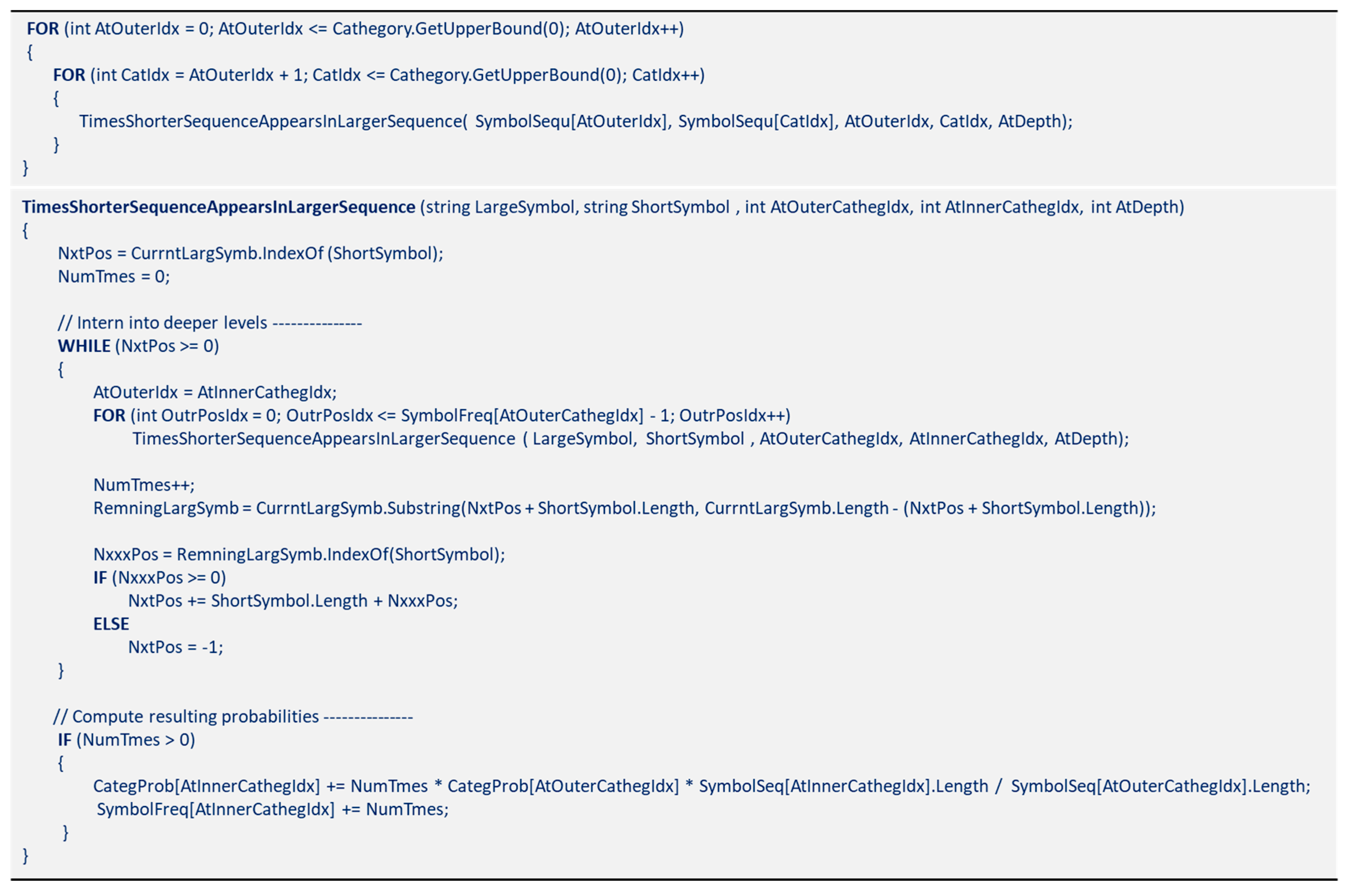
The NRSLD is algorithmically obtained from the results of the OSRSL The NEsted Sequence TExt Decomposition (NESTED) algorithm starts with the equally long symbol sets and recursively scans them, looking for nested appearances of shorter symbols located in longer ones. Figure A13 includes a Pseudocode of NESTED.
3.6. Nested Pattern Complexity (NPC)
Arguably, the number of sequences located at each nesting depth is intimately related to the structural complexity of the process the text is representing. We need to find a term to name this property. A close term is ‘Nestedness’, which was created by biologists to categorize structures in ecological systems. However, it refers to the distribution of species concentrations in an ecosystem [10]. BarYam [11] proposed complexity profiles to assess the complexity as a function of the scale observation level. BarYam’s complexity profile depicts the impact of the observation scale, retrieving the complexity associated with the system description realized at a specific observation scale. After applying the NESTED algorithm, the NRSLD describes the Text as a tree structure. The NRSLD is a tree-shaped structure. The text description is modeled as large components containing elements until the smallest components—the leaves located at the deepest nested level—are reached. This tree-shaped structure is, therefore, generally fractionally dimensioned between one and two. We assess the complexity of this tree structure as the summation of the information needed to describe each tree’s node. We refer to the complexity of this fractal-like structure as the Nested Pattern Complexity (NPC).
Figure 5 (Right) shows the terms used in this computation. A node located at tree depth , that is the ’st son-node of its parent node, represents the symbol which appears times at depth in the text . The diversity of symbols describing node is , equal to the number of symbols—repeated sequences—contained in .
Using Shannon’s entropy to assess the information needed to describe node , we compute ’s complexity. The logarithm’s base in Equation (8) equals the symbolic diversity to normalize the result to a symbol diversity different from 2, the standard case for binary trees. Equation (8), then, produces a Real number between zero and one (0-1), where zero corresponds to systems consisting of only one type of element, and one (1) corresponds to a system described with groups of types arranged without detectable patterns, and therefore, showing the maximum disorder. As Equation (9) suggests, adding this information measure from node to the last node obtains the information needed to describe the complete nested pattern structure representing the system: the NPC of the full-text .
Describing system ’s as signaled by Equation (9) relies on the NRSLD, which detects and organizes the primary symbols in and structures them in a tree-like shape. Since the NRSLD extracts patterns—or information—from , we hypothetically expect a complexity reduction reflexed in the NPC. The NPC value depends on the shape of the tree-like structure derived from the interpretation applied by the NRSLD. Consequently, this complexity reduction, hypothetical so far, is due to the order the algorithm NESTED imposes in how it looks and interprets text . Given the many shapes the tree structure may adopt, it is reasonable to expect a relevant complexity reduction from at least some of the feasible interpretations the algorithm NESTED provides.
Aiming to understand the complexity reduction associated with the NPR, we compare the NPC with the complexity of the set of symbols NESTED identified but disregarding the information provided by each symbol's nesting depth. We call this complexity figure the Multiscale Integral Complexity (MSIC). The MSCI figure is equivalent to the complexity of a unidimensional string of symbols, all existing at zero depth under the root node. Thus, we can use Equation (8) to figure MSIC. A later section compares the results of NPC and the MSIC.
4. Discretizing Numerical Series of Values
The proposed pattern detection method is a compound procedure that combines, among other aspects, setting scale limits, resolution adjustments, scale linearity changes, symbol sequences alignment, recursion, and optimization. It resembles a variational calculus applied to a discrete functional field. The approach consists of detecting repeating sequences in a long string of symbols and configuring a space of possible patterns that characterize the subject string. These prospective patterns are compared with each other to select the combination that best represents the subject string based on a defined interpretation objective.
Usually, the subject of study is a series of numerical values. One initial step in the pattern detection process is to build an -long sequence of elementary symbols—or chars—that represents the original numerical value series in that this symbolic string resembles, at some scale, the “rhythm of variations” of the numerical series. We refer to this step as discretizing. The quality of the resemblance between the symbolic string and the series of values achieved after discretizing is the subject of evaluation and depends on several parameters discussed below. Once a prospective symbolic string represents the original series of values, the method analyzes the string to extract repeated groups of chars that may constitute patterns.
The method developed relies on detecting repeated sequences of elementary symbols (chars) within a long string with a certain number of symbols. When a series of numerical values represent the process studied, these values are converted to a series of elementary symbols.
Suppose InformationFunction(), described above, can capture the presence of patterns and assess the corresponding information. In that case, this information must be sensitive to the symbolic discrete scale representing the values of the studied value series.
Consider series formed by the actual values , where the minimum and maximum values are and , respectively. The objective is to assign a category or a symbolic discrete representation of each value of the series. The categories belong to a scale of resolution that is ordered according to the corresponding values. Several scales work as transformers to better fit the non-linearity of series V values. Some types of scales are presented below.
4.1. Linear Discrete Scale
The linear scale is regarded as the most intuitive scale for interpreting and reasoning about process dynamics. It consists of splitting the range of process values into equally spaced category values. The number of categories is called , the scale’s resolution.
4.2. Tangential Discrete Scale
Function , shown in Expression (10), returns the upper-limit value of the discretized category corresponding to the value . The discrete scale 's shape resembles the non-linearity of the tangent function. Thus, large negative values appear when the argument approaches , and significant positive values appear when the argument approaches . Parameter allows the control of the scale value where the tangent infection point is located. The tangential discrete scale has a resolution , meaning all the values in the series are assigned to one of the segments (or categories) within the scale.
4.3. Hyperbolic Tangent Discrete Scale
Function shown in Expression (11) returns the upper-limit value of the discretized category corresponding to the value . The discrete scale 's shape resembles the hyperbolic-tangent function's non-linearity. Thus, asymptotically, the maximum scale value reaches when the maximum value of the argument is , and asymptotically, the minimum scale value reaches when the argument is . The hyperbolic-tangent discrete scale has a resolution , meaning all the values in the series are assigned to one of the scale's segments (or categories): the parameter and the location of the inflection point control the shape of the function .
Figure 6c,d show the results of applying Equations (11) to a hyperbolic-tangent discrete scale with resolution and a series of values to be categorized with values located between and , parameter , and the location of the inflection point at the scale category .
4.4. Combined Discrete Scale
The Tangential and Hyperbolic scales can be linearly combined to produce intermediate scales to reach a good fit between the modeled process and the scale representing it. Figure 6e shows different scales obtained by mixing scales in Figure 6b,d with different weights. Combined discrete scales may be useful when automating the scale selection to discretize the process.
4.5. Scale Parameters Selection
The scale parameters—type, resolution, inflection, and nonlinearity—should be selected to maximize, at least potentially, the extractable information—or negentropy—from the resulting discretized text. To measure the negentropy after applying a scale, we compute the difference between one (1), the number associated with the absence of patterns, and Shannon’s entropy [12] based on the frequency of the characters comprised in the discretized text. The well-known Shannon’s entropy refers to the entropy with two different symbol values (0 and 1). To generalize Shannon’s entropy expression to several symbols that might be greater than two, we follow the analysis presented by Febres and Jaffe [8], where the generalized expression must have the symbolic diversity, or the number of states, as the base of the logarithm in Shannon’s entropy expression. In the context of this study, the diversity of chars included in the discretized text equals the scale’s resolution . Then, the base of the logarithm becomes , corresponding to the base of the symbolic system that we are computing. Finally, the information associated with a selected scale is
With our goal of selecting scale parameters to maximize the negentropy in mind, we reason that a gross scale, consisting of a few chars, will be incapable of differentiating some values, consequently producing an organized text, yet with little information to offer. On the other hand, the only disadvantage we see about selecting a high resolution is the potential computation burden this selection may carry. Therefore, the resolution is efficiently established, ensuring it does not increase the computation time beyond convenience. The choice of type of scale (linear, tangential, or hyperbolic) is carefully considered, aiming to absorb the process's nonlinearity better. This nonlinearity' absorption' is reflected as an increase of the extractable information , defined in Expression (12). The other parameters , , and , are also selected to maximize the extractable information .
Selecting the scale to discretize the time series values is performed before the repeated sequence recognition process. Separating the problem of selecting an appropriate scale to discretize a numerical time series provides a relevant advantage because it does not augment the method’s algorithmic complexity.
5. Nested Sequence Decomposition and Interpretation General Procedure
Figure 7 summarizes the steps to complete the nested repeated sequence decomposition. The procedure may be applied to study long sequences of characters, as is the case when processing natural language texts and DNA strings. When data refers to a series of numerical values, these values must be discretized according to the explanation in the previous section. Once a text represents the data, algorithms REX and NESTED are used to obtain the decomposed description of the text and its graphical representation.
6. Examples of Pattern Descriptions of Processes (Series of Values)
In previous sections, we applied the method to texts. Spectrograms show the process's tendency to repeat sequences and sequence lengths, characterizations of languages, and processes. In this section, numeric series are discretized to form texts representing the original series of values. After this series representation change, we apply the REX algorithm and obtain spectrograms that describe some of the characteristic properties of the examples below.
6.1. The May’s Logistic Map
In 1976 the biologist Robert May published a paper [13] studying population growth dynamics. He paid particular attention to the model , where is the population at stage recursively computed in terms of the previous population and a growth parameter . As this model is recognized, May's logistic map has become a reference to illustrate the transition of systems dynamics from stable to chaotic. In this section, we apply our method to identify the periods at the regimes the model experiments at different values of .
To verify that the method's application returns proper results, we tested May's equation regimes at parameters , and . A tangential scale of resolution represents each process value with letters, from 'a' to 't' (the 20th letter), covering the smallest values to the largest ones. Table 1 shows the conditions for these May’s equation tests. Figure 8 shows how May's equation dramatically changes behavior when these parameter values change, so we expect to detect several distinctive patterns. The process goes through a transient lapsus for , settling in repeating cycles around four values (tshk). For , the process maintains easily recognizable cycles of eight values (sktgslth). At the same time, processes simulated for and offer description options based on longer strings compounding many of these primary sequences. These multiple options for describing a process are relevant circumstances because they represent a high degree of redundancy in the process descriptions, affecting the computation of complexity considered later in this document.
For values , as May stated [13], the model enters a chaotic region, nevertheless, the process remains to show stable cycles. Consequently, after the initial transient stage, we should expect repetitive sequences to fill the search space. This time, however, the length of the primary repeated sequence is 548. Much longer than in previous cases.
The NRSLD produces overlapping symbols. Any symbol detected in a nesting depth greater than zero may appear repeated within a more significant, shallower, nested symbol. Consequently, the sum of all symbol appearances is generally longer than the length of the text, a manifestation of the information redundancy in the patterns extracted from the text. The redundancy here detected comes from repeatedly referring to the same symbols observed at different nesting depths, occupying the same space as other symbols used for the exact description space. Redundancy may not exist in unidimensional structures because there is only no nesting depth in such a list-like structure. However, assessing redundancy is sensitive to the web's shape in the process interpretation, leading to the inference that assessing redundancy in such structures is a highly complex algorithmic task. The complexity of computing redundancy for large networks is consistent with Gershenson et al.'s redundancy analysis in Random Binary Networks [14]. We do not have a method for computing redundancy present in the interpretations of May's Equations. Nevertheless, we can affirm a high redundancy in the NRSLD of May's Equation, visible in (Figure 8) the short cycles nested in longer sequences produce negative NPC values for parameters and . On the other hand, for parameter , the process entropy increases to overcome the redundancy effects, thus producing a positive NPC value.
6.2. Lorentz’s Equations
Lorentz’s equations are a typical example of a bounded three-dimensional chaotic system. The status of a system governed by Lorentz’s equations orbits around two attractors but never repeats exactly a previously followed trajectory. Nevertheless, if differences between the values of two states are small enough to be considered irrelevant, several ‘practically equal’ long sequences of states will appear. Lorentz’s equations are the following:
Figure 9 shows the simulation’s results obtained after discretizing time in Equations (14) for times from to , and a . The initial conditions: , , and .
The Set of Lorentz Equations (13) includes state positions , and their corresponding derivatives and . The Lorentz Equations model, therefore, is a six–degree–of–freedom system living in a three-dimensional space. We extracted repeated trajectory segments considering Lorentz process positions. Thus, we ran algorithms REX and NESTED on the discretized series , , , leaving the analysis of the derivatives for a future study.
We used the parameters shown in Table 2 to simulate the series , , and . The Lorentz system was modeled for three different time lengths, accomplished by applying the method with 10,000, 20,000, and 40,000 time steps. Lorentz Equations have periodic trajectories orbiting around fixed attractors. However, these periodic cycles are unstable [15,16] meaning there will not be any cycle that ends precisely in the position and velocity state at which the cycle began. Consequently, as in May's formerly presented equation, we do not expect to identify repetitive sequences that fill the entire process span. Figure 10 and Figure 11 show the NRSLD performed on Lorentz Equations. Figure 10 shows the MSI representation as the fraction of space occupied by repeated sequenced, independently of their nesting depth. Figure 11 shows the NP representation unfolding of these space fractions as representing the sequences observed at their corresponding nesting depths in different bubbles.
Figure 10 and Figure 11 show similar graphs corresponding to the same data length, revealing that these three processes are interlaced. On the other hand, when the data length increases, it produces a noticeable change in the sequence repetition nested patterns, reflecting the impact of the scope size on the text interpretation process.6.3. Non-periodic trajectory processes. Stock Market time series.
The trajectory of some processes can drift arbitrarily far from any fixed reference. In these cases, the time series do not exhibit limits in their values, and detecting periodic behaviors is hard at any time scale, accentuating the chaotic appearance of the process and adding difficulty to the information extraction from these descriptions. Economic indexes generally are within these categories of limitless trajectories. Besides inflation, which has an arguably reference zero value, financial time series usually rely on prices and indexes whose values seem not to orbit any attractor, at least not for a long epoch. Economic indexes, however, do have inertia. Moreover, we expect this inertia to be characteristic of the process. Thus, a preferable approach is to study the derivative of the values in place of the original series values. This change adds an attractor to the studied trajectory, producing a bounded index trajectory with likely recurring (and harmonic) behaviors, enhancing our possibilities for information extraction.
Figure 11 and Figure 12 show the Probability vs Sequence-Length decomposition diagrams for four typical stock market indexes and prices: Gold price (GLD), Standard and Poor 500 index (SPX), West Texas Intermediate oil price (WTI), and Bitcoin price (BTC). Table 2 shows the data and the parameters used to obtain results in Figure 11 and Figure 12. The objective is to evaluate non-periodic processes and to extract information from these, usually considered chaotic, time series. Results shown in Figure 11 and Figure 12 correspond to the daily variation of the series shown in Appendix A.2.
Figure 12 and Figure 13 show repeated sequences occupy the space fraction according to length. As is expected, the number of repetitions dramatically grows as the sequence length shortens. This effect drives the space fraction for short sequences up to several orders of magnitude above the space fraction corresponding to longer repeated sequences. Thus, we selected logarithmic scales for both axes.
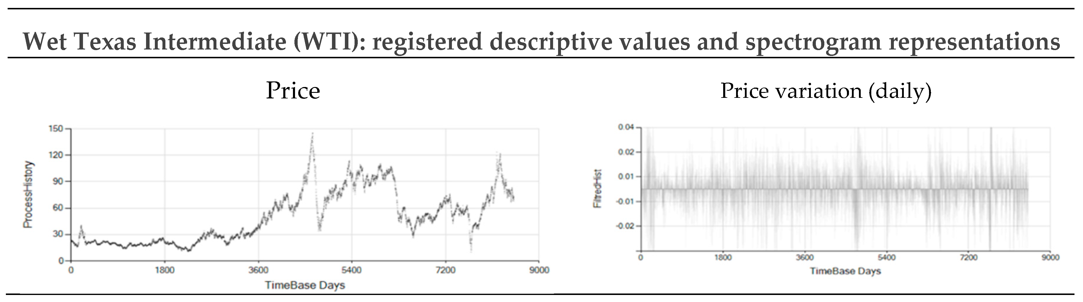
The repetition patterns detected for these market prices reveal characteristical differences among the stock market processes assessed. These processes’ fingerprints are visible in the space fraction occupied by repetitive sequences included in Figure 12, and the unfolded nested repeated sequences shown in Figure 13. Additionally, Figure 12 and Figure 13 show a tendency of the BTC price change to repeat shorter cycles of about ten days (represented by ten chars) than its counterparts GLD, SPX, and WTI, which exhibit cycles of nearly 30 days.
7. Results Summary and Discussion
The method functions on the base of the dimensionality reduction. Thus, we can think about the method as transforming a text object, whose dimensionality is of the order of the word diversity, into a lower-dimensional structure. The transformation follows a parameters set to define a specific process interpretation. Among the most relevant of these parameters are:
- : Discretization scale: Resolution (alphabet size). Scale’s non-linearity: Tangential, Hyperbolic, Linear.
- : Repetitions: Number of instances a sequence must appear to be considered a repeated sequence.
- : Text length. Text segment selected from the original full text.
The structure resulting from this transformación becomes the model we use to study the process by interpreting and representing it. In this document, we characterized three different types of time series: May's equation, Lorentz equations, and several stock market price evolutions in time. We obtained two representations for each process: the MSIR and the NPR. The method and its resulting representations potentially offer possibilities for further comparing processes' characteristics, extracting synthetic descriptions, and a better understanding of systems' behavior, thus providing ways to enhance data for modeling and projection purposes.
The MSIR's dimensionality equals the number of different sequences' lengths found. These sequences' lengths are the domain of graphs shown in Figure 7 (middle row), Figure 9, and Figure 11. Thus, each bubble in these graphs may represent several sequences. Therefore, the number of bubbles is considerably less than the number of sequences. The dimensionality of the counterpart representation, the NPR, equals the number of different sequences' lengths and the number of nesting depths found with the algorithm NESTED. The domain of graphs shown in Figure 8 (bottom row), Figure 11, and Figure 13 represent these sequences' lengths regarding the nesting level of each sequence. Consequently, NPR graphs exhibit a denser cloud of bubbles.
Despite the typical reaction to consider NPR graphs more complex, when graphical capabilities represent the nesting location of each symbol, the NPR shows more about the structure of the process modeled. The results about the complexity associated with the MSIR and NPR confirm this appreciation. Figure 14 illustrates the complexity reduction achieved if proper regard for nested patterns information and even redundancy. Thus, the NPC index is a promising figure for system comparison purposes. Its value comes from applying Expression (8). Nevertheless, Equation (8) is only feasible after the complete nested decomposition of the systems representing text.
An important observation in our results is the simultaneous noise and redundancy that emerges when working with NPR. Future studies should focus on applying the method to split fractions of information, noise, and redundancy.
8. Conclusions
The study introduces an algorithmic method for decomposing a unidimensional series of values into long, repeated sequences. The procedure simplifies the search space while keeping the text's structural essence, making the nested pattern detection computationally feasible.
The NRSLD is a valuable tool for characterizing long texts that may represent the behavior of unidimensional processes. The possibility of representing the tendency of specific sequence lengths to exist at certain nested depths may become, in later studies, an even more powerful tool to study and compare the system's structure and behavior. We believe these procedures are promising tools for characterizing and representing complex systems. By detecting the hidden nested structures within any complex system, we open up a way to quantify the nested complexity of systems and the redundancy of their descriptions.
Funding
No external funding was received for this research.
Conflicts of Interest
The author declares no conflicts of interest.
Appendix A
Appendix A.1. Pseudo Codes
Figure A11.
Pseudo-code of the Repeated sEquence eXtractor (REX) algorithm to search for repetitive symbol sequences within a long symbol string and form the set of symbols which constitutes the pattern of the interpretation.
Figure A11.
Pseudo-code of the Repeated sEquence eXtractor (REX) algorithm to search for repetitive symbol sequences within a long symbol string and form the set of symbols which constitutes the pattern of the interpretation.
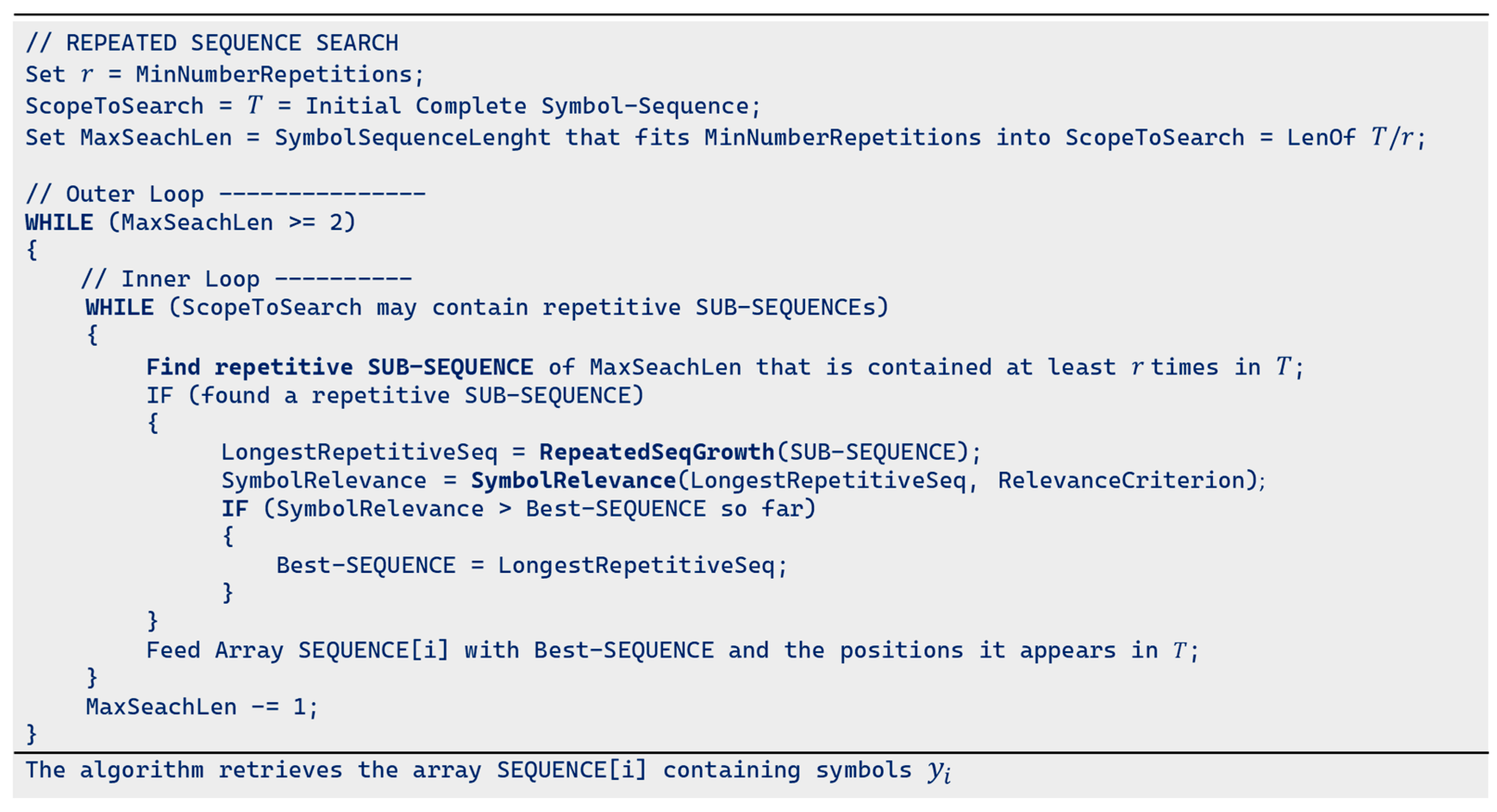
Figure A12.
Pseudo-code of the algorithm to implement the symbol-length growth mechanism.
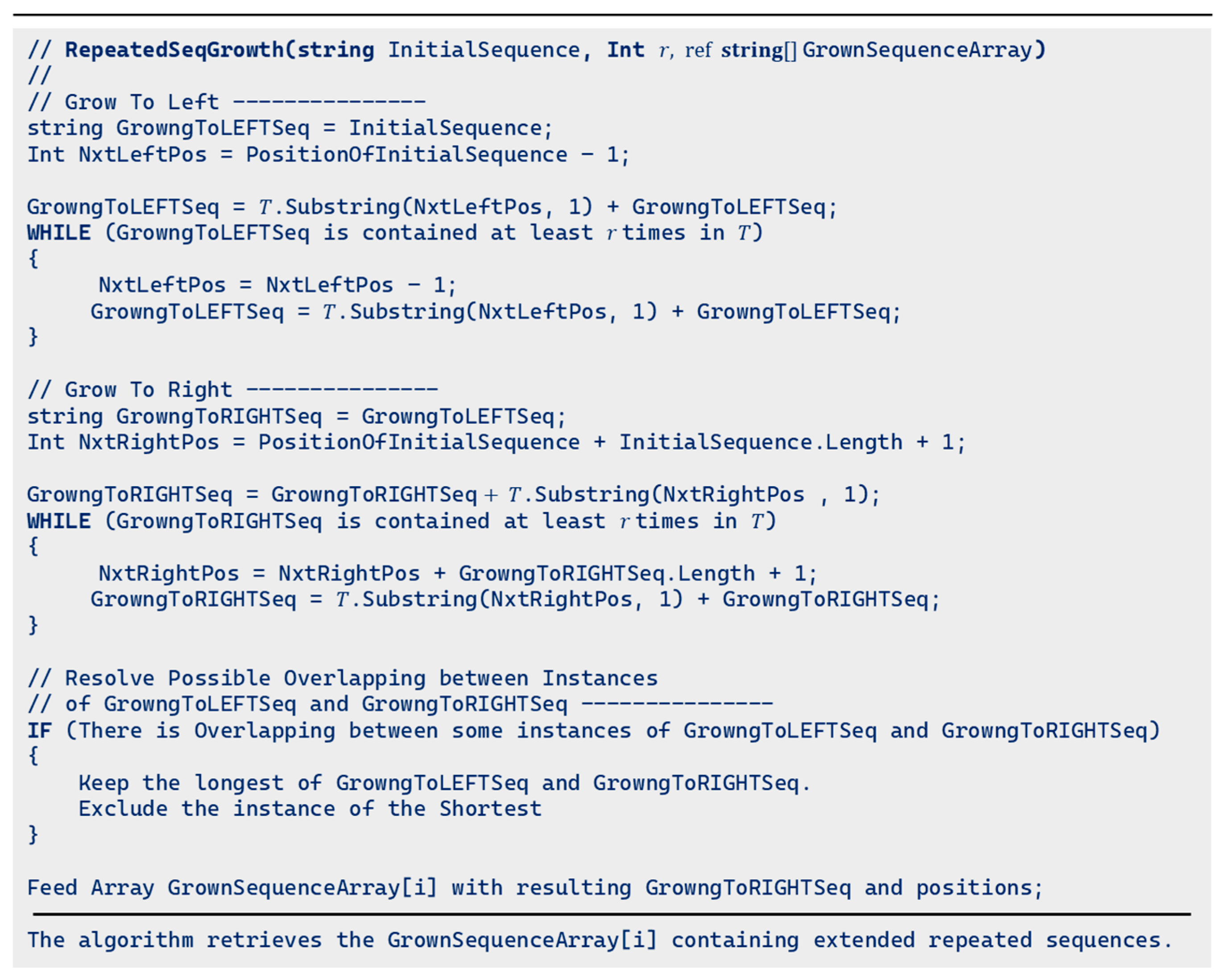
Figure A13.
Pseudo-code of the Nested Repeated Sequence Length Decomposition (NESTED) algorithm.
Appendix A.2. Stock Market Data
Figure A21.
Market GLD price and daily variations registered from 6756.10 $/Onz on 10/19/2012 (day 0) to 2563.99 on 6/1/2023 (day 2656).
Figure A21.
Market GLD price and daily variations registered from 6756.10 $/Onz on 10/19/2012 (day 0) to 2563.99 on 6/1/2023 (day 2656).
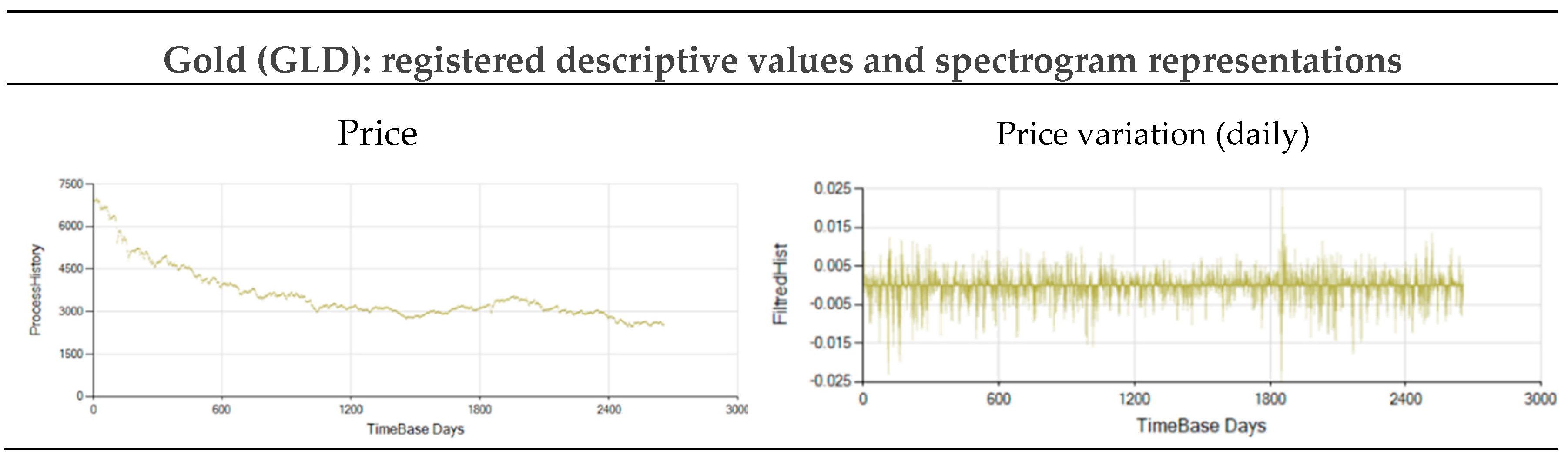
Figure A22.
Market BTC price and daily variations registered from 999.40 $ on 1/1/2017 (day 0) to 42315.00 on 12/26/2023 (day 2553).
Figure A22.
Market BTC price and daily variations registered from 999.40 $ on 1/1/2017 (day 0) to 42315.00 on 12/26/2023 (day 2553).
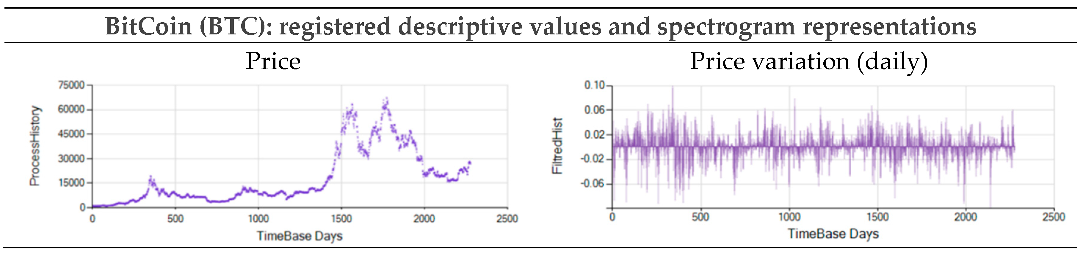
Figure A23.
Market SBX price and daily variations registered from 326.43 $ on 1/2/1991 (day 0) to 4221.02 on 6/1/2023 (day 8165).
Figure A23.
Market SBX price and daily variations registered from 326.43 $ on 1/2/1991 (day 0) to 4221.02 on 6/1/2023 (day 8165).
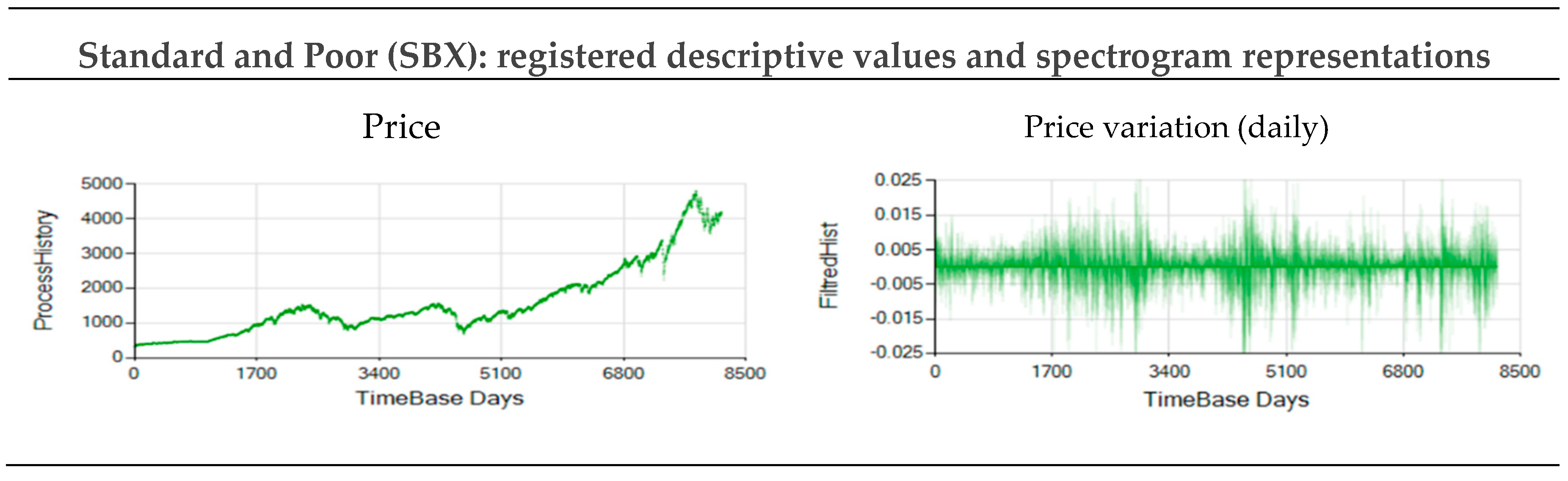
Figure A24.
Market WTI price and daily variations registered from 22.89 $/Brrl on 1/2/1990 (day 0) to 73.38 $/Brrl on 6/4/2023 (day 8516).
Figure A24.
Market WTI price and daily variations registered from 22.89 $/Brrl on 1/2/1990 (day 0) to 73.38 $/Brrl on 6/4/2023 (day 8516).
References
- Duin, R.P.W. The Origin of Patterns. Front Comput Sci 2021, 3, 1–16. [Google Scholar] [CrossRef]
- Huang, N.E.; Shen, Z.; Long, S.R.; Wu, M.C.; Snin, H.H.; Zheng, Q.; et al. The empirical mode decomposition and the Hubert spectrum for nonlinear and non-stationary time series analysis. Proc R Soc A Math Phys Eng Sci 1998, 454, 903–995. [Google Scholar] [CrossRef]
- Maheshwari, S.; Kumar, A. Empirical Mode Decomposition: Theory & Applications. Int J Electron Electr Eng 2014, 7, 873–878, Available: http://www.irphouse.com. [Google Scholar]
- Neill, D.B. Fast subset scan for spatial pattern detection. J R Stat Soc Ser B Stat Methodol 2012, 74, 337–360. [Google Scholar] [CrossRef]
- Febres, G.L. Basis to develop a platform for multiple-scale complex systems modeling and visualization: MoNet. J Multidiscip Res Rev 2019, 1. [Google Scholar] [CrossRef]
- Chioncel, C.P.; Gillich, N.; Tirian, G.O.; Ntakpe, J.L. Limits of the discrete fourier transform in exact identifying of the vibrations frequency. Rom J Acoust Vib 2015, 12, 16–19. [Google Scholar]
- Sayedi, E.R.; Sayedi, S.M. A structured review of sparse fast Fourier transform algorithms. Digit Signal Process 2022, 103403. [Google Scholar] [CrossRef]
- Febres, G.; Jaffe, K. A Fundamental Scale of Descriptions for Analyzing Information Content of Communication Systems. Entropy 2015, 17, 1606–1633. [Google Scholar] [CrossRef]
- Febres, G.L. A Proposal about the Meaning of Scale, Scope and Resolution in the Context of the Information Interpretation Process. Axioms 2018, 7, 11. [Google Scholar] [CrossRef]
- Rodríguez-Gironés, M.A.; Santamaría, L. A new algorithm to calculate the nestedness temperature of presence-absence matrices. J Biogeogr 2006, 33, 924–935. [Google Scholar] [CrossRef]
- Bar-Yam, Y. Multiscale Complexity/Entropy. Adv Complex Syst 2004, 07, 47–63. [Google Scholar] [CrossRef]
- Shannon, C.E. A mathematical theory of communication. Bell Syst Tech J 1948, 27, 379–423. [Google Scholar] [CrossRef]
- May, R.M. Simple mathematical models with very complicated dynamics. Nature 1976, 261. [Google Scholar] [CrossRef] [PubMed]
- Gershenson, C.; Kauffman, S.A.; Shmulevich, I. The Role of Redundancy in the Robustness of Random Boolean Networks. arXiv 2005, arXiv:nlin/0511018. [Google Scholar] [CrossRef]
- Kazantsev, E. Unstable periodic orbits and Attractor of the Lorenz. INRIA, 1998. [Google Scholar]
- Dong, H.; Zhong, B. The calculation process of the limit cycle for Lorenz system. Preprints 2021, 2021020419. [Google Scholar] [CrossRef]
Figure 1.
One-Scan repeated sequence length (OSRSL) probability graphs. Left: One-Scan repeated sequence probability envelope functions. Right: An explicit, graphic example of a One-Scan repeated sequence probability.
Figure 1.
One-Scan repeated sequence length (OSRSL) probability graphs. Left: One-Scan repeated sequence probability envelope functions. Right: An explicit, graphic example of a One-Scan repeated sequence probability.
Figure 2.
The Nested Repeated Sequence Length Decomposition (NRSLD). Left: Theoretical bands reflecting the place of different sequence lengths and repetitions for a 10000-char long text. Logarithmic scales represent the sequence length and the probability, or the space fraction the sequence length occupies in the text. Center: MSIR representation of the NRSLD of a 10000-char long text. The aligned points reflect sequences of lengths that appear the same number of times, disregarding the nesting depth where they appear within the text. Right: NPR representation of the NRSLD of a 10000-char long text. The nested depth of each sequence pattern expands the NP representation of the NRSLD. Smaller bubbles represent sequences found deeper nested into larger sequences located at a shallower depth.
Figure 3.
Repeated sequence searching strategy with two nested loops.
Figure 4.
Two interpretations of a unidimensional character sequence using symbol length and symbol frequency as criteria for pattern detection by successive selection of repetitive sub-sequences. The descriptions serve as syntactical representations of the characteristic patterns encountered in the text , and the corresponding structured pattern descriptions.
Figure 5.
Reference names of nodes in an NRSLD tree structure.
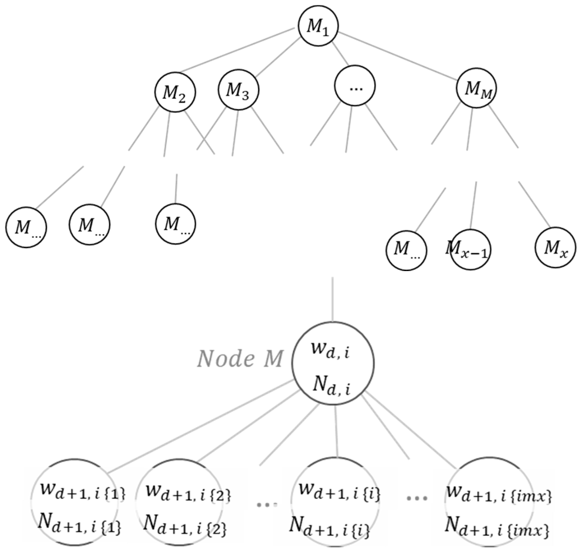
Figure 6.
Properly adjusted discrete scales can absorb the modeled series' non-linearity. Graphs 6a and 6b show a tangential discrete scale with resolution , extreme values = −1.5 and = 1.5, scale inflection point at , and parameter Graph (a) shows the Tangential Category Limits computed as a function of each possible value of the scale’s resolution applying Equations (10). Graph (b) shows the category discretely assigned to real series values in the horizontal axis. Graphs 6c and 6d show a hyperbolic discrete scale with resolution , extreme values = −1.5 and = 1.5, scale inflection point at , and parameter Graph (c) shows the Tangential Category Limits computed as a function of each possible value of the scale’s resolution applying Equations (11). Graph (d) shows the category discretely assigned to real series values in the horizontal axis. Graph (e) shows the spectrum of discretizing scales obtained by linearly combining the two former scales according to a weight σ.
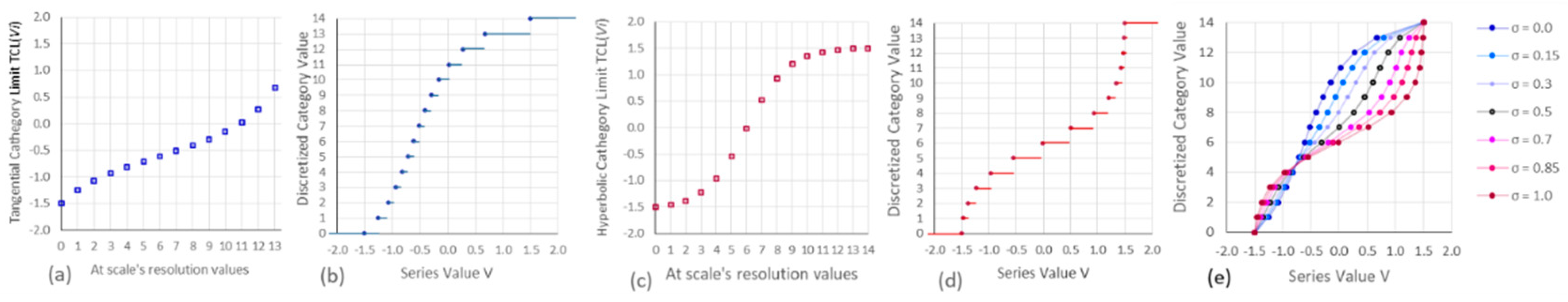
Figure 7.
Nested Sequence Decomposition and Interpretation general procedure steps.
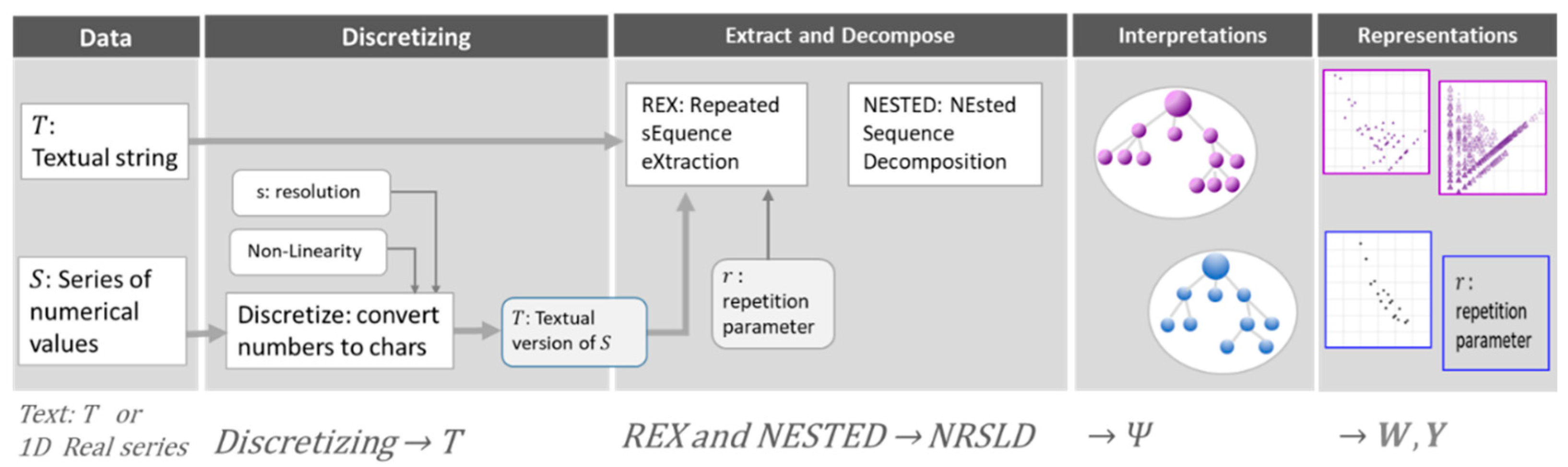
Figure 8.
The MSIR and NPR of May’s logistic Equation. Patterns detected for May’s logistic map are shown in the upper-left corner. The top graphs show the development of equation , for different parameter values , and . The bottom graphs show the corresponding Probability-Length decomposition, determined using the scale resolution and repetitions.
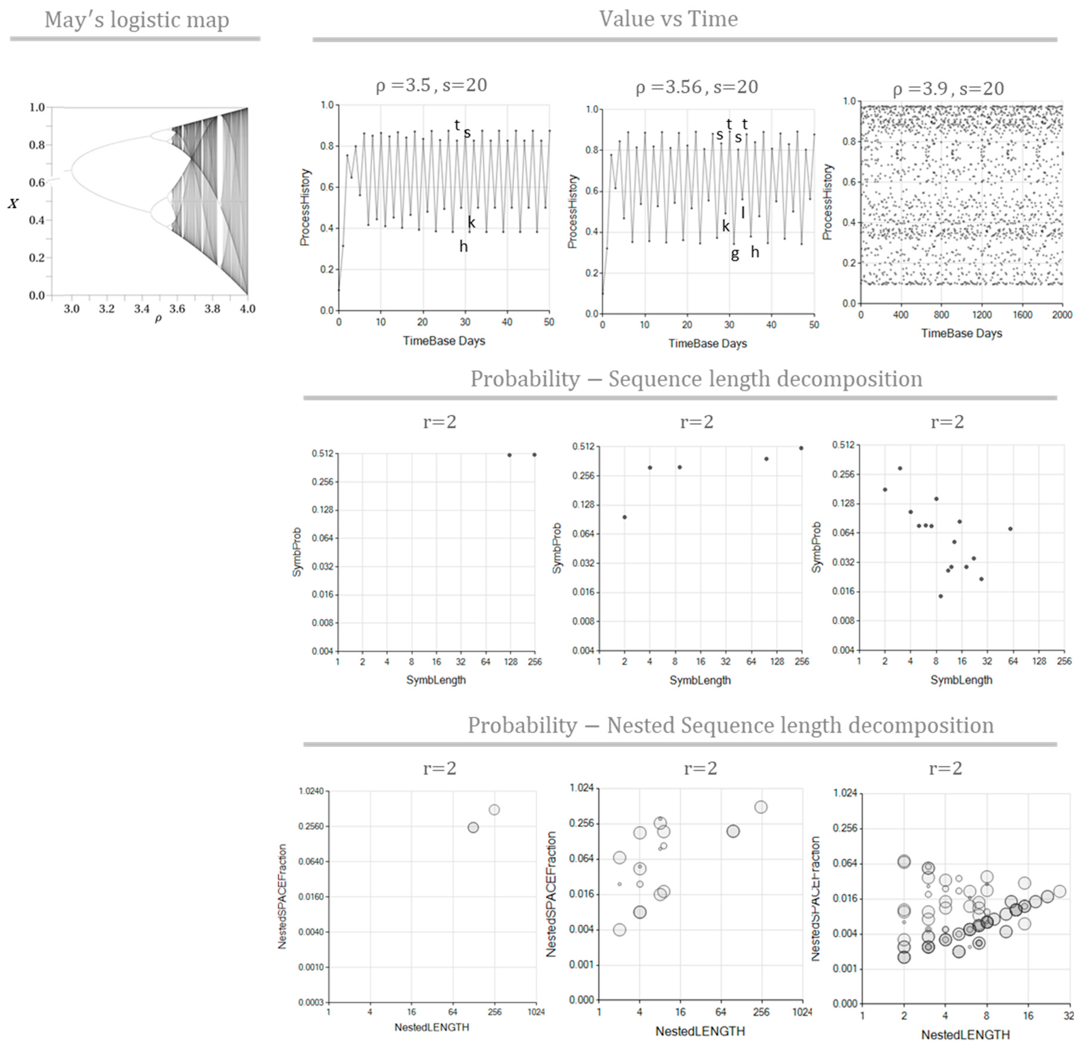
Figure 9.
Simulation of Lorentz equations represented in a three-dimensional space, and the process trajectory for each dimensional axis.
Figure 9.
Simulation of Lorentz equations represented in a three-dimensional space, and the process trajectory for each dimensional axis.
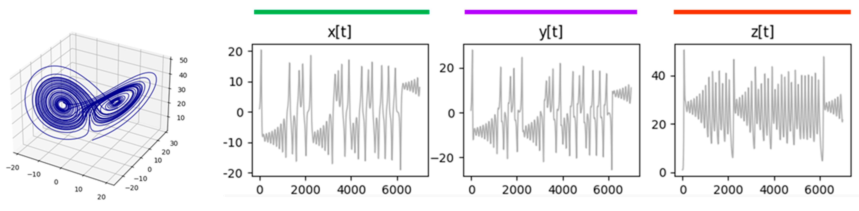
Figure 10.
The MSIR of the Lorentz Equations Process, simulated with 10000 time-steps (top), 20000 time-steps (middle), and 40000 time-steps (bottom), is characterized by the probability of repeating sequences as a function of the sequence length. The graphs show the sequence lengths probability distributions of the process described as , , and . Probability distributions are, green, violet, and red for , , and respectively.
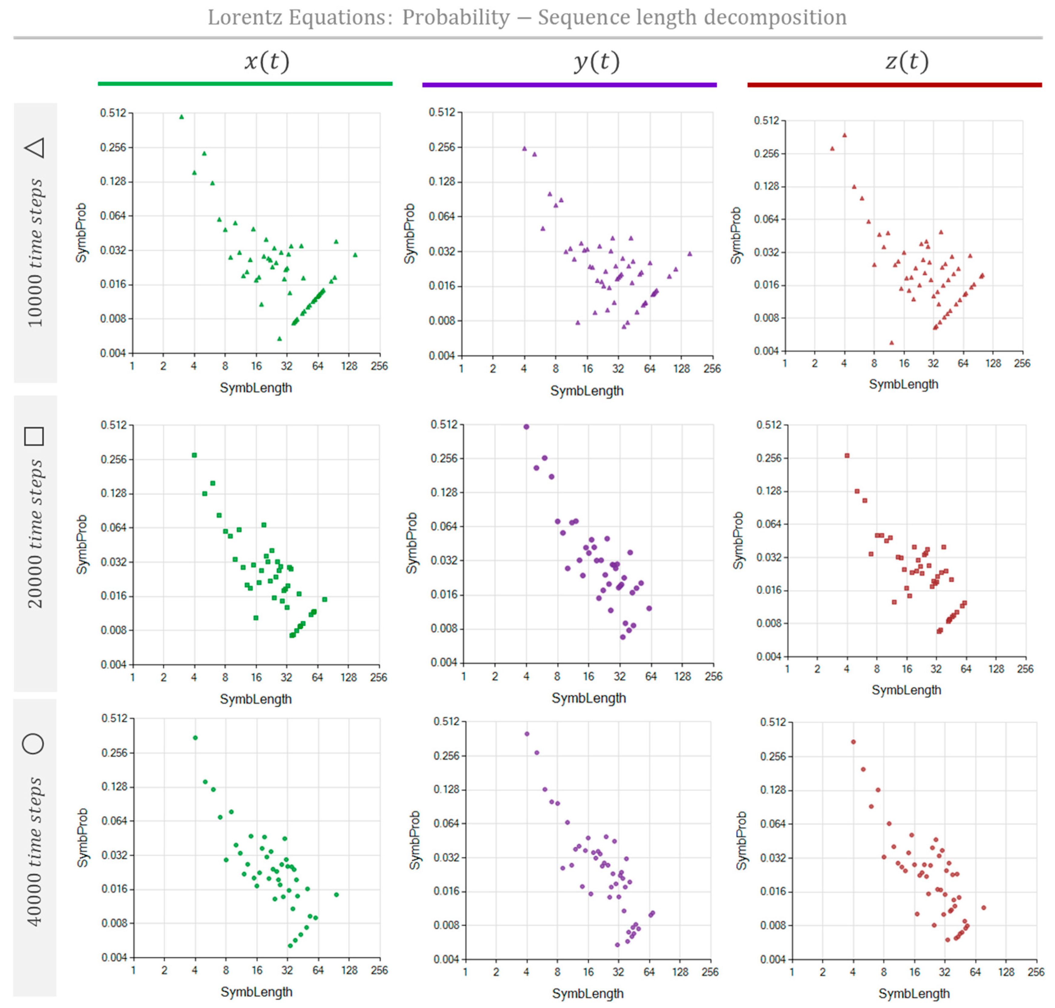
Figure 11.
The NPR of the Lorentz Equations Process, simulated with 10000 time-steps (top), 20000 time-steps (middle), and 40000 time-steps (bottom), is characterized by the probability of repeating sequences as a function of the sequence length. The graphs show the sequence lengths probability distributions of the process described as , , and . Probability distributions are green, violet, and red for , , and respectively.
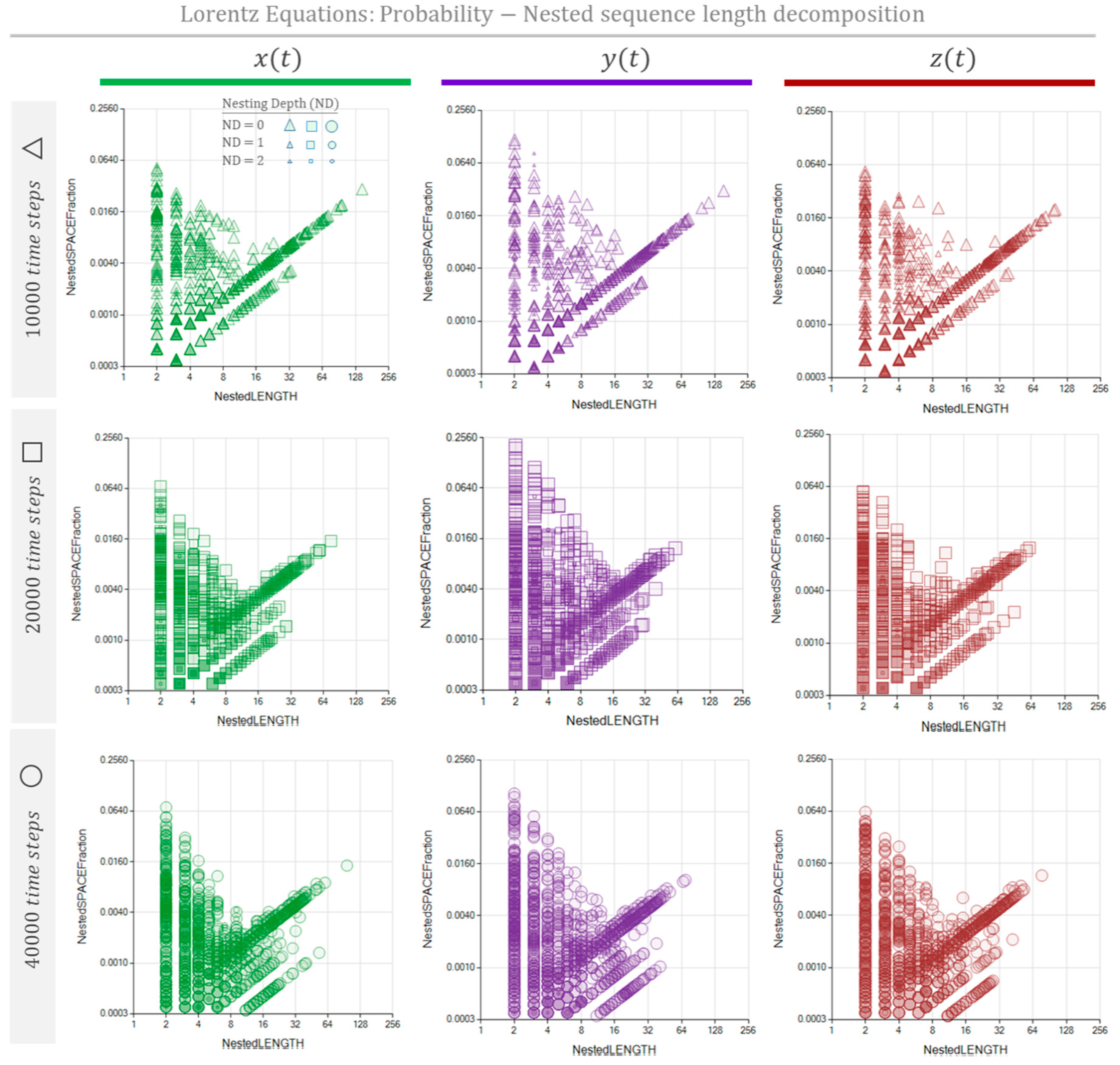
Figure 12.
The MSIR of several StockMarket indexes. Probability vs. sequence-length decomposition diagrams for four representative market time series: Gold (GLD), Standard and Poor Index (SPX), West Texas Intermediate (WTI), and BitCoin (BTC). Each diagram corresponds to the value daily change of the stock and was built with the scale and modeling conditions indicated in the left vertical bar next to each graph and Table 3.
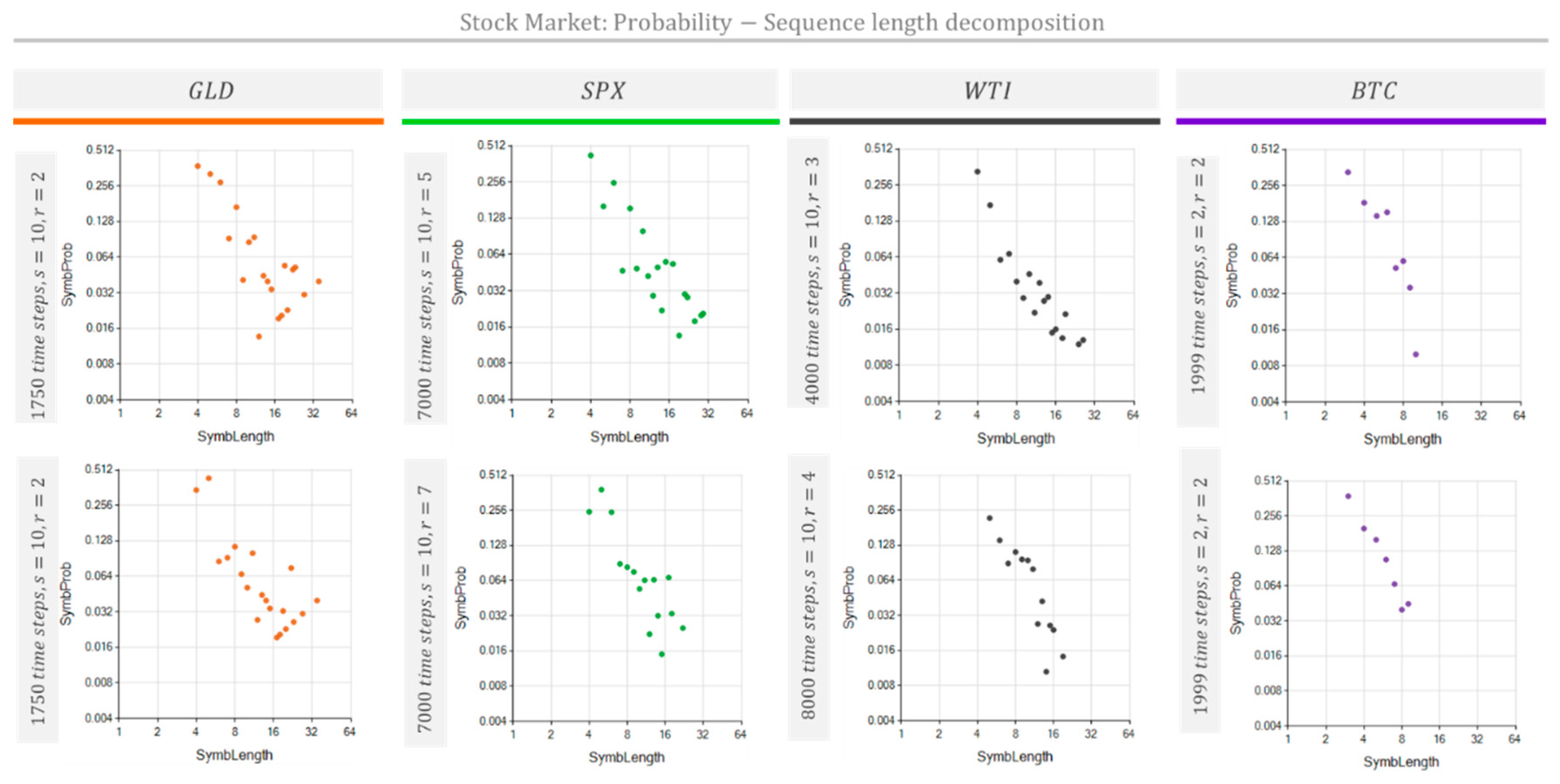
Figure 13.
The NPR of several StockMarket indexes. Probability vs. Nested sequence-length decomposition diagrams for four representative market time series: Gold (GLD), Standard and Poor Index (SPX), West Texas Intermediate (WTI), and BitCoin (BTC). Each decomposition diagram was built with the conditions indicated in the left vertical bar next to each graph.
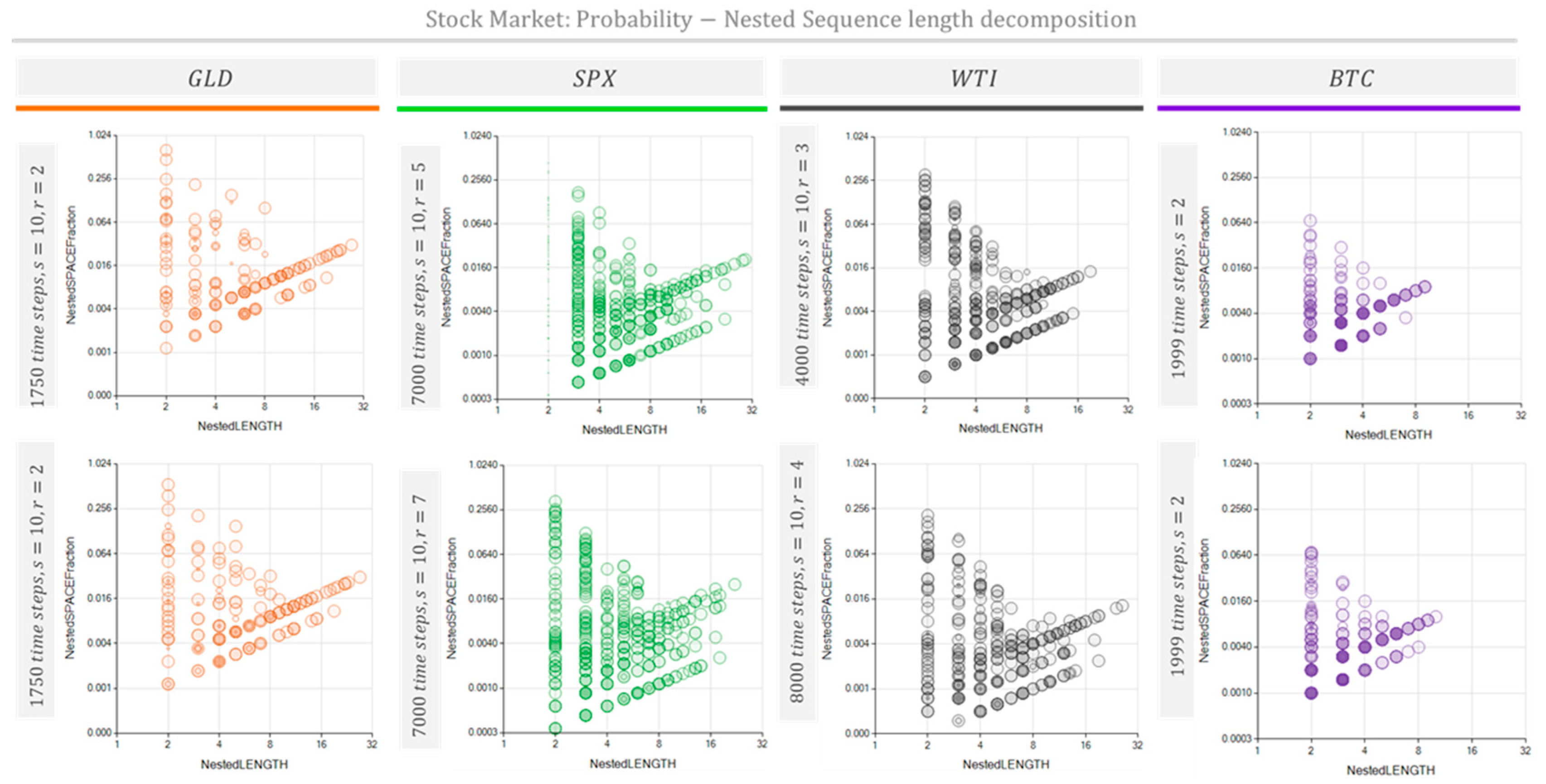
Figure 14.
Multiscale Complexity Index (MSIC) and Nested Complexity Index (NPC) comparison.


Table 1.
Pattern detection in May’s Logistic Map equation: parameters and results.
| Process | Scale: Type: Res/Inflect/Param | Sample length | : repetitions required | repetitions longest Symb. | Shortest/Longest repeated seq. | Complexity: MSIC/NPC | Shown in Figure 7 Row Col/Row Col |
|---|---|---|---|---|---|---|---|
| ρ = 3.5 | T: 20/10/0.01 | 1000 | 2 | 2 | 4/249 | 59.95/-5.00 | Cntr Left/Bttm Left |
| ρ = 3.56 | T: 20/10/0.01 | 1000 | 2 | 2 | 8/248 | NaN/-2.00 | Cntr Cntr/Bttm Cntr |
| ρ = 3.9 | T: 20/10/0.01 | 1000 | 2 | 2 | 548/548 | 32.99/9.06 | Cntr Rght/Bttm Right |
Table 2.
Pattern detection in Lorentz equations system: parameters and results.
| Process | Scale: Type: Res/Inflect/Param | Sample length | : repetitions required | repetitions longest Symb. | Longest sequence | Complexity: MSIC/NPC | Shown in Figure 9 and Figure 10 |
|---|---|---|---|---|---|---|---|
| Lorentz’s x(t) | T: 22/11/0.01 T: 22/11/0.01 T: 22/11/0.01 |
10000 20000 40000 |
2 4 6 |
2 4 6 |
145 75 96 |
128.09/16.28 597.93/20.11 1714.2/25.07 |
Green Top Green Middle Green Bottom |
| Lorentz’s y(t) | T: 22/11/0.01 T: 22/11/0.01 T: 22/11/0.01 |
10000 20000 40000 |
2 4 6 |
2 4 6 |
154 61 69 |
185.01/16.12 1397.77/20.17 2119.62/24.97 |
Violet Top Violet Middle Violet Bottom |
| Lorentz’s z(t) | T: 22/11/0.01 T: 22/11/0.01 T: 22/11/0.01 |
10000 20000 40000 |
2 4 6 |
2 4 6 |
100 62 77 |
165.19/16.60 638.60/19.75 1665.10/24.68 |
Red Top Red Middle Red Bottom |
Table 3.
Pattern detection in Stock Market time series: parameters and results.
| Process | Scale: Type: Res/Inflect/Param | Sample length | : repetitions required | repetitions longest Symb. | Longest sequence | Complexity: MSIC/NPC | Shown in Figure 11 and Figure 12 |
|---|---|---|---|---|---|---|---|
| Daily change of GLD price | T: 10/5/0.01 T: 10/5/0.01 |
1750 1750 |
2 2 |
2 2 |
35 35 |
171.88/9.39 133.51/8.93 |
Orange |
| Daily change of SPX index | T: 10/5/0.01 T: 10/5/0.01 |
7000 7000 |
5 7 |
5 8 |
29 22 |
1388.85/12.80 1864.81/11.34 |
Green |
| Daily change of WTI price | T: 10/5/0.01 T: 10/5/0.01 |
4000 8000 |
3 4 |
3 4 |
1926 | 1126.06/12.08 812.06/10.99 |
Black |
| Daily change of BTC value | T: 16/8/0.01 T: 16/8/0.01 |
1999 1999 |
2 2 |
2 2 |
9 10 |
277.96/10.61 244.68/10.65 |
Violet |
Disclaimer/Publisher’s Note: The statements, opinions and data contained in all publications are solely those of the individual author(s) and contributor(s) and not of MDPI and/or the editor(s). MDPI and/or the editor(s) disclaim responsibility for any injury to people or property resulting from any ideas, methods, instructions or products referred to in the content. |
© 2024 by the authors. Licensee MDPI, Basel, Switzerland. This article is an open access article distributed under the terms and conditions of the Creative Commons Attribution (CC BY) license (http://creativecommons.org/licenses/by/4.0/).
Copyright: This open access article is published under a Creative Commons CC BY 4.0 license, which permit the free download, distribution, and reuse, provided that the author and preprint are cited in any reuse.


