
Submitted:
13 June 2024
Posted:
17 June 2024
You are already at the latest version
Abstract
Recently, a significant number of tools for detecting dangerous objects have been developed. Unfortunately, the performance offered by them is overestimated due to the poor quality of the datasets used (insufficiently numerous, contain items not strictly related to dangerous objects, insufficient range of presentation conditions). To fill in a gap in this area we have built an extensive dataset dedicated to detecting the objects most often used in various acts of breaching public security (baseball bat, gun, knife, machete, rifle). This collection contains images presenting the detected objects with different quality and under different environmental conditions. We believe that the results obtained from it are more reliable and give a better idea of the detection accuracy that can be achieved under real conditions. We used the Faster R-CNN with different backbone networks in the study. The best results were obtained for the ResNet152 backbone. The mAP value was 85%, while the AP level ranged from 80% to 91%, depending on the item detected. An average real-time detection speed was 11-13 FPS. Both the accuracy and speed of the Faster R-CNN model allow it to be recommended for use in public security monitoring systems aimed at detecting potentially dangerous objects.
Keywords:
object detection
; faster R-CNN
; deep learning
; dangerous objects
; public safety
1. Introduction
In recent years, the problem of a growing number of incidents of violation of public security has become apparent. This is very well expressed by a statistic posted on the Statista website, showing the number of incidents involving active shooters in the United States between 2000 and 2022 (Figure 1a). It should be noted that such incidents have also occurred with other types of items (e.g., knives, machetes, baseball bats). Considering the type of weapon used in the aforementioned acts of violence, various types of firearms (guns, rifles, shotguns) dominate here, but knives and various types of cutting tools (e.g., machetes) are also present. Figure 1b shows the number robberies in the United States in 2022, by weapon used.
In a report titled A Study of Active Shooter Incidents in the United States Between 2000 and 2013, the FBI identified 7 locations where the public is most vulnerable to security incidents [1]. These locations include: open space, commercial areas, educational environments, residences, government properties, houses of worship, health care facilities. Figure 2 shows the number of active shooter incidents that occurred at the mentioned locations in the United States in 2022. The summary in Figure 2 does not include incidents involving other types of weapons, which also occurred. A potential opportunity to prevent acts of violence is provided by intelligent vision systems using surveillance cameras installed in public places. The images acquired by these cameras can be analysed for dangerous objects brought in by people. If such items are detected, the appropriate services (police, facility security, etc.) can be notified early enough. In this way, the chance can be increased to prevent a potential act of violence. Most public-use facilities (schools, train stations, stores, etc.) already use functioning monitoring systems, so the simplest and cheapest solution would be to integrate into these systems machine learning models trained to detect dangerous items in people. Great opportunities are offered here by deep convolutional neural networks, which are successfully used to detect various types of objects.
Among other applications, deep networks are used to automatically identify dangerous objects from X-ray images during airport security checks. Gao et al. proposed their own convolutional neural network model based on oversampling for detecting from an unbalanced dataset such objects as explosives, ammunition, guns and other weapons, sharp tools, pyrotechnics and others [3]. In contrast, Andriyanov used a modified version of the YOLOv5 network to detect ammunition, grenades and firearms in passengers’ main baggage and carry-on luggage [4]. In the proposed solution, the initial detection is carried out by the YOLO model, and the results obtained are subjected to final classification by the VGG-19 network. A number of models have also been developed for use in monitoring systems for public places. Gawade et al. used a convolutional neural network to build a system designed to detect knives, small arms and long weapons. The accuracy of the built model was 85% [5]. The convolutional neural network ensemble was also applied by Haribharathi et al. [6]. It has achieved better results than single neural networks during automatic weapon detection. In addition to convolutional neural networks, YOLO and Faster R-CNNs are often used. Kambhatla et al. conducted a study on automatic detection of pistol, knife, revolver and rifle using YOLOv5 and Faster R-CNN networks [7]. In contrast, Jain et al. used SSD and Faster R-CNN networks for automatic gun detection [8]. Some authors propose their own original algorithms. One example is the PELSF-DCNN algorithm for detecting guns, knives and grenades [9]. According to the authors, the accuracy of their method is 97.5% and exceeds that of other algorithms. A novel system for automatic detection of handguns in video footage for surveillance and control purposes is also presented in [10]. The best results there were obtained for a model based on Faster R-CNN trained on its own database. The authors report that in 27 out of 30 scenes, the model successfully activates the alarm after five consecutive positive signals with an interval of less than 0.2 seconds. In contrast, Jang et al. proposed autonomous detection of dangerous situations in CCTV scenes using a deep learning model with relational inference [11]. The authors defined a baseball bat, a knife, a gun and a rifle as dangerous objects. The proposed method detects the objects and, based on relational inference, determines the degree of danger of the situations recorded by the cameras. Research on detecting dangerous objects is also being undertaken to protect critical infrastructure. Azarov et al. analysed existing real-time machine learning algorithms and selected the optimal algorithm for protecting people and critical infrastructure in large-scale hybrid warfare [12].
One of the challenges in object detection is the detector’s ability to distinguish small objects during hand manipulation. Pérez-Hernández et al. proposed improving the accuracy and reliability of detecting such objects using a two-level technique [13]. The first level selects proposals for regions of interest, and the second level uses One-Versus-All or One-Versus-One binary classification. The authors created their own dataset (gun, knife, smartphone, banknote, purse, payment card) and focused on detecting weapons that can be confused by the detector with other objects. Another problem is the detection of metal weapons in video footage. This is difficult because the reflection of light from the surface of such objects results in a blurring of their shapes in the image. As a result, it may be impossible to detect the objects. Castillo et al. developed an automatic model for detecting cold steel weapons in video images using convolutional neural networks [14]. The robustness of this model to illumination conditions was enhanced using so-called brightness-controlled preprocessing (DaCoLT) involving dimming and changing the contrast of the images during the learning and testing stages. The authors of an interesting paper in the field of dangerous object detection are Yadav et al. [15]. They made a systematic review of datasets and traditional and deep learning methods that are used for weapon detection. The authors highlighted the problem of identifying the specific type of firearm used in an attack (so-called intra-class detection). The paper also compares the strengths and weaknesses of existing algorithms using classical and deep machine learning methods used to detect different types of weapons.
Most of the available results in the area of object detection relate to datasets containing different categories of objects that are not strictly focused on the problem of detecting dangerous objects. In addition, the results presented are overestimated because a significant portion of the images in the collections used to build and test the models represent the objects themselves to be detected. They are not in the hand of any person, are large enough and perfectly visible. Consequently, the detector has little problem detecting such objects correctly and the reported detection precision is high. Such an approach misses the purpose of the research, which is to detect objects in the hands of people (potential attackers). Such objects are usually smaller, partially obscured and less visible, making them more challenging for the detector.
Against this background, our research stands out because it provides an insight into the construction of an object detector using a more specialised data set, which increases the trustworthiness and significance of the results obtained. We prepared the dataset in such a way that it contains items that are most often applied in acts of violence and violation of public safety, these are: baseball bat, gun, knife, machete and rifle. So, we can say that we have built and used a dataset dedicated to the task of detecting potentially dangerous objects. It is also important that objects are presented with different quality, namely: clearly visible, partially obscured, small (longer viewing distance), blurred (worse sharpness) and poorly lit. As a result, the dataset better reflects real-world conditions and the results obtained are more trustworthiness. The dataset we have prepared is publicly available to a wide range of researchers who are potentially interested in using it in own research. An additional contribution of our work is to show the possibility of using the popular Faster R-CNN architecture to detect dangerous objects by public place monitoring systems. The conducted experiments have shown that this kind of detector is characterized by low hardware requirements and high accuracy, which allows it to be recommended for the same or similar applications as those included in the subject of our research.
Section 2 briefly describes the Faster R-CNN used and characterises the object detection quality measures used and how the dataset was prepared. Section 3 contains the results of the training and evaluation processes. Section 4 evaluates the results obtained and compares them with the results of other authors. It also describes the effects of testing the best model using a webcam. The entire work ends with a summary and conclusions in Section 5.
2. Materials and Methods
The purpose of the research the results of which are presented in this paper was to build a model suitable for use in monitoring systems for public places. The objects monitored by such systems are usually people who move relatively slowly within the observed area. Therefore, the frequently used operating speed of such systems, amounting to several FPS, is quite sufficient. Taking this into account, the basic requirement for the model was high accuracy in detecting objects, especially small objects. The assumption made in the study was that the model would detect a specific set of potentially dangerous objects, such as baseball bat, gun, knife, machete, rifle. Comparing the size of these objects with the size of the monitored scene, there is no doubt that they are small objects, occupying a negligible portion of the image frame. Taking into account the requirements formulated earlier, the Faster R-CNN was chosen. This was due to the fact that, on the one hand, this type of network copes well with the detection of small objects, and on the other hand, it allows to achieve a processing speed of several dozen FPS, which is sufficient for use in monitoring systems.
2.1. Faster R-CNN
The genesis of the Faster R-CNN is related to the development of the R-CNN by R. Girshick et al. [16]. This network offered higher accuracy compared to previous traditional object detection methods, but its main drawback was its low speed. For each image, the R-CNN generated approximately 2000 region proposals of various sizes, which were then subjected to feature extraction using a convolutional network [17,18,19]. In 2015, R. Girshick proposed to improve the R-CNN and introduced a new network called Fast R-CNN [20]. Instead of extracting features independently for each ROI, this type of network aggregated them in a single analysis of the entire image. In other words, the ROIs belonging to the same image shared computation and working memory. The Fast R-CNN detector proved to be more accurate and faster than previous solutions, but it still relied on the traditional method of generating 2000 region proposals (Selective Search method), which was a time-consuming process [21].
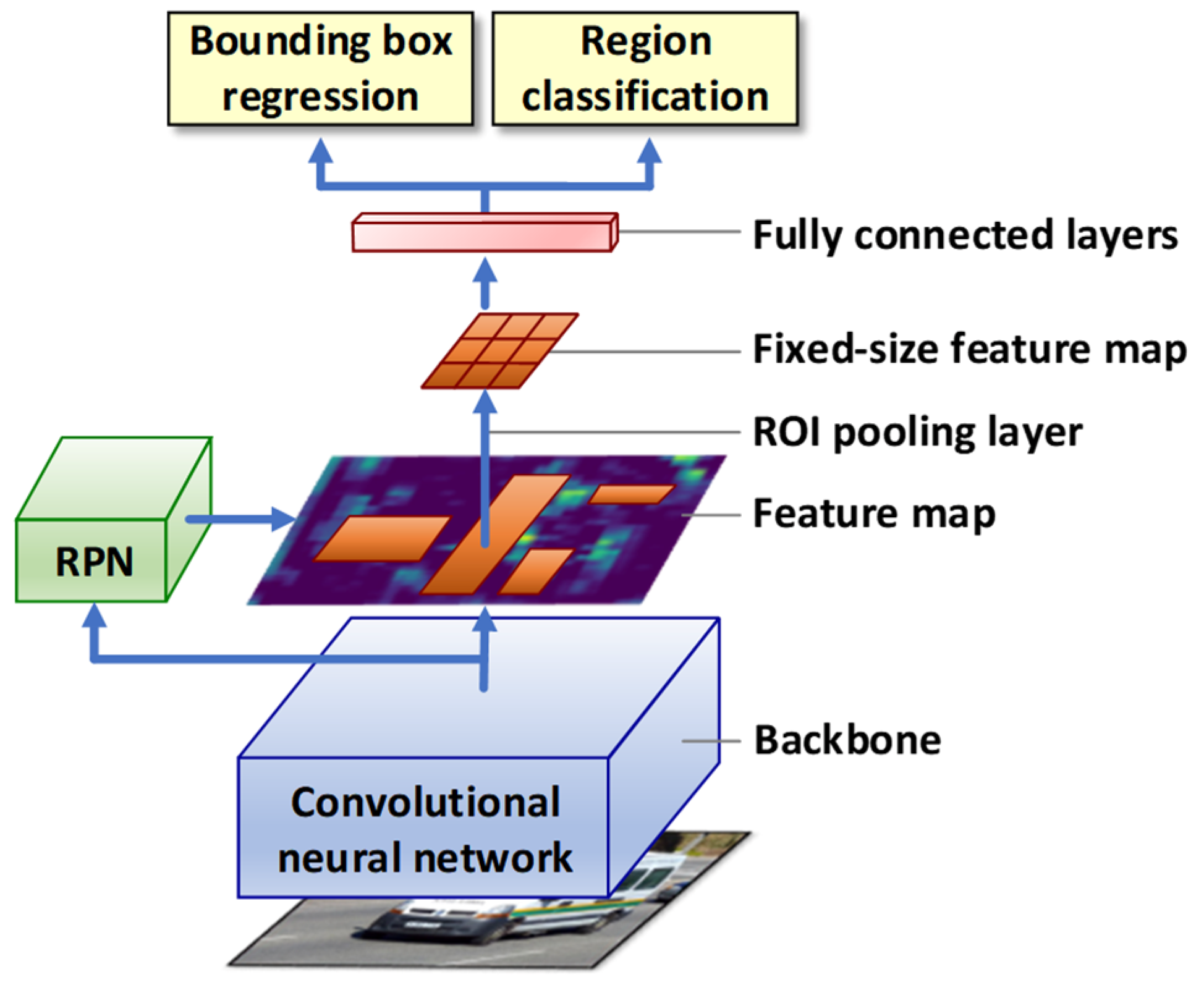
The problem of the temporal efficiency of the Fast R-CNN was the reason for the development of a new detector called Faster R-CNN by S. Ren et al. [22] It improved the detection speed of Fast R-CNN by replacing the previously used Selective Search method with a convolutional network known as a Region Proposal Network (RPN). Figure 3 shows the architecture of the Faster R-CNN detector, and its operation can be described as follows:
- A convolutional neural network takes an input image and generates a map of image features on its output.
- The feature map is passed to the input of the RPN attached to the final convolutional backbone layer. The RPN acts as an attention mechanism for Fast R-CNNs. It tells you which region to look out for in relation to the potential presence of the object.
- The feature map is then passed to the ROI pooling layer to generate a new map with a fixed size.
- At the end of the process, the fully connected layers perform a region classification and a regression of the bounding box position.
Figure 3.
Faster R-CNN [22].
Figure 3.
Faster R-CNN [22].
The RPN takes input from a pre-trained convolutional network (e.g., VGG-16) and outputs multiple region proposals and predicted class labels for each of them. Region proposals are bounding boxes based on predefined shapes that are designed to speed up the region proposal operation. In addition, a binary prediction is used, indicating the presence of an object in a given region (the so-called objectness of the proposed region) or its absence. Both networks (RPN and backbone) are trained alternately, which allows you to tune parameters for both tasks at the same time. The introduction of the RPN has significantly reduced the number of regions proposed for further processing. This number was no longer equal to 2000, as in the case of Fast R-CNN, but was several hundred, depending on the complexity of the input images. This directly reduced training and prediction times and enabled the Faster R-CNN detector to be used in near real time.
2.2. Assessing the Quality of Object Detectors
Most indexes for assessing the quality of object detection are based on two key concepts, these are prediction confidence and Intersection over Union (IoU). Prediction confidence is a probability estimated by a classifier that a predicted bounding box contains an object. IoU, on the other hand, is a measure based on the Jaccard index that evaluates the overlap between two bounding boxes—the predicted (Bp) and the ground-truth (Bgt). With IoU, it is possible to determine whether the detection is correct or not. The measure is the area of overlap between the predicted and ground-truth frames divided by the area corresponding to the sum of the two frames (Figure 4).
Prediction confidence and IoU are used as criteria for determining whether object detection is true positive or false positive. Based on these, the following detection results can be determined:
True Positive (TP). A detection is considered true positive when it meets three conditions:
- the prediction confidence is greater than the accepted detection threshold (e.g., 0.5);
- the predicted class is the same as the class corresponding to the ground-truth box;
- the predicted bounding box has an IoU value greater than the detection threshold.
Depending on the metric, the detection threshold is usually set to 50%, 75% or 95%.
False Positive (FP). This is a false detection and occurs when either of the last two conditions is not met.
False Negative (FN). This situation occurs when the prediction confidence is lower than the detection threshold (no ground-truth box detected).
True Negative (TN). This result is not used. During object detection, there are many possible bounding boxes that should not be detected in the image. So, a TN value would mean all possible bounding boxes that were not correctly detected (there are a lot of them in the image).
The detection results allow calculating the values of 2 key quality measures, which are precision and sensitivity. Precision is an ability of the model to detect only correct objects. It is a ratio of the number of true positive (correct) predictions to the number of all predictions (1):
Recall determines the model’s ability to detect all valid objects (all ground-truth boxes). It is a ratio of the number of true positive (correct) predictions to the number of all ground-truth boxes (2):
Precision-recall curve. One way to evaluate the performance of an object detector is to change the level of detection confidence and plot a precision-recall curve for each class of objects. An object detector of a certain class is considered good if its precision remains high as the recall increases. This means that if the detection confidence threshold changes, the precision and recall will still remain high. Put a little differently, a good object detector detects only the right objects (no false-positive predictions means high precision) and detects all ground-truth boxes (no false-negative predictions means high recall).
Average precision. Precision-recall curves often have a zigzag course, running up and down and intersecting each other. Consequently, comparing curves belonging to different detectors on a single graph becomes a difficult task. Therefore, it is helpful to have an average precision (AP), which is calculated by averaging the precision values corresponding to sensitivities varying between 0 and 1. The average precision is calculated separately for each class. There are 2 approaches to calculating average precision. The first involves interpolating 11 equally spaced points. The second approach, introduced in the 2010 PASCAL VOC competition, involves interpolating all data points. The average precision is calculated for a specific IoU threshold, such as 0.5, 0.75, etc.
The 11-point interpolation approximates the precision-recall curve by averaging the precision for a set of 11 equally spaced recall levels [0, 0.1, 0.2, ..., 1] (3):
where the interpolated precision at a specific recall level r is defined as the maximum precision occurring for the recall level (4):
In the second method, instead of interpolation based on 11 equally spaced points, interpolation for all points is used (6):
where are the recall levels (in ascending order) at which the precision is interpolated.
Mean AP. Average precision covers only one class, while object detection mostly involves multiple classes. Therefore, mean average precision (mAP) is used for all K classes (6):
Inference time. Inference time is a time it takes for a trained model to make a prediction of new, previously unknown data on a single image. When detecting objects in video sequences, in addition to inference time, a second parameter is often used, namely the frame rate per second (FPS). This parameter indicates the frequency at which inference is performed for successive frames of the video stream. The choice of object detection model depends on the specific requirements of the application. Some of them favour accuracy over speed (as in our research), while others prefer faster processing, especially in real-time applications. Consequently, researchers and developers often use FPS as a critical factor when deciding which model to implement for a particular use case. Be aware that the FPS value depends on the inference time, but also on the duration of additional operations, such as image capture, pre-processing, post-processing, displaying the results on the screen, etc... The values of inference time and FPS depend on the architecture of the model and the hardware/software platform on which the model was run.
2.3. Preparing the Dataset
The dataset used did not come from a single, well-defined repository. It was prepared specifically for the research conducted. In order to gather it, a search was made through a number of sources available on the Internet, offering free access to the collected resources. An important issue during the search for images was that they should cover different situations and different conditions of image acquisition by surveillance cameras installed in public places. Accordingly, the following categories of images can be distinguished in the collected dataset (Figure 5): objects clearly visible, objects partially covered, small objects, poor objects sharpness, and poor objects illumination. During the image search, care was taken to ensure that the collected dataset was balanced, that is, that a similar number of classes of detected objects (baseball bat, gun, knife, machete, rifle) was maintained.
As part of the image’s preparation for the study, they were scaled (and cropped where necessary) so that the smaller side was no shorter than 600 pixels and the larger one was no longer than 1,000 pixels. This operation was conditioned by the requirements of the Faster R-CNN. The next stage of data preparation was image labelling. This activity consisted of marking the detected objects on the images using bounding boxes. Label Studio was used for this purpose [23]. The image annotations were saved in the Pacal VOC format, according to which the description about each image is included in the corresponding XML file.
The full dataset contained 4,000 images. This set was randomly divided into training set (75% of the full set) and test set (25% of the full set). As a result, the training set contained 3,000 images, and the test set—1,000. Figure 6 details the number of detected objects in each of the aforementioned sets.
3. Results
3.1. Training Process
During training, 5 architectures of the pre-trained backbone networks were used: ResNet50, ResNet101, ResNet152 and 2 VGG-16 networks differing in the pre-trained weights (VGG-16 Caffe and VGG-16 Pytorch). During the model’s construction stage, 30 training epochs were used. While the first 15 epochs, the learning rate was 10-3, and during the next 15 epochs its value was 10-4. After each epoch, the mean average precision (mAP) of the model was calculated based on the test set. At the same time, the weights obtained in a given epoch were saved, so it was possible to select the best set of weights after the entire training process was completed. Table 1 collects the values of the more important hyperparameters used in the training process.
The images belonging to the training set were characterized by a great diversity. The detected objects were presented at different size scales, with different angles of rotation and different horizontal and vertical displacement within the image frame. In addition, the images were characterized by different levels of sharpness and brightness, and some of the detected objects were partially covered by other objects. Given these features and a relatively large number of objects belonging to each class, additional augmentation was abandoned at the model training stage. The results of the training are presented in Figure 7. The loss plots of the RPN, object detector, as well as the total loss and mAP values show that the 30 training epochs that were used were enough to achieve convergence of the training algorithm for each of the backbone network used.
A computer with Windows 11 64-bit operating system, Intel Core i7-12650H 2.70 GHz processor and 32 GB RAM was used to train the models. PyTorch 2.1.2 platform and the Python 3.10 programming language were employed. Calculations were performed using the GPU (NVIDIA GeForce RTX 3060 Laptop GPU, 6 GB GDDR6), the CUDA 11.8 platform and the cuDNN 8.9.6 library. Table 2 shows the total training time of each of the five models built.
3.1. Model Evaluation
Based on the test set, 5 models differing in backbone network were evaluated. The test set was balanced, as was the full dataset. The percentage of each object class in it was about 20% (Figure 6c). Figure 8 shows precision-recall plots for each object category. The performance of a given model is better the longer a high precision value is maintained with an increasing recall value. In the graph, this is manifested in such a way that the precision-recall curve runs closer to the point with coordinates (1, 1). The graphs shown in Figure 8 indicate that when detecting baseball bat, knife and machete, the best performance was achieved by models based on ResNet101 and Resnet152. In contrast, for gun and rifle, the model based on ResNet152 was the best.
Figure 9 shows bar graphs reflecting the average precision of detection of different object categories by each model. The gun was detected with the highest precision by ResNet152 (AP0.5 = 91.3%). The same object was detected with slightly lower precision by ResNet101 (AP0.5 = 89.7%). Third place went to gun detection accuracy by ResNet50 (AP0.5 = 89.5%). The worst results were for a machete detected by VGG16_PyTorch (AP0.5 = 68.5%) and a knife detected by VGG16_PyTorch (AP0.5 = 68.3%).
Bar graphs showing the value of the mean average precision of detection of all 5 object classes are shown in Figure 10. The best result was achieved by ResNet152 (mAP = 85%), a slightly worse mAP value (84.5%) was achieved by ResNet101. The average precision of the other models was: 81.8% (ResNet50), 78.3% (VGG16_Caffe) and 77.4% (VGG16_PyTorch).
Model evaluation was performed on the same computer as the network training (computer specifications are given in Section 2.5). The average inference time per image frame ranged from 74 ms for VGG-16_Caffe and VGG-16_Pytorch to 101 ms for ResNet152, depending on the topological depth of the backbone network used (Figure 11).
4. Discussion
4.1. Assessment of the Results Obtained
Figure 12 shows an example of the results obtained using the ResNet152 model. The analysed images could be divided into several categories, depending on the presentation of the detected objects.
The first category included images with objects that were clearly visible (Figure 12a), which were detected with 100% accuracy, regardless of their size. Objects that were partially hidden in the hand (gun, knife) or partially obscured by body parts of the subject were detected with similar accuracy (Figure 12b). In the images belonging to the third category, the detected objects were presented on a smaller scale because they were further away from the camera (Figure 12c). Again, the model did very well in detecting them, as shown by the predicted bounding boxes in red. The next type of images had poorer sharpness, as a result of which the detected objects were less clear than in the other images (Figure 12d). Detection confidence here was not 100%, as for the previous categories of images. There were also greater differences in localization between the predicted bounding boxes and the ground-truth boxes. However, despite the more difficult conditions, the model performed very well in detecting all classes of objects. In most cases, detection confidence exceeded 90%. The last category of images presented the detected objects in poorer lighting, resulting in darker images and less visible objects (Figure 12e). Despite the more difficult conditions, the model easily detected objects that were faintly visible, small (gun, knife) and at a greater distance from the camera. The results showed that the advantage of the built model was that it was highly effective in detecting objects, regardless of the conditions of their presentation, such as the sharpness and brightness of the image, the size of the objects or their partial obscuration by other objects.
In order to carry out more accurate diagnostics of the model, a confusion matrix was constructed (Figure 13a). It allows us to determine the type and number of errors made by the model. The most errors were made for knives and machetes. When detecting these items, 14 knives were recognized as machetes and 15 machetes were classified as knives. In this case, there were a number of images showing long knives and short machetes, which could pose a challenge for the detector. The confusion matrix also included cases where objects were detected when they were not actually present in the image (false positives) and cases where existing objects were not detected (false negatives). The number of false-positive cases was 112, while the number of false-negative cases was much lower at 37. The highest number of false detections was observed for knives (32), machetes (27) and rifles (22). In order to reduce the number of such false detections, the number of training cases will be increased in the course of further research, and augmentation will be used, which was abandoned in the present study. The confusion matrix also made it possible to calculate the recall of the model. The value of this parameter was as follows: baseball bat—95.3%, gun—94.6%, knife—90.0%, machete—85.5%, rifle—88.5% (Figure 13b).
4.2. Comparison of Results with Those of Other Authors
Table 3 summarises the dangerous object detection results obtained by different authors using the Faster R-CNN. Unfortunately, for various reasons, it is difficult to compare our results with them. Other authors have used different datasets in their studies. Some of them are available on the Internet, while others were prepared specifically for the research in progress. In turn, the images used in the experiments varied in terms of size, type (photographs, video) and presentation of the objects detected (objects occupying the entire surface of the image and objects presented in real life—held in a person’s hand). Different measures of performance were also used (accuracy, AP, mAP, F1-score and others). However, the most commonly used measures were precision, mAP, recall and mAR with a standard IoU threshold of 0.50. We have therefore used the aforementioned measures in the summary in Table 3.
The largest number of results available relates to gun detection, as this is the most commonly used weapon in assaults and acts of violence, according to statistics. The precision value we obtained in this case (AP = 91.3%) is in second place. The best precision for gun detection was obtained by Vijayakumar et al.—this was 96.6% [24]. Regarding the recall of gun detection, the best result (AR = 100%) was obtained by Olmos et al. [10] and González et al. [27]. Our result, with AR = 94.6%, is in second place. Far fewer results are available for the detection of knives and rifles. Our obtained rifle detection precision of 85.3% is second best in the presented list. The best precision (AP = 100%) was obtained by Vijayakumar et al. [24]. In contrast, the highest recall of rifle detection (AR = 96%) was also obtained by Vijayakumar et al. [24]. In our study, an AR=88.5% was achieved for rifles. By far the highest detection precision was obtained for knives. Our result, equal to 80.8%, far exceeds the results of other authors, who obtained AP = 55.8% (Vijayakumar et al. [24]) and AP = 46.7% (Fernandez-Carrobles et al. [29]). The knife detection recall we obtained was 90.0%. The best result obtained by other authors in this case was 52% (Vijayakumar et al. [24]). However, it was not possible to find research results on the use of the Faster R-CNN for the detection of baseball bats and machetes. This demonstrates the unique nature of the dataset used in the study and the results obtained. In terms of average precision and average sensitivity for detecting a set of different objects, our results were the highest (mAP = 85%, mAR = 90.6%).
4.3. Application of the Results Obtained to the Prediction of New Images
The model that proved most effective at the evaluation stage (ResNet152) was selected for further testing involving image prediction using the camera. The experiments used the same computer used for model training and evaluation, and a Tracer HD WEB008 webcam acting as a surveillance camera. The scenario of the experiment involved monitoring people entering the room and detecting potentially dangerous objects in them. Both the distance of the camera from the entrance door and its installation height were 2.5 meters. Figure 14 shows selected frames of the recorded image. During recording, the frames were scaled to 800×600 pixels so as to meet the Faster R-CNN model’s minimum input image size requirements. At this resolution, the average processing speed was 11 to 13 FPS. Such a speed is sufficient for use in public space surveillance systems, where the typical processing speed of image frames is usually a dozen FPS. During the experiment, all objects were correctly detected, and the image was played back with satisfactory smoothness. Despite the correct operation of the model, there were image frames where objects were not detected. This was mainly related to the greater distance from the camera and poor lighting. During further research, an attempt will be made to eliminate these problems by increasing the number of training images taking into account the situations described above and the augmentation technique.
5. Conclusions
As a result of the study, 5 models were built, of which the most effective one, based on the ResNet152 backbone, achieved a mAP value of 85%. This is a very good result, if we take into account the specifics of the dataset used. It consisted (in similar proportions) of images in which the detected objects were: clearly visible, partially obscured, small, indistinct (partially blurred) and faintly visible (dark). This structure of the collection was a factor in increasing the difficulty of the object detection task. The evaluation conducted on the test set and the prediction of new images using an ordinary webcam showed that the ResNet152 model performs very well in detecting objects, regardless of the quality of the input image. Also, the processing speed of video frames is satisfactory. In the computer system used in the experiments, the value of the mentioned parameter was 11-13 FPS, which gives the possibility of practical application of the proposed solution. The obtained results entitle to recommend the Faster R-CNN with the ResNet152 backbone network for use in public monitoring systems, whose task is to detect specific objects (e.g., potentially dangerous objects) brought by people to the premises of various facilities. The research used a specific set of these objects (baseball bat, gun, knife, machete, rifle), but according to the goal set for the monitoring system, this set can be expanded or modified accordingly.
Author Contributions
Conceptualization, methodology, investigation, resources, supervision, Z.O.; software, formal analysis, data curation, writing—original draft preparation, visualization, U.Z.; validation, writing—review and editing, Z.O. and U.Z. All authors have read and agreed to the published version of the manuscript.
Funding
This research was funded by the Ministry of Education and Science—Poland, grant number FD-20/EE-2/315.
Institutional Review Board Statement
Not applicable.
Informed Consent Statement
Not applicable.
Data Availability Statement
The dataset used in the research is publicly available on Zenodo (https://zenodo.org/records/11582054). DOI: 10.5281/zenodo.11582054.
Conflicts of Interest
The authors declare no conflicts of interest.
References
- Blair, J.P.; Schweit, K.W. A Study of Active Shooter Incidents, 2000–2013. Texas State University and Federal Bureau of Investigation, U.S. Department of Justice, Washington, D.C., USA, 2014.
- Active Shooter Incidents in the United States in 2022. Federal Bureau of Investigation, U.S. Department of Justice, Washington, D.C., and the Advanced Law Enforcement Rapid Response Training (ALERRT) Center at Texas State University, 2023.
- Gao, Q.; Li, Z.; Pan, J. A Convolutional Neural Network for Airport Security Inspection of Dangerous Goods. IOP Conf. Ser. Earth Environ. Sci. 2019, 252, 042042. [Google Scholar] [CrossRef]
- Andriyanov, N. Deep Learning for Detecting Dangerous Objects in X-rays of Luggage. Eng. Proc. 2023, 33. [Google Scholar] [CrossRef]
- Gawade, S.; Vidhya, R.; Radhika, R. Automatic Weapon Detection for surveillance applications. In Proceedings of the International Conference on Innovative Computing & Communication (ICICC); 2022. [Google Scholar] [CrossRef]
- Haribharathi, S.; Vijay Arvind, R.; Pawan Ragavendhar, V.; Balamurugan, G. Novel Deep Learning Pipeline for Automatic Weapon Detection. arXiv 2023. [Google Scholar] [CrossRef]
- Kambhatla, A.; Khaled, A.R. Real Time Deep Learning Weapon Detection Techniques For Mitigating Lone Wolf Attacks. International Journal of Artificial Intelligence and Applications (IJAIA) 2023, 14. [Google Scholar] [CrossRef]
- Jain, H.; Vikram, A.; Mohana, Kashyap, A.; Jain, A. Weapon Detection using Artificial Intelligence and Deep Learning for Security Applications. In Proceedings of the International Conference on Electronics and Sustainable Communication Systems (ICESC 2020). [CrossRef]
- Dugyala, R.; Reddy, M.V.V.; Reddy, Ch.T.; Vijendar, G. Weapon Detection in Surveillance Videos Using YOLOv8 and PELSF-DCNN. In Proceedings of the 4th International Conference on Design and Manufacturing Aspects for Sustainable Energy (ICMED-ICMPC 2023); Volume 391. [CrossRef]
- Olmos, R.; Tabik, S.; Herrera, F. Automatic handgun detection alarm in videos using deep learning. Neurocomputing 2018, 275, 66–72. [Google Scholar] [CrossRef]
- Jang, S.; Battulga, L.; Nasridinov, A. Detection of Dangerous Situations using Deep Learning Model with Relational Inference. Journal of Multimedia Information System 2020, 7, 205–214. [Google Scholar] [CrossRef]
- Azarov, Iv.; Gnatyuk, S.; Aleksander, M.; Azarov, Il.; Mukasheva, A. Real-time ML Algorithms for The Detection of Dangerous Objects in Critical Infrastructures. In Proceedings of the 4th International Workshop on Intelligent Information Technologies and Systems of Information Security; 2023; Volume 3373, pp. 217–226, https://ceurws.org/Vol-3373/paper11.pdf. [Google Scholar]
- Pérez-Hernández, F.; Tabik, S.; Lamas, A.; Olmos, R.; Fujita, H.; Herrera, F. Object Detection Binary Classifiers methodology based on deep learning to identify small objects handled similarly: Application in video surveillance. Knowledge-Based Systems 2020, 194, 105590. [Google Scholar] [CrossRef]
- Castillo, A.; Tabik, S.; Pérez, F.; Olmos, R.; Herrera, F. Brightness guided preprocessing for automatic cold steel weapon detection in surveillance videos with deep learning. Neurocomputing 2019, 330, 151–161. [Google Scholar] [CrossRef]
- Yadav, P.; Gupta, N.; Sharma, P.K. A Comprehensive Study towards High-level Approaches for Weapon Detection using Classical Machine Learning and Deep Learning Methods. Expert Systems with Applications 2023, 212, 118698. [Google Scholar] [CrossRef]
- Girshick, R.; Donahue, J.; Darrell, T.; Malik, J. Rich feature hierarchies for accurate object detection and semantic segmentation. In Proceedings of the IEEE Conference on Computer Vision and Pattern Recognition; 2014; pp. 580–587. [Google Scholar]
- Zhao, Z.-Q.; Zheng, P.; Xu, S.-t.; Wu, X. Object detection with deep learning: a review. IEEE Trans. Neural Netw. Learn. Syst. 2019, 30, 3212–3232. [Google Scholar] [CrossRef] [PubMed]
- Pulkit, S. Introduction to object detection algorithms. 2018. Available online: https://www.analyticsvidhya.com/blog/2018/10/a-step-by-step-introduction-to-the-basic-object-detection-algorithms-part-1/ (accessed on 10 June 2024).
- Uijlings, J.R.R.; van de Sande, K.E.A.; Gevers, T.; Smeulders, A.W.M. Selective Search for Object Recognition. International Journal of Computer Vision 2013, 104, 154–171. [Google Scholar] [CrossRef]
- Girshick, R. Fast r-cnn. In Proceedings of the IEEE International Conference on Computer Vision; 2015; pp. 1440–1448. [Google Scholar]
- Arulprakash, E.; Aruldoss, M. A study on generic object detection with emphasis on future research directions. J. King Saud Univ., Comput. Inf. Sci. 2021. [Google Scholar] [CrossRef]
- Ren, S.; He, K.; Girshick, R.; Sun, J. Faster R-CNN: Towards Real-Time Object Detection with Region Proposal Networks. arXiv 2016. [Google Scholar] [CrossRef]
- Label Studio project homepage. Available online: https://labelstud.io/ (accessed on 10 June 2024).
- Vijayakumar, K.P.; Pradeep, K.; Balasundaram, A.; Dhande, A. R-CNN and YOLOV4 based Deep Learning Model for intelligent detection of weaponries in real time video. Mathematical Biosciences and Engineering 2023, 20, 21611–21625. [Google Scholar] [CrossRef] [PubMed]
- Iqbal, J.; Munir, M.A.; Mahmood, A.; Ali, A.R.; Ali, M. Leveraging Orientation for Weakly Supervised Object Detection with Application to Firearm Localization. arXiv 2021. [Google Scholar] [CrossRef]
- Hnoohom, N.; Chotivatunyu, P.; Maitrichit, N.; Sornlertlamvanich, V.; Mekruksavanich, S.; Jitpattanakul, A. Weapon Detection Using Faster R-CNN Inception-V2 for a CCTV Surveillance System. In Proceedings of the 2021 25th International Computer Science and Engineering Conference (ICSEC); 2021; pp. 400–405. [Google Scholar] [CrossRef]
- González, J.L.S.; Zaccaro, C.; Alvarez-Garcia, J.A.; Morillo, L.M.S.; Caparrini, F.S. Real-time gun detection in CCTV: An open problem. Neural Networks 2020, 132, 297–308. [Google Scholar] [CrossRef] [PubMed]
- Bhatti, M.T.; Khan, M.G.; Aslam, M.; Fiaz, M.J. Weapon Detection in Real-Time CCTV Videos using Deep Learning. IEEE Access 2021, 9, 34366–34382. [Google Scholar] [CrossRef]
- Fernandez-Carrobles, M.M.; Deniz, O.; Maroto, F. Gun and Knife Detection Based on Faster R-CNN for Video Surveillance. Pattern Recognition and Image Analysis. IbPRIA 2019. Lecture Notes in Computer Science 2019, 11868. [Google Scholar] [CrossRef] [PubMed]
Figure 1.
Number of active shooter incidents in the United States from 2000 to 2022 (a) and number of robberies in the United States in 2022, by weapon used (b). Source: https://www.statista.com.
Figure 1.
Number of active shooter incidents in the United States from 2000 to 2022 (a) and number of robberies in the United States in 2022, by weapon used (b). Source: https://www.statista.com.
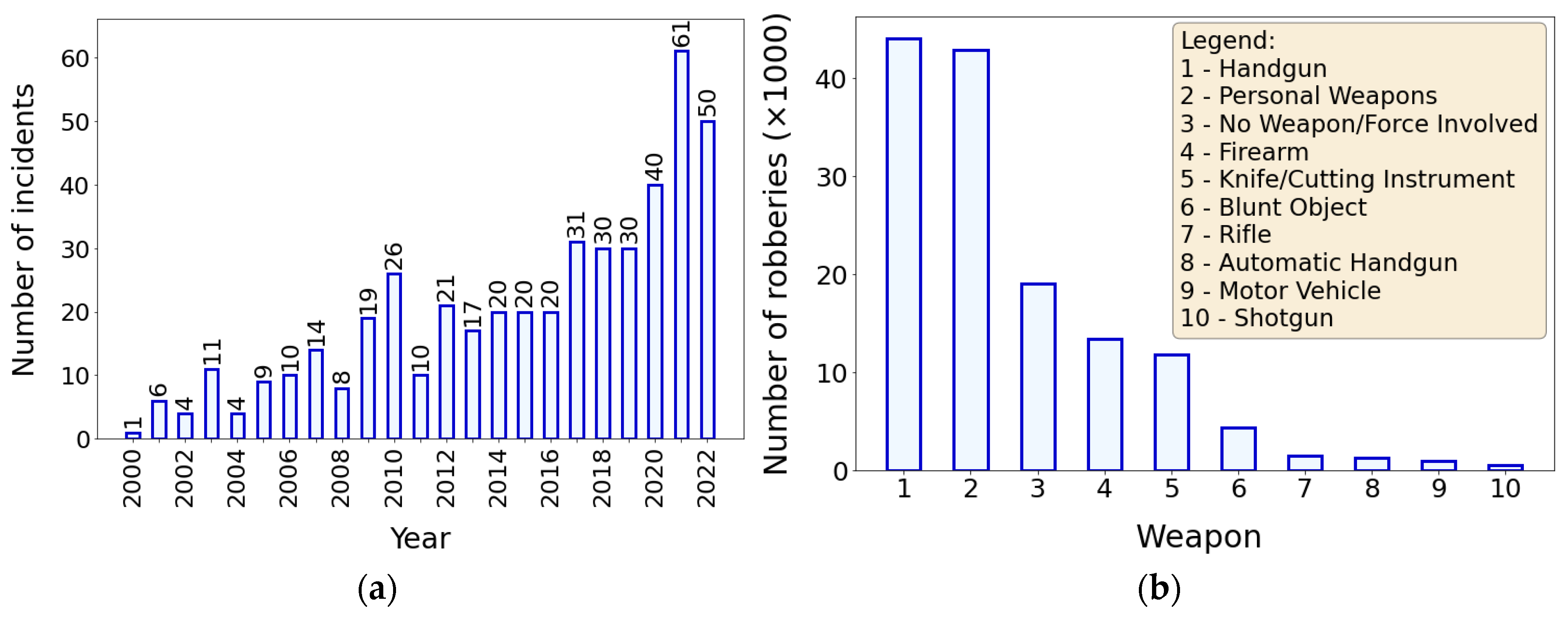
Figure 2.
Number of robberies in the United States in 2022, by location category [2].
Figure 2.
Number of robberies in the United States in 2022, by location category [2].
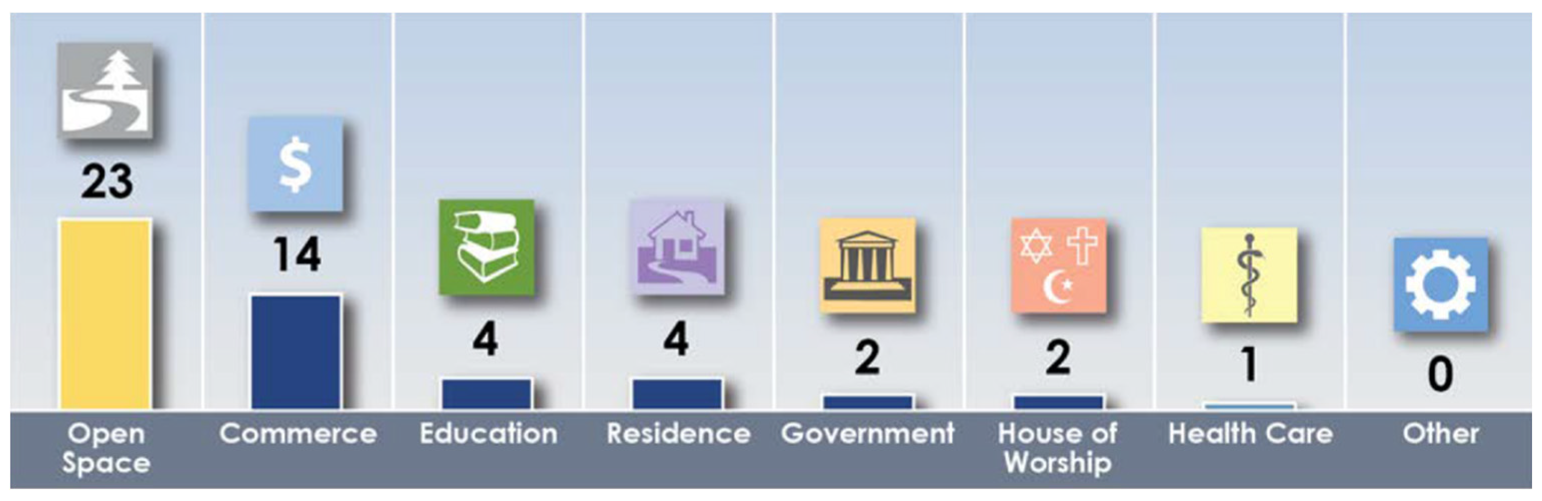
Figure 4.
Illustration of IoU parameter for predicted box Bp (blue) and ground-truth box Bgt (red).
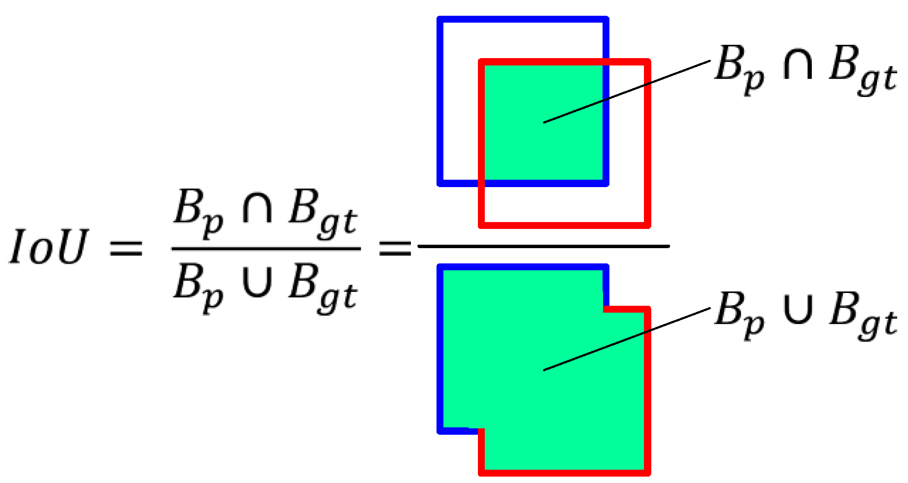
Figure 5.
Example images showing the presentation quality of objects subject to detection: (a) objects clearly visible; (b) objects partially covered; (c) small objects; (d) poor objects sharpness; (e) poor objects illumination.
Figure 5.
Example images showing the presentation quality of objects subject to detection: (a) objects clearly visible; (b) objects partially covered; (c) small objects; (d) poor objects sharpness; (e) poor objects illumination.
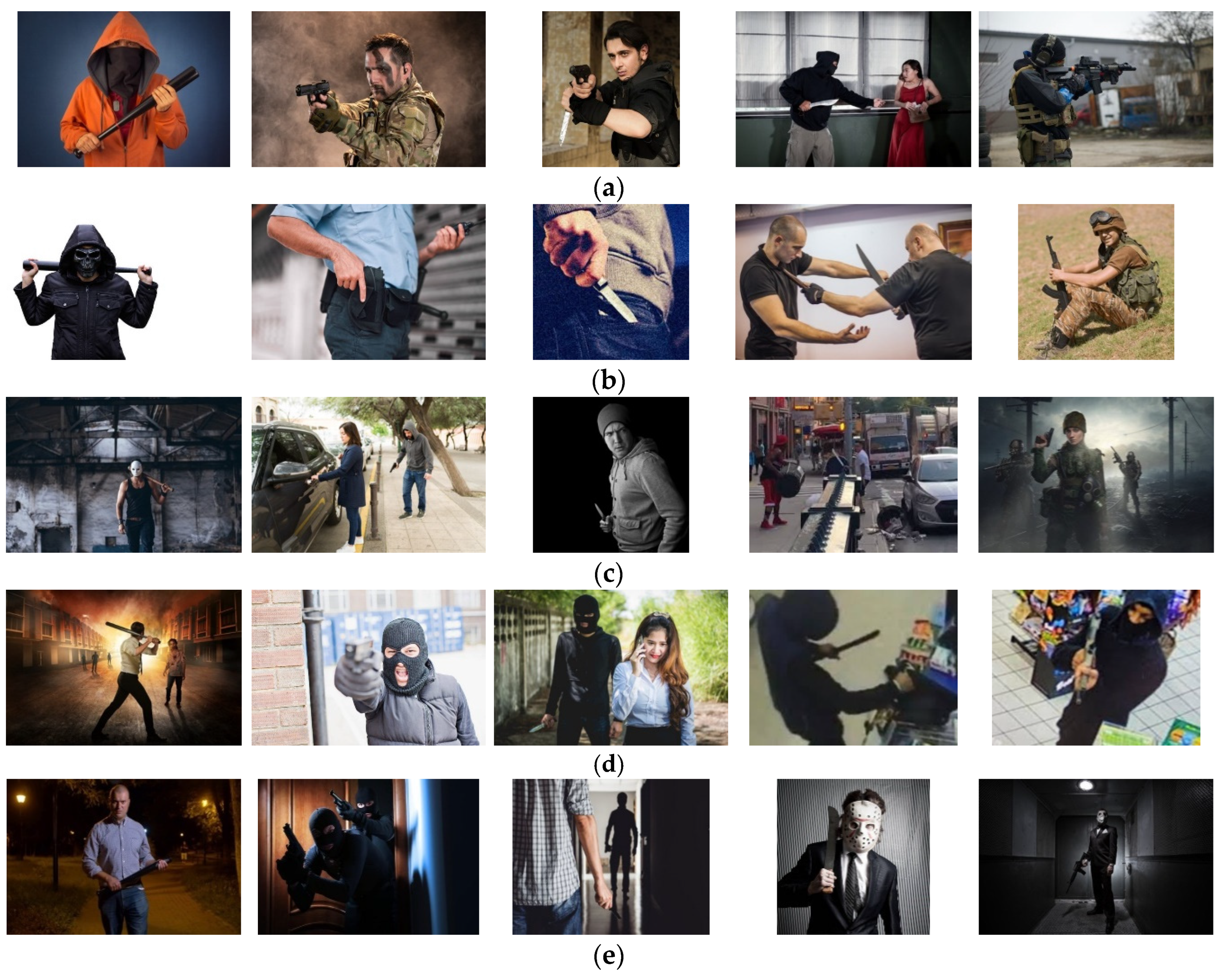
Figure 6.
The number of detected objects in the full (a), training (b) and test (c) datasets.
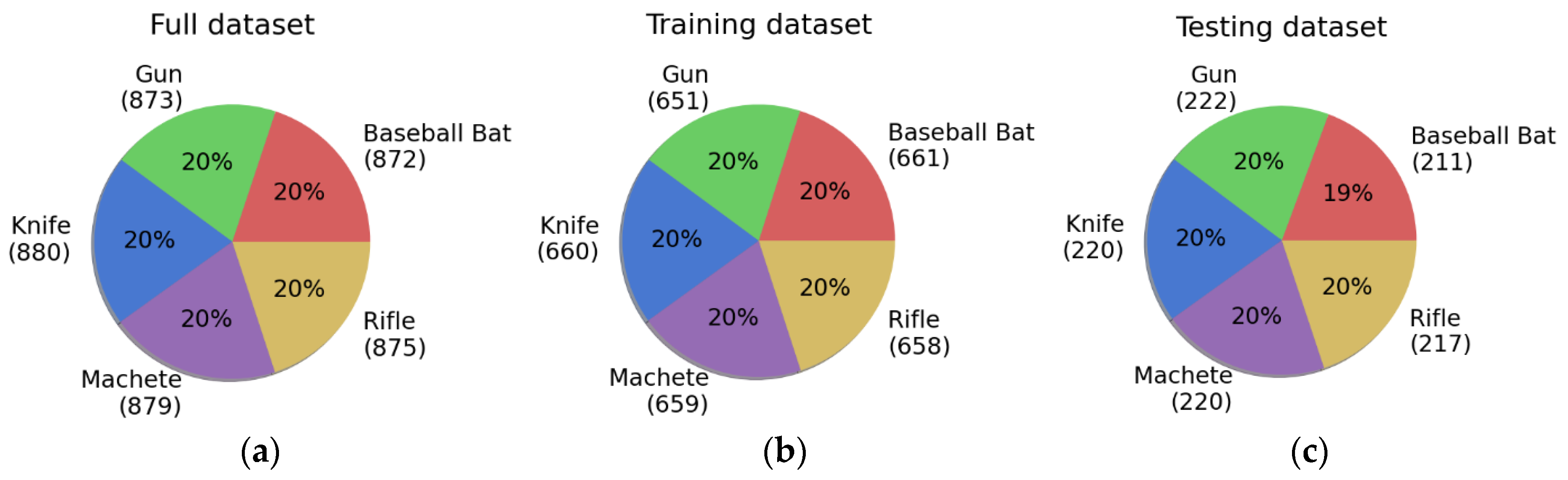
Figure 7.
Network training results: (a) RPN Class Loss; (b) RPN Regression Loss; (c) Detector Class Loss; (d) Detector Regression Loss; (e) Total Loss; (f) Mean Average Precision.
Figure 7.
Network training results: (a) RPN Class Loss; (b) RPN Regression Loss; (c) Detector Class Loss; (d) Detector Regression Loss; (e) Total Loss; (f) Mean Average Precision.
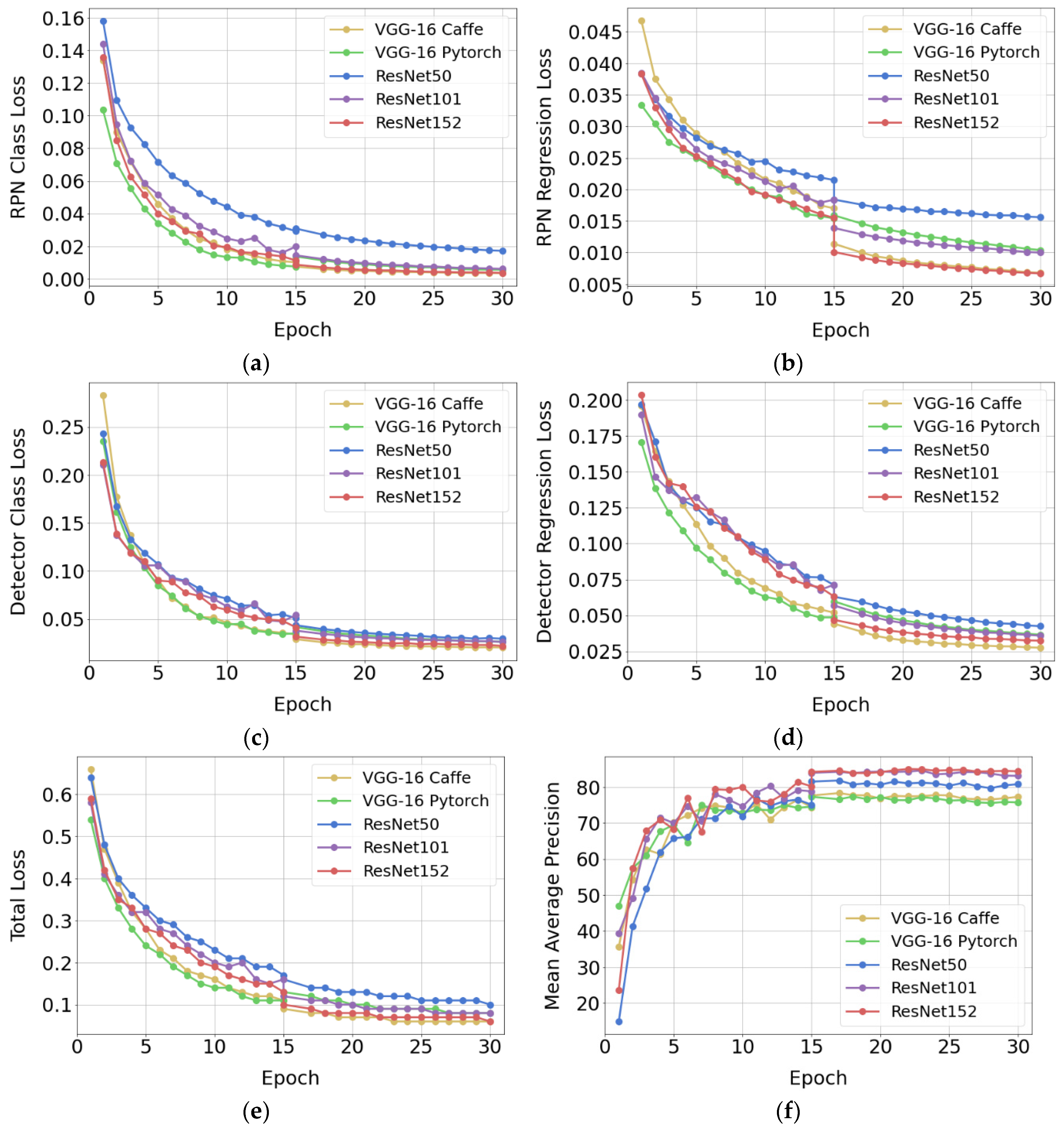
Figure 8.
Precision-recall plots for each category of detected objects: (a) baseball bat; (b) gun; (c) knife; (d) machete; (e) rifle.
Figure 8.
Precision-recall plots for each category of detected objects: (a) baseball bat; (b) gun; (c) knife; (d) machete; (e) rifle.
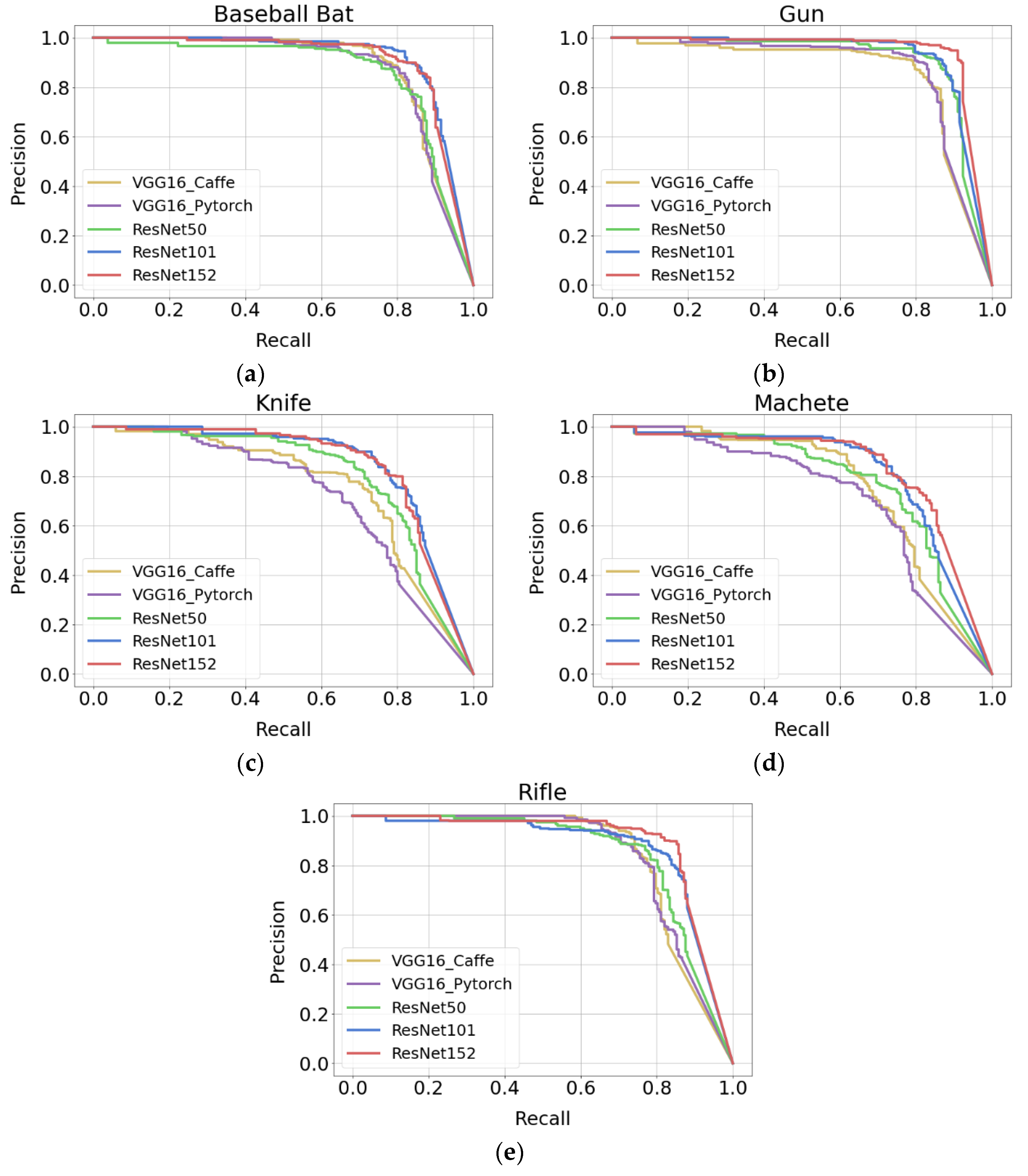
Figure 9.
Average precision of the object detection for individual backbone networks. The average precision was measured for an IoU threshold of 0.5.
Figure 9.
Average precision of the object detection for individual backbone networks. The average precision was measured for an IoU threshold of 0.5.
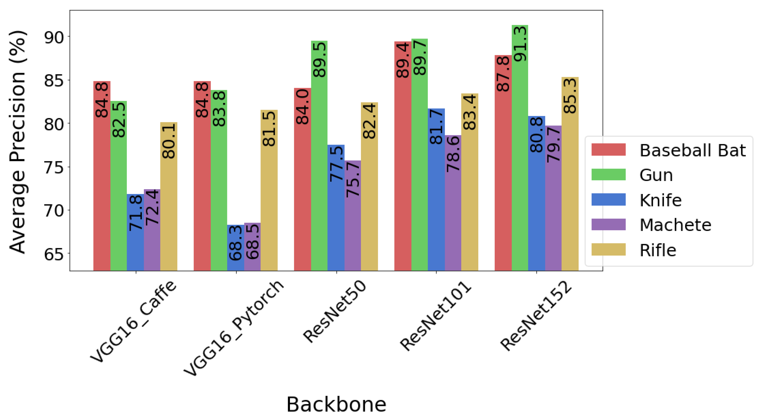
Figure 10.
Mean average precision for individual backbone networks.
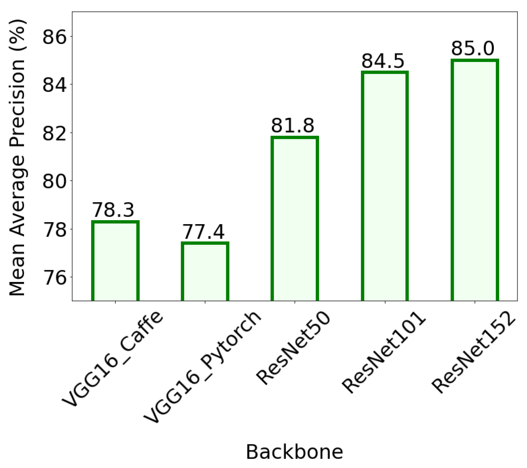
Figure 11.
Inference time averaged over 1000 test images.
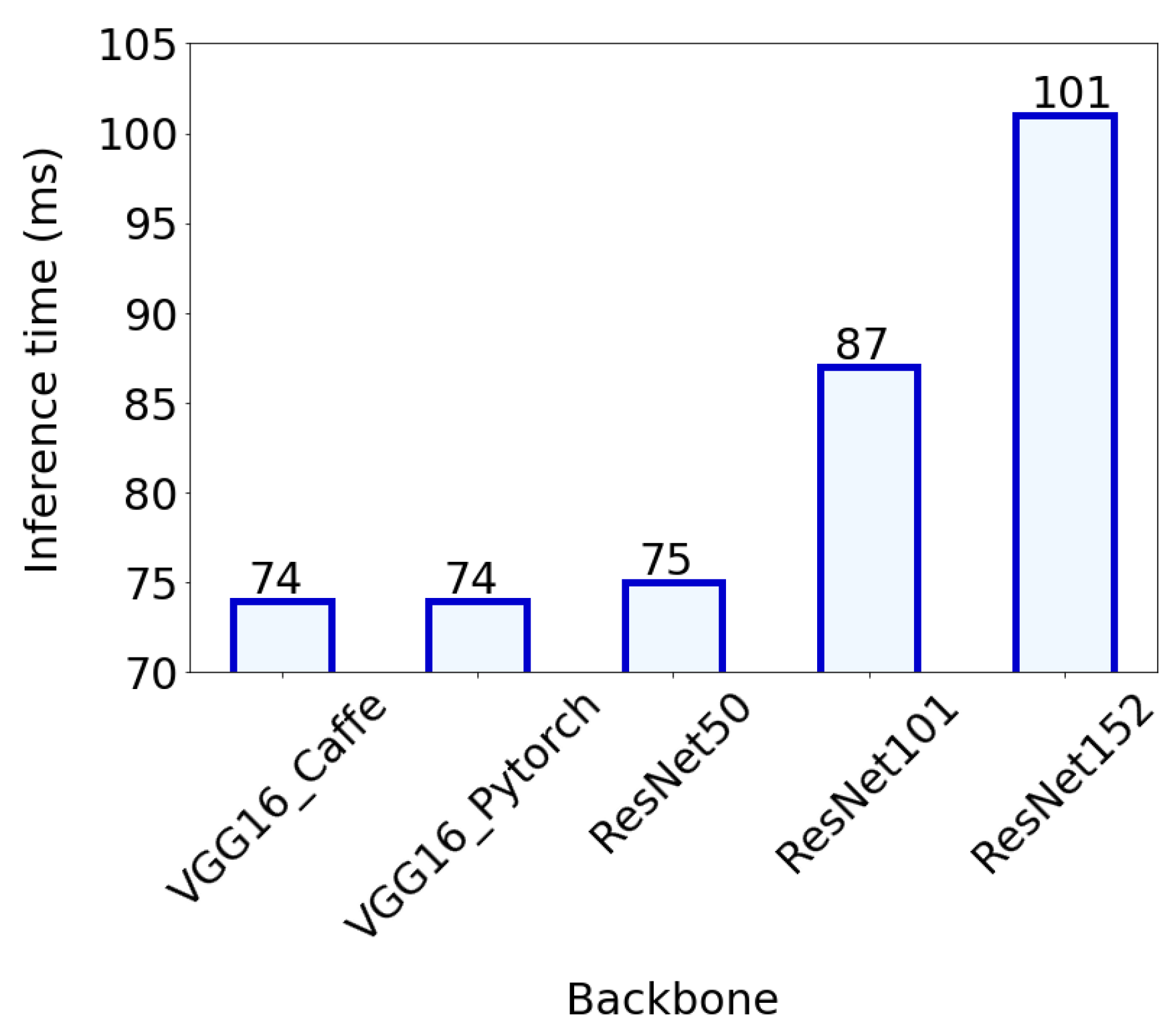
Figure 12.
Example results of detecting objects presented with different quality: (a) objects clearly visible; (b) objects partially covered; (c) small objects; (d) poor objects sharpness; (e) poor objects illumination. Ground-truth bounding boxes are drawn in green and prediction results are marked in red. The images have been cropped so that it is easier to compare the location of ground-truth and predicted bounding boxes.
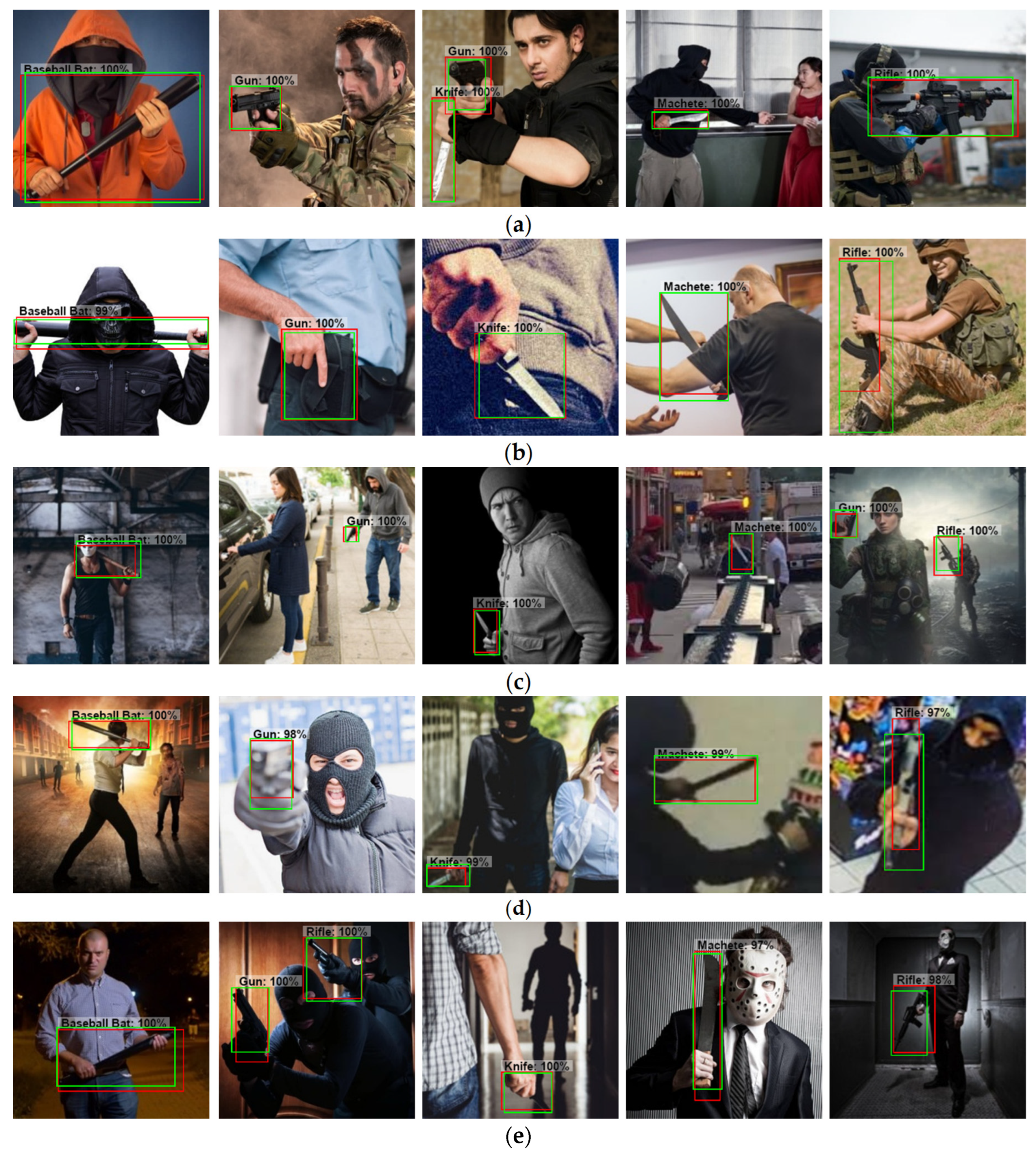
Figure 13.
Evaluation results of the model with the ResNet152 backbone: (a) confusion matrix; (b) recall of the model for individual items.
Figure 13.
Evaluation results of the model with the ResNet152 backbone: (a) confusion matrix; (b) recall of the model for individual items.
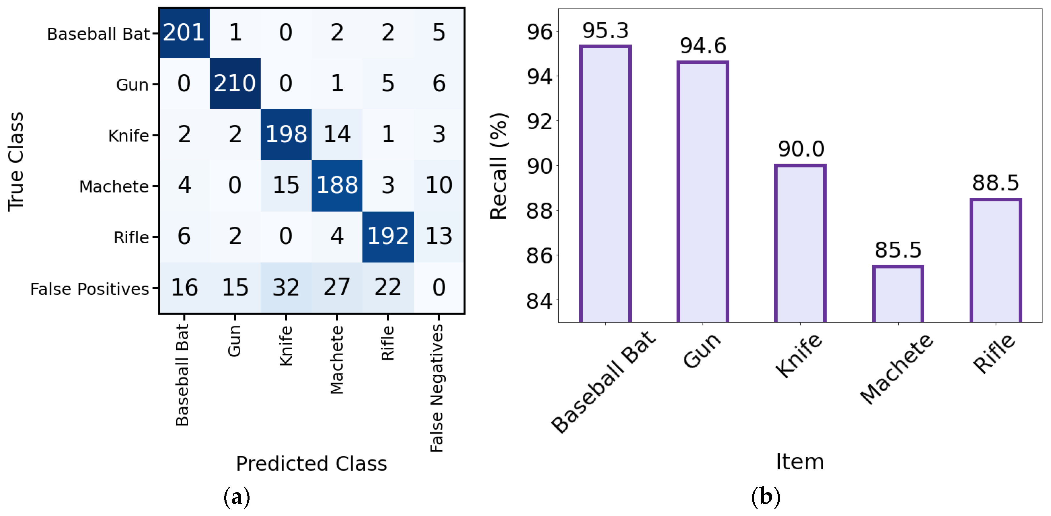
Figure 14.
Selected image frames recorded during detection of dangerous items in people entering the room: (a) objects clearly visible; (b) objects partially covered; (c) small objects; (d) poor objects sharpness; (e) poor objects illumination. For cases (a), (b), (d) and (e) the camera distance and installation height were 2.5 m. For case (c) the camera distance was increased to 5 m. The original image frame size was 800×600 pixels. In order to better present the detected objects, they were cropped to 600×600 pixels.
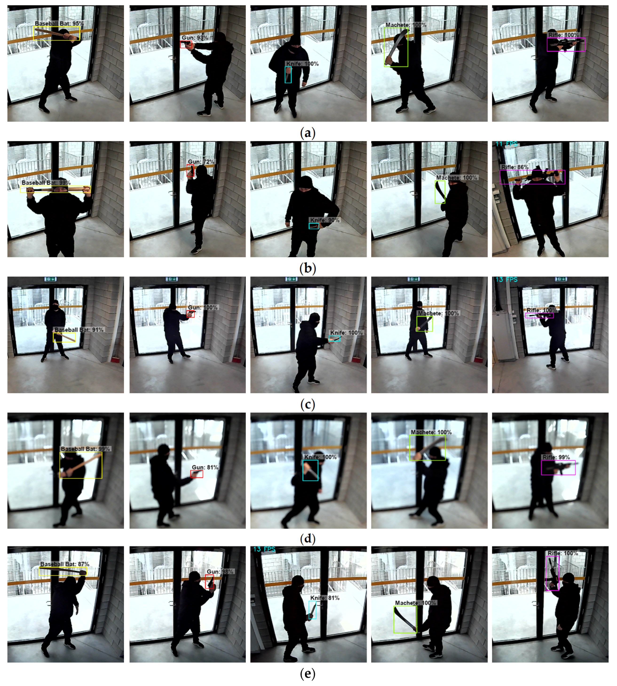

Table 1.
Hyperparameter values used during the models training process.
| Name | Value |
|---|---|
| Epochs | 30 |
| RPN mini-batch | 256 |
| Proposal batch | 128 |
| Object IoU threshold | 0.5 |
| Background IoU threshold | 0.3 |
| Dropout | 0.0 |
| Loss function | multi-task loss function 1 |
| Optimizer | stochastic gradient descent (SGD) |
| Learning rate | 10-3 (epochs 1-15), 10-4 (epochs 16-30) |
| Momentum | 0.9 |
| Weight-decay | 5×10⁻⁴ |
| Epsilon | 10-7 |
| Augmentation | – |
1 multi-task loss function combines classification and regression losses. The meaning of the selected hyperparameters: RPN mini-batch—the number of ground truth anchors sampled for training at each step. Proposal batch—the number of region proposals to sample at each training step. Object IoU threshold—object IoU threshold between an anchor and a ground truth box above which an anchor is labelled as an object (positive) anchor. Background IoU threshold—background IoU threshold below which an anchor is labelled as background (negative).
Table 2.
Total training time.
| VGG-16 Caffe | VGG-16 Pytorch | ResNet50 | ResNet101 | ResNet152 |
|---|---|---|---|---|
| 3h 43m 10s | 4h 10m 39s | 3h 42m 9s | 4h 17m 10s | 6h 25m 13s |
Table 3.
Results of similar studies using Faster R-CNN. A standard IoU threshold of 0.50 was used for all measures.
Table 3.
Results of similar studies using Faster R-CNN. A standard IoU threshold of 0.50 was used for all measures.
| No. in Refs. | Backbone | mAP0.5 (%) | AP0.5 (%) | mAR0.5 (%) | AR0.5 (%) |
|---|---|---|---|---|---|
| Own results | ResNet152 | 85.0 (baseball bat, gun, knife, machete, rifle) |
87.8 (baseball bat) 91.3 (gun) 80.8 (knife) 79.7 (machete) 85.3 (rifle) |
90.6 (baseball bat, gun, knife, machete, rifle) |
95.3 (baseball bat) 94.6 (gun) 90.0 (knife) 85.5 (machete) 88.5 (rifle) |
| [6] | CNN | – | 84.7 (gun) | – | 86.9 (gun) |
| [8] | CNN | 84.6 (gun, rifle) | – | – | – |
| [10] | VGG-16 | – | 84.2 (gun) | – | 100 (gun) |
| [24] | 80.5 (axe, gun, knife, rifle, sword) |
96.6 (gun) 55.8 (knife) 100 (rifle) |
65.8 (axe, gun, knife, rifle, sword) |
61 (gun) 52 (knife) 96 (rifle) |
|
| [25] | VGG-16 | 79.8 (gun, rifle) |
80.2 (gun) 79.4 (rifle) |
– | – |
| [26] | Inception-ResNetV2 | – | 79.3 (gun) | – | 68.6 (gun) |
| [27] | ResNet50 | – | 88.12 (gun) | – | 100 (gun) |
| [28] | Inception-ResNetV2 | – | 86.4 (gun) | – | 89.25 (gun) |
| [29] | SqueezeNet | – | 85.4 (gun) | – | – |
| GoogleNet | – | 46.7 (knife) | – | – |
Disclaimer/Publisher’s Note: The statements, opinions and data contained in all publications are solely those of the individual author(s) and contributor(s) and not of MDPI and/or the editor(s). MDPI and/or the editor(s) disclaim responsibility for any injury to people or property resulting from any ideas, methods, instructions or products referred to in the content. |
© 2024 by the authors. Licensee MDPI, Basel, Switzerland. This article is an open access article distributed under the terms and conditions of the Creative Commons Attribution (CC BY) license (http://creativecommons.org/licenses/by/4.0/).
Copyright: This open access article is published under a Creative Commons CC BY 4.0 license, which permit the free download, distribution, and reuse, provided that the author and preprint are cited in any reuse.


