Submitted:
13 June 2024
Posted:
13 June 2024
You are already at the latest version
Abstract
The capacitated multi-item lot-sizing problem abbreviated as CLSP, is to determine the lot sizes of products in each period in a given planning horizon of finite periods meeting the product demand and resource limits in each period, and minimize the total cost consisting of production, inventory holding, and setup costs. CLSPs are often encountered in industry production settings and thus the solution is significant. In this paper, we propose a Lagrange relaxation (LR) approach for the solution of its. The approach decomposes the CLSP into several uncapacitated single-item lot-sizing problems each of which can be easily solved by dynamic programming. The feasible solutions are achieved by solving the resulting transportation problems with a proposed stepping-stone algorithm and a fix-up procedure. The Lagrange multipliers are updated by using subgradient optimization. Experimental results show that the LR approach explores high-quality solutions and has better applicability compared with other commonly used solution approaches in the literature.
Keywords:
Lagrange relaxation
; lot-sizing
; CLSP
; subgradient optimization
1. Introduction
The capacitated multi-item lot-sizing problem referred to as CLSP is often encountered in industry production settings where multiple products are produced and a bottleneck resource exists [1,2,3]. The problem is to determine the production lot sizes of products and timing over a finite number of periods so that the total cost consisting of production costs, set-up costs, and inventory costs is minimal and meets the production demand of each product in each period. Mathematically, the CLSP can be formulated as follows.
where the meanings of the notations are as follows.
Indices and sets:
i product
t period
I set of products
T set of periods
Parameters:
pit unit linear production cost for the product i in period t
hit unit inventory holding cost for one unit of product i between periods t and t+1
sit setup cost for the product i in period t
dit demand of product i in period t
ai unit capacity requirement for the product i
Ct available capacity in period t
M a large positive number
Variables:
xit amount of product i produced in period t
Iit inventory of product i at the end of period t
yit binary variables, =1, if xit >0; =0, xit =0
In the CLSP, the objective function (1) minimizes the total production, inventory holding and setup costs. Constraint (2) represents the inventory balance, where for any product i the production in period t plus the remaining inventory at the end of period t-1 minus the demand in period t is equal to the inventory at the end of period t. Constraint (3) is the capacity constraint for the bottleneck resource. The capacity consumption of all products in each period t cannot exceed the available amount in that period. Constraint (4) is the associated relation of variables x and y, where a product i is produced in a period t if and only if it has been set up in that period. Constraints (5) - (7) define the decision variables. Note that inventories are non-negative meaning no backlogs allowed. Note also that when production costs do not change over time, the first cost in the objective function is constant and can be removed. The problem often encountered in many important industry application areas, such as production planning and scheduling, logistics management and quality control, etc., is NP-hard [4], thus the solution of the CLSP has continuously been a hot research area in both industry and academic communities [5,6,7].
2. Literature Review
Many publications about the subject of “lot-sizing or lot sizes” can be found in the literature [8,9]. Lot sizing problems can be traced back to the EOQ problem [10], the economic ordering quantity model. EOQ is a trade-off of ordering/setup cost and inventory holding cost to achieve the optimal economic lot sizes. EOQ supposes that the problem is for a single product, stationary, invariable demand, and unlimited production capacity. EOQ can be solved with differential methods. While some complex characteristics are added to the “lot sizes” problem, the problems will be very difficult to solve. For example, when product demand changes over time, more products are produced, etc. However, one of the most essential changes for problem-solving is the existence of production capacity constraints. Consequently, the complexity of a lot-sizing problem can be characterized in terms of the length of the horizon, number of items, and capacity constraints. Based on these characteristics, the lot-sizing problems can be classified into the uncapacitated single-item lot-sizing problem (SILSP), the capacitated single-item lot-sizing problem (CSILSP), the uncapacitated multi-item lot-sizing problem (ULSP), and the capacitated single-level multi-item lot-sizing problem (CLSP). Among them, CLSP is the most common and difficult problem, which has become the core of lot-sizing problem research. However, the SILSP is the simplest lot sizing problem specific to a single product, finite planning horizon of T periods, and no capacity constraints. The SILSPs are solvable in O (T2), except for some variants with some essential extensions, such as setup time and (or) cost, backlogs, time windows, etc., which are NP-hard. The ULSPs are the extension of the SILSPs with multiple items and thus are also solvable in O (T2). The CSILSPs are the extension of the SILSPs with capacity constraints and NP-hard [4]. The CLSP is the extension of CSILSP with multiple items, thus NP-hard. Because of the difficulties of the CLSP, most of the existing solution approaches are heuristic and the exact solution approaches are only for the small-sized problems. In general, the solution approaches to CLSP can be divided into three classes: common heuristics, meta-heuristics, and mathematic programming-based approaches.
Heuristics is sometimes the unique choice when the capacity constraints are very tight in a CLSP. The well-known common heuristics include lot-for-lot, least unit cost (LUC) [11], part-period balancing (PPB) [12,13], Silver-Meal (SM) [14], Lambrecht-Vanderveken (LV) [15], and Dixon-Silver (DS) [16] heuristics. Lot-for-lot heuristic directly converts the demand matrix to a lot-size matrix to obtain an initial solution. This approach maximizes the setup costs and minimizes the inventory holding costs. It is suitable for problems with looser capacity constraints and can quickly obtain an initial feasible solution. LUC heuristic tracks the least cost per unit for production, it can be expressed mathematically as:
Here and after, s indicates the setup cost, h, unit inventory holding cost. The PPB heuristic aims at seeking the maximum production over the demand of several periods when the total holding cost does not exceed a single setup cost. Expressed by the formula:
The SM heuristic attempts to minimize the average cost per unit time for each lot. Mathematically, it can be expressed as:
The LV heuristic is an extended Eisenhut heuristic [17]. LV’s idea is analogous to Eisenhut's heuristic, a period-by-period heuristic. Because we always may suppose that the current period is 1, the LV then computes the maximum order up to the period:
Suppose that, this means that from period 2 to period t*, the cumulative demands exceed the cumulative capacity byunits that must be backward shifted to period 1. Repeat the above process until the current period is T and a feasible solution is obtained. DS heuristic can be regarded as an extension of the SM heuristic for multiple items. Because the single-item SM heuristic for the multiple-item lot-sizing problems is not necessarily optimal even feasible if the capacity limitations exist. Consequently, for a multiple items problem, the DS would be to increase the item which results in the largest decrease in average costs per unit time per unit capacity.
, denotes the average cost per unit time of a lot of item i which will satisfy Ti periods’ requirements. Therefore, ui indicates the marginal decrease in average costs per unit of capacity absorbed under increasing the production of item i from Ti to Ti+1.
Mathematic programming-based approaches are suited for lot-sizing problems with complex constraints and multiple items. The well-known W-W [18] dynamic programming method is for the uncapacitated single-item lot-sizing problem. It solves the USLP in time O (T2). Barany et al. [19] proposed a linear Programming (LP) based approach for CLSP. This approach embeds valid inequalities into a branch and bound framework to solve the linear programming relaxation of the CLSP. Up to 20-item×13-period CLSPs are solved optimally with this approach. Lasdon and Terjung [20] used column generation and generalized upper bound for solving CLSP. Up to 393-item × 6-period CLSPs are solved with their approach with good approximation. Bahl [21] proposed a column generation heuristic for CLSP, where the time-consuming W-W dynamic programming algorithm is replaced by the PPB heuristic in computing shadow prices thus reducing CPU time with a slight loss in optimality. Hindi [22] proposed a variable redefinition approach for the CLSP. The approach uses computationally efficient approaches, such as shortest-path and minimum-cost network flow for obtaining low bounds and upper bounds in a branch and bound framework. Results show the frequent generation of good upper bounds. Thizy and Wassenhove [23] proposed a Lagrangian relaxation approach for CLSP. The Lagrangian relaxation problem consists of |I| uncapacitated single-item problems and each of them is solved with the W-W dynamic programming in O (T2). Feasible solutions are obtained from the resulting transportation problems with specified production periods. The Lagrange multipliers are updated by a subgradient procedure [24]. Trigeiro et al. [25] proposed a Lagrangian relaxation for CLSP with setup times. They relax the capacity constraints to the objective function and solve these decomposed single-item problems with the W-W dynamic programming. Finding feasible solutions is by a heuristic called smooth procedure. Diaby et al. [26] proposed a Lagrangian relaxation for CLSP in which Lagrangian relaxation is used within a framework of branch and bound algorithm to generate bounds. Initial upper bounds are generated by three heuristics: (1) DS heuristic (2) a linear programming-based relaxation and (3) an extension of the solution procedure of Thizy and Van Wassenhove [23] with setup times and multiple resources. Practical-sized problems are tested and the results are very well.
Meta-heuristics have also been used to solve CLSP for many applications. Xie and Dong [27] proposed a heuristic genetic algorithm (GA) for CLSP. They design a domain-specific encoding scheme for lot sizes and provide a heuristic shifting procedure for decoding. Computational results show that the algorithm converges a solution within 200 generations for most of the small-scale examples (N ≤10) and within 500 generations for most of the modest examples (N ≤20). Gaafar [28] applied a genetic algorithm (GA) to solve dynamic lot-sizing with batch ordering and backorders. The approach uses a “012” coding scheme specific to the problem. Computational results show that the proposed genetic algorithm outperforms the modified SM heuristic in terms of optimal rate and percentage deviation. Gaafar et al. [29] proposed a simulated annealing (SA) algorithm for lot-sizing problems. In their algorithm, the “012” coding scheme and 16 mutation-based moves are used for solving dynamic lot-sizing problems and the computational results show the performance of the SA outperforms the compared GA and the modified SM heuristic. Hindi [30] proposed a tabu search (TS) heuristic for CLSP. In his implementation, firstly, a reformulation of the original problem is executed by variable redefinition. The new problem has tighter bounds but more variables and thus is solved by column generation. The resulting feasible solution is further improved by solving a minimum-cost network flow problem, and then the improved solution is used as a starting point for a tabu search procedure. Computational results show the effectiveness of the TS. More solutions for CLSP with metaheuristics are referred to [31].
In this paper, we propose a Lagrange relaxation approach for the CLSP, the work is closely related to that of [23]. However, the difference is clear in the methods for finding the low bounds and upper bounds. The contributions of this paper are as follows.
- (1)
- A Lagrange relaxation approach for CLSP is implemented.
- (2)
- A stepping-stone algorithm is developed for solving the resulting transportation problem.
- (3)
- A fix-up heuristic is proposed for obtaining feasible solutions.
- (4)
- A local neighborhood search heuristic is used for further searching for high-quality solutions, which increases the chance of finding the optimal solution.
3. Solution Approach
3.1. Lagrange Relaxation
We propose a Lagrange relaxation approach for CLSP [32,33]. Let ut, t =1, ..., T, be nonnegative Lagrange multipliers for capacity constraints (3), and then a Lagrange relaxation problem (LR (u)) is obtained as follows.
The LR (u) problem can be then decomposed into |I| independent uncapacitated single-item lot-sizing problems, each of which is solvable in O(T2) [18], any of the previously mentioned single-item problem methods, for example, lot-for-lot, LUC, W-W dynamic programming, etc., can be used for this aim. In this paper, the W-W dynamic programming is chosen. Note that for any given u, the solution of the LR(u) will give a lower bound zLB for the original problem (CLSP).
3.2. Obtaining Feasible Solutions
Let (yu, xu, Iu) be the optimal solution of zu for a given u, note that when the production periods are specified by fixing yit at 0 or 1 for all i = 1, …, I, t = 1, …, T, the problem can be transformed into a transportation problem with |T| origins and |T|×|I| destinations. Also, note that some of the arcs of the transportation problem are forbidden due to both preventing backlogging or production not starting in that period.
The transportation problem (TP) is formulated as follows.
s.t.
: the amount of product i produced in the period t help satisfy the demand in the future period.
To solve the resulting transportation problem TP (y), we developed a stepping-stone algorithm [34,35]. The algorithm is shown in Algorithm 1.
| Algorithm 1: Stepping-stone algorithm |
|
Note that the solution to the transportation problem will give an upper bound zUB of the CLSP if it is feasible. As an illustrative example from the literature [23], here, a 3-item×4-period CLSP with specified y is considered. The problem and data are shown in Table 1, Table 2 and Table 3. The iteration process of the algorithm is shown in Table 4, Table 5, Table 6, Table 7 and Table 8.
In Table 1, a number with a square indicates that the production in the period occurs. In Table 3, the resulting transportation problem is formed with y specified in Table 1. The marks X and X indicate the corresponding arcs are forbidden either because yit = 0 or because, respectively. The initial basis is listed in Table 4. The superscripts are the basis variable labels. The initial objective value is 385.3(no setups included). The optimal solution is obtained with 4 iterations and the objective values are gradually reduced to 285.3, 193.3, 162.3, and 146 (optimal). The four closed-loops found are (14-1-0), (10-12-13-1-0-14-15), (13-1-0-14-15-10-4), and (13-1-0), marked with purple dotted boxes.
3.3. Fix-up Heuristic
For a given yu, from the LR(u), the resulting transportation problem TP(y) often is infeasible. To obtain a feasible solution, we introduce a fix-up policy to make it feasible. The fix-up policy shifts lots among periods using lot techniques. The fix-up heuristic is shown in Algorithm 2.
| Algorithm 2: Fix-up heuristic |
|
Check infeasible period cp, compute the remaining capacity RCj,
, for each period j=1,…,T.
If (cp < T) go to forward pass; else go to backward pass.
Forward pass: for each product check inventory period by period, forward move products lots into periods cp+1, cp+2,…, T, with a cost-effective fashion until no sufficient capacity is available. Go to 4
Backward pass: if the following periods no excessive capacities exist, backward move products lots into periods cp-1, cp-2,…, with cost-effective fashions.
Iteratively execute 3 and 4, until a feasible solution is obtained.
3.4. Local Neighborhood Search Algorithm
to find more high-quality solutions, we proposed a local neighborhood search algorithm for the current feasible solution. The neighborhood structures are defined as follows.
- (1)
- The neighborhood of the lot-move
The first neighborhood structure is for shifting lots between two periods for a single item. Assume there exists an item i, and any two periods t1 and t2, two lots> 0,> 0, in that corresponding periods, and again assume there are no positive lots among t1 and t2. The neighborhood of lot-move is then defined for all possible moves between t1 and t2 as above stated. As an illustrative example, let> 0 be the lot from period t1 to period t2, then have
Note that the lot move may be bidirectional. The forward move reduces inventories, while the backward move may reduce setups. The cost change can be computed from formula (15), (16).
When the inventory cost hi changes from period to period, the formula needs to adjust correspondingly. The cardinal of the lot-move neighborhood is O(n3).
- (2)
- The neighborhood of the 2-opt lot-exchanges
The neighborhood is for the 2-opt lot-exchanges which change lots for two items in two continuous periods. Assume there are two items i1, i2, and two continuous periods, t1 and t2, the related lots are, respectively. Now we swap two lots for two items i1 and i2 and two continuous periods t1 and t2, and assume that,, then have , for forward exchange,, for backward exchange.
The cardinal of the neighborhood is O(n4).
As an illustrative example, below a 3-item×4-period lot-sizing problem is considered [15]. The data is referred to in the literature. The 2-opt lot-exchange local neighborhood search results are shown in Figure 1.
The initial solution is obtained from the DS heuristic, and the objective function is 1415.7. Two 2-opt lot exchanges were performed and two improved solutions were obtained with values of 1414 and 1412.6, optimal.
3.5. Subgradient Algorithm
For a given u, the solution of the TP(y) gives an upper bound of the original problem. To obtain the maximum upper bound, the traditional subgradient algorithm [31] is selected in this paper. By subgradient theories, is a subgradient of function zu at point u. The Lagrange multipliers u are updated using the formula.
where, is the solution of LR (uk), zbest is the best upper bound found, η0= 2. The subgradient algorithm is shown in Algorithm 3.
| Algorithm 3: Subgradient algorithm |
| 1: given a Lagrangian multiplier uk, k = 0; 2: loop 3: Arbitrarily select a subgradient from ∂(zu), If any of the termination criteria are met then stop; else uk+1 = max {0, uk + θksk}; 4: k=k+1; 5: if k > N then stop; 6: end loop |
Notes: 1. selection of θk:
;
- θk = θ0ρk, 0<ρ<1;
- ;
- 3
- Iterations: N,
- 4
- sk = 0 or,
- 5
- |zUBk - zLBk| < ε
- 6
- uk or z(uk) does not change within a given number of iterations (e.g., 7).
3.6. Overview of the Lagrange Relaxation Algorithm
Based on the description of the components of the algorithm, we give the complete algorithm framework as shown in Algorithm 4.
| Algorithm 4: Lagrangian relaxation main procedure |
| // Initialization 1: k =0 2: LB = -1E+10 // a sufficiently small lower bound 3: UB = 1E+10 // a sufficiently large upper bound 4: Gap = 1E-2 // dual gap percentage 5: K = 5000 // the maximum number of iterations 6: ηk = 2.0 // step-size 7: uk = 0 // Lagrangian multipliers 8: loop // main cycle beginning 9: Solve the Lagrangian relaxation LR (uk) by the W-W dynamic programming, and calculate the current lower bound ZLB (uk) 10: Solve the resulting transportation problem by the stepping-stone algorithm for the y from the solution of the current LR to obtain a ZUB (uk) if it is feasible else { Execute fix-up heuristic Solve the corresponding transportation problem using the stepping-stone algorithm } 11: Execute the local neighborhood search algorithm for raising solution quality 12: if ZLB (uk) < ZLB, ZLB = ZLB (uk) // update low bounds 13: if ZUB (uk) >ZUB, ZUB = ZUB (uk) // update upper bounds 14: if [ (ZUBk – ZLBk) / ZUBk] ≤ Gap, then stop 15: k++, if k >= K then stop; 16: Update Lagrangian multipliers with the subgradient algorithm 17: ηk =1/2*ηk; // update step-size 18: end loop // main cycle ending |
4. Computational Results
4.1. Comparison Study
The solution approach proposed in this paper has been implemented on a personal computer using VC++ 6.0 programming language. Computational experiments for the benchmarks and the randomly generated large-sized CLSPs are performed. The benchmarks are from the literature [23]. The computational results are listed in Table 10. The data is listed in Table 9.
The computational results are listed in Table 10. Four approaches, LRFN (the proposed approach), LR (without the local neighborhood search), DS, and LV are compared, wherein the results of DS and LV are from the literature [23], and the optimal solutions are from CPLEX 7.0. We can see that the LRFN proposed in this paper is better than others. For the problems with looser capacity, where the capacity utilization ratios are below 73% of TVW3 and TVW4, the LRFN obtains the optimal solution. For the problems with tighter capacity, TVW2, where the capacity utilization ratio is 91%, LRFN obtains the optimal solution, others obtain the near-optimal solutions, especially, and LV has a larger error, about 11.3%. For the tightest capacity problem, TVW1, where the capacity utilization ratio is 93%, LRFN obtains the best near optimum, and the error is below 1%, but the errors of DS and LV are 3.3% and 6.4%, respectively.
4.2. Large-Sized Problems
The benchmarks we previously computed had been regarded as large problems in that time (1980s). However, today computer ability has made essential progress. In addition, the difficulty of lot-sizing problems can be evaluated with the following criteria:
- (1)
- The number of time periods, |T| and the number of items, |I|.
- (2)
- Tightness of the capacity utilization: .
Thus, we compute the larger problems at different difficulty levels. The data of these problems are randomly generated and adhere to the following agreements.
- (1)
- the maximal number of items is set to 512;
- (2)
- the number of periods is set to 48;
- (3)
- the maximal utilization ratio is set to 93%.
The other problem-specific data are properly randomly generated, for example, Ct: rand (800, 2000), dit: rand (0,100), si: rand (100, 2000), pi:(1,8), hi:(1,4), and ai=1, and so on. Computational results for these problems are listed in Table 11.
In Table 11, the column “Iteration found” represents that the best solution is found in a certain iteration. The meanings of other columns are clear. As shown in Table 11, the average dual gap is within 2% (exactly 1.76) except for some extreme examples, like problem No. 15 the dual gap is 9.54. The reason for that result may be the excessively tight capacity utilization. Usually, the looser the capacity utilization ratio, the smaller the dual gap is; and vice versa.
5. Conclusions
In this paper, we propose a Lagrange relaxation approach for solving the capacitated multi-item lot-sizing problem, called CLSP. The CLSP is often encountered in industry production settings and studying its solution approaches is significant. Our work mainly includes: (1) developing a stepping-stone algorithm for solving the resulting transportation problem to obtain upper bounds, (2) developing a fix-up procedure for obtaining feasible solutions, (3) developing a local search heuristic for obtaining high-quality solutions. Computational experiments from the benchmarks and the randomly generated large-sized examples verify the effectiveness and efficiency of the proposed solution approach.
Conflicts of Interest:
The author declares no conflict of interest.
Author Contributions
Conceptualization, Z.G. and D.L.; data curation, D.L.; formal analysis, D.W.; methodology, Z.G.; experimental design and testing, D.L.; software, D.W. and Z.Y.; supervision, Z.G.; validation, Z.Y.; writing— original draft, Z.G.; writing—review and editing, D.W.; All authors have read and agreed to the published version of the manuscript.
Funding
This study was partly supported by the Major Program of the National Natural Science Foundation of China (72192830, 72192831), and the 111 Project (B16009).
Data Availability Statement
Data are contained within the article.
References
- Drexl, A.; Kimms, A. Lot sizing and scheduling — Survey and extensions. Eur. J. Oper. Res. 1997, 99, 221–235. [Google Scholar] [CrossRef]
- Maes, J.; Van Wassenhove, L.N. Multi-item single-level capacitated dynamic lot-sizing heuristics: a general review. Journal of the Operational Research Society 1988, 39, 991–1004. [Google Scholar] [CrossRef]
- Karimi, B.; Ghomi, S.F.; Wilson, J. The capacitated lot sizing problem: a review of models and algorithms. Omega 2003, 31, 365–378. [Google Scholar] [CrossRef]
- Florian, M.; Lenstra, J.K.; Rinnooy Kan, A.H. G Deterministic production planning algorithms and complexity. Management Science 1980, 26, 669–679. [Google Scholar] [CrossRef]
- Tang, L.; Meng, Y.; Liu, J. An improved Lagrangean relaxation algorithm for the dynamic batching decision problem: Lot sizing and scheduling: new models and solution approaches to address industrial extensions. International Journal of Production Research 2011, 49, 2501–2517. [Google Scholar] [CrossRef]
- Gao, Z.; Tang, L.; Jin, H.; Xu, N. An Optimization Model for the Production Planning of Overall Refinery. Chin. J. Chem. Eng. 2008, 16, 67–70. [Google Scholar] [CrossRef]
- Zhang, X.; Liu, R.; Ren, J.; Gui, Q. Adaptive Fractional Image Enhancement Algorithm Based on Rough Set and Particle Swarm Optimization. Fractal Fract. 2022, 6, 100. [Google Scholar] [CrossRef]
- Jans, R.; Degraeve, Z. Modeling industrial lot sizing problems: a review. Int. J. Prod. Res. 2008, 46, 1619–1643. [Google Scholar] [CrossRef]
- Buschkühl, L.; Sahling, F.; Helber, S.; Tempelmeier, H. Dynamic capacitated lot-sizing problems: a classification and review of solution approaches. OR Spectr. 2008, 32, 231–261. [Google Scholar] [CrossRef]
- Harris, F.W. How many parts to make at once, Factory – The Magazine of Management, 1913, 10, 135–136+152.
- Gorham, T. Dynamic order quantities. Prod. Inventory Manag. J. 1968, 9, 75–79. [Google Scholar]
- DeMatteis, J.J. An economic lot-sizing technique, I: The part-period algorithm. IBM Syst. J. 1968, 7, 30–38. [Google Scholar] [CrossRef]
- Mendoza, A.G. An economic lot-sizing technique. II: Mathematical analysis of the part period algorithm. IBM Systems Journal 1968, 739–746. [Google Scholar] [CrossRef]
- Silver, E.A.; Meal, H.C. A heuristic for selecting lot size quantities for the case of a deterministic time varying demand rate and discrete opportunities for replenishment. Production and Inventory Management 1973, 14, 64–74. [Google Scholar]
- Lambrecht, M.R.; Vanderveken, H. Heuristics procedures for the single operation, multi-item loading problem, AIIE Transactions 1979, 11, 319–326.
- Dixon, P.S.; Silver, E.A. A heuristics solution procedure for multi-item, single-level, limited capacity, lot-sizing problem, Journal of Operations Management 1981, 2, 23–39.
- Eisenhut, P.S. A Dynamic Lot Sizing Algorithm with Capacity Constraints. A I I E Trans. 1975, 7, 170–176. [Google Scholar] [CrossRef]
- Wagner, H.M.; Whitin, T.M. Dynamic Version of the Economic Lot Size Model. Manag. Sci. 1958, 5, 89–96. [Google Scholar] [CrossRef]
- Barany, I.; Van Roy, T.J.; Wolsey, L.A. Strong Formulations for Multi-Item Capacitated Lot Sizing. Manag. Sci. 1984, 30, 1255–1261. [Google Scholar] [CrossRef]
- Lasdon, L.S.; Terjung, R.C. An Efficient Algorithm for Multi-Item Scheduling. Oper. Res. 1971, 19, 946–969. [Google Scholar] [CrossRef]
- Bahl, H.C. Column Generation Based Heuristic Algorithm for Multi-Item Scheduling. IIE Trans. 1983, 15, 136–141. [Google Scholar] [CrossRef]
- Hindi, K. Computationally efficient solution of the multi-item, capacitated lot-sizing problem. Comput. Ind. Eng. 1995, 28, 709–719. [Google Scholar] [CrossRef]
- Thizy, J.M.; Van Wassenhove, L.N. Lagrangian relaxation for the multi-item capacitated lot-sizing problem, a heuristics approach. AIIE Transactions 1985, 17, 308–313. [Google Scholar]
- Held, M.; Wolfe, P.; Crowder, H.P. Validation of subgradient optimization. Math. Program. 1974, 6, 62–88. [Google Scholar] [CrossRef]
- Trigeiro, W.W.; Thomas, L.J.; McClain, J.O. Capacitated Lot Sizing with Setup Times. Manag. Sci. 1989, 35, 353–366. [Google Scholar] [CrossRef]
- Diaby, M.; Bahl, Karwan, H. M.; Zionts, S. Capacitated lot-sizing and scheduling by Lagrangean relaxation. European Journal of Operational Research 1992, 59, 444–458. [Google Scholar] [CrossRef]
- Xie, J.; Dong, J. Heuristic genetic algorithms for general capacitated lot-sizing problems. Comput. Math. Appl. 2002, 44, 263–276. [Google Scholar] [CrossRef]
- Gaafar, L. Applying genetic algorithms to dynamic lot sizing with batch ordering. Comput. Ind. Eng. 2006, 51, 433–444. [Google Scholar] [CrossRef]
- Gaafar, L.K.; Nassef, A.O.; Aly, A.I. Fixed-quantity dynamic lot sizing using simulated annealing. Int. J. Adv. Manuf. Technol. 2008, 41, 122–131. [Google Scholar] [CrossRef]
- Hindi, K.S. Solving the CLSP by a tabu search heuristic, Journal of the Operational Research Society 1996, 47, 151–161.
- Jans, R.; Degraeve, Z. Meta-heuristics for dynamic lot sizing: A review and comparison of solution approaches. Eur. J. Oper. Res. 2007, 177, 1855–1875. [Google Scholar] [CrossRef]
- Fisher, M.L. The Lagrangian Relaxation Method for Solving Integer Programming Problems. Manag. Sci. 1981, 27, 1–18. [Google Scholar] [CrossRef]
- Fisher, M.L. An Applications Oriented Guide to Lagrangian Relaxation. INFORMS J. Appl. Anal. 1985, 15, 10–21. [Google Scholar] [CrossRef]
- Charnes, A.; Cooper, W.W. The Stepping Stone Method of Explaining Linear Programming Calculations in Transportation Problems. Manag. Sci. 1954, 1, 49–69. [Google Scholar] [CrossRef]
- Glover, F.; Klingman, D. Letter to the Editor—Locating Stepping-Stone Paths in Distribution Problems Via the Predecessor Index Method. Transp. Sci. 1970, 4, 220–225. [Google Scholar] [CrossRef]
Figure 1.
2-opt lot-exchanges for solution improvement.
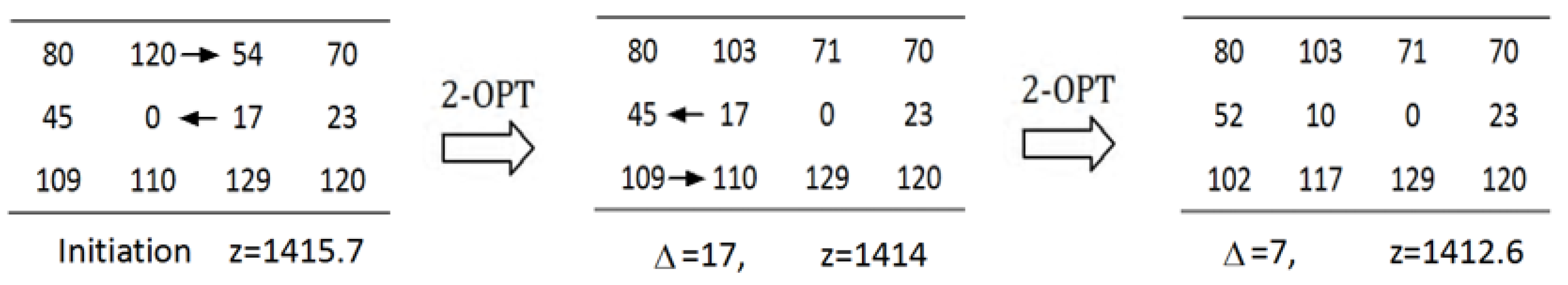

Table 1.
Demand and capacity.
| Item | period | ||||
| 1 | 2 | 3 | 4 | ||
| 1 | 20 | 30 | 40 | 10 | demands |
| 2 | 20 | 10 | 10 | 10 | |
| 3 | 25 | 30 | 30 | 30 | |
| capacity | 450 | 400 | 450 | 300 | |
Table 2.
Other data.
| Item | pi | ai | si | hi |
| 1 | - | 5 | 70 | 3 |
| 2 | - | 4 | 90 | 4 |
| 3 | - | 6 | 200 | 5 |
Table 3.
The transportation problem.
| production | demands | |T|t | ||||||||||||
| 100 | 150 | 200 | 50 | 80 | 40 | 40 | 40 | 150 | 180 | 180 | 180 | 210 | ||
| 450 | 0 | .6 | 1.2 | 1.8 | 0 | 1 | 2 | 3 | 0 | 5/6 | 5/3 | 2.5 | 0 | 1 |
| 400 | X | 0 | .6 | 1.2 | X | X | X | X | X | 0 | 5/6 | 5/3 | 0 | 2 |
| 450 | X | X | 0 | .6 | X | X | 0 | 1 | X | X | 0 | 5/6 | 0 | 3 |
| 300 | X | X | X | X | X | X | X | X | X | X | X | 0 | 0 | 4 |
| |T|×|I|+1 | τ=1,2,3,4; i=1 | τ=1,2,3,4; i=2 | τ=1,2,3,4; i=3 | dummy | ||||||||||
Table 4.
The initial basic feasible solution and 1st closed-loop.
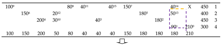 |
Table 5.
The 2nd basic feasible solution and closed-loop.
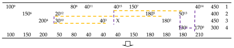 |
Table 6.
The 3rd basic feasible solution and closed-loop.
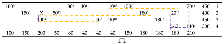 |
Table 7.
The 4th basic feasible solution and closed-loop.
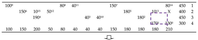 |
Table 8.
The optimal basic solution.
| 1009 | 808 | 4011 | 1507 | 8014 | 450 | 1 | ||||||||
| 1506 | 1015 | 5012 | 1805 | 1013 | 400 | 2 | ||||||||
| 1904 | 403 | 4010 | 1802 | 450 | 3 | |||||||||
| 1801 | 1200 | 300 | 4 | |||||||||||
| 100 | 150 | 200 | 50 | 80 | 40 | 40 | 40 | 150 | 180 | 180 | 180 | 210 |
Table 9.
Data for problems TVW1-4.
| item | hi | si | period | TBO | |||||||
| 1 | 2 | 3 | 4 | 5 | 6 | 7 | 8 | ||||
| 1 | 1 | 100 | - | 70 | 50 | 100 | 20 | 80 | - | 100 | 2 |
| 2 | 1 | 200 | 20 | 40 | 50 | 10 | 30 | - | 40 | 50 | 3.65 |
| 3 | 1 | 200 | 40 | 50 | - | 100 | 40 | 80 | 90 | 160 | 2.33 |
| 4 | 1 | 300 | - | 100 | 100 | 150 | 160 | 90 | 100 | 100 | 2.5 |
| 5 | 1 | 400 | 50 | - | 20 | 40 | 10 | 10 | 20 | 10 | 6.32 |
| 6 | 1 | 250 | 70 | 40 | 40 | 40 | 100 | 20 | 40 | 50 | 3.16 |
| 7 | 1 | 500 | - | 20 | 50 | 10 | 20 | 60 | 40 | 40 | 5.77 |
| 8 | 1 | 300 | 10 | 20 | - | - | 10 | 10 | 20 | 30 | 6.93 |
| Available demand | 190 | 340 | 310 | 450 | 390 | 350 | 350 | 540 | Total demand 2920 |
||
| TVW1 | 350 | 350 | 350 | 400 | 400 | 400 | 400 | 500 | 3150 (93%) | ||
| TVW2 | 400 | 400 | 400 | 400 | 400 | 400 | 400 | 400 | 3200 (91%) | ||
| TVW3 | 500 | 500 | 500 | 500 | 500 | 500 | 500 | 500 | 4000 (73%) | ||
| TVW4 | 600 | 600 | 600 | 600 | 600 | 600 | 600 | 600 | 4800 (61%) | ||
Table 10.
Computational results for benchmarks.
| Problem ID | LP Relaxation | Optimal solution With CPLEX |
LR | LRFN | DS | LV |
| TVW1 | 7996.67 | 8430 | 8710 | 8520 | 8710 | 8970 |
| TVW2 | 7722.27 | 7910 | 7930 | 7910 | 7930 | 8800 |
| TVW3 | 7534.17 | 7610 | 7610 | 7610 | 7970 | 7970 |
| TVW4 | 7446.17 | 7520 | 7520 | 7520 | 8000 | 8000 |
Table 11.
Computational results of the large-sized problems.
| Problem No. |
Problem size (items × periods) |
LB | Optimal solution | Iteration found |
Gap (%) | CPU time (S) |
| 1 | 5×36 | 82131.54 | 85374 | 201 | 3.95 | 68.73 |
| 2 | 5×48 | 111368.25 | 115136 | 215 | 3.38 | 215 |
| 3 | 10×10 | 84904.29 | 88094 | 2 | 3.76 | 5.33 |
| 4 | 10×15 | 67167.7 | 67906 | 49 | 1.1 | 1.5 |
| 5 | 10×15 | 71694.02 | 71705 | 8 | 0.02 | 0.03 |
| 6 | 10×20 | 151859.54 | 157470 | 87 | 3.69 | 40.75 |
| 7 | 10×20 | 85426.11 | 85619 | 1 | 0.23 | 2.47 |
| 8 | 15×20 | 160088.16 | 161128 | 14 | 0.65 | 7.4 |
| 9 | 10×24 | 103383.29 | 103866 | 10 | 0.47 | 82.97 |
| 10 | 15×36 | 57341.8 | 58184 | 40 | 1.47 | 66.08 |
| 11 | 10×36 | 220486.05 | 224047 | 214 | 1.62 | 380.94 |
| 12 | 10×30 | 224231.93 | 226571 | 7 | 1.04 | 161.01 |
| 13 | 20×20 | 261226.71 | 267422 | 2 | 2.37 | 16.65 |
| 14 | 20×30 | 379853.7 | 383533 | 3 | 0.97 | 50.51 |
| 15 | 10×48 | 358551 | 392750 | 1 | 9.54 | 1147.91 |
Disclaimer/Publisher’s Note: The statements, opinions and data contained in all publications are solely those of the individual author(s) and contributor(s) and not of MDPI and/or the editor(s). MDPI and/or the editor(s) disclaim responsibility for any injury to people or property resulting from any ideas, methods, instructions or products referred to in the content. |
© 2024 by the authors. Licensee MDPI, Basel, Switzerland. This article is an open access article distributed under the terms and conditions of the Creative Commons Attribution (CC BY) license (http://creativecommons.org/licenses/by/4.0/).
Copyright: This open access article is published under a Creative Commons CC BY 4.0 license, which permit the free download, distribution, and reuse, provided that the author and preprint are cited in any reuse.


