
Submitted:
09 June 2024
Posted:
11 June 2024
You are already at the latest version
Abstract
This paper experimentally reveals some of the resources offered by the evolution of the instantaneous active electric power in describing the state of three-phase AC induction asynchronous electric motors (with squirrel-cage rotor) operating under no-load conditions. A mechanical power is required to rotate the rotor at no-load and this mechanical power is satisfactorily reflected in the constant and variable part of instantaneous active electric power. The variable part of this electrical power should necessarily have a periodic component with the same period as the period of rotation of the rotor. The paper proposes a procedure for extracting this periodic component description (as a pattern, by means of a selective averaging of instantaneous active electrical power) and analysis. The time origin of this pattern is defined by the time of a selected first passage through the origin of an angular marker placed on the rotor, detectable by a proximity sensor (e.g. a laser sensor). The usefulness of the pattern in describing the state of the motor rotor has been demonstrated by several simple experiments which show that a slight change in the no-load running conditions of the motor (e.g. by placing a dynamically unbalanced mass on the rotor) has clear effects in changing the shape of the pattern.
Keywords:
AC induction motor rotor
; condition monitoring
; instantaneous active electrical power
; signal processing
; pattern definition
; analysis
1. Introduction
The three-phase AC induction asynchronous induction motors (with squirrel-cage rotor) are currently widely used for driving mechanical systems, mainly due to its simplicity and reliability. Firstly, monitoring the condition of these motors at no load (idling) and detecting possible failure situations that could lead to a catastrophe is a major topic of scientific research. Secondly, understanding the behaviour of these motors allows their design and operation to be optimised.
The signals taken into account when monitoring the condition of motors are among the most diverse. The valuable motor output signals provided by the motor and suitable for condition monitoring are acquired by means of appropriate sensors placed on the motor or on its rotor (most frequently vibration sensors [1,2,3,4,5,6,7,8,9,10,11,12], temperature sensors [2,3,4,5,6,10,13,14,15,16,17,18], instantaneous rotation speed sensors [6,9,14,16,18,19,20,21] acoustic sensors [5,8,11,12,14], and rarely magnetic field and flux sensors [20,22,23] or stray-flux sensors [6,24]).
The valuable motor input signals are often acquired from the electrical supply system using appropriate instantaneous voltage and current sensors. The most commonly used input signal in motor condition monitoring is the description of the absorbed current (e. g. by Motor Current Signature Analysis, MCSA [13]) which has been widely used in scientific research [2,4,6,7,8,9,11,12,14,15,17,18,20,24,25,26,27,28,29,30,31,32,33,34,35]. The use of voltage sensors is indirect and rarely used on its own, e. g. in unbalancing detection of an AC power supply and overvoltage detection [26], detection of broken bars in stator [13], to prevent the phase-loss [36] or to describe voltage waveform anomalies [2]). Otherwise, voltage sensors are almost always combined with the use of current sensors to provide other useful information and signals for monitoring, such as the description of the absorbed instantaneous electrical power or active electrical power [13,19,25,34], as the subject of our previous research [21], the detection of the phase or phase shift of the instantaneous current [30,33,37], or the description of the evolution of the power factor [6,13,17].
It is important to note that there is a strong correlation between the evolution of the input signals (related to the absorbed electrical power and its components) and the output signals (generally describing mechanical phenomena), especially in the case of periodic phenomena, conditioned of course by the dynamics of the rotor rotating through the rotating magnetic field generated by the rotor. The motor acts as an energy (power) transformer, from electrical to mechanical form. Many normal and abnormal variable mechanical phenomena (e. g. related by bearings condition [1,2,10,11], rotor mechanical imbalance/eccentricity [10,28]) during motor operation (especially at no load) should be reflected (with an amplitude, and the phase at origin of time depending on the frequency) in the evolution of the current, the power factor and especially the instantaneous (and/or active) electrical power. The motor acts as a mechanical load sensor. The use of signals describing the evolution of the electrical inputs in the motor offers a major advantage: simplicity of installation and use of the sensors (simple current and voltage transformers), sometimes with the possibility to use wireless data transmission [10,17,26].
There are many processing techniques available for condition monitoring of AC induction motors, most of which are used to extract useful information from variable (mainly periodic) signals. For continuous periodic signals (vibrations, variable part of instantaneous angular speed, currents and, rarely, instantaneous electrical power [34]), the conversion from the time domain to the frequency domain using the Fast Fourier Transform spectrum is widely used [2,6,8,9,17,21,34] to describe the sinusoidal components within (average amplitudes and frequencies). More commonly, the Wavelet Transform is used to detect and describe short (transient) sequences (based on local spectral information) of components within these signals [2,8,9,13,14,17,18,20,26,27 ,28,37,38,39]. Actually, the use of artificial intelligence techniques (e.g. based on neural networks [2,5,11,13,18,26,38,40], support vector machines [2,13], machine learning algorithms [3,5,8,10,14,29,36], deep learning algorithms [11]) or the use of IoT [16,38] for early detection [1,4,10,14,15], possibly online [8,9,17], in the detections of motors states that may develop abnormally has become increasingly attractive.
There is a general opinion in the scientific literature that analysing the evolution of the instantaneous current absorbed by a phase of an asynchronous three-phase induction motor (particularly with a squirrel-cage rotor) is one of the best ways of monitoring its condition. For incomprehensible reasons (with a few exceptions, e.g. [25,34]), scientists ignore the fact that there is a more important electrical input parameter: the instantaneous electrical power (IEP). It simultaneously characterizes the instantaneous current (IC), the instantaneous voltage (IV) and (very importantly) the angle of phase relationship between IC and IV. This angle decreases sharply as the mechanical load on the rotor (or torque) increases. In addition, the IEP describes the instantaneous active electrical power (IAEP) and the active energy absorbed by the motor (an image of the mechanical power and mechanical energy supplied by the motor, even when running at no-load). All the variable electrical and (especially) mechanical phenomena involved in the no-load operation of a three-phase AC induction motor should be reflected in the evolution of the IEP and IAEP as well. When we talk about describing variable mechanical phenomena through the evolution of IEP or IAEP, we must take into account the dynamic aspects (mainly damping and phase-shifting effects) due to the fact that the rotor (with mechanical inertia [19] and developing dry and viscous friction) is driven in rotation by a rotating magnetic field (with torsional elasticity) generated (electromagnetically) by the stator.
The purpose of this paper is to present some experimental results on IAEP analysis, useful in condition monitoring of three-phase AC asynchronous induction motors (with squirrel-cage rotor) running at no-load. It is shown experimentally that in the evolution of the variable part of the IAEP (numerically described with a high sampling rate) there is a periodic pattern (with the same period as the period of rotation of the rotor) which can be used to describe the state of the rotor (or motor as well). Some results related to the detection and the analyses of this pattern (the repeatability, the synthetic and analytical description, influence of different factors on the shape of the pattern, etc.) are presented.
2. Materials and Methods
2.1. Experimental Setup
There is a very simple way to obtain the information needed to find the IEP absorbed by a three-phase AC induction asynchronous motor with squirrel-cage rotor, based on the considerations shown in Figure 1 (describing a setup partially used previously in [41], similar to [25,34]).
It is reasonable to assume that the three-phase network (with theoretically pure sinusoidal voltages) is electrically balanced and that the IEP passing through the motor on each phase is the same (one third of the total IEP). The total IEP absorbed by motor can be determined as three times the instantaneous power on a single phase (A, in Figure 1).
The primary winding of an instantaneous current transformer (ICT, labelled with 1 in Figure 2, which shows a partial photo of the setup) is supplied by the phase A. This transformer (acting as current sensor), provides the IC description of current (i(t), that passes through phase A) on the secondary winding (as a proportional voltage uCT(t)), which is delivered through the channel 1 (Ch1) of a PCB USB oscilloscope PicoScope 4824A (2 on Figure 2 [42]), to a personal computer (PC, 3 on Figure 2). The primary winding of an instantaneous voltage transformer (IVT, 4 on Figure 2) is placed between phase A and the null wire (neutral line) N. This transformer (acting as a voltage sensor), provides the IV description of voltage (u(t), between phase A and neutral wire) on the secondary winding (as a proportional voltage uVT(t)), which is delivered through the channel 2 (Ch2) of the oscilloscope to PC. The PC receives also a signal uSL(t) from a laser position sensor ILD 2000-20 (1 on Figure 3), through the third channel (Ch3) of the oscilloscope. This signal is used to accurately describe the moment in time when an angular marker (2 on figure 3) passes through the angular rotation origin (the line 3 of the incident laser beam, Figure 3) during its rotation. This angular marker is placed on a jaw coupling hub 4. In Figure 3, a permanent magnet 5 is placed also on the jaw coupling hub. In some experiments it is used to create a temporary mechanical dynamic imbalance of the rotor.
Two different theoretical synchronous speeds (750 and 1500 rpm) are available for this motor with nominal active electrical powers of 2.2 KW and 3 KW.
Figure 4 shows a view with the three signals acquired simultaneously during no-load operation at the theoretical synchronous speed of 1500 rpm: 1 – a description uVT(t) involved in IV (u(t)) description as u(t)=kVT·uVT(t); 2 – a description uCT(t) involved in IC (i(t)) description as i(t)=kCT·uCT(t); 3 - the voltage uSL(t) delivered by laser sensor.
As expected, the IC description is delayed compared to the IV description; there is a negative phase shift between the IV and the IC (the stator winding acts as an inductive consumer). It is obvious that IV and especially IC are not pure sine waves, partly because of the power supply network, but mainly because of the behaviour (condition) of the motor running. Each passing of the angular mark placed on the rotor through the angular origin produces a strong negative peak on uSL(t) signal (e.g. A or B), the time interval between two successive peaks correspond to the period of a full rotation of the rotor.
In this work, the processing of the data and the signals was carried out using Matlab.
2.2. The Description of the Instantaneous Electrical Power
The IEP absorbed by the motor on phase A (pA) is defined as pA(t)=u(t)·i(t)=kVT·uVT(t)·kCT·uCT(t) while the entire absorbed IEP (p) is three times bigger: p(t)=3pA(t)=3·kVT·kCT·uVT(t)·uCT(t). On this setup the constant part 3·kVT·kCT=2573.76 W/V2.
The use of IEP analysis to describe the state of the electric motor faces a serious obstacle: it contains a high amplitude (dominant) sinusoidal component with a frequency of 100 Hz and many harmonics (as shown in [34]). Since the IV is not perfectly sinusoidal, the IEP also contains a sinusoidal component with a frequency of 50 Hz and some harmonics. This can be seen in Figure 5, which shows part of the FFT spectrum (in purple) of the IEP evolution during 20 seconds of no-load motor operation at a theoretical synchronous speed of 1500 rpm (with Δt=10 μs as sampling time).
Here A depicts the fundamental sinusoidal component at 50 Hz frequency, with some relevant harmonics (Ai, at i·50 Hz frequency), B is that (huge) fundamental sinusoidal component at 100 Hz (previously mentioned), with some harmonics (Bi, at i·100 Hz frequency).
2.3. A Description of the Instantaneous Active Electrical Power
These sinusoidal components that were mentioned earlier (also partially revealed in [34]) are not involved in the description of motor condition and (for the purpose of engine monitoring) should be eliminated from IEP (e.g. ideally by using a notch filter with multiple narrow stop bands centred on the frequency of these components). Removing these sinusoidal components from the IEP gives the instantaneous active electrical power (IAEP). The IAEP is mainly related to the active mechanical power used to rotate the motor rotor (here in no-load operation).
The following is a proposal for a method to obtain a description of the IAEP (as IAEPf) through the filtering of the IEP. If we consider (as is done by PC calculus) that the total IEP p(t) is approximated by numerical samples, with the sth sample written as p[s·Δt]=3·kVT·kCT·uVT[s·Δt]·uCT[s·Δt], with sampling time Δt (with ), a simple way to eliminate all these unwanted components is to use a numerical backward moving average filter (BMAF) with a suitable number h of samples in the average. An output sample Pf[s·Δt] from BMAF (as an IAEPf sample as well) is defined as:
The number h should be determined in relation to the period (TIV = s = 0.02 s) of fundamental component A (TIV being the period of IV), as. The IEP with the FFT spectrum partially described in Figure 5 has the sampling time ∆t =10μs, so h=2000. In Figure 5, the transmissibility curve of a BMAF under these conditions is shown in red. Since it is superimposed on the FFT spectrum of IEP, it is clear that the transmissibility (Tr(f)) is zero exactly at the frequencies of the unwanted sinusoidal components, which are certainly removed by this averaging (BMAF acting as multiple narrow stop band filter). Unfortunately, for many other frequencies (mainly related to the state of the motor) BMAF also acts as a strong attenuator. However, by multiplying the local (peak) FFT amplitude by the inverse of the transmissibility (1/Tr(f), at the frequency of attenuated component), their real amplitude can be found. An important advantage of this IAEPf definition is that it maintains the same sampling time ∆t as the IEP.
In the classical definition of IAEP (as IAEPc), a sample Pc[g·TIV] is written as the average of h IEP samples, as:
The sampling time of IAEPc is TIV, which is h times higher than IEAPf (as TIV =h·∆t). In other words, the sampling rate (1/TIV) of the IAEPc is h times smaller than the sampling time (1/∆t) of the IAEPf, which is a big disadvantage.
In Figure 6, curve 1 represents a short sequence of IAEPf (as a result of IEP filtering using Equation (1)), curve 2 represents a short sequence of IAEPc (as a result of IEP averaging using Equation (2)), while a short sequence of IEP is represented by curve 3.
Because the amplitude of the dominant component A1 is large (1164 W, Figure 5), IEP appears here as a series of parallel lines. The graphical representations of the powers are made by a series of line segments bounded at the ends by two points, each point corresponding to a sample. A high description rate (as for IAEPf) means segments of small length and vice versa (as for IAEPc). It is obvious that IAEPf is much more suitable for motor condition monitoring than IAEPc, due to its higher sampling rate.
2.4. A Method of Determining a Pattern in IAEPf Evolution Useful in Motor condition Characterisation
There are two very simple ways of using IAEPf to monitor the condition of an three-phase AC induction asynchronous motor: 1- based on of the IAEPf evolution at the start (more precisely, calculation of the active electrical energy absorbed during the start phase, ESP); 2- based on the determination of the average IAEPf value (as constant part of IAEPf, or CAEPf).
There is also a third, more interesting approach. The evolution of the mechanical power required to rotate the rotor of the motor at no-load has a constant component (firmly reflected in CAEPf), but it also has a variable periodic component with a period equal to the period of rotation of the rotor (also reflected in the IAEPf, as PCRRf). The constant and periodic components of the IAEPf (CAEPf and PCRRf) associated with the rotation of the rotor are absorbed by the motor and converted into mechanical power which is used to rotate the rotor at no-load.
Assuming that there are no electrical phenomena associated with the rotation of the rotor, this PCRRf should be zero if the rotor is in perfect mechanical condition (in terms of bearings, dynamic mechanical balance, vibration, etc.). Otherwise, the PCRRf is not zero, and its shape and amplitude (necessarily reflected in the evolution of the IAEPf, mixed with many other different variable components, systematic or not) is an important indicator of the mechanical condition of the motor (from the point of view of its rotor rotation). A method for determining and synthetically describing the pattern of this PCRRf is proposed below.
The synthetic description of the pattern of a periodic phenomenon (in particular the PCRRf) within the IAEPf, with the period Tp and n samples per period (where n is defined as ) is obtained by a special type of filtering, by averaging of several selected samples (as FASS) of the variable part of the IAEPf (as VIAEPf, obtained by removing CAEPf from IAEPf, with samples represented as Pfv[s·Δt]). A sample PpTp[k·Δt] (with k=1÷n) of this PCRRf pattern is obtained by arithmetic averaging of m uniformly selected samples of VIAEPf, or as the average of these VIAEPf samples: Pfv [k·Δt], Pfv[(n+k) ·Δt], Pfv [(2·n+k)·Δt], Pfv [(3·n+k)·Δt], ….., Pf v{[(m-1)·n+k]·Δt}. There are n unselected VIAEPf samples between each two successive samples selected for FASS. In other words, if VIAEPf has at least m·n samples, a sample PpTp[k·Δt] of this pattern is mathematically calculated by FASS as:
The samples PpTp[k·Δt] of any pattern of a periodic phenomenon in the IAEPf (in particular the PCRRf) depend rigorously on the values of the period Tp and the sampling time Δt and are calculated on the basis of the number n (with) and the optional value of m (in a first approach, the bigger the better), according to Equation (3). The proposed FASS acts as a frequency-selective pass filter, since it eliminates all the variable components of the VIAEPf that are not harmonically correlated with the fundamental frequency of the periodic phenomenon being analysed. Obviously, the pattern of a variable periodic phenomenon within the VIAEPf can only be correctly extracted if its fundamental frequency is constant. For practical reasons, it is appropriate to calculate the samples of PCRRf pattern using FASS according to equation (3), where k=1 corresponds to the moment when an angular marker on the rotor (e.g. the marker 2 from Figure 3) is passed through the origin (the line 3 of the incident laser beam, the same Figure 3). Thus, by graphically superimposing of the PCRRf patterns at different times or under different conditions of motor running at no-load, similarities and possible differences can be seen. Also in this way, a PCRRf pattern can be described and studied not in terms of time but in terms of the angular position of the rotor (the pattern is described graphically with IAEPf on the y-axis and the angular position of the rotor related by the angular origin on the x-axis).
The effectiveness of this FASS procedure can be demonstrated experimentally using a simulated VIAEPf signal. Let us suppose, for example, that this simulated signal can be described as the sum of 2000 sinusoidal components, having frequencies uniformly distributed between 0 and 1000 Hz, with the same amplitude (1W) and uniformly distributed phases at the origin of time. A sample of this simulated signal is generically described as follows:
The evolution of this simulated VIAEPFf signal (with Δt=10μs and s=1÷2,000,000) is shown in Figure 7. A detail from area A is shown in the top right of figure.
The samples of a pattern of a periodic component (from simulated VIAEPf) with the fundamental frequency of 33.5 Hz (and harmonics at 2·33.5 Hz, 3·33.5 Hz,….29·33.5Hz) can be found using the FASS method shown in Equation (3), with Tp=1/33.5 s, n=2985 and m=600 (an optional value). Figure 8 shows this pattern (in blue). Overlaid is the evolution of the simulated pattern (in red), with a generic sample described with:
As a result of substitution j/2=33.5·l in Equation (4). There appears to be a very good fit between the two patterns (simulated in Equation (5) and found by FASS of the signal generated with Equation (4)). As expected, due to the numerical description of VIAEPf, the overlap is not perfect (as shown in detail B, zoomed in to the top left of Figure 8). The bottom left area of this figure shows the evolution of the difference between the simulated pattern (Equation (5)) and the pattern found by FASS (Equation (3)) of simulated VIAEPf (Equation (4)). The phase shift between the patterns is the main reason for this difference.
This convincing result leads to the conclusion that the FASS method can also be successfully used to determine the pattern of any periodic evolution within a variable signal, in particular the PCRRf pattern within a real VIAEPFf absorbed by a motor running at no-load.
In order to apply the FASS (from Equation (3)), it is necessary to solve two essential requirements:
-The exact determination of the value of Tp, and n, with . Of course Tp it is the period of a complete rotation of the rotor.
-The exact determination of a moment when the angular mark placed on the rotating rotor (2 in Figure 3) passes through the angular origin (when k=1). This moment is preferable to be at the beginning of the VIAEPf evolution.
Both requirements can be met using the periodic signal uSL(t) generated by the laser sensor (1 on Figure 3) as the rotor rotates, described numerically as uSL[s·Δt]. Figure 9 shows a short sequence of this signal, suitably filtered with a BMAF.
There are two repeating parts: in area A, caused by the run-out of the jaw coupling hub and the relative vibrations between the rotor and the laser sensor, and in area B, related to the passage of the angular mark (2 in Figure 3) through the angular origin.
In the area A, the time interval between any two successive zero crossings in the same direction of the signal uSL[s·Δt] defines a value of the period of rotation of the motor rotor. Two examples Tpi and Tp(i+1) of such successive intervals are shown in the figure. The average value of all the time intervals that can be defined in this way on the signal uSL[s·Δt] is the period value Tp, which is used to find the PCRR by FASS according to Equation (3).
A procedure for determining the exact time moments of the zero crossing of a signal has been already presented in [21]. The generic interval Tpi can be used to define the generic value of the average angular velocity ωpi of the rotor (on one revolution) as ωpi=2π/Tpi.
With respect to areas B, in one of the the first period of the signal uSL[s·Δt], we determine the time when this signal is minimum. At that time, k from Equation (3) can be set to be 1.
Of course, based on the values of Tp, Δt and k, it is possible to find a synthetic definition of pattern of evolution within the uSL[s·Δt] signal (as PCSL), which extends the usefulness of Equation (3), as we will see later.
3. Results
3.1. Some Resources Related to IAEPf, ESP and CAEPf in Motor Condition Monitoring, Experimentally Revealed
Figure 10 shows the evolution of the IAEPf during a no-load run test with the motor idling at the first speed (750 rpm theoretical synchronous speed).
At start-up (by direct connection to the electrical network), zone A (shown in detail in the centre left of figure) indicates a severe transient regime in which the absorbed IAEPf is very high (peaking at 9506 W) due to the acceleration of the rotor (start-up takes 71.5 ms). The energy absorbed during this transient process (ESP=334.5 W·s) is calculated as the area (here coloured in cyan) bounded above by the IAEPf curve and below by a line representing the CAEPf value (437 W) and is converted mainly into mechanical energy, stored as rotor kinetic energy. The starting time, the ESP and CAEPf values (eventually the start-up time) can be considered as indicators of the quality of the rotor (motor) condition. The CAEPf value is calculated as the average IAEPf during stationary operation regime. This CAEPf supply electrical dissipative phenomena (e.g. heating in the stator winding and rotor cage) and mechanical dissipative phenomena (e.g. dry and viscous friction during rotor movement).
A magnified view of B area (when the motor is electrically disconnected) is shown in the centre right of Figure 10. This shows the variable part of the IAEPf (as VIAEPf). Here, area C describes a phenomenon due to the electrical cut-off device (it does not characterise the motor behaviour).
By comparison with Figure 10, Figure 11 shows the same starting, stationary and stopping regime with the motor in no-load operation at 1500 rpm theoretical synchronous speed. This time, as expected, the ESP value (888.48 W·s) and the starting time (93.6 ms) are higher. Unexpectedly, the CAEPf value (213.5 W) is lower than before, despite the increase in mechanical energy dissipation. This means that the proportion of electrical dissipation in the CAEPf is much higher than that of mechanical dissipation.
Each of the two evolutions (sampled at the beginning of the motor's use and considered later as a reference) can be compared with evolutions sampled at regular (reasonably long) time intervals. By highlighting any differences between the evolutions, changes in the condition of the motor (rotor behaviour) can be identified.
There are many other experimental resources available in IAEPf evolution. For example, Figure 12 shows a zoomed-in detail in region D of Figure 11, at the end of the transient (start) regime.
Here, the damped periodic viscous free response of the rotor dynamic system has been illustrated (it was excited when the transient regime suddenly ceased). This is also an element of motor condition monitoring (via frequency and damping ratio). This subject has already been studied before in [43].
3.2. The Detection of PCRRf Patterns
The evolution of the uSL[s·Δt] signal was used to find the evolution of the first rotor rotation frequency [21] (with a generic sample fp1i, defined with the rotation period as fp1i =1/Tp1i) during a first experiment at no-load test in stationary regime (with a duration of 20 s and sampling time Δt=10 μs) at the theoretical synchronous speed of 750 rpm, as shown in Figure 13.
This evolution is the result of a filtering with a BMAF with four samples in the average. There is a small peak-to-peak variation of 0.045 Hz around an average of fp1 =12.486463437276486 Hz) for an average period of Tp1=1/fp1= 0.080086727921266 s (useful to find by FASS the PCRRf1 pattern of the first rotation speed of the rotor). This frequency variation is caused by the relative vibrations between the laser sensor and the rotor and the torsional vibrations of the rotor. The average first rotor’s rotation speed is np1 = 60·fp1 =749.187 rpm.
It is interesting to note that a similar study can be carried out in relation to the frequency fIV1i of the IV (based on a similar approach of the signal uVT[s·Δt]). Figure 14 shows the evolution of this frequency during the same experiment.
There is a very small peak-to-peak variation of 0.034 Hz (due entirely to the behaviour of the electrical network supply) around an average value of fIV1 = 49.9826 Hz. This average frequency defines the exact value of the synchronous motor’s speed ns1, as ns1=60·fIV1/p1 (with p1=4 the number of magnetic poles), so ns1 =749.739 rpm. This average frequency fIV1 should be considered as related by average period TIV1=1/fIV1. This average period is used to define the number of samples h=2001 (from) in the BMAF used in Equation (1) to define the IAEPf.
With these values of np1 (also known as the first mechanical speed of the rotor) and ns1 (also known as the first electrical speed of the stator), it is possible to define an important motor characteristic, the no-load slip, as s1 = 100·(ns1-np1)/ns1= 0.07362%. This slip value (normally less than 5%) describes the torque provided by the motor (it increases as the torque increases).
A similar approach was done for a second no-load test at stationary regime for the second theoretical synchronous speed (1500 rpm, p2=2). This time these values were obtained: fp2 =24.979842608525143 Hz), Tp2 = 0.040032277851852 s (useful to find the PCRRf2 pattern of the second rotation speed of the rotor), fIV2=49.9955 Hz, np2= 1498.790 rpm, ns2=1499.865 rpm, h=2000 and s2=0.07167%.
3.2.1. The Extraction of the PCRRf1 Patterns
The evolution of the VIAEPf1 during the first experiment at 750 rpm is shown in Figure 15 (2,000,000-h samples, with Δt=10μs). A zooming in region A suggests that there is a dominant component within the VIAEPf1 that is expected to have the period of Tp1, which is expected to be reflected in the PCRRf1a pattern.
This PCRRf1a pattern is extracted by FASS, based on Equation (3), with Tp, m and n particularized as Tp1a=0.080086727921266 s, m1a =245 and = 8009 samples. Figure 16 shows two periods of this PCRRf1a pattern (curve 1, in blue). This PCRRf1a pattern (with a peak-to-peak amplitude of approximately 9 W) is plotted relative to the position of the angular marker placed on the rotor (2, Figure 3), more precisely it starts (t=0) at the time when this marker passes through the angular origin. This moment is marked by a minimum value on the PCSL1a pattern. This PCSL1a pattern (shown in Geneva green colour, with curve 2 in Figure 16, also with two periods,) is obtained by FASS treatment of the variable part of the signal uSL[s·Δt] with exactly the same values Tp1, m1 and n1 used previously to extract the PCRRf1a pattern.
The x-axis of Figure 16 also shows the phase angle of the patterns with respect to the origin. However, this phase angle must be seen in the light of the fact that there is a gap (phase difference) between the variable mechanical phenomena and their reflection in the VIAEPf, due to the dynamics of the rotor (its inertia, the rigidity of the rotating magnetic field, dry and viscous friction, rotation frequency, etc.).
The fact that this PCRRf1a pattern can be used to synthetically characterise this motor, running at first speed under no-load is confirmed by its repeatability. A new evolution of VIAEPf (identical in time and number of samples but acquired next day) was processed with an identical FASS, resulting in a new pattern as PCRRf1b, represented by the red curve 3 in Figure 16 (the PCSL1b pattern is identical with PCSL1a). Despite slightly different conditions (Tp1b = 0.080057415179776 s, n1b = 8006 samples, fIV1b = 50.0017 Hz, s1b = 0.07511%) the similarities with the PCRRf1a pattern are quite obvious.
The difference between these two patterns is partly explained by the variation of the instantaneous speed of rotation and consequently of the instantaneous periods Tpi1 and Tpi1a and probably by some minor, normal changes in the condition of the motor. To be very rigorous, we must also point out a fact that proves that the accuracy of the PCRRf1a and PCRRf1b patterns is not perfect, because according to detail A, shown enlarged in Figure 17, there is a very small abnormal step discontinuity between the two periods. Conversely, this discontinuity is not observed in PCSL1a and PCSL1b.
According to Figure 3, a permanent magnet 5 (weighing about 10 g) as dynamically unbalanced mass (DUM) was placed (at a distance of 35 mm from the axis) on the jaw coupling hub 4 mounted on the rotor, in three different angular positions relative to the angular marker 2. For each position, the PCRRf1 pattern was recorded under the experimental conditions already described. Curve 1 shows the PCRRf1a pattern (already described above, without DUM), curve 2 shows the PCRRf1c pattern (the DUM placed at 60 degrees before the marker 2, relative to the direction of rotation), curve 3 shows the PCRRf1d pattern (the DUM placed at 60 degrees after the marker 2) and curve 4 shows the PCRRf1e pattern (the DUM placed at 180 degrees).
It would be expected that the centrifugal force generated by the dynamic unbalance (acting as a rotational force pushing radially against the bearings) would alter the PCRRf1 patterns. As can be clearly seen, there are no major differences between the patterns, indicating that these mechanical unbalances have an insignificant influence (mainly due to the low rotor speed). It should be noted that this rotating centrifugal force has another effect: it excites the motor to vibrate on its support. The mechanical power delivered by the motor to supply this vibration is obviously reflected in the IAEPf. This effect has not been highlighted here (e.g. by phase-shifting of patterns).
3.2.1.1. The Analysis of the PCRRf1a Pattern
Some resources provided by the analysis of the PCRRf1a pattern are presented below.
The FASS procedure was used to obtain the synthetic description of the PCRRf1a pattern (by the coordinates of the n points on the curve). An approximate analytical description of this pattern can be done as the sum of r sinusoidal components, with a sample formally described as
A simple procedure (already introduced in [44]) is also available here to find the constants Afai (as amplitudes), Bfai (as frequencies) and Cfai (as phases at the origin of time). Similarly to Figure 16 (which contains two periods of the PCRRf1s pattern), the synthetic definition of the PCRRf1a pattern is extended to more than one period (e.g. 10 periods). Thus, the description of a generic sample PpTp1a[k·Δt] from the synthetic definition of PCRRf1a pattern is available for k=1÷10·n. Using the Curve Fitting Tool from Matlab, applied to the extended PCRRf1a pattern, it is possible to find quite accurately the values of the constants from Equation (6) up to a reasonable upper limit r (here r=15). The extended PCRRf1a pattern (with ten periods) rather than the normal pattern (with one period) is used to increase the accuracy of determining the values of the constants. A model with a sum of eight sinusoidal components was used in the curve fitting procedure. A first curve fitting procedure produces the values of the first eight sets of constants (for i=1÷8). The eight harmonic components defined by these sets are mathematically removed from the extended PCRRf1a pattern. The curve fitting procedure is then reapplied to the remainder of the pattern, finding another eight sets of constants (for i=9÷16). One set is ignored, corresponding to a component with an insignificant amplitude. The values of the constants thus determined are given in Table 1, in ascending order of frequency Bfai.
It is quite obvious that, as predicted, FASS has produced two notable results: first, it has removed all signal components that are not harmonically correlated with the Tp1a period (including the signal noise), and second, it has retained only the pattern sinusoidal components that are harmonically correlated with this period. In other words, there is harmonic correlation between the Bfai frequencies (Bfa i= i· Bfa1). Some harmonics are missing. For example, the third harmonic (with a frequency of 49.9428 Hz) is missing because it is very close to the 50 Hz frequency and is removed by the BMAF filter used to define IAEPf1a. The absence of the other harmonics is due to the peculiarities of the shape of the PCRRf1a pattern.
The quality of the analytical description of the PCRRf1a pattern, based on the definition from Equation (6) and the values in Table 1, can be illustrated simply by plotting the two patterns as shown in Figure 19.
This figure shows two periods of the synthetic pattern (in blue, curve 1, visible when zooming into area A, where the overlap is worst) and two periods of the analytical pattern (in red, curve 2). A very good analytical description makes the two patterns overlap very well, the (insignificant) differences are shown (as an example) in the zoom in area A.
Curve 3 (in black) shows the evolution of the difference (sample by sample) between the two patterns (as a residual, what remains after the mathematical subtraction of the analytical model from the synthetic one).
Obtaining analytical descriptions of the patterns facilitates the application of more advanced motor condition monitoring strategies (e.g. related to phenomenon described by the evolution of a particular harmonic).
There is another way to describe the content of the PCRRf1a pattern, based on the FFT (Fast Fourier Transform) spectrum. In order to obtain a high resolution of the spectrum (in frequency), it is essential to use the FFT of the extended PCRRf1a pattern (e.g. for 10 periods, as before).
The FFT spectrum of the extended synthetic PCRRf1a pattern is shown in Figure 20, window 1 (in the frequency range of 0 ÷ 550 Hz).
A zoom of this spectrum from region A (the same frequency range, 0 ÷ 0.2 W range on the y-axis) is shown in window 2. A zoom of this spectrum from region B (the same frequency range, 0÷0.0.1 W range on the y-axis) is shown in window 3. As can be clearly seen in window 1, all harmonics of the fundamental component (with period Tp1a) are practically represented, which means that the analytical description (6) of the pattern can theoretically be raised over r = 15. The dominant sinusoidal component (previously identified by curve fitting and described in the first row of Table 1) is also well represented here (with frequency and amplitude, by the highest peak in window 1). However, here and for all other sinusoidal components shown in spectrum, the phase angle at the time origin is missing (not provided by FFT).
Similarly to window 1 from Figure 20, curve 1 on Figure 21 shows a zoom of the FFT spectrum of the extended analytical PCRRf1a (in the frequency range 0÷550 Hz). As expected, there are only 15 peaks in this spectrum, corresponding to the 15 components identified before by curve fitting (and described in Table 1).
It is important to note that both PCRRf1a patterns (synthetic and analytical) are affected by the action of BMAF (which previously allowed the definition of IAEPf from IEP) in the sense that practically the amplitudes of all sinusoidal components of these patterns are attenuated (and some of them are eliminated) on the one hand (i.e. depending on their frequency, their real amplitudes are found at the output of the filter multiplied by the transmissibility Tr(f) of the filter, with Tr(f) < 1), and on the other hand their phases at the time origin are modified (a phase angle is introduced). The frequencies of the sinusoidal components remain unchanged. The evolution of this transmissibility Tr(f) as a depending by frequency has already been shown (as an example) in Figure 5 (BMAF with h=2000), for PCRRf1a in particular h=2001.
This question now arises: is it possible to obtain the real pattern, unaffected by these two deficiencies (as PCRR1a pattern)? Since the description of the main components of the analytical PCRRf1a is fully known (Table 1), there is a simple way to find the real amplitudes (as Aai) of the sinusoidal components: to amplify the amplitudes (Afai) with the inverse of the BMAF transmissibility (1/Tr(f)) at frequencies f = Bfai, so Aai = Afai/Tr(Bfai). As consequence, because Tr(f) < 1, all the amplitudes Aai increase (Aai > Afai). The evolution of the inverse of the transmissibility with the frequency (within 0 ÷ 550 Hz range) was shown in Figure 21 (the red curve, 2). On the 1/Tr(f) curve (with an upper limit at 200) there are some peaks (with infinite amplitudes) corresponding to Tr(f)= 0 and the regions labelled R1, R2….R11 in between.
It is easy to prove that only in the even regions (R2, R4, .... R10) a phase shift of π radians is introduced by BMAF, so that there the real phases angle at the origin of time (as Cfai) should be rewritten as Cai = Cfai +π. Only the components i = 4 ÷ 6 fulfil this condition, as being placed in R2.
Using these amplitude and phase correction approaches, the description of the sinusoidal components of the real analytical pattern PCRR1a is given in Table 2.
Unexpectedly, the amplitude Aa7 is huge. A simple reason explains this fact: within the IEP there is a huge dominant component of 100 Hz (1164 W as shown in Figure 5). Because of the sampling, new sinusoidal components are artificially created (due to a phenomenon known as spectral leakage) very close (in frequency) to this dominant component. This component is not completely removed by the BMAF. It is obvious that this component must be compulsorily neglected in the analytical patterns PCRRf1a and PCRR1a. Based on Equation (6) – where Afai, Bfai and Cfai have been replaced by Aai, Bai and Cai - and Table 2, the analytical pattern PCRR1a was built (with two periods) as shown in Figure 22 (curve 1), superimposed on the analytical pattern PCRRf1a (curve 2, also with two periods). It is obvious that the PCRR1a pattern filtering using the BMAF (with h=2001) produces PCRRf1a pattern.
Of course, a more complete description of the analytical PCRR1a pattern can be obtained if the component identification on synthetic extended PCRRf1a is done by curve fitting for r>15. As can be seen from the FFT spectrum in Figure 20, there are many other small amplitude sinusoidal components that can be considered in this description.
It is obvious that the analytical PCRR1a pattern can only be deduced by knowing the analytical approximation of the PCRR1fa pattern (from Equation (6), here based on the data in Table 1). In other words, it is not possible to use direct the synthetically defined PCRRf1a pattern for this purpose.
It is interesting to look at the similarities between the PCRR1a and PCRR1b patterns (PCRR1b being similarly obtained from PCRRf1b). Figure 23 shows these two patterns superimposed (curve 1 as PCRR1a, curve 2 as PCRR1b, both with two periods).
As can be clearly seen, there are some similarities but also some relatively large differences (the patterns do not fit perfectly). The first plausible reason for these differences is the accuracy of the curve-fitting procedure used to find the mathematical description of the synthetic patterns, as it is less accurate in describing the low-amplitude sinusoidal components (which also have high frequencies) in PCRR1fa, b. An approach on a more accurate curve-fitting procedure is needed, as a future challenge.
We believe that, for the time being, the use of analytical PCRRf1a, b patterns or their FFT spectra is more reliable for motor condition monitoring.
3.2.2. The Extraction and the Analysis of the PCRRf2 Patterns
Similar to Figure 15, the evolution of the VIAEPf (as VIAEPf2a) during a first experiment (without DUM) at 1500 rpm (theoretical synchronous speed) is shown in Figure 24 (also with 2,000,000-h samples, and Δt=10μs). An zooming in of region A shows (as an example) the local character of the instantaneous active electrical power variation.
Using the FASS procedure - based on Equation (3) - it was possible to extract a first PCRRf2 pattern (as PCRRf2a, with Tp2a = 0.040018907773371 s, n2a =4002 and m2a =460) described with two periods, with curve 1 in Figure 25. In the same figure, curve 2 shows a PCRRf2b pattern (from a second identical sequence, VIAEPf2b, sampled after 200 s, with the motor running continuously after the first experiment) and curve 3 shows a PCRRf2c pattern (from a third identical sequence, VIAEPf2c, sampled after 400 s, with the motor running continuously after the first experiment). The curves 4 show the overlaid patterns PCSL2a, b, c also with two periods.
There is a logical assumption that PCRRf2a, b and c patterns are strictly correlated with PCSL2a, b, c patterns (PCRRf2a, b and c starts and ends on a minimum of PCSL2a, b and c). The FASS method of extracting both types of patterns means that they no longer start strictly on the PCSL2a, b and c minima (due to averaging with a high m value and local variation of Tp2a,b,c periods). Thus, after the initial selection of the sample position for k=1 (from Equation (3)) on a minimum of the uSL[s·Δt] signal and obtaining the patterns, for each pair of patterns (e.g. PCRRf2a and PCSL2a) the value of k is slightly adjusted appropriately until the PCSL2a starts strictly on its minimum (or more simply, until the nth sample of PCSL2a is exactly its minimum). In this way we are sure that the PCSLa, b and c patterns overlap as much as possible (as Figure 25 clearly shows), and therefore we expect to have the correct overlap of the PCRRf2a, b and c patterns (for comparison between).
As Figure 25 clearly shows, the PCRRf2a, b and c patterns (found under similar experimental conditions) overlap quite well, having quite similar shapes and amplitudes, which once again indicates that this type of pattern is an important indicator within the evolution of IAEPf, useful for describing the state of the motor running at no-load.
It is interesting to remark that the average peak-to-peak amplitude of these patterns is smaller than the average peak-to-peak amplitude of the patterns PCRRf1a, b (Figure 16). There is a hypothesis here: probably the dynamic system of the rotor and the rotating magnetic field now acts as an attenuator; the variable mechanical phenomena (at a higher instantaneous speed now than before) are reflected with reduced amplitudes in the IAEPf evolution.
The practical usefulness of this PCRRf2 pattern can be illustrated experimentally by showing how it changes with the introduction of different no-load running conditions for the motor rotor, e.g. by adding the DUM to the rotor [10], at different angular positions (a topic already discussed). According to Figure 3, the DUM was placed on the jaw coupling hub mounted on the rotor (at a distance of 35 cm from the axis), at 60 degrees before the angular marker 2, relative to the direction of rotation.
Three consecutive identical tests were carried out with the motor continuously running at no-load with 1500 rpm (theoretical synchronous speed) with the same time delay between as before, with VIAEPf2 registration (2,000,000-h samples, with Δt=10μs, at 0 s, 200 s and 400 s) and extraction of three new PCRRf2 patterns (as PCRRf2a1, b1 and c1), graphically represented (with two periods each one) in Figure 26 (as curves 1, 2 and 3). Curve 4 shows the evolution of PCSL2a1 pattern (as a formal representation, without indication of vertical magnification). For comparison, curve 4 shows the evolution of the PCRRf2a pattern from Figure 25 (now with colour changing from blue to black).
As expected, there are significant similarities between the three patterns PCRRf2a1, b1, and c1 (as describing similar experiments) and, interestingly, there are significant differences compared to the PCRRf2a pattern (in peak-to-peak amplitude, shape and time lag to the angular marker 2 on the rotor shown in Figure 3), certainly as an effect of the DUM (through the rotary centrifugal force of 8.63 N thus created), better highlighted due to the higher rotor speed. Of course, it is possible to investigate the content of harmonically correlated sinusoidal components of these patterns (e.g. PCRRf2a1) using the curve-fitting method, or to describe this contents using the FFT transform as shown above.
Three further similar identical tests were carried out under the same conditions; this time with the DUM placed 60 degrees behind the angular reference 2 (relative to the direction of rotor rotation). The patterns PCRRf2a2, b2 and c2 were extracted and plotted in Figure 27 (represented by curves 1, 2 and 3). Here curve 4 shows the pattern PCSL2a2 (without indication of vertical magnification); curve 5 shows the pattern PCRRf2a identical to Figure 25 (for comparison); curve 6 shows the pattern PCRRf2a1 from Figure 26 (now with colour changing from blue to magenta).
As expected, there are again significant similarities between the three patterns PCRRf2a2, b2, c2 (as describing similar experiments), better than before (Figure 26).
It is now clear that the amplitude of the PCRRf2a2, b2 and c2 patterns is even greater this time, suggesting that the rotor itself (without DUM) is dynamically unbalanced. In these new experiments the additional mass increases the total dynamic unbalance. The change of the phase shift from the origin (the minimum on PCSL2a2 signal) is also evident.
Finally, three more similar identical tests were carried out under the same conditions, except this time the DUM, which now is positioned at 180 degrees from the angular mark 2. The patterns PCRRf2a3, b3 and c3 were extracted and plotted in Figure 28 (represented by curves 1, 2 and 3). Here curve 4 shows the pattern PCSL2a3 (without indication of vertical magnification); curve 5 shows the pattern PCRRf2a also shown in Figure 26 and Figure 27 (for comparison); curve 6 shows the pattern PCRRf2a1 also shown in Figure 27 (for comparison); curve 7 shows the pattern PCRRf2a2 from Figure 27 (with colour change from blue to purple). For the new patterns (PCRRf2a3, b3 and c3), there is a small increase in amplitude but a significant change in phase shifting (revealed here as a time lag) compared to the origin.
In order to have a clearer idea of the influence of the angular position of the DUM placed on the jaw coupling hub (and also on the rotor), Figure 29 shows a synthesis of the experimental results: only the PCRRf2a, a1, a2 and a3 patterns and the PCSL2a3 pattern (used to mark the origin of the patterns) are shown. Here PCRRf2a is the pattern obtained when the rotor rotates at 1500 rpm (theoretical rotation speed) without the DUM (also curve 1 in Figure 25); PCRRf2a1 is obtained when the rotor rotates with the DUM placed at 60 degrees before the angular marker (also curve 1 in Figure 26); PCRRf2a2 is obtained when the rotor rotates with the DUM placed at 60 degrees after the angular marker (also curve 1 in Figure 27); PCRRf2a3 is obtained when the rotor rotates with the DUM placed at 180 degrees against the angular marker (also curve 1 in Figure 27) ;
On the x-axis of the Figure 29, the values of time and the angle to the origin on rotor (2 in Figure 3) are marked.
These angular values on the x-axis help to relate the position of the patterns to the angular origin on the rotor (placed here at 0 degrees). In the event of a rotor malfunction (usually of a mechanical nature), this helps to identify the cause.
As a general remark, the PCSL patterns (in all the experiments) are only used to find the angular origin on the rotor (described by position of their minima). The change in shape of these patterns (e.g. between Figure 27 and Figure 28) is generally related to the change in relative vibration between the rotor (motor) and the laser sensor.
4. Discussion
This study presents some of the possibilities available for monitoring the state of a three-phase AC asynchronous induction motor (particularly with squirrel-cage rotor) running at no-load, based mainly on some appropriate methods of computer-aided sampling, definition and analysis of the evolution of the absorbed IAEPf (and especially VIAEPf). Apart from some interesting but secondary results on the no-load testing of a three-phase AC asynchronous motor (e.g. ESP and CAEPf values, rotation frequency, slip value and start-up time), the essence of this work is focused on the method of extracting the PCRRf patterns from the VIAEPf evolutions under different rotor rotation conditions. These patterns are periodic, with a period strictly equal to the period of rotation of the rotor, and can be related to an angular origin on the rotor. It has been demonstrated through various experiments (two different rotational speeds, no DUM and with a DUM placed at different angular positions on the rotor) that the PCRRf patterns of the evolution of the IAEPf absorbed by the motor can be considered as reliable elements for the synthetic and analytical characterisation of the state of the motor, detected during the no-load tests.
The extraction of these patterns is possible because, firstly, a high sampling frequency definition of the IAEPf was proposed, based on the removal from the IEP of the fundamental components of 50 Hz (induced by the IV) and 100 Hz components (generated by the IEP definition) and their harmonics. This removal was performed using a BMAF (with h samples in average), where h is the number of samples per IV period. This requires finding the exact mean value of the IV period (and frequency), a problem solved in a similar way in a previous work ([21], available for any periodic signals) and applied here. There is a second mandatory condition that must be fulfilled for the correct extraction of the PCRRf patterns: the exact determination of the mean value of rotation period Tp value of the motor rotor at no-load. This was done using the same method from [21], similar to that used to measure the mean value of the IV period, but applied to the uSL signal (generated by a laser sensor and an angular mark placed on the rotor). The PCRRf patterns are extracted from the VIAEPf using the FASS procedure (Equation (3)). This procedure was also used to extract the periodic PCSL patterns within the uSL signal. A PCSL pattern defines (with its minima) the angular reference on the rotor where the PCRRf patterns begin.
Each PCRRf pattern can be described synthetically by the coordinates of its n samples (with time or phase angle on the x-axis and IAEPf on the y-axis) or analytically as a sum of harmonic correlated sinusoidal components. This analytical description was found by curve fitting procedures applied to the extended synthetic patterns (here over 10 periods) using the Curve Fitting application from Matlab. An alternative description of the extended patterns (synthetic and analytical) was made in the frequency domain using the FFT spectra (with real amplitudes on the y-axis and frequency on the x-axis).
It should be noted that the shape of the PCRRf patterns must be accepted as been conventionally described, since a number of their harmonic components are completely removed or severely diminished in amplitude and phase-shifted by the BMAF filter used to extract the IAEPf from the IEP. The filter transmissibility curve (the red one in Figure 5) completely eliminates a number of sinusoidal components from the IEP that are not found in the PCRRf patterns. Those components whose Tc period is described by z samples and whose h/z ratio is strictly an integer are completely eliminated (the transmissibility for these components having 1/Tc frequencies and satisfying this condition is zero), e.g. the 3rd harmonic within the pattern PCRRf1a as shown in Table 1. All other components whose Tc period is described by z samples and which do not satisfy the above condition (with respect to the h/z ratio) have a reduced amplitude at the filter output (greatly reduced when z<h). Also some components are affected with a shift of phase of 180 degrees at the time origin.
At the present stage of research, it is practically impossible to determine the description of the sinusoidal components completely removed by BMAF. For sinusoidal components whose amplitudes have been artificially diminished, an attempt has been made to restore the correct amplitude values (by multiplying with the inverse of the transmissibility, 1/Tr(f), as a function of frequency). For the components whose phases at the time origin have been changed, their correct phases have been restored by adding 180 degrees. Although the approach is correct in principle, the results of this restoration of correct amplitude and phase values at the time origin are relatively good, as shown in Figure 23 (which shows the results of restoring two different PCRRf1 patterns, but determined under the same experimental conditions). If this approach had been correct, the two reworked patterns should have matched better. There is a very simple reason for this partial mismatch: the identification of the description of the sinusoidal components (amplitudes, frequencies and phases at the origin of time) of the extended patterns was not done very accurately. We hope that the use of a better identification method (as a future challenge) will overcome this shortcoming. Despite this relative inconvenience, it is clear that PCRRf patterns are valuable in experimental research, especially for early fault detection.
As a summary of this work, a brief description of the signals processing is given using the flowchart shown in Figure 30. The flowchart also contains some other information (e.g. the equations used the numerical results and some examples in figures).
This approach can be evidently applied for many other types of induction motors. A future approach will be specifically dedicated to the extraction of PCRRf patterns by FASS within the IAEPf supplied by three-phase AC-AC converters used to motorise the spindle of CNC machines, including those using voltages and currents that are not sinusoidal.
This study can be further applied to the identification of patterns within many other experimental signals in stationary regimes (e.g. vibration, surface roughness [44], voltage, current, run out, etc.), the use of these patterns in experimental characterisation of systems state can be an interesting topic.
Author Contributions
Conceptualization D.-F.C, M.H., and C.-G.M..; methodology, M.H., C.G.D. and N.-E.B.; software M.H, C.G.D., F.-D.E.; validation D.-F.C, N.-E.S. and M. H; investigation D.-F.C., M.H, F.-D.E., C.-G.M. and N.-E.B.; resources C.G.D., D.-F.C. and N.-E.S; data curation, M.H., C.G.D., C.-G.M. and D.-F.C.; writing—original draft preparation, D.-F.C., M.H., N.-E.B. C.-G.M. and N.-E.S.; writing-review and editing, M.H., D.-F.C., E.-N.B., C.G.D., C.-G.M. and N.-E.S.; supervision and project administration, M.H. and D.-F.C.; funding acquisition, C.-G.D, N.-E.S. All authors have read and agreed to the published version of the manuscript.
Funding
This research received no external funding.
Institutional Review Board Statement
Not applicable.
Informed Consent Statement
Not applicable.
Data Availability Statement
The data presented in this paper are available upon request addressed to corresponding author.
Conflicts of Interest
The authors declare no conflicts of interest.
References
- Wang, Z.; Shi, D.; Xu, Y.; Zhen, D.; Gu, F.; Ball, A.D. Early Rolling Bearing Fault Diagnosis in Induction Motors Based on On-Rotor Sensing Vibrations. Measurement 2023, 222, 113614. [Google Scholar] [CrossRef]
- Usman, A.; Rajpurohit, B.S. Condition Monitoring of Permanent Magnet AC Machines for All-Electric Transportation Systems: State of the Art, IET Energy Syst. Integr. 2023, In press. [CrossRef]
- Chang, H.-C.; Jheng, Y.-M.; Kuo, C.-C.; Hsueh, Y.-M. Induction Motors Condition Monitoring System with Fault Diagnosis Using a Hybrid Approach. Energies 2019, 12, 1471. [Google Scholar] [CrossRef]
- Zhang, J.; Wang, P.; Gao, R.S.; Sun, C.; Yan, R. Induction Motor Condition Monitoring for Sustainable Manufacturing. Procedia Manuf. 2019, 33, 802–809. [Google Scholar] [CrossRef]
- Kibrete, F.; Woldemichael, D.E.; Gebremedhen, H.S. Multi-Sensor Data Fusion in Intelligent Fault Diagnosis of Rotating Machines: A Comprehensive Review. Measurement 2024, 232, 114658. [Google Scholar] [CrossRef]
- Kuhn, H.C.; Righi, R.R.; Crovato, C.D.P. On Proposing a Non-Intrusive Device and Methodology to Monitor Motor Degradation. J. King Saud Univ. Eng. Sci. 2023, 35, 215–223. [Google Scholar] [CrossRef]
- Xie, F.; Sun, E.; Zhou, S.; Shang, J.; Wang, Y.; Fan, Q. Research on Three-Phase Asynchronous Motor Fault Diagnosis Based on Multiscale Weibull Dispersion Entropy. Entropy 2023, 25, 1446. [Google Scholar] [CrossRef]
- Gangsar, P.; Tiwari, R. Signal Based Condition Monitoring Techniques for Fault Detection and Diagnosis of Induction Motors: A State-Of-The-Art Review, Mech. Syst. Signal. Pr. 2020, 144, 106908. [CrossRef]
- Yakhni, M.F.; Cauet, S.; Sakout, A.; Assoum, H.; Etien, E.; Rambault, L.; El-Gohary, M. Variable Speed Induction Motors’ Fault Detection Based on Transient Motor Current Signatures Analysis: A Review. Mech. Syst. Signal. Pr. 2023, 184, 109737. [Google Scholar] [CrossRef]
- Esfahani, E.T.; Wang, S.; Sundararajan, V. Multisensor Wireless System for Eccentricity and Bearing Fault Detection in Induction Motors. IEEE ASME Trans. Mechatron. 2014, 19, 818–826. [Google Scholar] [CrossRef]
- Wang, X.; Li, A.; Han, G.A. Deep-Learning-Based Fault Diagnosis Method of Industrial Bearings Using Multi-Source Information. Appl. Sci. 2023, 13, 933. [Google Scholar] [CrossRef]
- Li, W.; Mechefske, C.K. Detection of Induction Motor Faults: A Comparison of Stator Current, Vibration and Acoustic Methods. J. Vib. Control. 2006, 12, 165–188. [Google Scholar] [CrossRef]
- Seera, M.; Lim, C.P.; Nahavandi, S.; Loo, C.K. Condition Monitoring of Induction Motors: A Review and an Application of an Ensemble of Hybrid Intelligent Models. Expert. Syst. Appl. 2014, 41, 10–4891. [Google Scholar] [CrossRef]
- Garcia-Calva, T.; Morinigo-Sotelo, D.; Fernandez-Cavero, V.; Romero-Troncoso, R. Early Detection of Faults in Induction Motors-A Review. Energies 2022, 15, 7855. [Google Scholar] [CrossRef]
- Juez-Gil, M.; Saucedo-Dorantes, J.S.; Arnaiz-González, A.; López-Nozal, C.; García-Osorio, C.; Lowe, D. Early and Extremely Early Multi-Label Fault Diagnosis in Induction Motors. ISA T. 2020, 106, 367–381. [Google Scholar] [CrossRef]
- Kalel, D.; Singh, R.R. Iot Integrated Adaptive Fault Tolerant Control for Induction Motor Based Critical Load Applications. Eng. Sci. Technol. Int. J. 2024, 51, 101585. [Google Scholar] [CrossRef]
- Chang, H.-C.; Jheng, Y.-M.; Kuo, C.-C.; Huang, L.-B. On-Line Motor Condition Monitoring System for Abnormality Detection. Comput. Electr. Eng. 2016, 51, 255–269. [Google Scholar] [CrossRef]
- Gultekin, M.A.; Bazzi, A. Review of Fault Detection and Diagnosis Techniques for AC Motor Drives. Energies 2023, 16, 5602. [Google Scholar] [CrossRef]
- Zeng, H.; Xu, J.; Yu, C.; Li, Z.; Zhang, Q.; Li, W. Analysis of Equivalent Inertia of Induction Motors and Its Influencing Factors. Electr. Pow. Syst. Res. 2023, 225, 109820. [Google Scholar] [CrossRef]
- Ebrahimi, B.M.; Etemadrezaei, M.; Faiz, J. Dynamic Eccentricity Fault Diagnosis in Round Rotor Synchronous Motors. Energ Convers Manage. 2011, 52, 2092–2097. [Google Scholar] [CrossRef]
- Horodinca, M.; Ciurdea, I.; Chitariu, D.; Munteanu, A.; Boca, M. Some Approaches on Instantaneous Angular Speed Measurement Using a Two-phase n Poles AC Generator as Sensor. Measurement 2020, 157, 107636. [Google Scholar] [CrossRef]
- AlShorman, O. et al. Advancements in Condition Monitoring and Fault Diagnosis of Rotating Machinery: A Comprehensive Review of Image-Based Intelligent Techniques for Induction Motors. Eng Appl Artif Intel. 2024, 130, 107724. [Google Scholar] [CrossRef]
- Bieler, G.; Werneck, M.M. A Magnetostrictive-Fiber Bragg Grating Sensor for Induction Motor Health Monitoring. Measurement 2018, 122, 117–127. [Google Scholar] [CrossRef]
- Zamudio-Ramirez, I.; Osornio-Rios, R.; Antonino-Daviu, J.A. Smart Sensor for Fault Detection in Induction Motors Based on the Combined Analysis of Stray-Flux and Current Signals: A Flexible, Robust Approach, IEEE Ind. Appl. Mag. 2022, 28, 56–66. [Google Scholar] [CrossRef]
- Irfan, M.; Saad, N.; Ibrahim, R.; Asirvadam, V, S. An On-line Condition Monitoring System for Induction Motors Via Instantaneous Power Analysis. J. Mech. Sci. Technol. 2015, 29, 1483–1492. [Google Scholar] [CrossRef]
- Choudhary, A. , Goyal, D., Shimi, S.L.; Akula, A. Condition Monitoring and Fault Diagnosis of Induction Motors: A Review. Arch. Computat. Methods. Eng. 2019, 26, 1221–1238. [Google Scholar] [CrossRef]
- Almounajjed, A.; Sahoo, A.K.; Kumar, M.K. Diagnosis of Stator Fault Severity in Induction Motor Based on Discrete Wavelet Analysis. Measurement 2021, 182, 109780. [Google Scholar] [CrossRef]
- Benamira, N.; Dekhane, A.; Kerfali, S.; Bouras, A.; Reffas, O. (2022). Experimental Investigation of The Combined Fault: Mechanical and Electrical Unbalances in Induction Motors Based on Stator Currents Monitoring. Instrum, 2022, 21, 6, 207-215. [CrossRef]
- Zhang, T.; Chen, J.; Li, F.; Zhang, K.; Lv, H.; He, S.; Xu, E. Intelligent Fault Diagnosis of Machines With Small & Imbalanced Data: A State-Of-The-Art Review and Possible Extensions. ISA Trans. 2022, 119, 152–171. [Google Scholar] [CrossRef]
- Trujillo Guajardo, L.A.; Platas Garza, M.A.; Rodríguez Maldonado, J.; González Vázquez, M.A.; Rodríguez Alfaro, L.H.; Salinas Salinas, F. Prony Method Estimation for Motor Current Signal Analysis Diagnostics in Rotor Cage Induction Motors. Energies 2022, 15, 3513. [Google Scholar] [CrossRef]
- Triyono, B.; Prasetyo, Y.; Winarno, B.; Wicaksono, H. H. Electrical Motor Interference Monitoring Based on Current Characteristics. J. Phys.: Conf. Ser. 2021, 1845, 012044. [Google Scholar] [CrossRef]
- Zamudio-Ramírez, I.; Osornio-Ríos, R.A.; Antonino-Daviu, J.A. Triaxial Smart Sensor Based on the Advanced Analysis of Stray Flux and Currents for the Reliable Fault Detection in Induction Motors. Proceedings of 12th Annual IEEE Energy Conversion Congress and Exposition (IEEE ECCE), Detroit MI, USA, Sep 23 - Oct 15 2020. [Google Scholar]
- Matsushita, M.; Kameyama, H.; Ikeboh, Y.; Morimoto, S. Sine-Wave Drive for PM Motor Controlling Phase Difference Between Voltage and Current by Detecting Inverter Bus Current. IEEE Trans. Ind. Appl. 2009, 45, 1294–1300. [Google Scholar] [CrossRef]
- Irfan, M.; Saad, N.; Ibrahim, R.; Asirvadam, V.S. Condition monitoring of induction motors via instantaneous power analysis. J. Intell. Manuf. 2017, 28, 1259–1267. [Google Scholar] [CrossRef]
- Azzoug, Y.; Sahraoui, M.; Pusca, R.; Ameid, T.; Romary, R.; Cardoso, A.J.M. Current Sensors Fault Detection and Tolerant Control Strategy for Three-phase Induction Motor Drives. Electr. Eng. 2021, 103, 881–898. [Google Scholar] [CrossRef]
- Dianov, A.; Anuchin, A. Phase Loss Detection Using Voltage Signals and Motor Models: A Review. IEEE Sens. J. 2021, 21, 26488–26502. [Google Scholar] [CrossRef]
- Konar, P.; Chattopadhyay, P. Multi-class fault diagnosis of induction motor using Hilbert and Wavelet Transform, Appl. Soft. Comput. 2015, 30, 341–352. [Google Scholar] [CrossRef]
- Irgat, E.; Çinar, E.; Ünsal, A.; Ãœnsal, A.; Yazici, A. An IoT-Based Monitoring System for Induction Motor Faults Utilizing Deep Learning Models. J. Vib. Eng. Technol 2023, 11, 3579–3589. [Google Scholar] [CrossRef]
- Liu, Y.; Bazzi, A.M. ; A Review and Comparison of Fault Detection and Diagnosis Methods for Squirrel-Cage Induction Motors: State of the Art. ISA T. 2017, 70, 400–409. [Google Scholar] [CrossRef]
- Liang, B.; Iwnicki, S.D.; Zhao, Y. Application of Power Spectrum, Cepstrum, Higher Order Spectrum and Neural Network Analyses for Induction Motor Fault Diagnosis. Mech. Syst. Signal. Pr. 2013, 39, 2–342. [Google Scholar] [CrossRef]
- Horodinca, M.; Bumbu, N.-E.; Chitariu, D.-F.; Munteanu, A.; Dumitras, C.-G.; Negoescu, F.; Mihai, C.-G. On the Behaviour of an AC Induction Motor as Sensor for Condition Monitoring of Driven Rotary Machines. Sensors 2023, 23, 488. [Google Scholar] [CrossRef]
- Available online:. Available online: https://www.picotech.com/oscilloscope/4000/picoscope-4000-specifications (accessed on 5 June 20224).
- Bumbu, N.E.; Horodinca, M. A Study on the Dynamics of an AC Induction Motor Rotor Based on the Analysis of Free Response at Impulse Excitation, Bul. Inst. Polit. Iasi. Machine constructions Section, 2022, 68, 57–74. [Google Scholar] [CrossRef]
- Horodinca, M.; Chifan, F.; Paduraru, E.; Dumitras, C.G.; Munteanu, A.; Chitariu, D.-F. A Study of 2D Roughness Periodical Profiles on a Flat Surface Generated by Milling with a Ball Nose End Mill. Materials 2024, 17, 1425. [Google Scholar] [CrossRef]
Figure 1.
A conceptual description of the experimental setup.
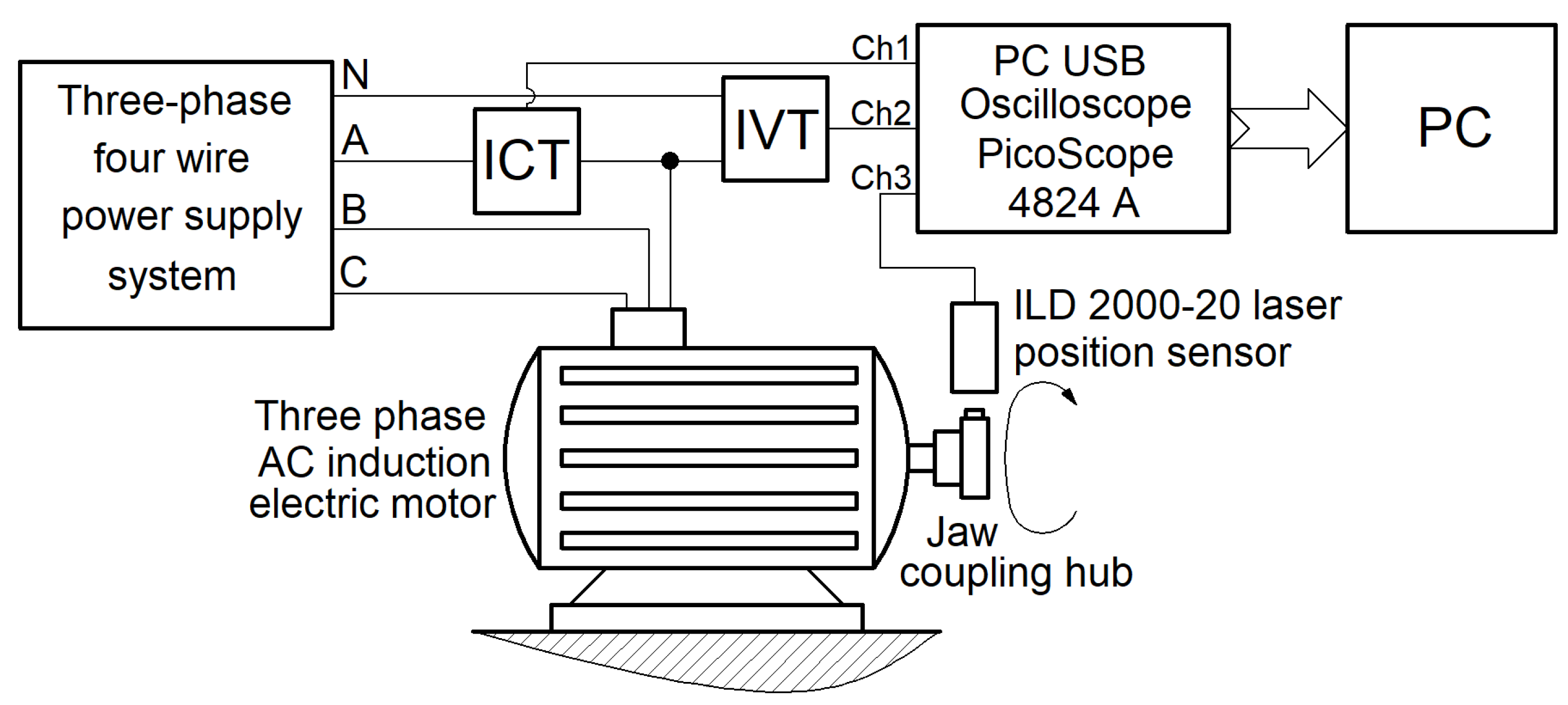
Figure 2.
A view on transformers ICT (1) and IVT (4), on digital oscilloscope (2) and personal computer (3).
Figure 2.
A view on transformers ICT (1) and IVT (4), on digital oscilloscope (2) and personal computer (3).
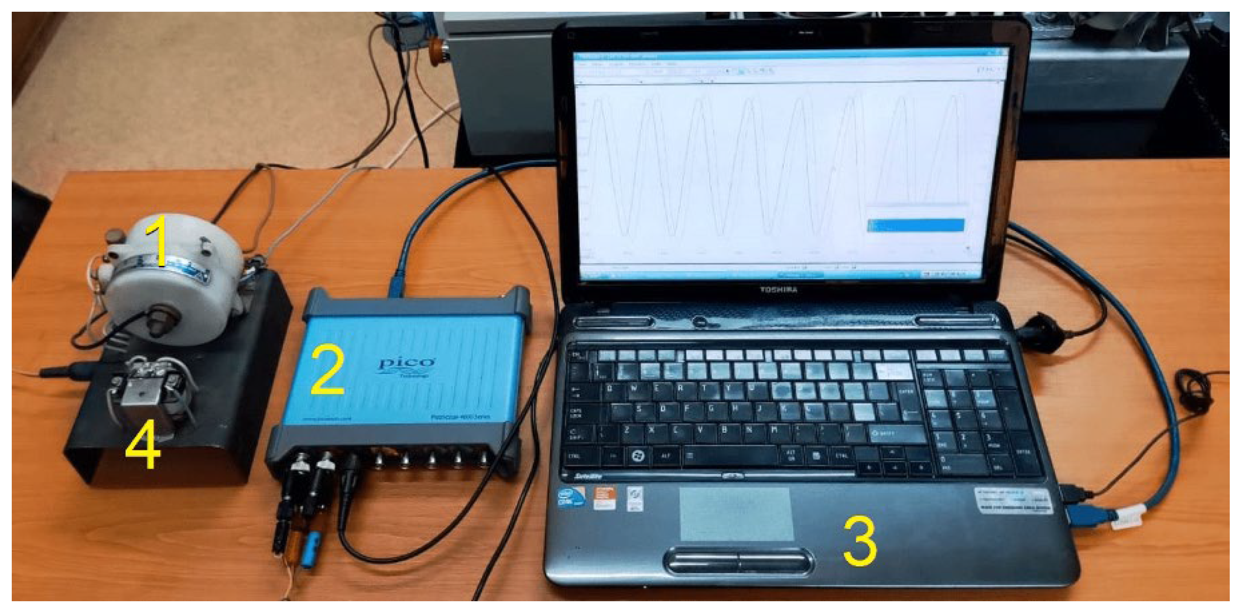
Figure 3.
A view on the jaw coupling hub placed on the motor rotor.
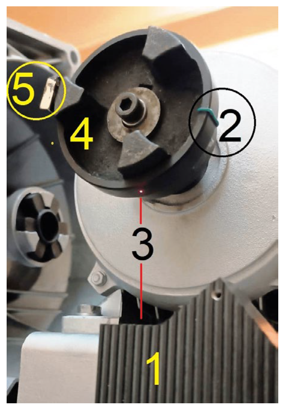
Figure 4.
A partial evolution of signals: 1- uVT(t); 2 – uCT(t); 3 – uSL(t). A, B – two successive passes of the angular marker 2 through the angular rotation origin 3.
Figure 4.
A partial evolution of signals: 1- uVT(t); 2 – uCT(t); 3 – uSL(t). A, B – two successive passes of the angular marker 2 through the angular rotation origin 3.
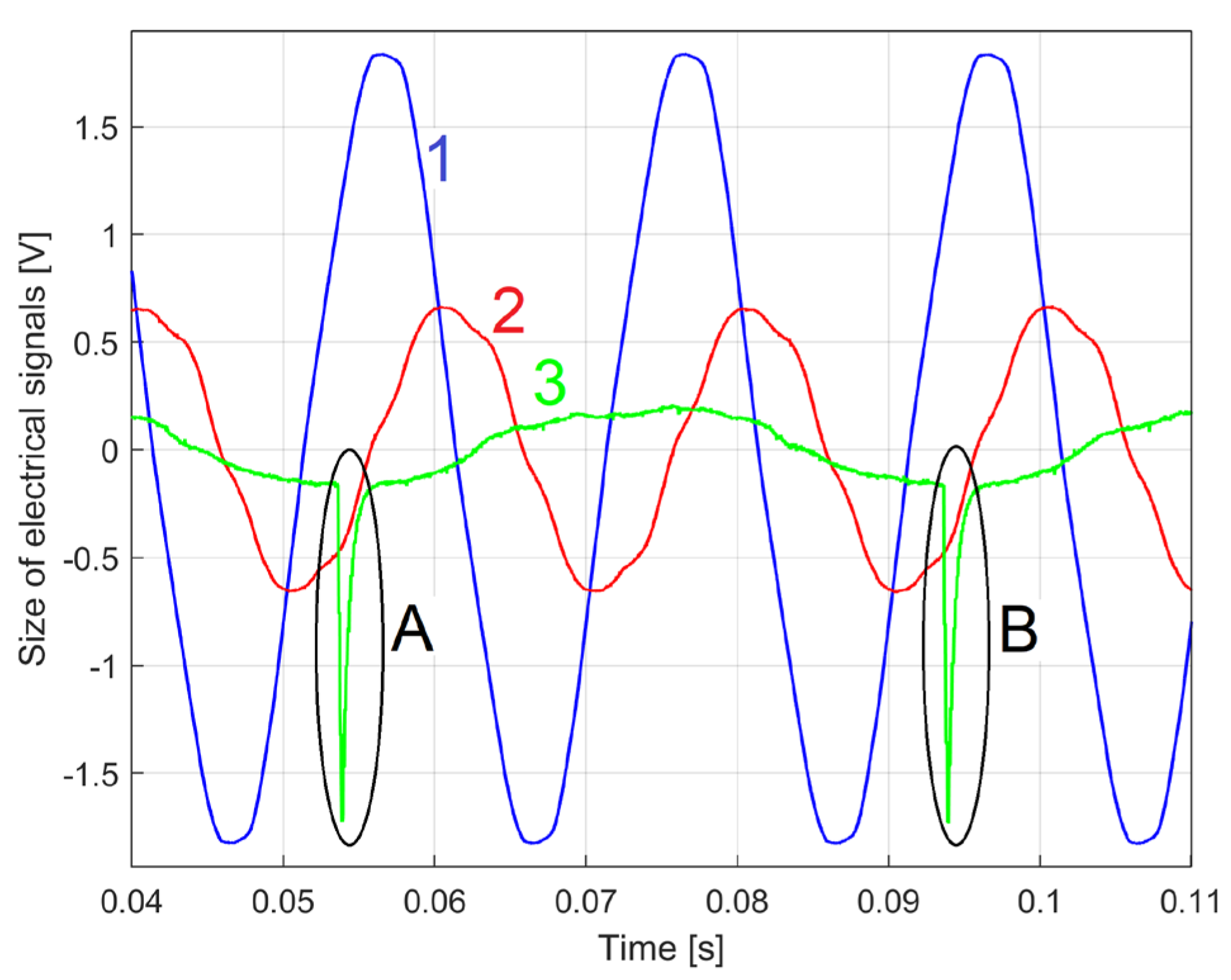
Figure 5.
A part of the FFT spectrum of IEP (in purple), a part of the transmission curve of an appropriate backward moving average filter used to extract the IAEP from IEP (in red).
Figure 5.
A part of the FFT spectrum of IEP (in purple), a part of the transmission curve of an appropriate backward moving average filter used to extract the IAEP from IEP (in red).
Figure 6.
A short sequence with the evolutions of: 1 – IAEPf; 2- IAEPc; 3 – IEP. .
Figure 7.
The evolution of a simulated VIAEPf signal (described mathematically by Equation (4)) with Δt=10μs and s=1÷2,000,000.
Figure 7.
The evolution of a simulated VIAEPf signal (described mathematically by Equation (4)) with Δt=10μs and s=1÷2,000,000.
Figure 8.
The pattern of a periodic component (with 33.5 Hz the fundamental frequency) within the simulated VIAEPf signal, found by FASS (in blue) superimposed on the simulated pattern (in red, Equation (5)).
Figure 8.
The pattern of a periodic component (with 33.5 Hz the fundamental frequency) within the simulated VIAEPf signal, found by FASS (in blue) superimposed on the simulated pattern (in red, Equation (5)).
Figure 9.
A sequence of uSL[s·Δt] signal, involved in the determination of the IAS value and the angular origin of the rotor.
Figure 9.
A sequence of uSL[s·Δt] signal, involved in the determination of the IAS value and the angular origin of the rotor.
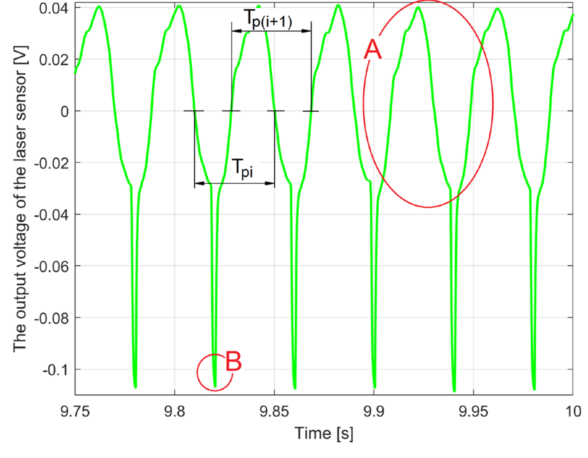
Figure 10.
The evolution of the IAEPf during a no-load test at 750 rpm theoretical synchronous speed.
Figure 10.
The evolution of the IAEPf during a no-load test at 750 rpm theoretical synchronous speed.
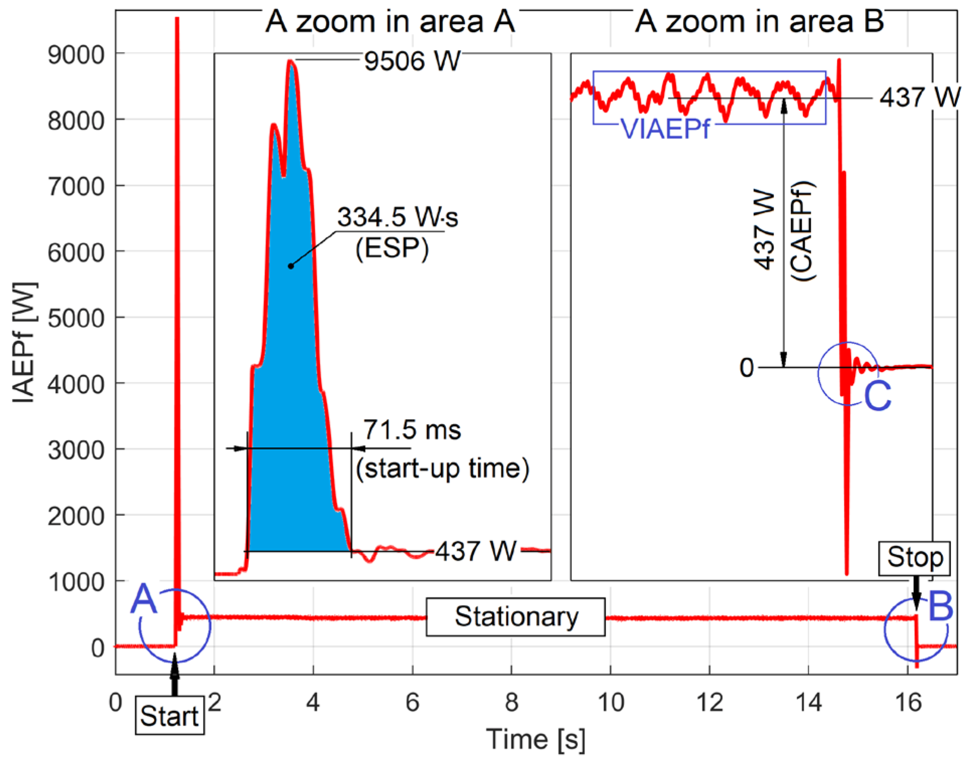
Figure 11.
The evolution of the IAEPf during a no-load test at 1500 rpm theoretical synchronous speed.
Figure 11.
The evolution of the IAEPf during a no-load test at 1500 rpm theoretical synchronous speed.
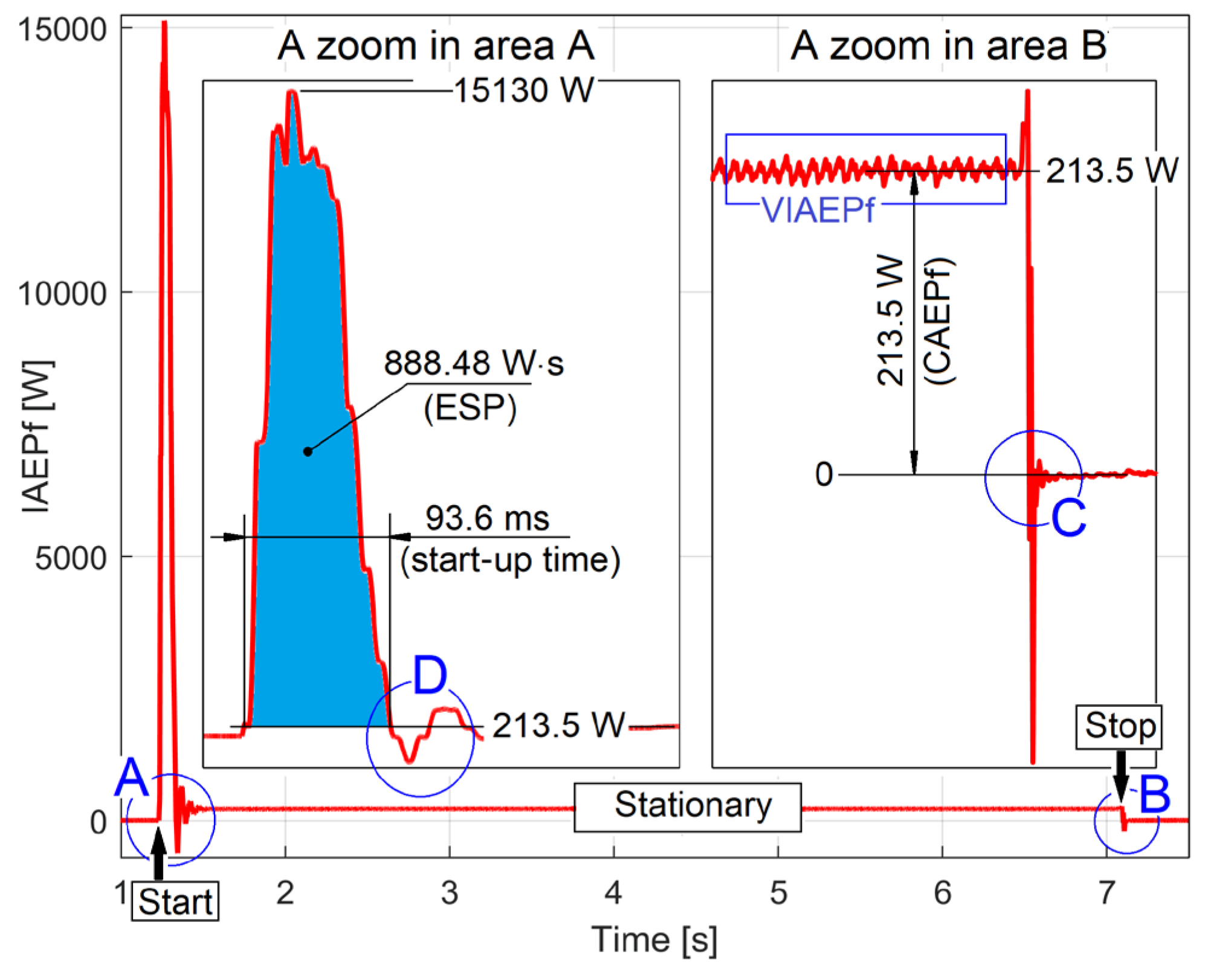
Figure 12.
. A zoomed-in detail in region D of Figure 11.
Figure 12.
. A zoomed-in detail in region D of Figure 11.
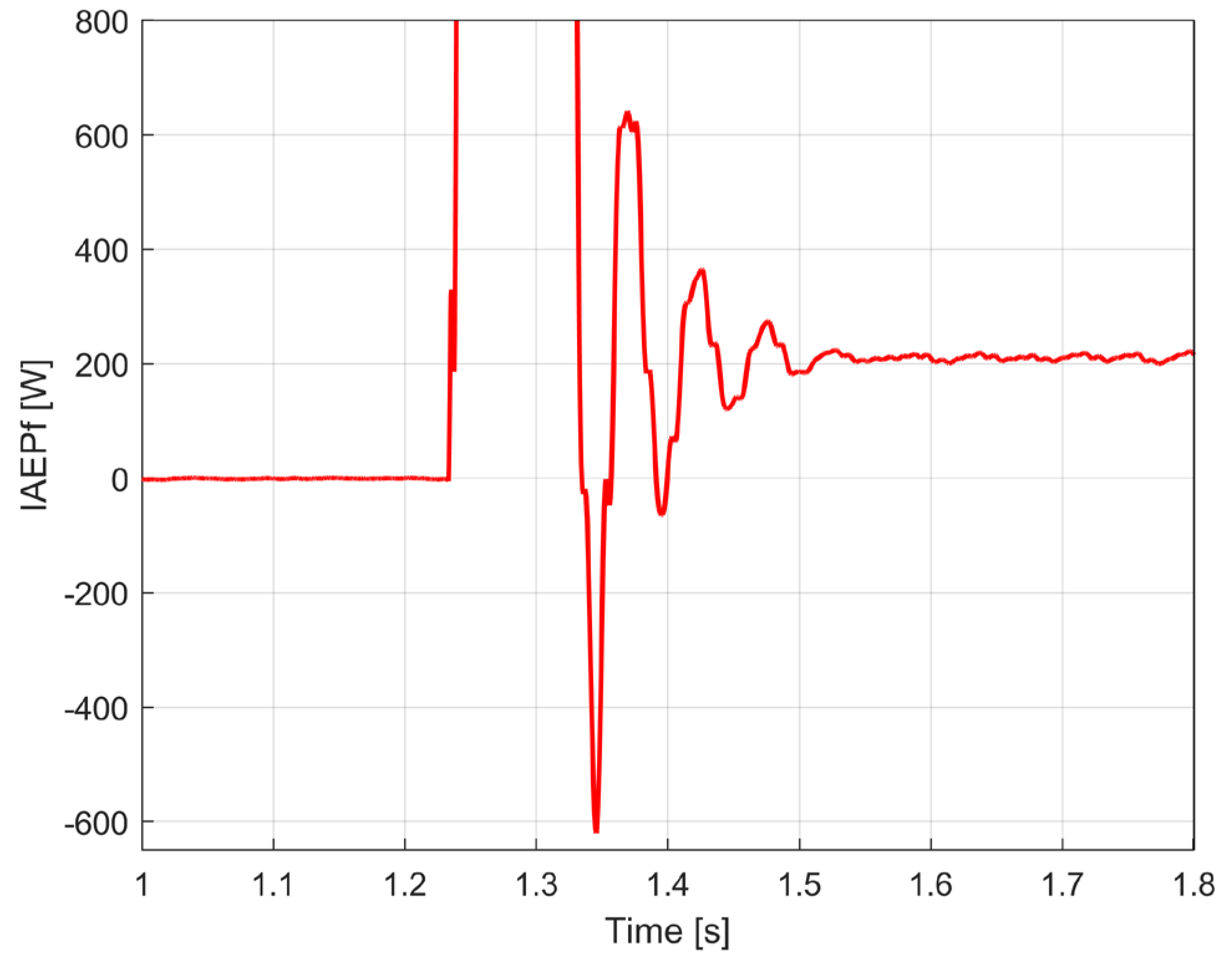
Figure 13.
The evolution of the rotor rotation frequency during a no-load stationary regime at the theoretical synchronous speed of 750 rpm.
Figure 13.
The evolution of the rotor rotation frequency during a no-load stationary regime at the theoretical synchronous speed of 750 rpm.
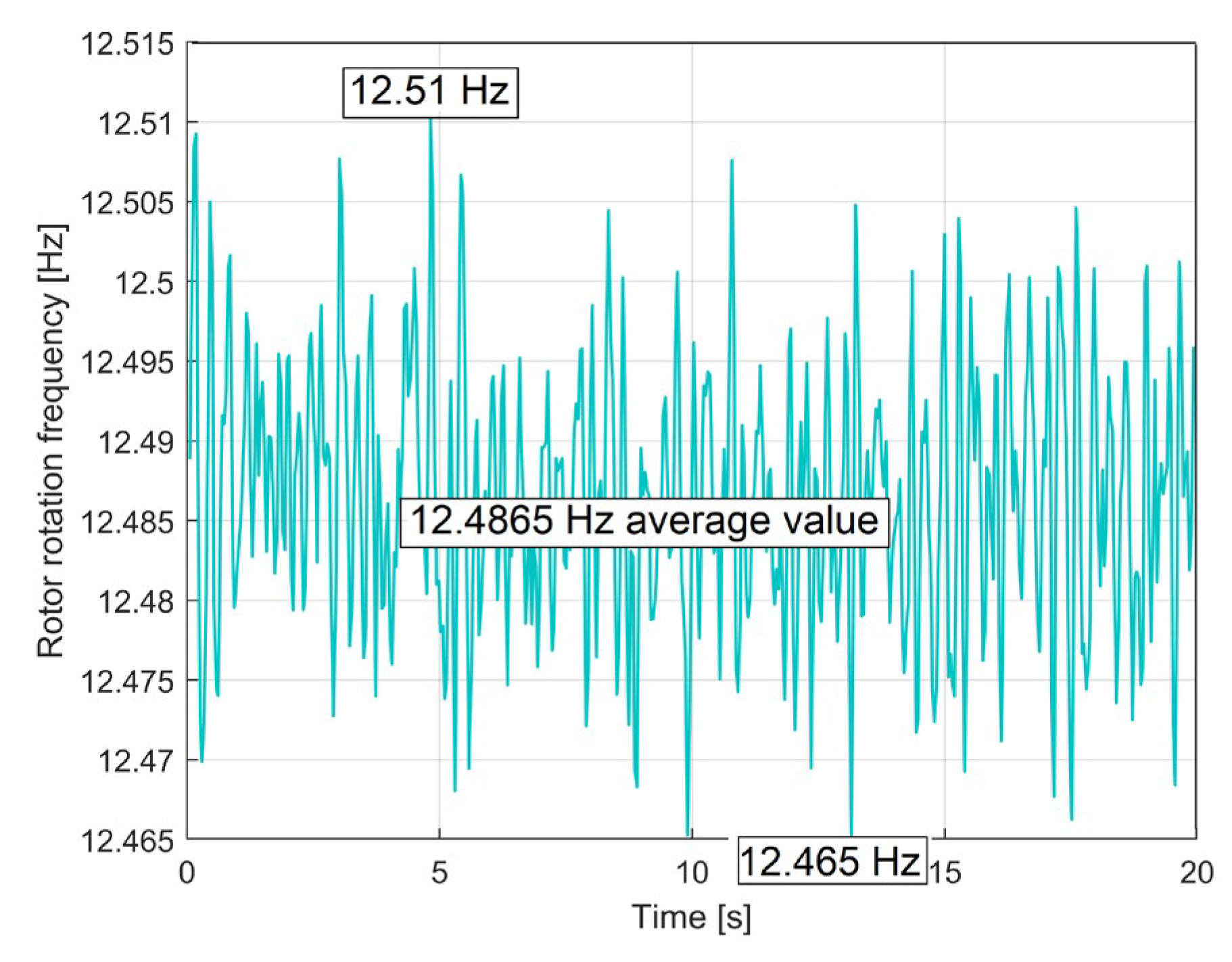
Figure 14.
The evolution of the IV frequency during the same stationary regime at the theoretical synchronous speed of 750 rpm.
Figure 14.
The evolution of the IV frequency during the same stationary regime at the theoretical synchronous speed of 750 rpm.
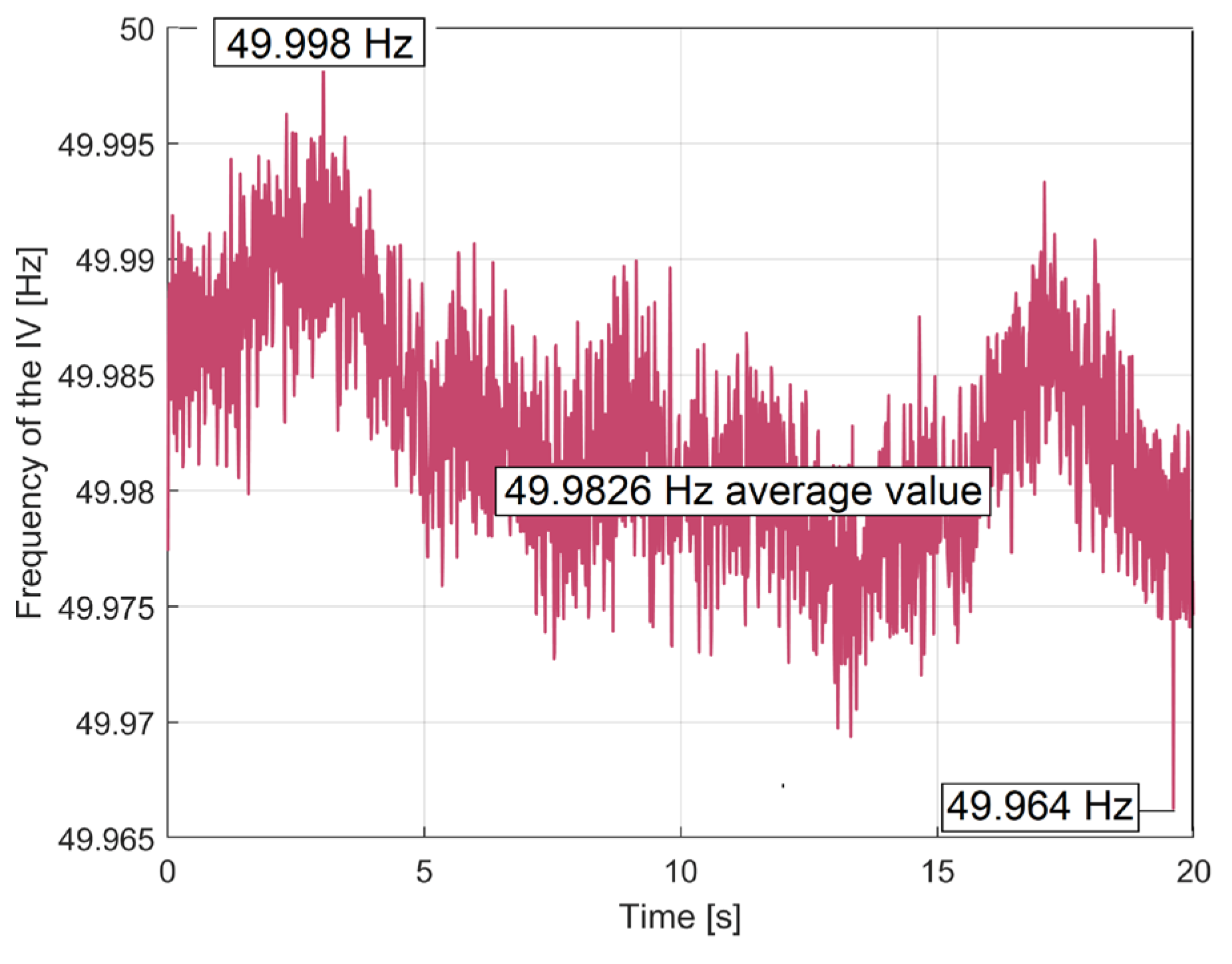
Figure 15.
The evolution of VIAEPf1 during a first experiment with the motor running at no-load (at 750 rpm theoretical synchronous speed), used to extract the PCRRf1a pattern by FASS.
Figure 15.
The evolution of VIAEPf1 during a first experiment with the motor running at no-load (at 750 rpm theoretical synchronous speed), used to extract the PCRRf1a pattern by FASS.
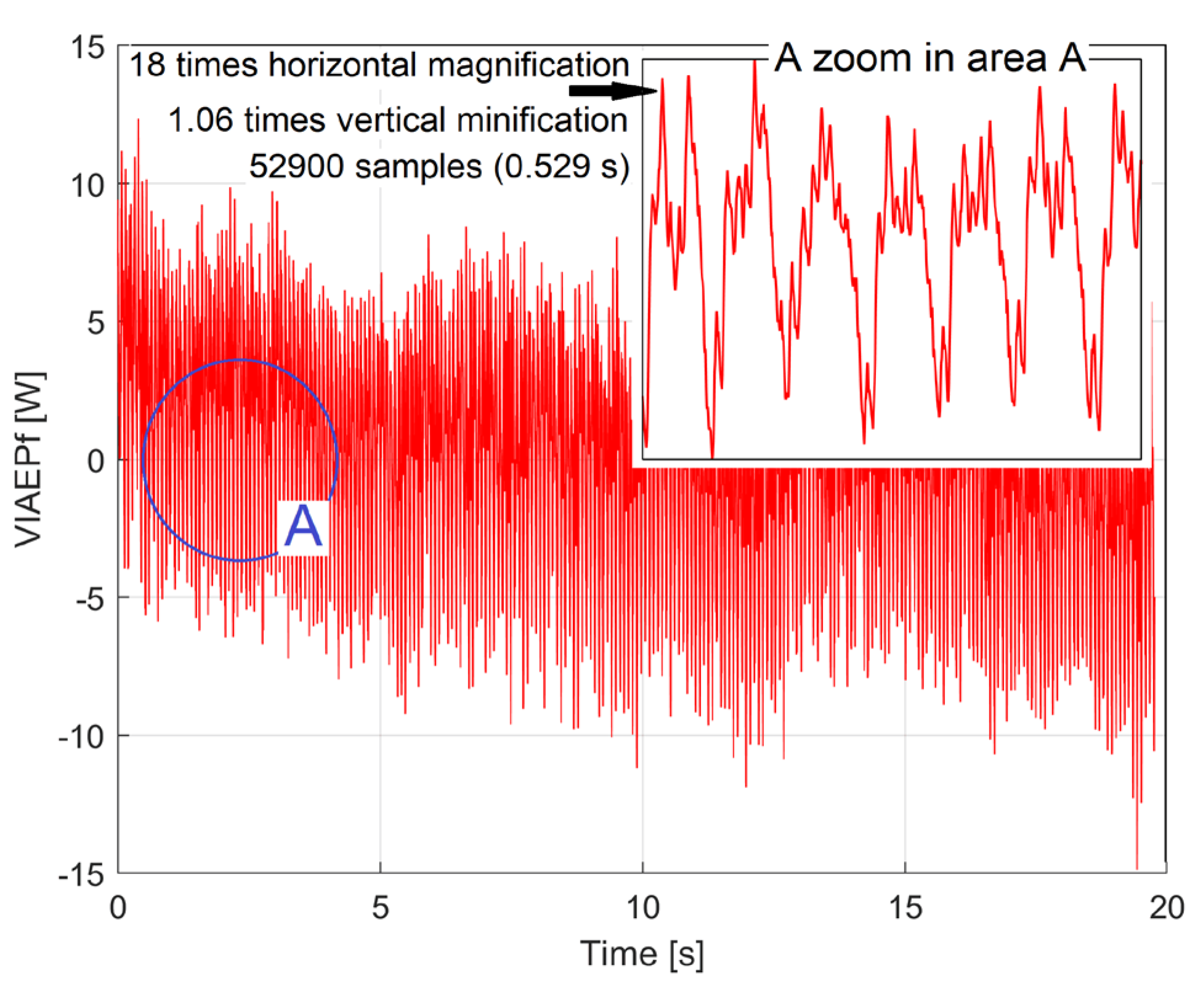
Figure 16.
A representation of two periods from PCRRf1a pattern (1), PCSL1a pattern (2) and PCRRf1b pattern (3).
Figure 16.
A representation of two periods from PCRRf1a pattern (1), PCSL1a pattern (2) and PCRRf1b pattern (3).
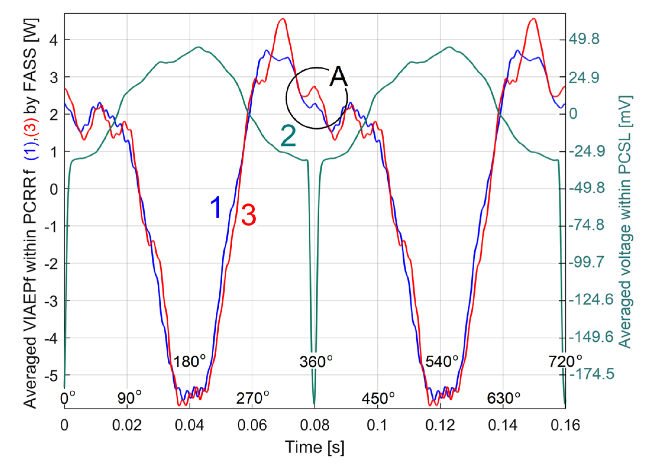
Figure 17.
A magnified view of Figure 16 in area A.
Figure 17.
A magnified view of Figure 16 in area A.
Figure 18.
PCRR1 patterns obtained without DUM (curve 1) and with three different angular positions of DUM on the jaw coupling hub (curves 2, 3 and 4).
Figure 18.
PCRR1 patterns obtained without DUM (curve 1) and with three different angular positions of DUM on the jaw coupling hub (curves 2, 3 and 4).
Figure 19.
Representation of PCRRf1a patterns (on two periods): 1- with synthetic definition (by FASS); 2- with analytical definition (using Equation (6) with r=15, found by curve fitting); 3- the difference between these patterns (as residual).
Figure 19.
Representation of PCRRf1a patterns (on two periods): 1- with synthetic definition (by FASS); 2- with analytical definition (using Equation (6) with r=15, found by curve fitting); 3- the difference between these patterns (as residual).
Figure 20.
1- The partial FFT spectrum of the synthetic PCRRf1a extended pattern (10 periods); 2 – A zoom in area A; 3 – A zoom in area B.
Figure 20.
1- The partial FFT spectrum of the synthetic PCRRf1a extended pattern (10 periods); 2 – A zoom in area A; 3 – A zoom in area B.
Figure 21.
1- The partial FFT spectrum of the analytical PCRRf1a extended pattern (10 periods); 2 – The lower part of the curve of the inverse transmissibility of the BMAF filter (1/Tr(f)) used to obtain IAEPf from IEP.
Figure 21.
1- The partial FFT spectrum of the analytical PCRRf1a extended pattern (10 periods); 2 – The lower part of the curve of the inverse transmissibility of the BMAF filter (1/Tr(f)) used to obtain IAEPf from IEP.
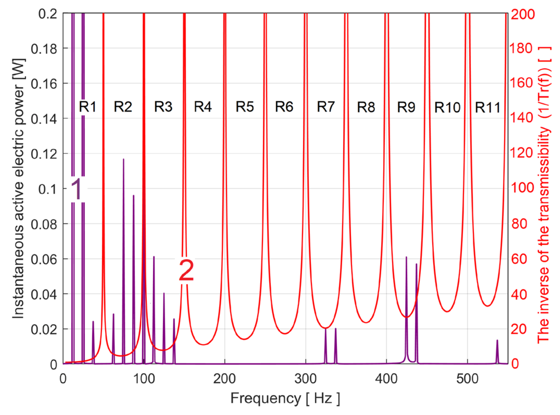
Figure 22.
Graphical descriptions of two periods from: 1 – the analytical PCRR1a pattern; 2 – the analytical PCRRf1a pattern.
Figure 22.
Graphical descriptions of two periods from: 1 – the analytical PCRR1a pattern; 2 – the analytical PCRRf1a pattern.
Figure 23.
Graphical descriptions of two periods from: 1 – the analytical PCRR1a pattern; 2 – the analytical PCRR1b pattern.
Figure 23.
Graphical descriptions of two periods from: 1 – the analytical PCRR1a pattern; 2 – the analytical PCRR1b pattern.
Figure 24.
The evolution of VIAEPf2a during a first test (without DUM) with the motor running at no-load (at 1500 rpm theoretical synchronous speed) used to extract the PCRRf2a pattern by FASS.
Figure 24.
The evolution of VIAEPf2a during a first test (without DUM) with the motor running at no-load (at 1500 rpm theoretical synchronous speed) used to extract the PCRRf2a pattern by FASS.
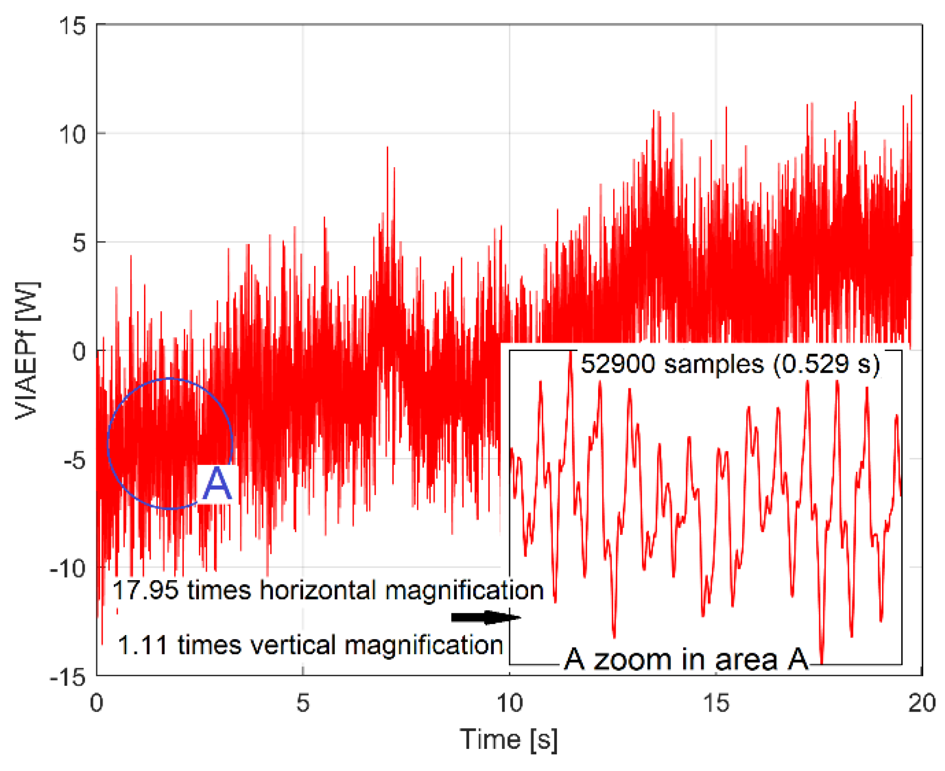
Figure 25.
A graphical representation with two periods of the patterns: 1 – PCRRf2a; 2 – PCRRf2b; 3 - PCRRf2c; 4 – overlaid PCSL2a, b, c.
Figure 25.
A graphical representation with two periods of the patterns: 1 – PCRRf2a; 2 – PCRRf2b; 3 - PCRRf2c; 4 – overlaid PCSL2a, b, c.
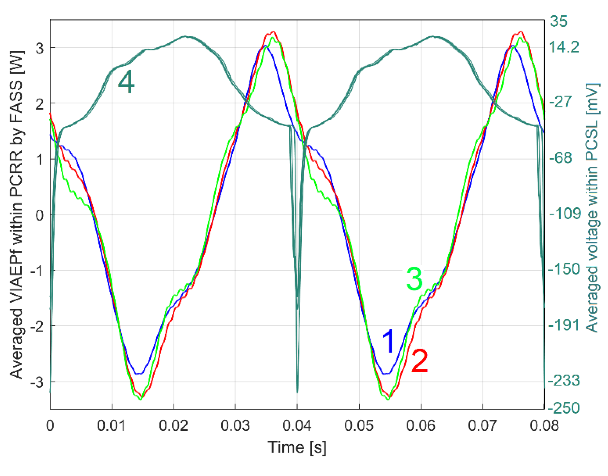
Figure 26.
The effect of the DUM placed on the jaw coupling hub at 60 degrees before the angular marker. A graphical representation with two periods of the patterns: 1 – PCRRf2a1; 2 – PCRRf2b1; 3 - PCRRf2c1; 4 –PCSL2a1; 5 – PCRRf2a.
Figure 26.
The effect of the DUM placed on the jaw coupling hub at 60 degrees before the angular marker. A graphical representation with two periods of the patterns: 1 – PCRRf2a1; 2 – PCRRf2b1; 3 - PCRRf2c1; 4 –PCSL2a1; 5 – PCRRf2a.
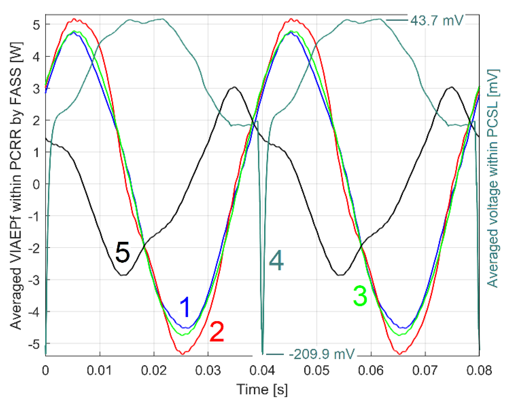
Figure 27.
The effect of the DUM placed on the jaw coupling hub at 60 degrees behind the angular marker. A graphical representation with two periods of the patterns: 1 – PCRRf2a2; 2 – PCRRf2b2; 3 - PCRRf2c2; 4 –PCSL2a2; 5 – PCRRf2a (from Figure 25); 6 – PCRRf2a1 (from Figure 26);
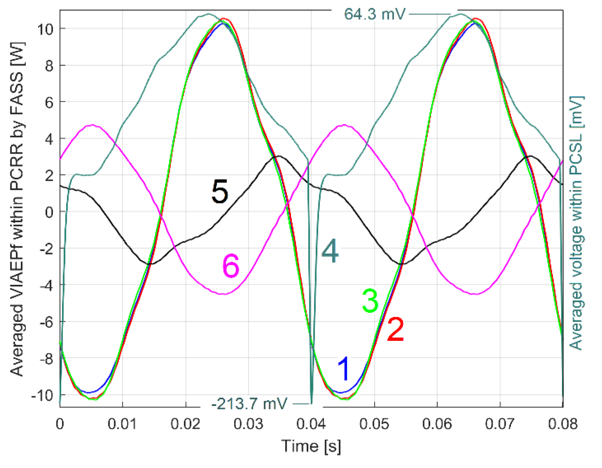
Figure 28.
A graphical representation with two periods of the patterns: 1 – PCRRf2a3; 2 – PCRRf2b3; 3 - PCRRf2c3; 4 –PCSL2a3; 5 – PCRRf2a (from Figure 25); 6 – PCRRf2a1 (from Figure 26); 7 – PCRRf2a2 (from Figure 27);.
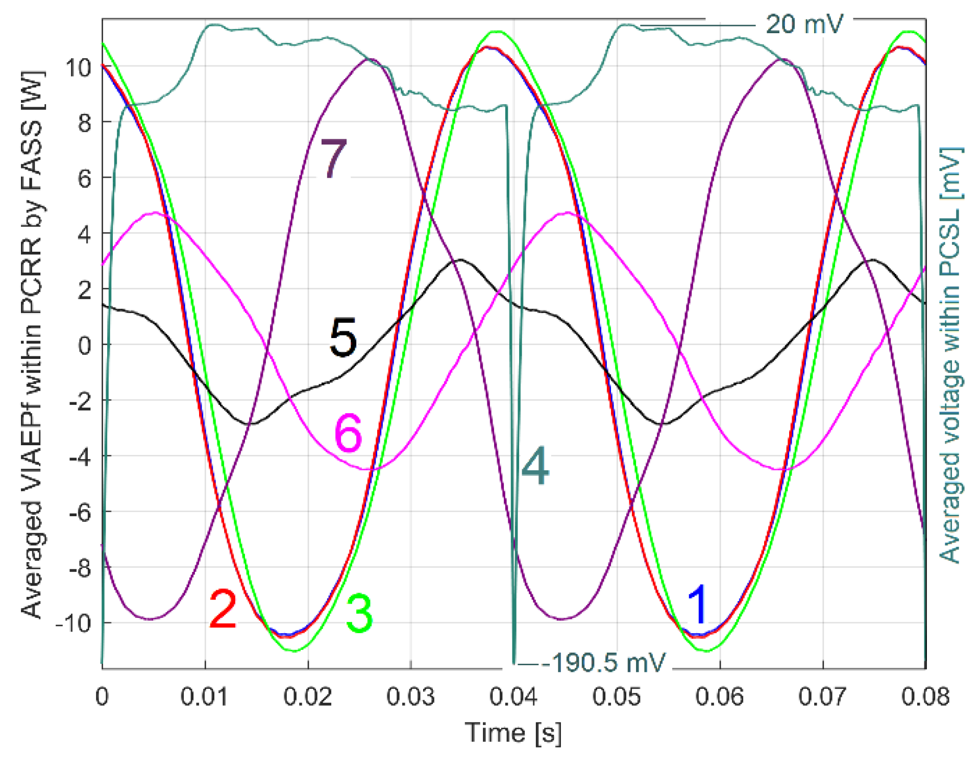
Figure 29.
A graphical representation with two periods of the patterns: 1 - PCRRf2a; 2 – PCRRf2a1; 3 – PCRRf2a2; 4 - PCRRf2a3; 5 – PCSL2a3.
Figure 29.
A graphical representation with two periods of the patterns: 1 - PCRRf2a; 2 – PCRRf2a1; 3 – PCRRf2a2; 4 - PCRRf2a3; 5 – PCSL2a3.
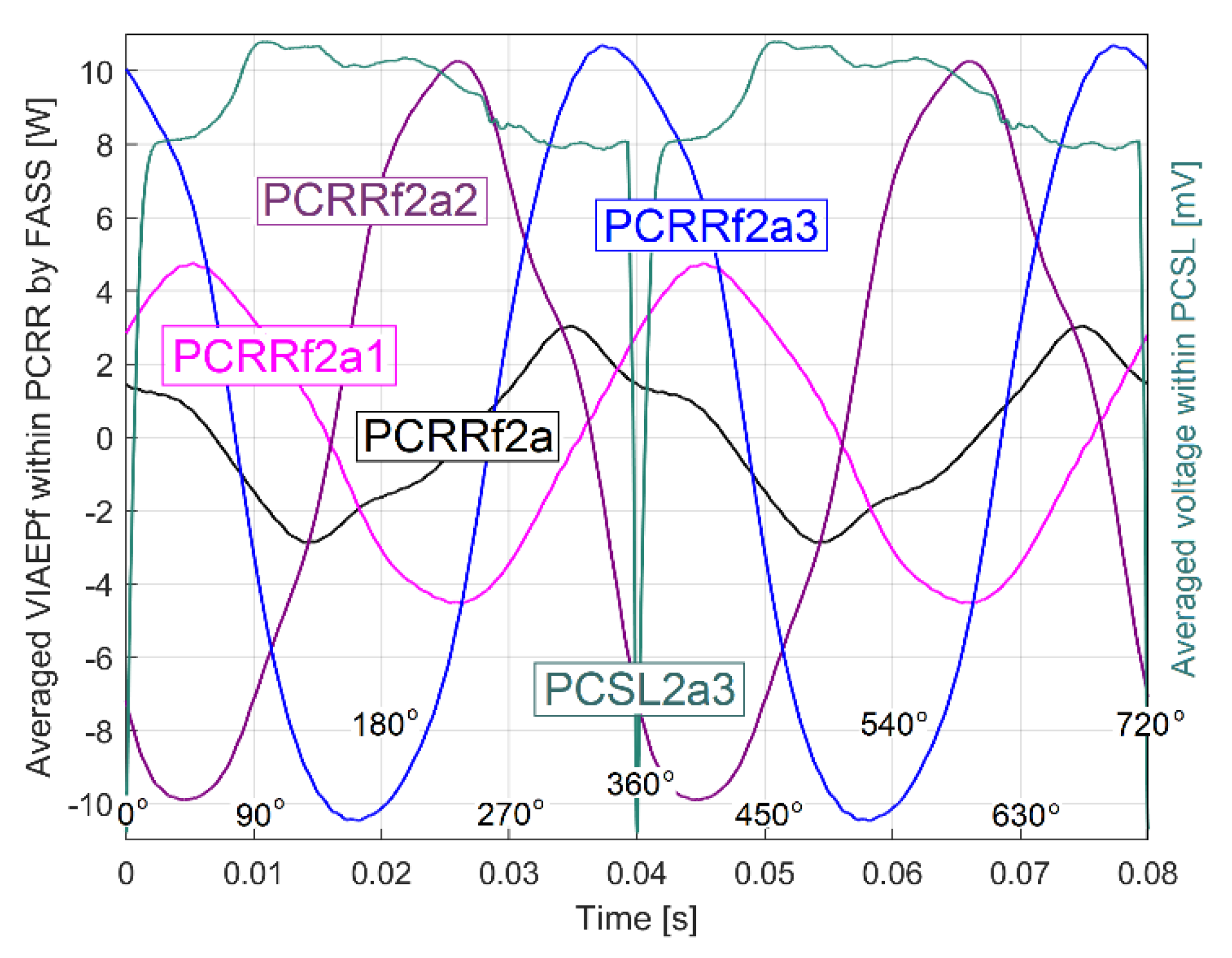
Figure 30.
The signals processing flow chart with some additional information.
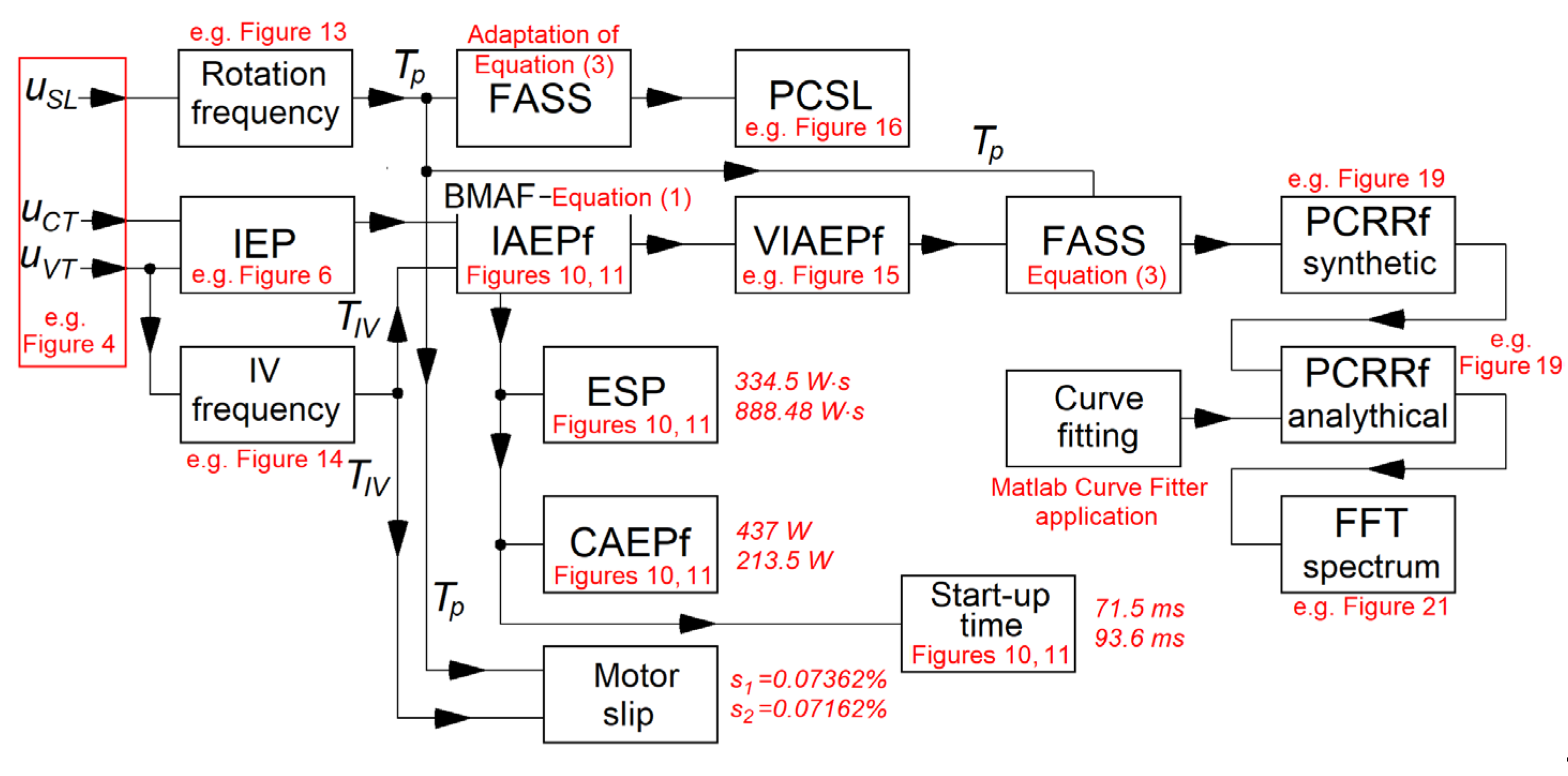

Table 1.
The values of the constants Afai, Bfai and Cfai involved in the analytical description of the PCRRf1a pattern, using Equation (6).
Table 1.
The values of the constants Afai, Bfai and Cfai involved in the analytical description of the PCRRf1a pattern, using Equation (6).
| i | Afai [W] |
Bfai [Hz] |
Cfai [rad] |
|
| 1 | 3.945 | 12.4857 = 1/Tp1a = Bfa1 | Fundamental | 1.725 |
| 2 | 1.913 | 24.9714 = 2· Bfa1 | 1st harmonic | -1.747 |
| 3 | 0.02436 | 37.4491 = 2.9993· Bfa1 | 2rd harmonic | 1.059 |
| 4 | 0.02832 | 62.4364 = 5.0006· Bfa1 | 4th harmonic | -2.031 |
| 5 | 0.1168 | 74.9142 = 6· Bfa1 | 5th harmonic | 2.07 |
| 6 | 0.09591 | 87.4078 =7· Bfa1 | 6th harmonic | -1.45 |
| 7 | 0.1688 | 99.8856 = 8· Bfa1 | 7th harmonic | 0.9121 |
| 8 | 0.06114 | 112.3474 =8.9980 · Bfa1 | 8th harmonic | 1.169 |
| 9 | 0.04019 | 124.8570 =10· Bfa1 | 9th harmonic | 0.5538 |
| 10 | 0.02553 | 137.3507 = 11· Bfa1 | 10th harmonic | 1.596 |
| 11 | 0.02038 | 324.6760 = 26· Bfa1 | 25th harmonic | 2.634 |
| 12 | 0.02024 | 337.0901 = 26.9980· Bfa1 | 26th harmonic | 1.23 |
| 13 | 0.06175 | 424.6253 = 34.0089· Bfa1 | 33th harmonic | -2.366 |
| 14 | 0.05657 | 437.0394 = 35.0032· Bfa1 | 34th harmonic | 1.26 |
| 15 | 0.01367 | 536.8296 = 42.9955· Bfa1 | 42th harmonic | -0.5324 |
Table 2.
The values of the constants Aai, Bai and Cai involved in the analytical description of the PCRR1a pattern, using Equation (6).
Table 2.
The values of the constants Aai, Bai and Cai involved in the analytical description of the PCRR1a pattern, using Equation (6).
| i | Afai [W] | 1/Tr(Bfai) | Aai = Afai·1/Tr(Bfai) [W] |
Bai [Hz] |
Cai [rad] |
|
| 1 | 3.945 | 1.103 | 4.351 | 12.4857 | Fundamental | 1.725 |
| 2 | 1.913 | 1.568 | 2.999 | 24.9714 | 1st harmonic | -1.747 |
| 3 | 0.02436 | 3.311 | 0.0807 | 37.4491 | 2rd harmonic | 1.059 |
| 4 | 0.02832 | 5.578 | 0.1580 | 62.4364 | 4th harmonic | -2.031+π=1.105 |
| 5 | 0.1168 | 4.704 | 0.5494 | 74.9142 | 5th harmonic | 2.07+π=5.2115 |
| 6 | 0.09591 | 7.697 | 0.7382 | 87.4078 | 6th harmonic | -1.45+π=1.6915 |
| 7 | 0.1688 | 608 | 102.6304 | 99.8856 | 7th harmonic | 0.9121 |
| 8 | 0.06114 | 10.111 | 0.6182 | 112.3474 | 8th harmonic | 1.169 |
| 9 | 0.04019 | 7.841 | 0.3151 | 124.8570 | 9th harmonic | 0.5538 |
| 10 | 0.02553 | 12.035 | 0.3073 | 137.3507 | 10th harmonic | 1.596 |
| 11 | 0.02038 | 20.398 | 0.4157 | 324.6760 | 25th harmonic | 2.634 |
| 12 | 0.02024 | 28.90 | 0.5849 | 337.0901 | 26th harmonic | 1.23 |
| 13 | 0.06175 | 26.684 | 1.6477 | 424.6253 | 33th harmonic | -2.366 |
| 14 | 0.05657 | 37.25 | 2.1072 | 437.0394 | 34th harmonic | 1.26 |
| 15 | 0.01367 | 45.09 | 0.6164 | 536.8296 | 42th harmonic | -0.5324 |
Disclaimer/Publisher’s Note: The statements, opinions and data contained in all publications are solely those of the individual author(s) and contributor(s) and not of MDPI and/or the editor(s). MDPI and/or the editor(s) disclaim responsibility for any injury to people or property resulting from any ideas, methods, instructions or products referred to in the content. |
© 2024 by the authors. Licensee MDPI, Basel, Switzerland. This article is an open access article distributed under the terms and conditions of the Creative Commons Attribution (CC BY) license (http://creativecommons.org/licenses/by/4.0/).
Copyright: This open access article is published under a Creative Commons CC BY 4.0 license, which permit the free download, distribution, and reuse, provided that the author and preprint are cited in any reuse.


