

Submitted:
10 June 2024
Posted:
11 June 2024
You are already at the latest version
Abstract
This paper presents the design of a robust speed controller for brushless DC motors (BLDCM) under field-oriented control (FOC). The proposed robust controller integrates extension theory (ET) and sliding mode theory (SMT) to achieve robustness. First, the speed difference between the speed command and the actual speed of the BLDCM, along with the rate of change of the speed difference, are divided into 20 interval categories. Then, the feedback speed difference and the rate of change of the speed difference are calculated for their extension correlation with each of the 20 interval categories. The interval category with the highest correlation is used to determine the appropriate control gain for the sliding mode speed controller. This gain adjustment tunes the parameters of the sliding surface in the SMT, thereby suppressing the overshoot of the motor speed. Because the sliding surface reaching law of the sliding mode controller (SMC) adopts the exponential approach law, the system's speed response can quickly follow the speed command in any state and exhibit excellent load regulation response. The simplicity of this robust control method, which requires minimal training data, facilitates easy implementation. Finally, the speed control of the BLDCM is simulated using Matlab/Simulink software, and the results are compared with those of the SMC using the constant speed approach law. The simulation results demonstrate that the proposed robust controller exhibits superior speed command tracking and load regulation response compared to the traditional SMC.
Keywords:
extension theory
; robust controller
; brushless DC motor
; field-oriented control
; sliding mode controller
; constant speed approach law
; exponential approach law
1. Introduction
In recent years, the increasing demand for motor drive performance and efficiency in industrial applications has led to the widespread adoption of permanent magnet synchronous motors (PMSM) [1]. Within PMSMs, brushless DC motors (BLDCM) [2] are widely utilized in industry due to their high torque, compact size, and high efficiency. Given the stringent requirements for precision in speed and position control, field-oriented control (FOC) [3] is commonly employed for speed and position regulation.
In the traditional FOC architecture, three proportional-integrated (P-I) controllers [4] are required, including a speed controller, a d-axis current controller, and a q-axis current controller. While these three controllers are relatively straightforward to design, significant variations in speed commands or load changes can adversely affect the performance of traditional P-I controllers. Therefore, numerous robust controllers have been introduced to improve control performance. However, these intelligent controllers face various challenges. For instance, sliding mode controllers (SMC) [5] tend to exhibit overshoot, while extension controllers [6] may face stability concerns if the operating point falls outside the neighborhood domain. Additionally, fuzzy controllers [7] often suffer from excessively long computation times. Additionally, from a practical implementation perspective, existing intelligent controllers are relatively difficult to realize and often fail to achieve the expected control performance. For example, controllers that combine fuzzy theory with sliding mode theory (SMT) [8] are particularly challenging to implement effectively. In contrast, the controller proposed in this paper requires relatively less computation, thereby reducing the computational load on the digital signal processor. Additionally, due to its simple program structure, the controller parameters can be easily modified through programming to enhance system stability and robustness. This makes it well-suited for speed control of BLDCMs under varying speed commands and significant load changes.
The control strategy proposed in this paper is based on ET [9] to determine the appropriate SMC gains, thereby altering the structure of the sliding mode function for faster and more stable sliding mode control response. First, the speed error between the motor’s speed command and its actual speed, along with the rate of change of the speed error, are used as features for ET. These features are divided into 20 interval categories based on their magnitude. The classical domain and neighborhood domain of ET are then used to establish an extension matter element model. The weights of the speed error and its rate of change are set according to their importance. The correlation degree between the speed error, its rate of change, and the interval categories are then calculated. The category with the highest correlation degree is selected, and the corresponding sliding mode function control gain is output. This gain modifies the sliding mode controller’s sliding surface function so that the original sliding surface function no longer has a fixed slope. Thus, by using ET to determine the gain of the sliding surface function and replacing the constant speed approach law of the SMC with an exponential approach law, rapid speed command tracking can be achieved. This approach not only optimizes the stability of the sliding surface but also mitigates the overshoot caused by the SMC. As a result, the motor’s speed response is not only faster but also more stable.
2. BLDCM System
The primary distinguishing feature of BLDCM compared to brushed DC motors is the absence of brushes for commutation. Instead, BLDCMs use electrical methods to detect the rotor position and control its speed. Therefore, magnetic components (Hall sensors) or optical encoders [10] must be integrated into the motor’s axis to provide feedback on the rotor’s position to the controller. This allows the controller to determine the current position of the motor rotor, serving as the basis for commutation control.
2.1. Mathematical Model of BLDCM
Establishing a mathematical model is a crucial step in the design of a controller for BLDCMs. Using the mathematical model of the motor as the core foundation, we can perform the analysis and judgment using ET and the modeling of the SMC. This mathematical model allows for the estimation of the controller parameter design values to determine whether the expected control performance can be achieved, thereby facilitating the design of the controller parameters.
Figure 1 depicts the three-phase equivalent circuit of a BLDCM within a stationary reference frame.
According to Kirchhoff’s voltage law, the relationship between the phase voltages and phase currents of a BLDCM can be expressed as Equation (1).
Where:
are the phase voltages of phases a, b, and c respectively.
are the stator resistances of phases a, b, and c respectively.
are the phase currents of phases a, b, and c respectively.
are the self-inductances of phases a, b, and c respectively.
are the mutual inductances between phases a, b, and c.
are the back electromotive forces (EMF) of phases a, b, and c respectively.
Assuming the motor is three-phase balanced, then
By substituting Equations (2) and (3) into Equation (1), we obtain
Since the motor is three-phase balanced, therefore ian+ ian+ian=0, we obtain
Substituting Equation (5) into Equation (4), we obtain the state equation of the BLDCM as shown in Equation (6).
Since the speed of the BLDCM is proportional to the back EMF, and the input current is proportional to the torque, the electromagnetic torque Te can be derived using the three-phase currents, back EMF, and rotor speed, as shown in Equation (7).
Where:
The electromagnetic torque generated by the motor.
The mechanical speed of the motor.
The mechanical equation of the BLDCM can be expressed as:
Where:
Represents the load torque.
Represents the rotational inertia of the motor and load.
Represents the coefficient of viscous friction of the motor and load.
2.2. Dynamic Equations of the FOC System for BLDCMs
FOC finds widespread application in motor drive systems, enabling both motor speed and position control with the same architecture. To implement FOC, it is necessary to detect the rotor position of the motor first, and then provide the switching control signals to the inverter [11] through coordinate transformation. However, in the implementation process, analyzing the three-axis spatial coordinate system of a three-phase motor directly can be computationally challenging. Therefore, it is necessary to perform a coordinate transformation [12] to convert the original three-axis spatial coordinates into a two-axis spatial coordinate representation, making the calculations simpler and easier to implement. Hence, this section will focus on spatial coordinate transformation to explain the principles of FOC systems.
Under ideal conditions, the voltage equation of a BLDCM in a three-phase synchronous stationary coordinate system is represented by Equation (9) [13].
Where:
Stator resistance of the three phases.
Magnetic fluxes of phases a, b, and c, respectively.
The magnetic flux of a BLDCM is generated by the combination of the current passing through the stator windings and the permanent magnets on the rotor. Under ideal conditions, the magnetic field generated by the permanent magnets has a constant amplitude, indicating that the rotor’s relative position is fixed. Therefore, this magnetic field can be represented by a vector . The position of the stator is determined by the angle between the direction of the magnetic field orientation and the stator coordinate system. The flux is the projection of a constant flux vector along the axis direction. The magnetic flux equation in the three-phase stationary coordinate system is represented as Equation (10).
Where:
M: is the mutual inductance between phase windings.
is the self-inductance of each phase winding.
is the flux produced by the permanent magnets.
is the angle between the rotor pole and the axis of the phase winding.
is the synchronous speed of the motor.
The three-phase stationary coordinate system can be transformed into a two-phase stationary coordinate system through the Clarke transformation, as shown in Equation (11).
The magnetic flux equation can be expressed as Equation (12).
By differentiating the magnetic flux Equation (12) and substituting it into Equation (11), the voltage equations for the two-phase stationary coordinate system can be obtained, as shown in Equation (13).
After applying the Park transformation to the two-phase stationary coordinate system, two dependent equations can be derived in the two-phase synchronous rotating coordinate system, as shown in Equation (14). The magnetic flux equations are then represented as shown in Equation (15).
From Equation (15), the torque equation for the two-phase synchronous rotating system can be derived, as shown in Equation (16).
The torque equation for the two-phase synchronous rotating system can be formulated as Equation (17).
If the FOC method is adopted, we can set . Then, the voltage equations can be simplified to Equations (18) and (19).
From Equation (16), the torque equation can be expressed as Equation (20).
Where is the torque constant, and P is the number of poles. Using Equation (8), the motion equation for the BLDCM can be expressed as Equation (21)
The equation derived from Equation (20) reveals that when employing FOC, controlling can regulate torque magnitude. Moreover, as shown in Equation (19), the axis voltage is solely related to , effectively simplifying the control requirements for the BLDCM system architecture. When , it can be regarded as a separately excited DC motor, where the stator has only the quadrature ( axis) component, and the spatial vector of the stator magnetic flux coincides orthogonally with the spatial vector of the permanent magnet field. Figure 2 illustrates the block diagram of the FOC for the BLDCM.
3. Proposed Intelligent Algorithm for Drive Control
Due to the fixed parameter values of traditional P-I controllers, their control performance deteriorates when the speed command of the FOC system changes or when load variations occur, potentially leading to system divergence.
Therefore, this paper proposes a speed controller that integrates ET with SMT, enabling the system to achieve faster speed response and possess self-adaptive capability [14]. The design process of the proposed intelligent controller that combines ET with SMC is described below.
3.1. Extension Theory
Extension Theory (ET) [6] was proposed by Chinese scholar Professor Cai Wen in 1983. It primarily explores the variability of things, examining the principles and methods for resolving contradictory problems from both qualitative and quantitative perspectives. The two core components of ET are matter element theory and extension mathematics. Matter element theory describes the possibilities of changes in things and the characteristics of matter element transformations, while extension mathematics relies on extension set and correlation function as the core of its calculations.
ET represents information about things through the matter element model. It expresses the transformation relationships between the qualitative and quantitative aspects of things via matter element transformations. By utilizing correlation functions for discrimination, the theory helps understand the influence of qualitative and quantitative factors on things, thereby clearly presenting the degree of impact on the characteristics of things.
3.1.1. Extension Matter Element Model
In ET, the representation of information about things is achieved by expressing the things in terms of a matter element model, using a mathematical function as shown in Equation (22).
Where:
The fundamental element describing an entity is referred to as matter element.
Denotes the name of the entity.
Represents the characteristics or features of the entity.
The value of the feature of the entity.
In ET, if the feature of the matter element is not a single feature, it is represented by features and their corresponding feature values. Therefore, the feature can be expressed as , and the feature values can be represented by . Therefore, extensional function of matter elements can transform Equation (22) into a matrix-vector form, represented as Equation (23).
3.1.2. Definition of Classical Domain and Neighborhood Domain in ET
If the value range of a feature is defined as its classical domain , and it is contained within a neighborhood domain , then . If point lies within an interval , the corresponding matter element can be expressed as Equation (24).
Where is the feature of , and is the feature value of . As for , the corresponding matter element can be expressed as Equation (25). In this expression, is the characteristic value of and is the characteristic quantity of .
3.1.3. Distance and Rank Value
In classical mathematics, the terms distance and rank value refer to the relationship between two points. However, in ET, these terms represent the distance relationship between a point in the real domain and an interval . Mathematically, this relationship can be expressed as Equation (26).
In addition to considering the relationship between a point and an interval, it is also necessary to consider the relationship between a point and two intervals. Thus, assuming and are two intervals in the real domain, and interval is contained within , the rank values of point , interval , and interval can be expressed as Equation (27).
3.1.4. Correlation Function
If , and , when the two intervals do not intersect at a common endpoint, their correlation function can be expressed as Equation (28).
In Equation (28), when , the function value reaches its maximum. Therefore, this correlation function can also be referred to as the elementary correlation function [15]. A schematic diagram is shown in Figure 3. Additionally, when , it indicates that point is outside the interval C. Conversely, when , it signifies that point is within the interval . However, if , it implies that point is located within the extension domain.
3.2. Sliding Mode Controller Design
While traditional P-I controllers can meet control performance requirements at specific operating points, their performance response is affected by load variations. Moreover, they are susceptible to changes in motor parameters and external disturbances, making them unsuitable for applications requiring high control performance. Furthermore, BLDCMs are nonlinear and strongly coupled multivariable systems. Consequently, to address the robustness [16] issues of traditional P-I controllers or their insufficient self-adaptive capability, several intelligent control algorithms have emerged.
The variable structure control of SMCs exhibits lower dependence on motor models and demonstrates robustness against external load variations, system disturbances, and internal parameter changes. As a result, it can effectively drive the system along a predefined sliding mode trajectory, making it widely applicable in speed regulation and load disturbance rejection control of BLDCMs.
3.2.1. State Variable Design
In order to replace the traditional field-oriented speed control loop with a P-I controller, the mathematical equations for the d-q axis of the BLDCM can be derived from the matrix Equations (14) and (15), as shown in Equation (29). Since the BLDC motor used in this study is a surface-mounted (SM) rotor type, its d and q-axis inductance values are equal, denoted as .
Due to the very small viscous friction coefficient, it can be neglected. Therefore, Equation (21) allows the motion equation for the SM rotor BLDCM to be simplified to Equation (30).
However, to achieve FOC, control strategy must be adopted. Therefore, Equation (31) can be derived from Equations (20), (29), and (30).
Since the goal is to apply the SMC to speed loop control, the input signal to the controller is the difference between the speed command and the actual feedback signal (i.e., the speed difference). The controller output is the q-axis command current aiming to achieve and ensure that the rate of change of the speed difference . Based on this, the state variables of the BLDCM system can be defined as shown in Equation (32).
By differentiating Equations (31) and (32), the rate of change of the state variables can be derived, as shown in Equation (33).
Let , then substituting it into Equation (33) for yields Equation (34).
3.2.2. Sliding Surface Design
In the SMC, the design objective of the controller is to ensure and . Therefore, the sliding surface function [17]can be expressed in the form of Equation (35).
Where:
sliding surface function.
control gain.
state variables.
When , and let , Equation (35) can be rewritten as Equation (36), and and can be solved, as shown in Equation (37).
Equation (37) reveals that over time, the values of the state variables and decay exponentially to 0. Therefore, when , which represents the designed sliding surface, and the sliding surface function reaches the sliding surface , the system’s state variables will approach 0, thus achieving the goal of state variable control.
3.2.3. Sliding Mode Approach Design
To ensure that the sliding surface function reaches at a certain time point (i.e., reaching the sliding surface) and remains stable, it is necessary to design an approaching law function [18].
From the design of the sliding surface, it is evident that to ensure , the output function of the BLDCM speed controller must be designed to meet the control requirements. Hence, Equation (35) can be reformulated as Equation (38).
Where, represents the sliding mode approaching law function.
Since is the output of the speed controller, the control force function is defined as , thereby transforming Equation (38) into Equation (39).
According to Lyapunov’s second stability criterion [19], if there exists a continuous function , it must satisfy the following three conditions:
Therefore, when the system is stable at the equilibrium point , it ensures that . Furthermore, if we let , not only can we satisfy Conditions (1) and (2) in Equation (40), but we can also deduce the third condition through analysis, as shown in Equation (41).
Next, we design the approaching law function such that . The common approaching law functions include the constant speed approaching law function and the exponential approaching law function, which can be respectively represented by Equations (42) and (43).
Where
According to the two approaching law functions mentioned above, when , from Equation (39), the controller’s can be obtained. This implies applying the control force function to the motor model. Thus, the final response will stabilize at the origin of the designed sliding surface.
3.2.4. Controller Output Design
According to the aforementioned reaching law design, it can be inferred that the first two conditions of the Lyapunov function ensure [20]. However, if the constant speed approaching law function given by Equation (42) is adopted, regardless of whether or (reaching the sliding surface) can satisfy the requirements of the Lyapunov function. However, due to its consistent response speed, attempting to expedite the response would result in oscillations on the sliding surface. Conversely, to stabilize it on the sliding mode surface, it would take a significantly longer time to reach the sliding mode surface. This intricate delay in response time certainly diminishes its practical applicability in real-world applications. From Equation (43), it can be observed that the exponential approach law [21] differs from the former by the addition of an exponential approach term . When the value of the exponential approach term is small (i.e., closer to the sliding surface), is approximately 0. Therefore, it is dominated by . Conversely, if this value is large (i.e., the approach distance is much greater than the sliding surface), the value of will also be larger. In this case, it is dominated by the exponential approach term, thereby enhancing the speed response of approaching the sliding surface, enabling the system to approach the sliding surface more quickly. Therefore, the exponential approach law is more suitable for systems experiencing significant parameter disturbances or large load variations.
In summary, compared to constant speed approach laws, the exponential approach law offers superior characteristics. Hence, the controller proposed in this paper adopts the exponential approaching law function for the sliding surface. However, it necessitates solving the exponential approach term ( ) from Equation (43). In Equation (43), where represents the exponential approach term, its solution is given by:
In Equation (44), represents the exponential term, thus Equation (43) is referred to as the exponential approaching law function.
The exponential approaching law function is the selected approaching law function in this paper. From Equation (39), it can be inferred that is the output of the controller. Therefore, defining the controller function as , Equation (39) can be rewritten as Equation (45).
Consequently, the expression for the control force function can be written as shown in Equation (46).
From Equation (46), it can be inferred that the commanded current of the axis can be represented as Equation (47).
3.3. Feature Selection for ET Integrated SMC of the Drive System
In order to achieve faster and more stable control response for the PNVF-90 BLDCM, ET is adopted in this paper for speed control. The control method involves partitioning the speed difference between the motor’s actual speed and the commanded speed, as well as the rate of change of speed difference , within the speed range into 20 intervals (i.e., 20 states). The relationship between these intervals is illustrated in Figure 4. From Figure 4, it can be observed that intervals A1 to A4 exhibit larger oscillations due to the significant differences in speed commands, while categories A17 to A20 show smaller oscillations as the speed difference is smaller. For interval A1, it is observed that , and increases continuously. Although >0, its value decreases over time, and at point . However, reaches its maximum value at this point. This indicates that when the speed difference is larger and the rate of change of speed difference is smaller, the control effort for speed control needs to be significantly reduced. This trend can be observed in other intervals as well. Therefore, according to ET, the dynamic analysis chart in Figure 4, characterized by the speed difference and the rate of change of speed difference, is used to establish classical domain matter element models for 20 intervals (as shown in Table 1). The control gain values corresponding to these 20 classical domain matter element models in the SMC are used to modify the dynamic model of the SMC. This adjustment alters the sliding surface function, enabling a faster transient response and suppressing the overshoot caused by the exponential approach law. Furthermore, the neighborhood domain is established using the maximum and minimum values of each feature’s classical domain, as shown in Equation (48).
3.4. Integration of ET and SMC for Speed Control
To achieve both stability and fast response in motor speed control, this study utilizes ET to calculate the correlation between the motor speed command and the actual speed difference, as well as the rate of change of the speed difference. Simultaneously, it completes the calculation of the sliding surface function for the sliding mode controller. Initially, ET is employed to identify the feature with the highest correlation, categorizing it into the most appropriate feature category interval. This process is crucial for determining the optimal control gain function for the SMC. The SMC utilizes an exponential approach law to enhance the motor speed response. The control process involves computing the correlation using ET to classify the motor speed features, thereby determining the stable control gain of the sliding surface. This is crucial for suppressing overshoot caused by the exponential approach law of the SMC.
The test motor used in this study is the PNVF-90 permanent magnet BLDCM. Due to its rated speed of , the speed range is set . The state variable characteristics of the ET and SMC are the speed difference between the commanded speed and the actual feedback speed, and the rate of change of the speed difference, denoted as and .
Therefore, based on the above analysis, the motor operating state is first determined using ET, which then decides the sliding mode controller gain C. The steps of the control process are described as follows.
Step 1: Establish an extension matter element model using the interval categories of each speed difference and speed difference variation rate as features.
Step 2: Input the two features of the speed difference and the speed difference variation rate to be classified, and establish a matter element model.
Step 3: Calculate the correlation function between the input features and each interval category using Equation (28) based on the speed difference and speed difference variation rate .
Step 4: Set the weight values and for each feature to represent their importance. According to Equation (32), the SMC adjusts the sliding surface functions based on the speed difference variation rate. Therefore, the weights are set to =90% and =10%, with + =1 (i.e., 100%).
Step 5: Calculate the correlation degree between the feature values and each interval category.
Step 6: Normalize the correlation degrees for each interval category using Equation (52), ensuring that the correlation degrees fall within the range of <-1,1>. This increases the sensitivity of the correlation degrees, facilitating category classification.
In Equation (52), and represent the maximum and minimum correlation degrees for each interval category, respectively.
Step 7: Identify the interval category to which the speed difference and speed difference variation rate belong by determining the maximum correlation degree from the calculations. Based on the identified category, determine the change in the sliding mode controller’s control gain and output it to the SMC to adjust the sliding surface function. The new control gain can be expressed by Equation (53).
Step 8: After determining the operating condition category using ET, the control gain of the sliding surface in Equation (47) can be determined to adjust the sliding surface function .
Step 9: Adjusting the sliding surface function ensures that the exponential approach law does not result in excessive overshoot, and the system approaches the sliding surface at a rate determined by the exponential approach law.
Step 10:Once the system has tracked onto the sliding surface, the final output is determined by Equation (47).
4. Simulation Results
Figure 5 shows the speed response waveforms obtained from Matlab/Simulink simulation for different controllers as the speed command rises from 0 rpm to 2000 rpm. Under the same conditions (control gain of 60, exponential approach parameter of 2000, constant speed approach parameter of : 2000), it can be observed that the sliding surface function determined using ET changes with the speed difference and speed difference variation rate. This enables the suppression of overshoot caused by the SMC adopting the exponential approach law. From the simulation results, it is evident that only the sliding mode controller adopting the exponential approach law exhibits instances of overshoot. However, by utilizing ET to calculate the gain of the SMC, it is possible to effectively suppress the overshoot caused by the exponential approach law. Therefore, this paper will compare the control performance of speed control for a BLDCM using two different controllers: one combining ET with the exponential approach law of the SMC and the other utilizing the constant speed approach law of the SMC.
Figures 6 to 9 illustrate the speed control response waveforms obtained from simulations under different speed variations and load disturbances for the SMC employing the constant speed approach law (simulation parameters: control gain = 60; constant speed approach parameter = 2,000,000) and the proposed robust controller combining ET with the exponential approach law of the SMC (simulation parameters: exponential approach parameter = 2,000; constant speed approach parameter = 2,000).
Figure 6.
Comparison of speed control response between the proposed robust controller and the SMC employing the constant speed approach law (speed command , and at 0.25 seconds, load changes from N-m).
Figure 6.
Comparison of speed control response between the proposed robust controller and the SMC employing the constant speed approach law (speed command , and at 0.25 seconds, load changes from N-m).
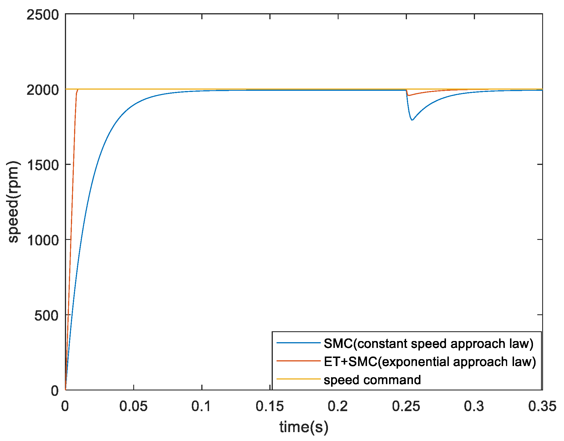
Figure 7.
Comparison of speed control responses between the proposed robust controller and the SMC using constant speed approach law (speed command increases to after 0.15 seconds, and at 0.25 seconds, load changes from N-m).
Figure 7.
Comparison of speed control responses between the proposed robust controller and the SMC using constant speed approach law (speed command increases to after 0.15 seconds, and at 0.25 seconds, load changes from N-m).
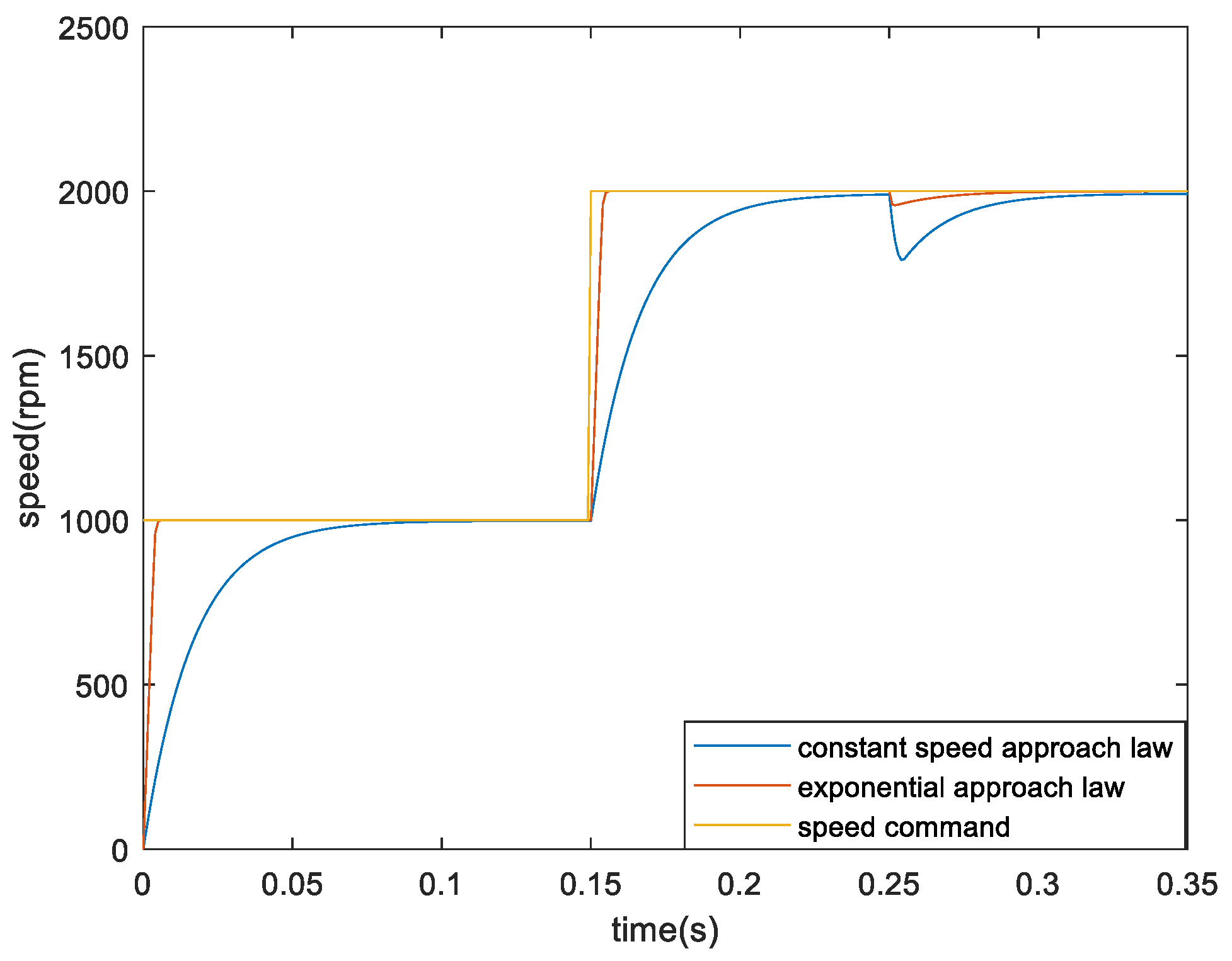
Figure 8.
Comparison of speed control responses between the proposed robust controller and the SMC using constant speed approach law (speed command decreases to after 0.15 seconds, and at 0.25 seconds, load changes from N-m).
Figure 8.
Comparison of speed control responses between the proposed robust controller and the SMC using constant speed approach law (speed command decreases to after 0.15 seconds, and at 0.25 seconds, load changes from N-m).

Figure 9.
Comparison of speed control response between the proposed robust controller and the SMC employing the constant speed approach law (speed command with load change from N-m at 0.15 seconds, and at 0.25 seconds, load change from N-m).
Figure 9.
Comparison of speed control response between the proposed robust controller and the SMC employing the constant speed approach law (speed command with load change from N-m at 0.15 seconds, and at 0.25 seconds, load change from N-m).
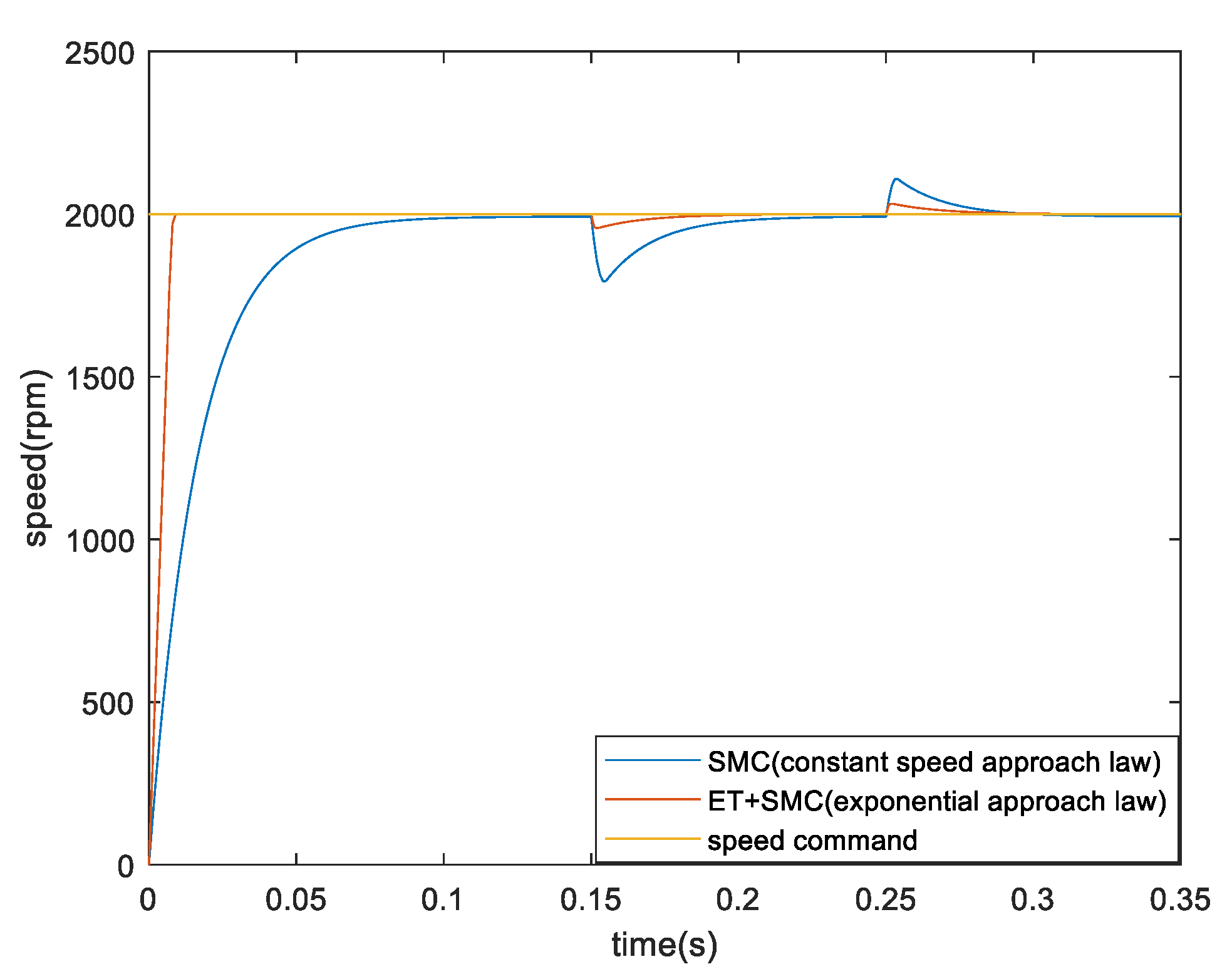
From the simulation results in Figures 6 to 9, it is observed that the robust controller proposed in this paper, which combines ET with SMC using exponential approach law, exhibits better dynamic response and steady-state response in tracking speed commands compared to the SMC with constant speed approach law. Additionally, under load variations, the speed recovery response of the proposed robust controller not only has a smaller recovery amplitude but also a shorter recovery time, and it reaches a steady state. Therefore, compared to the traditional SMC using constant speed approach law, the robust controller proposed in this paper achieves better speed control response due to its self-adaptive capability.
5. Conclusion
This paper combines ET with the exponential approach law of a SMC, replacing the traditional P-I speed controller used in FOC for BLDCM speed control. The proposed robust controller determines the control gain of the SMC by integrating ET, thereby adjusting the parameters of the sliding surface function. This approach suppresses the overshoot caused by the SMC using only exponential approach law, while also addressing the issue of slower response speed in traditional SMCs. Therefore, it improves performance in speed command tracking and load regulation response. Additionally, the proposed control method does not require extensive computation or learning data, making it easy to implement.
Author Contributions
K.-H.C. manages the project and completed the formal analysis of the extension controller. K.-H.C. also plans the project and writes, edits and reviews the manuscript. C.-T.H. ompleted the formal analysis of the sliding mode controller. X.-J.C. is responsible for the software program and simulation results validation. All authors have read and agreed to the published version of the manuscript.
Funding
The authors gratefully acknowledge the support and funding of this project by Industrial Technology Research Institute, Taiwan, under the Grant Number NCUT23TCE09 and NCUT23TCE021.
Institutional Review Board Statement
Not applicable.
Informed Consent Statement
Not applicable.
Data Availability Statement
This study did not report any data.
Conflicts of Interest
The authors of the manuscript declare no conflicts of interest.
References
- Wang, M.; Chen, Z. Research on Permanent Magnet Structure of Permanent Magnet Synchronous Motor for Electric Vehicle. In Proceedings of the 2nd International Conference on Electrical Engineering and Control Science (IC2ECS), Nanjing, China, 16–18 December 2022; pp. 990–993. [Google Scholar] [CrossRef]
- Lee, C. I.; Jang, G. H. Experimental Measurement and Simulated Verification of the Unbalanced Magnetic Force in Brushless DC Motors. IEEE Trans. Magnetics 2008, 44, 4377–4380. [Google Scholar] [CrossRef]
- BV, P.; Balamurugan, A.; Selvathai, T.; Reginald, R.; Varadhan, J. Evaluation of different Vector Control methds for Electric Vehicle Application. In Proceedings of the 2nd International Conference on Power and Embedded Drive Control (ICPEDC), Chennai, India, 21–23 August 2019; pp. 273–278. [Google Scholar] [CrossRef]
- Bhatti, S. A.; Malik, S. A.; Daraz, A. Comparison of P-I and I-P controller by using Ziegler-Nichols tuning method for speed control of DC motor. In Proceedings of the International Conference on Intelligent Systems Engineering (ICISE), Islamabad, Pakistan, 15–17 January 2016; pp. 330–334. [Google Scholar] [CrossRef]
- Murali, S. B.; Rao, P. M. Adaptive sliding mode control of BLDC motor using cuckoo search algorithm. In Proceedings of the 2nd International Conference on Inventive Systems and Control (ICISC), Coimbatore, India, 19-20 January 2018; pp. 989–993. [Google Scholar] [CrossRef]
- Chao, K.-H.; Chang, L.-Y.; Hung, C.-Y. Design and Control of Brushless DC Motor Drives for Refrigerated Cabinets. Energies 2022, 15, 3453. [Google Scholar] [CrossRef]
- Khanke, P. K.; Jain, S. D. Comparative analysis of speed control of BLDC motor using PI, simple FLC and Fuzzy - PI controller. In Proceedings of the International Conference on Energy Systems and Applications, Pune, India, 30 October–01 November 2015; pp. 296–301. [Google Scholar] [CrossRef]
- Longfei, J.; Yuping, H.; Jigui, Z.; Jing, C.; Yunfei, T.; Pengfei, L. Fuzzy Sliding Mode Control of Permanent Magnet Synchronous Motor Based on the Integral Sliding Mode Surface. In Proceedings of the 22nd International Conference on Electrical Machines and Systems (ICEMS), Harbin, China, 11–14 August 2019; pp. 1–6. [Google Scholar] [CrossRef]
- Qi, C.; Xie, J.; Mao, H.; Xie, Q. Condition Assessment of Valve-side Bushing of Converter Transformer Based on Extension Theory. In Proceedings of the IEEE International Conference on High Voltage Engineering and Application (ICHVE), Beijing, China, 06–10 September 2020; pp. 1–4. [Google Scholar] [CrossRef]
- Wang, J.; Ye, J.; Yan, R. The Magnetostatic Simulation and Determination of Magnetic Components for an External Ventricular Drainage Device. In Proceedings of the 40th Chinese Control Conference (CCC), Shanghai, China, 26–28 July 2021; pp. 6386–6391. [Google Scholar] [CrossRef]
- Kishore, N.; Shukla, K.; Gupta, N. A Novel Three-Phase Multilevel Inverter Cascaded by Three-Phase Two-Level Inverter and Two Single-Phase Boosted H-Bridge Inverters. In Proceedings of the IEEE PES Innovative Smart Grid Technologies - Asia (ISGT Asia), Singapore, Singapore, 01–05 November 2022; pp. 330–334. [Google Scholar] [CrossRef]
- Xie, T.; Kuai, Z.; Ye, X.; Zhu, L.; Guo, K.; Shi, S. Coordinate Conversions and Deviation Analysis in Multi-source Data Fusion. In Proceedings of the 2nd China International SAR Symposium (CISS), Shanghai, China, 03–05 November 2021; pp. 1–3. [Google Scholar] [CrossRef]
- Yadunandan; Naik, B.; Konduru, R.; Ilkal, B. B.; Kalligudd, S. Terminal Voltage control of BLDC Motor. In Proceedings of the International Conference on Smart Systems for applications in Electrical Sciences (ICSSES), Tumakuru, India, 07–08 July 2023; pp. 1–5. [CrossRef]
- Wu, H.-Q.; Chen, Y.-W.; Liu, R. College Education Outcome Expectation and Proactive Personality as Predictors of Chinese College Students’ Learning Motivation, Career Adaptability as a Mediator. In Proceedings of the International Conference on Modern Education and Information Management (ICMEIM), Dalian, China, 25–27 September 2020; pp. 716–721. [Google Scholar] [CrossRef]
- Zhang, L.; Li, Z.; Ma, H.; Ju, P. Power transformer fault diagnosis based on extension theory. In Proceedings of the International Conference on Electrical Machines and Systems, Nanjing, China, 27–29 September 2005; pp. 1763–1766. [Google Scholar] [CrossRef]
- Luo, N.; Zhang, L. Chaos Driven Development for Software Robustness Enhancement. In Proceedings of the 9th International Conference on Dependable Systems and Their Applications (DSA), Wulumuqi, China, 04–05 August 2022; pp. 1029–1034. [Google Scholar] [CrossRef]
- Guo, X.; Huang, S.; Peng, Y. Sliding Mode Speed Control of PMSM Based on A Novel Hybrid Reaching Law and High-Order Terminal Sliding-Mode Observer. In Proceedings of the IEEE 4th International Electrical and Energy Conference (CIEEC), Wuhan, China, 28–30 May 2021; pp. 1–6. [Google Scholar] [CrossRef]
- Zhang, J.; Liu, B.; Jiang, Z.; Hu, H. The Application of Sliding Mode Control with Improved Approaching Law in Manipulator Control. In Proceedings of the 13th IEEE Conference on Industrial Electronics and Applications (ICIEA), Wuhan, China, 31 May–02 June 2018; pp. 807–812. [Google Scholar] [CrossRef]
- Bodur, F.; Kaplan, O. A Novel Sliding Mode Control Based on Super Twisting Reaching Law for PMSM Speed Controller with Fixed-Time Disturbance Observer. In Proceedings of the 12th International Conference on Renewable Energy Research and Applications (ICRERA), Oshawa, ON, Canada, 29 August–01 September 2023; pp. 1–6. [Google Scholar] [CrossRef]
- Zeng, X.; Zeng, X.; Hong, Y. Distributed Computation of Common Lyapunov Functions. In Proceedings of the 37th Chinese Control Conference (CCC), Wuhan, China, 25–27 July 2018; pp. 2418–2423. [Google Scholar] [CrossRef]
- Wang, Q.; Chen, J.; Zhou, Z. Simulation of Sliding Mode Control for PMSM on Account of Variable Exponential Approach Law. In Proceedings of the Chinese Automation Congress (CAC), Hangzhou, China, 22–24 November 2019; pp. 3518–3521. [Google Scholar] [CrossRef]
Figure 1.
Equivalent circuit of a three-phase BLDCM in a stationary frame.
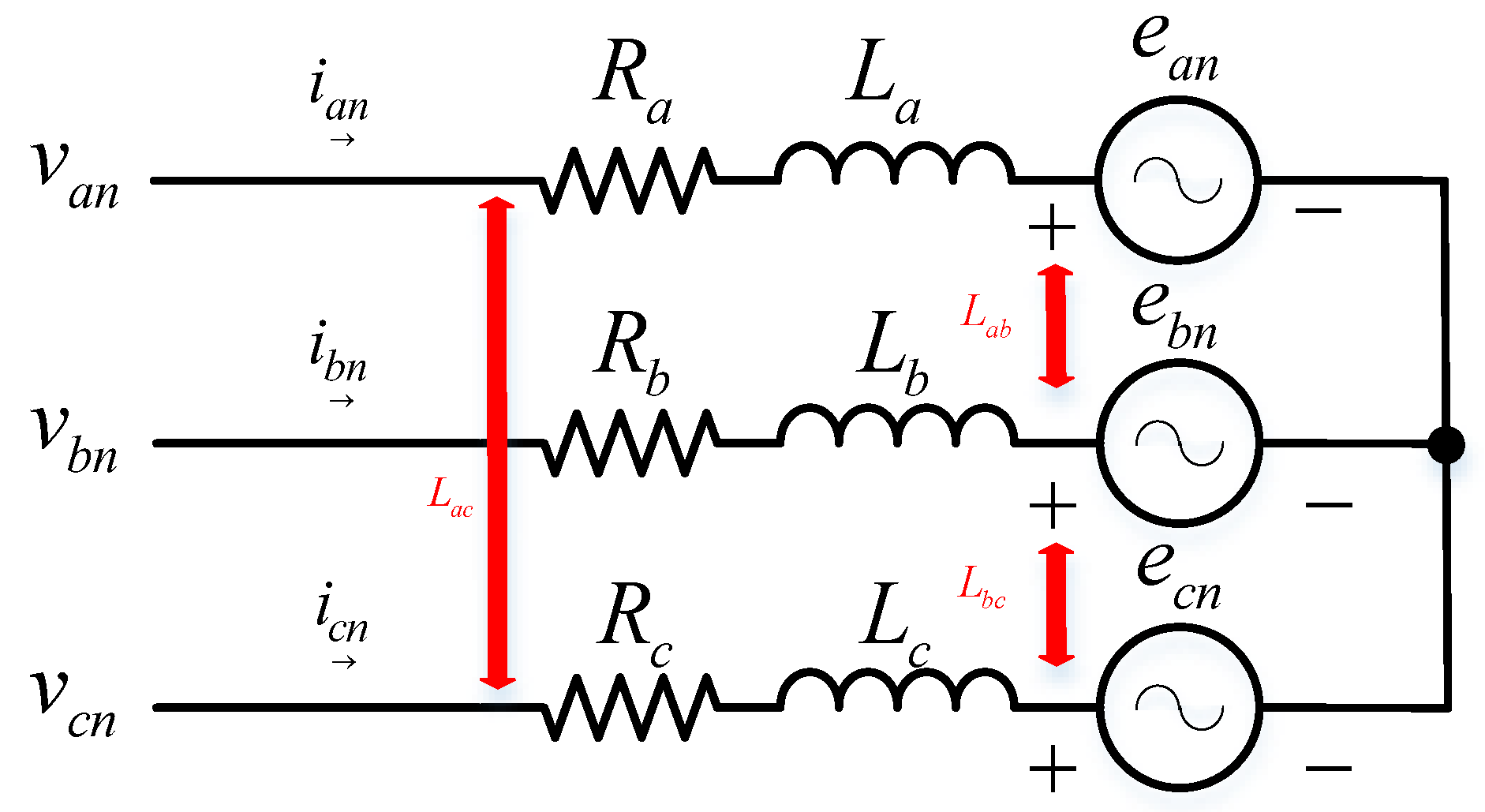
Figure 2.
FOC block diagram for the BLDCM.
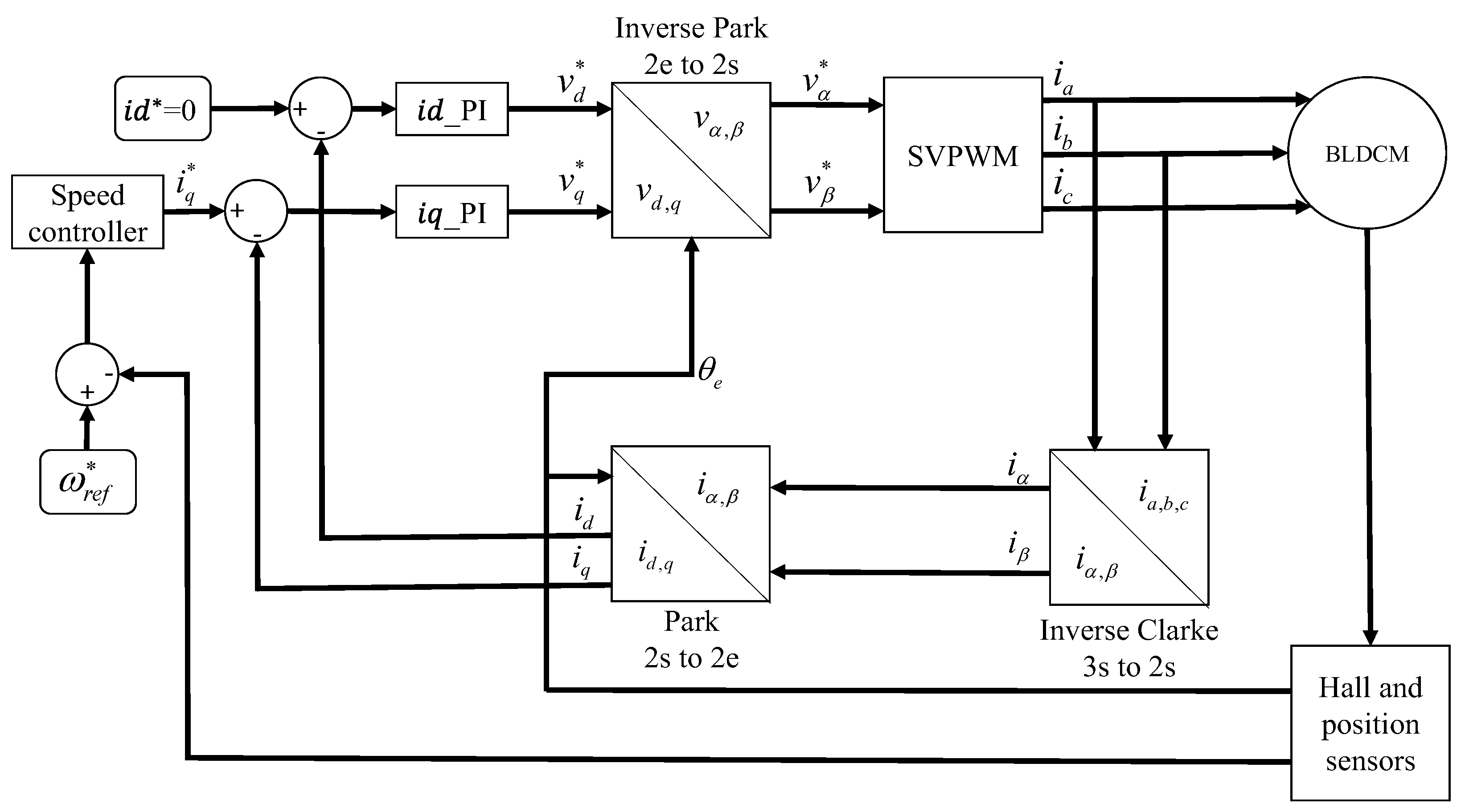
Figure 3.
Schematic diagram of the elementary correlation function.
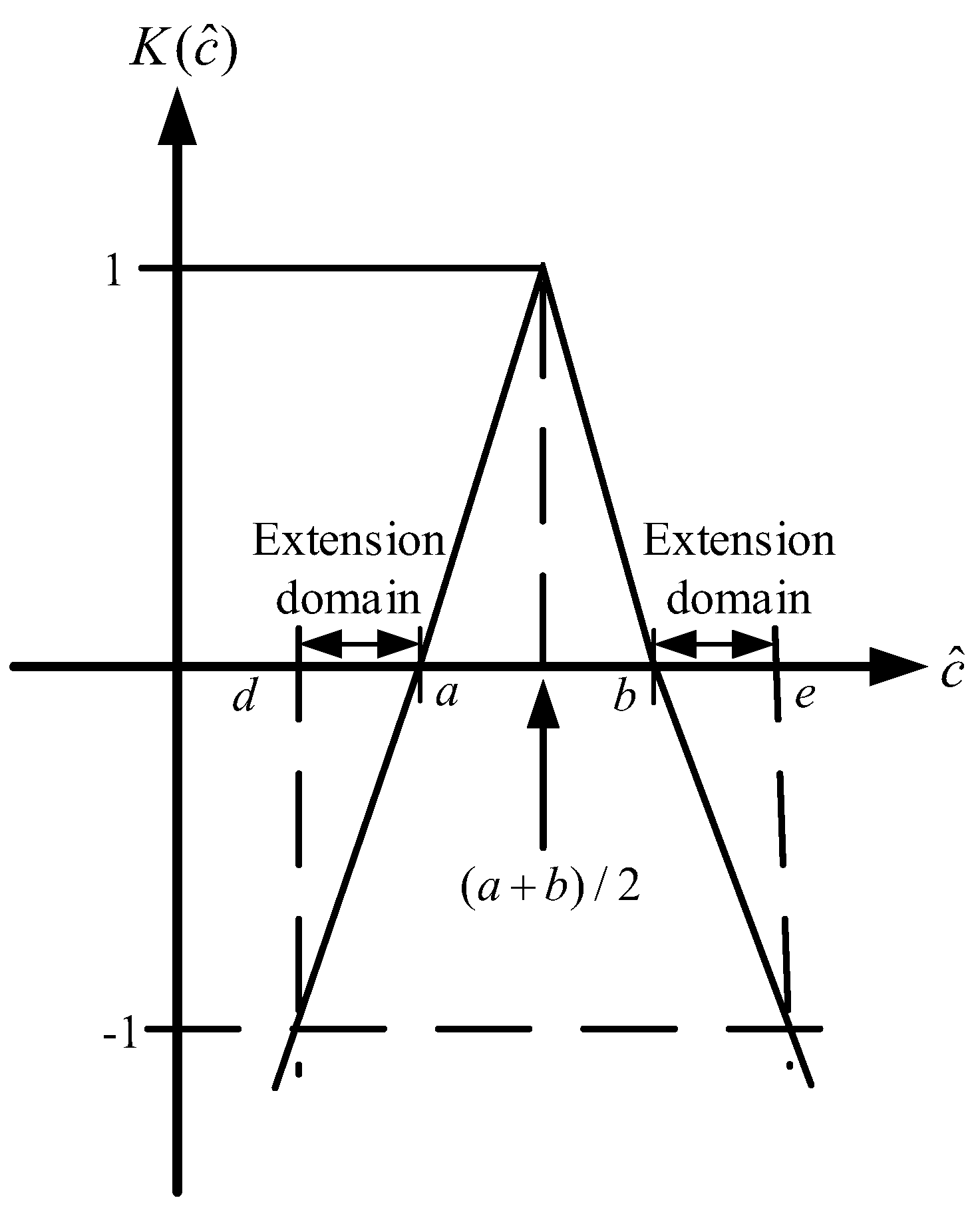
Figure 4.
Dynamic analysis chart of speed difference and variance rate of speed difference for BLDCM.
Figure 4.
Dynamic analysis chart of speed difference and variance rate of speed difference for BLDCM.
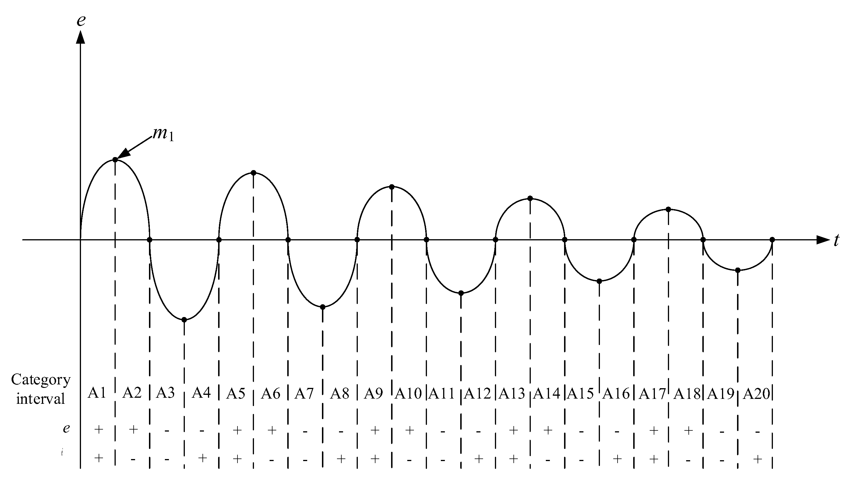
Figure 5.
Comparison of the speed response between the proposed robust controller and the sliding mode controller using only the exponential approach law.
Figure 5.
Comparison of the speed response between the proposed robust controller and the sliding mode controller using only the exponential approach law.
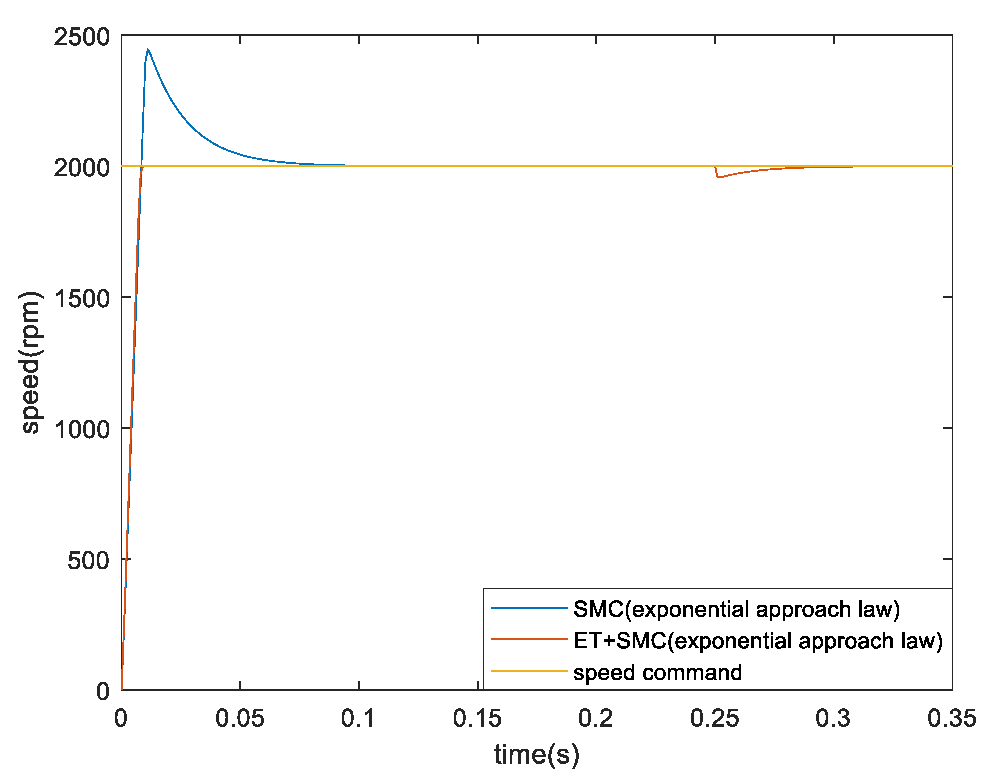

Table 1.
Extension matter element models and variation in control gain for 20 intervals of SMC.
| Interval | Extension matter element model | Variation of control gain |
| A1 | 0 | |
| A2 | 0 | |
| A3 | 0 | |
| A4 | 0 | |
| A5 | 15 | |
| A6 | 15 | |
| A7 | 15 | |
| A8 | 15 | |
| A9 | 30 | |
| A10 | 30 | |
| A11 | 30 | |
| A12 | 30 | |
| A13 | 45 | |
| A14 | 45 | |
| A15 | 45 | |
| A16 | 45 | |
| A17 | 60 | |
| A18 | 60 | |
| A19 | 60 | |
| A20 | 60 |
Disclaimer/Publisher’s Note: The statements, opinions and data contained in all publications are solely those of the individual author(s) and contributor(s) and not of MDPI and/or the editor(s). MDPI and/or the editor(s) disclaim responsibility for any injury to people or property resulting from any ideas, methods, instructions or products referred to in the content. |
© 2024 by the authors. Licensee MDPI, Basel, Switzerland. This article is an open access article distributed under the terms and conditions of the Creative Commons Attribution (CC BY) license (http://creativecommons.org/licenses/by/4.0/).
Copyright: This open access article is published under a Creative Commons CC BY 4.0 license, which permit the free download, distribution, and reuse, provided that the author and preprint are cited in any reuse.