Location Problem in Relativistic Positioning: Relative Formulation

A relativistic positioning system is a set of four emitters broadcasting their proper times by means of light signals. The four emitter times received at an event constitute the emission coordinates of the event. Covariant quantities associated with relativistic positioning systems are analysed relatively to an observer in Minkowski space-time by splitting them in their relative space-like and time-like components. The location of a user in inertial coordinates from a standard set of emission data (emitted times and satellite trajectories) is solved in the underlying 3+1 formalism. The analytical location solution obtained by Kleusberg for the GPS system is recovered and interpreted in a Minkowskian context.

Keywords:

Subject: Physical Sciences - Other

1. Introduction

The central question in positioning theories is to determine the location of the user without ambiguity after solving the navigation equations.

For users of Global Navigation Satellite Systems (GNSS), such as GPS and Galileo, these navigation equations are usually formulated in terms of pseudoranges, which are the apparent distances to the user from each of the emitters as inferred from the travel time of the signal (see Section 4 for more detail).

In general, the procedures used in GNSS to solve the equations analytically can be divided in two classes, depending on whether they use pseudoranges (Bancroft’s algorithm, [1]) or pseudorange differences (Kleusberg’s method, [2,3]), thus eliminating the user clock bias (see Section 4). In line with [1], Abel and Chaffee stated the problem using the Lorentz scalar product [4] and analyzed the existence and non-unicity of the solutions [5] (bifurcation), which was also considered in [6].

A fully relativistic formulation of the problem in Minkowski space-time was given in the context of the theory of Relativistic Positioning Systems (RPS) [7,8]. For the foundations, genesis, objectives and perspectives of the RPS theory, refer to [9,10,11,12] and references therein. Recently, Bancroft’s solution [1] was interpreted in the language of RPS [13,14], but the corresponding RPS interpretation of Kleusberg’s solution remained to be done. This complementary task is achieved in this paper.

Recall that a RPS is a set of four ordered clocks A

(A = 1, 2, 3, 4)

, of world-lines

γ_{A} (τ^{A})

, broadcasting their times

τ^{A}

by means of light signals. For simplicity, and as it will be the case in the present work, the time considered is the proper time. The four times

{τ^{A}}

received by an event x constitute the emission coordinates of the event [15]. Again for simplicity, the emission and reception processes are assumed continuous. For the theory and classification of RPS based on a discrete set of data, see [16].

Current GNSS do not broadcast the proper time of their clocks, but the system’s own time (the GPS or the Galileo time), a time which, roughly speaking, coincides up to a fixed shift with the International Atomic Time.

In any case, for every set of four satellites in a given constellation (that could include both GPS and Galileo satellites) the four broadcast times essentially share the algebraic and differential properties characterizing an emission coordinate system. These properties have been analyzed elsewhere [7,15], and they do not need to be exhaustively remembered here. Only a property needs to be highlighted now, that concerns the very unusual character of the emission coordinates: all the gradients

d τ^{A}

are light-like. This means that

{τ^{A}}

is a set of four null gradient coordinates, an outstanding property that wholly determines the causal class of every relativistic emission coordinate system [17].

Suppose there is a specific coordinate system

{x^{α}}

covering the whole region of emission coordinates, let

γ_{A} (τ^{A})

be the world-lines of the clocks A with respect to this particular coordinate system and let

{τ^{A}}

be the values of the emission coordinates received by a user. The data set

E \equiv

{γ_{A} (τ^{A}), {τ^{A}}}

is called the standard data set.

The location problem with respect to E, also called the standard location problem or the E-location problem for short, is the problem of finding the coordinates

{x^{α}}

of the user from the sole data E, by solving the following algebraic system of four non-linear equations (called the null propagation equations):

{(x - γ_{A})}^{2} = 0, A = 1, 2, 3, 4 .

(1)

The covariant solution to the standard location problem in Minkowski space-time has been already discussed [7,8]. Nevertheless, it remains to be formulated in the framework of an arbitrary inertial coordinate system associated with an inertial observer u (

u^{2} = - 1

), that is, by describing space-time from its relative splitting in space plus time with respect to u. Then, the unknown space-time position x of the user can be split, relatively to u, in inertial components

{x^{0}, \vec{x}}

as:

x = x^{0} u + \vec{x}, x^{0} = - x \cdot u, \vec{x} \cdot u = 0 .

(2)

From now on, we will take the speed of light in vacuum

c = 1

and

t \equiv x^{0}

(see Appendix 7 for the notation used in this article).

The matter is then how to determine, with respect to u, the solution of the standard location problem, that is, the coordinate transformation from emission to inertial coordinates,

x^{0} (τ^{A})

and

\vec{x} (τ^{A})

, when the motions of the emitters are known (received data) in the inertial coordinate system. For this purpose, the tensor quantities that are intrinsically related to the configuration of the emitters at x have to be split in time-like and space-like components. Once the splitting is accomplished, we can recover Kleusberg’s analytical solution [3] used in GPS navigation [18].

The covariant solution [7,8] has been used in the construction of numerical algorithms for positioning in flat and curved space-times [19,20,21,22]. The statement of the location problem in exact Schwarzschild metric and its perturbative treatment has been modelled in [23,24,25].

The paper is organized as follows. In Section 2, the geometric objects (vector and bivectors) associated with the configuration of the emitters for the reception event are decomposed in time-like and space-like components, relatively to an inertial observer. Section 3 is devoted to split, relatively to an inertial observer, the covariant formula giving the location of a user in relativistic positioning. In Section 4 we use the preceding splittings to express Kleusberg’s procedure in a relativistic formalism and to recover Kleusberg’s solution from the covariant solution. In Section 5 an alternative expression of the covariant solution in terms of the principal directions of the configuration bivector is provided. The principal directions are split relatively to an inertial observer and Kleusberg’s solution is again recovered. The results are summarized and discussed in Section 6. Appendix 7 is devoted to summarise the notation and conventions used.

Some preliminary results of this work were communicated without proof at the ESA-Advanced Concepts Team Workshop “Relativistic Positioning Systems and their Scientific Applications” (see Ref. [26]).

2. Configuration of the Emitters Underlying Geometry

In relativistic positioning terminology, the configuration of the emitters for an event P is the set of four events

{γ_{A} (τ^{A})}

of the emitters at the emission times

{τ^{A}}

received at P. The covariant solution [7] to the standard location problem depends on the configuration of the emitters through different scalars, vectors and bivectors, all of which computable from the standard data set

{γ_{A} (τ^{A}), {τ^{A}}}

. These quantities are analyzed in this section.

The set

R

of events which are reached by the broadcast signals will be called the emission region of the RPS. Then, if

P \in R

, let us denote by

x \equiv O P

the position vector with respect the origin O of a given inertial system. If a user at P receives the broadcast times

{τ^{A}}

γ_{A}

denote the position vectors of the emitters at the emission times,

γ_{A} \equiv O γ_{A} (τ^{A})

. The trajectories followed by the light signals from the emitters

γ_{A} (τ^{A})

to the reception event P are described by the vectors

m_{A} \equiv x - γ_{A}

. Let us choose a reference emitter (say

A = 4

) and refer to it the other emitters (referred emitters). Then, the position vector of the a-th emitter with respect to the reference emitter is written as (see Figure 1a)

\begin{matrix} e_{a} = γ_{a} - γ_{4} = m_{4} - m_{a} (a = 1, 2, 3) . \end{matrix}

(3)

The world function [27,28] of the end point of

e_{a}

is the scalar

Ω_{a} = \frac{1}{2} {(e_{a})}^{2} .

(4)

As discussed in [7], the emission/reception conditions imply

Ω_{a} > 0

2.1. Splitting of $γ_{A}$ , $m_{A}$ and $e_{a}$

The position vectors

γ_{A}

can be decomposed, relatively to u, as:

γ_{A} = t_{A} u + {\vec{γ}}_{A} (A = 1, 2, 3, 4),

(5)

where

t_{A} \equiv γ_{A}^{0}

is the coordinate inertial time of the event

γ_{A} (τ^{A})

as measured by the inertial observer u. The vectors

m_{A}

are decomposed as follows:

\begin{matrix} m_{A} = (t - t_{A}) u + \vec{x} - {\vec{γ}}_{A} = m_{A}^{0} u + {\vec{m}}_{A} (A = 1, 2, 3, 4), \end{matrix}

(6)

being null and future pointing,

{(t - t_{A})}^{2} = {(\vec{x} - {\vec{γ}}_{A})}^{2}, t > t_{A} .

(7)

For later convenience we define

\begin{matrix} y \equiv x - γ_{4} = m_{4} = y^{0} u + \vec{y} . \end{matrix}

(8)

The position vector

e_{a}

of the a-th emitter with respect to the reference emitter is decomposed as (see Figure 1b)

\begin{matrix} e_{a} = σ_{a} u + {\vec{e}}_{a}, σ_{a} = t_{a} - t_{4}, {\vec{e}}_{a} = {\vec{γ}}_{a} - {\vec{γ}}_{4} (a = 1, 2, 3) . \end{matrix}

(9)

With the inertial components of

e_{a}

{σ_{a}, {\vec{e}}_{a}}

, we can express the world function (4) as:

Ω_{a} = \frac{1}{2} ({({\vec{e}}_{a})}^{2} - σ_{a}^{2}) = \frac{1}{2} [{({\vec{γ}}_{a} - {\vec{γ}}_{4})}^{2} - {(t_{a} - t_{4})}^{2}] .

(10)

2.2. Splitting of the Configuration Vector $χ$

Here we always consider that, for the reception event P, the emitter configuration is regular, that is, the four emission events

{γ_{A} (τ^{A})}

determine a hyperplane named the configuration hyperplane for P. Or equivalently, we assume that the configuration vector

χ

, defined as:

χ \equiv * (e_{1} \land e_{2} \land e_{3})

(11)

is nonzero,

χ \neq 0

. The star * stands for the Hodge dual operator associated with the metric volume element

η = (η_{α β μ ν})

. One has

χ_{α} = η_{α β μ ν} e_{1}^{β} e_{2}^{μ} e_{3}^{ν} \neq 0

. Non-regular emitter configurations (with

χ = 0

) can sporadically occur in current global navigation systems as it was stressed and considered in [4,5].

Substituting (3) in (11) and taking into account (108) and (109) we have

\begin{matrix} χ & = σ_{1} * (u \land {\vec{e}}_{2} \land {\vec{e}}_{3}) + σ_{2} * ({\vec{e}}_{1} \land u \land {\vec{e}}_{3}) + σ_{3} * ({\vec{e}}_{1} \land {\vec{e}}_{2} \land u) + * ({\vec{e}}_{1} \land {\vec{e}}_{2} \land {\vec{e}}_{3}) \\ = ({\vec{e}}_{1}, {\vec{e}}_{2}, {\vec{e}}_{3}) u + σ_{1} {\vec{e}}_{2} \times {\vec{e}}_{3} + σ_{2} {\vec{e}}_{3} \times {\vec{e}}_{1} + σ_{3} {\vec{e}}_{1} \times {\vec{e}}_{2}, \end{matrix}

where × denotes the cross product between vectors in the 3-space orthogonal to u,

E_{⊥}

(see Appendix 7). The following result concerning the decomposition of

χ

in time-like and space-like components holds.

Proposition 1.

Relatively to an inertial observer u, the configuration vector is expressed as

χ = χ^{0} u + \vec{χ}

, with

χ^{0} = ({\vec{e}}_{1}, {\vec{e}}_{2}, {\vec{e}}_{3}), \vec{χ} = \frac{1}{2} ϵ^{a b c} σ_{a} {\vec{e}}_{b} \times {\vec{e}}_{c},

(12)

where

{σ_{a}, {\vec{e}}_{a}}

are the components of the position vectors of the referred emitters.

Then, we see that

| χ^{0} |

is the volume of the parallelepiped defined by the relative positions

{\vec{e}}_{a}

of the referred emitters. On the other hand,

\vec{χ}

represents a weighted vector-area. The area

A_{b c}

of the face generated by

{\vec{e}}_{b}

and

{\vec{e}}_{c}

is weighted with a complementary

σ_{a}

factor. Then

| σ_{a} {\vec{e}}_{b} \times {\vec{e}}_{c} | = c | t_{c} - t_{4} | A_{b c}

(13)

is the volume of the time-like parallelepiped generated by

{σ_{a} u, {\vec{e}}_{b}, {\vec{e}}_{c}}

2.3. Splitting of the Bivectors $E^{a}$

The positions of the referred emitters,

e_{a}

, generate the bivectors

E^{a}

which are defined as

E^{1} = * (e_{2} \land e_{3}), E^{2} = * (e_{3} \land e_{1}), E^{3} = * (e_{1} \land e_{2}),

(14)

that is,

E^{a} = * (e_{a + 1} \land e_{a + 2})

, where the notation is understood modulo 3. By using index notation, one can write, for example,

\begin{matrix} {(e_{a} \land e_{b})}^{μ ν} = e_{a}^{μ} e_{b}^{ν} - e_{b}^{μ} e_{a}^{ν}, \end{matrix}

(15)

\begin{matrix} {[* (e_{a} \land e_{b})]}_{α β} = \frac{1}{2} η_{α β μ ν} {(e_{a} \land e_{b})}^{μ ν} = η_{α β μ ν} e_{a}^{μ} e_{b}^{ν} . \end{matrix}

(16)

Then, according to (108), one obtains

i (u) * (e_{a} \land e_{b}) = - {\vec{e}}_{a} \times {\vec{e}}_{b}

(17)

with

i ()

the interior product (defined in Appendix 7) and where we have taken into account (9).

For an observer u, the electric and magnetic parts of a bivector

E^{a}

are vectors in the 3-space orthogonal to u, which are defined as

{\vec{S}}^{a} = - i (u) E^{a}, {\vec{B}}^{a} = - i (u) * E^{a},

(18)

respectively. Then, from (17) and taking into account the identity

* (* E^{a}) = - E^{a}

and (9), we have

\begin{matrix} {\vec{S}}^{a} & = - i (u) * (e_{a + 1} \land e_{a + 2}) = {\vec{e}}_{a + 1} \times {\vec{e}}_{a + 2}, \end{matrix}

(19)

\begin{matrix} {\vec{B}}^{a} & = i (u) (e_{a + 1} \land e_{a + 2}) = - σ_{a + 1} {\vec{e}}_{a + 2} + σ_{a + 2} {\vec{e}}_{a + 1}, \end{matrix}

(20)

where these equalities are understood modulo 3.

Thus, the following result is established.

Proposition 2.

Relatively to an inertial observer u, the configuration 2-forms are expressed as

\begin{matrix} E^{a} = u \land {\vec{S}}^{a} - * (u \land {\vec{B}}^{a}), \end{matrix}

(21)

\begin{matrix} {\vec{S}}^{a} \equiv {\vec{e}}_{a + 1} \times {\vec{e}}_{a + 2}, {\vec{B}}^{a} \equiv ϵ^{a b c} σ_{c} {\vec{e}}_{b}, \end{matrix}

(22)

where

{σ_{a}, {\vec{e}}_{a}}

are the components of the position vectors of the referred emitters.

2.4. Splitting of the Configuration Bivector H

For each emitter

γ_{A}

we can define a configuration bivector

H_{(A)}

with respect to that emitter. In the present work, we will define

H \equiv H_{(4)}

as the configuration bivector with respect to the reference emitter

γ_{4}

H = Ω_{a} E^{a} = Ω_{1} E^{1} + Ω_{2} E^{2} + Ω_{3} E^{3} .

(23)

Relatively to an inertial observer u, this bivector can be written as

H = u \land \vec{S} - * (u \land \vec{B}),

(24)

where

\vec{S} = - i (u) H

and

\vec{B} = - i (u) * H

are, respectively, the electric and magnetic parts of H relative to u. Taking into account (21)-(23),

\vec{S}

and

\vec{B}

are given according to the following:

Proposition 3.

Relatively to an inertial observer u, the electric and magnetic parts,

\vec{S}

and

\vec{B}

, into which the configuration bivector H is split, can be expressed as:

\begin{matrix} \vec{S} & = Ω_{a} {\vec{S}}^{a} = Ω_{1} ({\vec{e}}_{2} \times {\vec{e}}_{3}) + Ω_{2} ({\vec{e}}_{3} \times {\vec{e}}_{1}) + Ω_{3} ({\vec{e}}_{1} \times {\vec{e}}_{2}), \end{matrix}

(25)

\begin{matrix} \vec{B} & = Ω_{a} {\vec{B}}^{a} = (Ω_{3} σ_{2} - Ω_{2} σ_{3}) {\vec{e}}_{1} + (Ω_{1} σ_{3} - Ω_{3} σ_{1}) {\vec{e}}_{2} + (Ω_{2} σ_{1} - Ω_{1} σ_{2}) {\vec{e}}_{3} . \end{matrix}

(26)

As was noted in [8], since the invariant

H_{μ ν} {(* H)}^{μ ν}

identically vanishes, it always occurs that

\vec{S} \cdot \vec{B} = 0

, which also results from (25) and (26).

We can now express the splitting of the configuration vector

χ

(12) in terms of

\vec{S}

and

\vec{B}

, which follows from (25) and (26) by the scalar and cross product with

{\vec{e}}_{a}

Proposition 4.

Relatively to an inertial observer u, the configuration vector is expressed as

χ = χ^{0} u + \vec{χ}

, with

\begin{matrix} χ^{0} = \frac{\vec{S} \cdot {\vec{e}}_{a}}{Ω_{a}}, \vec{χ} = \frac{σ_{a} \vec{S} + {\vec{e}}_{a} \times \vec{B}}{Ω_{a}}, \end{matrix}

(27)

for any

a = 1, 2, 3

, where

{σ_{a}, {\vec{e}}_{a}}

are the components of the position vectors of the referred emitters.

3. The Location Problem

The E-location problem in flat space-time has been analyzed in [7,8], especifically considering an inertial coordinate system

{x^{α}}

. The result may be expressed in a closed formula that we explain below. The goal of this section is to separate this formula in time-like and space-like components by splitting, relatively to an inertial observer, the quantities involved in the covariant solution to the E-location problem.

The transformation from emission to inertial coordinates is expressed in closed form according to the following proposition (see [7,8]):

Proposition 5.

Let

γ_{A} (τ^{A})

be the world-lines of four arbitrary emitters of a RPS with respect to an inertial coordinate system

{x^{α}}

, and let

{τ^{A}}

be their emission coordinates. The coordinate transformation

x = K (τ^{A})

between emission and inertial coordinates is given by

\begin{matrix} x = γ_{4} + y_{*} + λ χ, \end{matrix}

(28)

\begin{matrix} y_{*} = \frac{1}{ξ \cdot χ} i (ξ) H, λ = - \frac{y_{*}^{2}}{(y_{*} \cdot χ) + \hat{ϵ} \sqrt{Δ}}, Δ = {(y_{*} \cdot χ)}^{2} - y_{*}^{2} χ^{2}, \end{matrix}

(29)

where ξ is any vector satisfying the transversality condition

ξ \cdot χ \neq 0

\hat{ϵ}

the orientation of the positioning system at x, which is given by

\hat{ϵ} = sgn [* (m_{1} \land m_{2} \land m_{3} \land m_{4})]

, χ the configuration vector and H the configuration bivector.

As set out in [7], the null propagation equations (1) can be expressed with respect to the reference emitter and be separated into a quadratic equation

\begin{matrix} y^{2} = 0, \end{matrix}

(30)

and a system of three linear equations

\begin{matrix} e_{a} \cdot y = Ω_{a}, a = 1, 2, 3 . \end{matrix}

(31)

The quantity

y_{*}

is the particular solution to the system (31). Note that

ξ \cdot y_{*} = 0

and that

y_{*}

is directly computable from the sole standard emission data, since

χ

and H are determined by the vectors

e_{a}

given by Eq. (3).

Further, the consistence of the above definition of

λ

is assured. Since the vectors

{y_{*}, χ}

and

{m_{4}, χ}

generate the same 2-plane, one has that

s g n (Δ) = s g n [{(χ \cdot m_{4})}^{2}]

, and then

Δ ⩾ 0

As was noticed in [8],

Δ

is the scalar invariant of H defined by

f \equiv \frac{1}{2} t r H^{2}

Δ = f = - \frac{1}{2} H_{μ ν} H^{μ ν},

(32)

and may be directly computed from H.

3.1. Splitting of the Particular Solution $y_{*}$

In this subsection, we carry out the relative decomposition of the particular solution

y_{*}

appearing in Eq. (28). From Eq. (29), the splitting of

y_{*}

is obtained by splitting the vector

i (ξ) H

. To begin with, notice that the transversal vector

ξ

can be always chosen so that its time-like component,

ξ^{0}

, is equal to one,

ξ^{0} = - ξ \cdot u = 1

, that is

ξ = u + \vec{ξ} .

(33)

Thus, the transversality condition says that

χ^{0} \neq \vec{ξ} \cdot \vec{χ}

and from Proposition 1 this other result follows.

Proposition 6.

Relatively to an inertial observer u, the transversality condition,

ξ \cdot χ \neq 0

, is expressed as

({\vec{e}}_{1}, {\vec{e}}_{2}, {\vec{e}}_{3}) \neq \frac{1}{2} ϵ^{a b c} σ_{a} (\vec{ξ}, {\vec{e}}_{b}, {\vec{e}}_{c}) .

(34)

Then, from (33) and (24), we have

\begin{matrix} i (ξ) H = - \vec{S} - (\vec{ξ} \cdot \vec{S}) u + * (ξ \land u \land \vec{B}) = - (\vec{ξ} \cdot \vec{S}) u - \vec{S} - \vec{ξ} \times \vec{B} \end{matrix}

and the following statement holds.

Proposition 7.

Relatively to an inertial observer u, the particular solution

y_{*}

orthogonal to

ξ = u + \vec{ξ}

is expressed as

y_{*} = y_{*}^{0} u + {\vec{y}}_{*},

(35)

where

y_{*}^{0} = - \frac{\vec{ξ} \cdot \vec{S}}{D}, {\vec{y}}_{*} = - \frac{\vec{S} + \vec{ξ} \times \vec{B}}{D},

(36)

with the transversality condition expressed as

D \equiv ξ \cdot χ = \vec{ξ} \cdot \vec{χ} - ({\vec{e}}_{1}, {\vec{e}}_{2}, {\vec{e}}_{3}) \neq 0 .

(37)

The vectors

\vec{χ}

\vec{S}

and

\vec{B}

are obtained from the positioning data using Eqs. (12), (25) and (26).

3.2. Splitting of the Covariant Solution x

Eq. (28) gives the solution x for the E-location problem provided that

y_{*}

and

\hat{ϵ}

are obtained from a standard set of data

E \equiv

{γ_{A} (τ^{A}), {τ^{A}}}

. Relatively to an inertial observer u, the solution x is split as

x = t u + \vec{x}

, with:

\begin{matrix} t = t_{4} + y_{*}^{0} + λ χ^{0}, \vec{x} = {\vec{γ}}_{4} + {\vec{y}}_{*} + λ \vec{χ} . \end{matrix}

(38)

In fact, according to Eq. (28), the determination of the scalar

λ

involves both

y_{*}

(given by (29)) and

\hat{ϵ}

. Propositions 1 and 3 provide, respectively, the inertial components of

χ

and H in terms of the data. Proposition 7 allows to determine

y_{*} = {y_{*}^{0}, {\vec{y}}_{*}}

. The invariant

Δ

can be computed from (24) and (32) to see that it has a clear geometric meaning according to the following:

Proposition 8.

Relatively to an inertial observer u, H splits in electric (

\vec{S}

) and magnetic (

\vec{B}

) parts, so that the invariant Δ is expressed as

Δ = {\vec{S}}^{2} - {\vec{B}}^{2} .

(39)

According to this proposition, the user knows when it is crossing the region where

Δ = 0

(44), namely, when

\vec{S}

and

\vec{B}

are equimodular. In this region, the user can still locate itself using Proposition 5.

Then, we can obtain

λ

λ = - \frac{- {(y_{*}^{0})}^{2} + {\vec{y}}_{*}^{2}}{(- y_{*}^{0} χ^{0} + {\vec{y}}_{*} \cdot \vec{χ}) + \hat{ϵ} \sqrt{{\vec{S}}^{2} - {\vec{B}}^{2}}} .

(40)

Notice that to make this expression for

λ

operative one needs to determine the orientation

\hat{ϵ}

, whose very definition (see Proposition 5) involves the unknown x. Therefore, the covariant solution of the standard location problem, given by (28), has to be accompanied with a method for obtaining

\hat{ϵ}

which does not involve the previous calculation of x.

This question was discussed in [7] showing that in the central region of the positioning system (the space-time region of all

x \in R

such that

χ^{2} \leq 0

, see Section 3.3 below) the orientation

\hat{ϵ}

is constant and can be obtained as

\hat{ϵ} = s g n (u \cdot χ)

for any future pointing time-like vector u. In particular, if u is an inertial observer,

\hat{ϵ} = - s g n (χ^{0}) = - s g n [({\vec{e}}_{1}, {\vec{e}}_{2}, {\vec{e}}_{3})] .

(41)

Note that from (12) and (27):

({\vec{e}}_{1}, {\vec{e}}_{2}, {\vec{e}}_{3}) = \frac{\vec{S} \cdot {\vec{e}}_{a}}{Ω_{a}}, for any a = 1, 2, 3,

(42)

and therefore, since

Ω_{a} > 0

\hat{ϵ} = - s g n (\vec{S} \cdot {\vec{e}}_{a}) .

(43)

Thus, we arrive at the following result.

Proposition 9.

On the central region of a RPS, the orientation

\hat{ϵ}

+ 1

- 1

\vec{S} \cdot {\vec{e}}_{a}

(a = 1, 2, 3)

is, respectively, negative or positive.

The determination of

\hat{ϵ}

from a set of observational data as well as its connection with the solution to the bifurcation problem (outside the central region) have been analyzed elsewhere [7,8], showing that the applicability of Proposition 5 has no strings attached. A brief account of the bifurcation problem follows.

3.3. Emission Coordinate Domains and Bifurcation Problem

Equation (28) is the coordinate transformation from emission to inertial coordinates,

x^{α} = K^{α} (τ^{A})

. The inverse transformation

Θ

, mapping to every x its emission coordinates,

τ^{A} = Θ^{A} (x)

, is known as the characteristic emission function. As shown in [8], if

j_{Θ} (x)

is the jacobian determinant of

Θ

j_{Θ} (x) = 0 iff Δ = 0 .

(44)

This property defines two different emission coordinate systems: the front emission coordinate system and the back emission coordinate system. As far as we remain in space-time regions where light signals do not bifurcate, the way emission coordinates are created by the relativistic positioning system imposes that the coordinate domains in space-time, of the front and of the back emission coordinate systems, are disjoint.

In addition, these coordinate domains are related by the following property: all of the values of the emission coordinates

{τ^{A}}

on the back emission coordinate domain are also values of the emission coordinates on a (generically proper) set of the front emission coordinate domain, which is called the time-like front region; the complementary set (in the front emission coordinate domain) of this time-like front region is called the central region of the relativistic positioning system [7,8].

This coincidence of values, of the emission coordinates in the back coordinate domain and in the time-like front coordinate domain, is at the origin of the bifurcation problem: how can the users of the relativistic positioning system know in which of the two coordinate domains of space-time they are? To answer this question the user needs to compute the causal character of the emitter configuration (at x): it is said to be space-like, light-like or time-like if

χ^{2} < 0

χ^{2} = 0

χ^{2} > 0

, respectively, at x. The regions defined by these conditions are respectively denoted as

C_{s}

C_{l}

and

C_{t}

. The central region is

C = C_{s} \cup C_{l}

. The time-like front region

C_{t}^{F}

and the central region form the front emission coordinate domain. The back emission coordinate domain is the time-like back region

C_{t}^{B}

Therefore, depending on the causal character of the configuration vector

χ

, we distinguish three situations (see Figures 3–5 in [8]):

If $χ$ is time-like, there is only one emission solution P, the other ( $P^{'}$ ) is a reception solution. In this case, the sign of $\hat{ϵ}$ can be determined from the sole standard emission data ${γ_{A} (τ^{A}), {τ^{A}}}$ (see Proposition 9).
If $χ$ is light-like, there is only one valid emission solution (the other solution is degenerate). The sign of $\hat{ϵ}$ can be determined from ${γ_{A} (τ^{A}), {τ^{A}}}$ (see Proposition 9).
If $χ$ is space-like, there are two valid emission solutions: in order to determine the sign of $\hat{ϵ}$ , additional observational information is necessary (relative positions of emitters on the user’s celestial sphere, see [8]).

4. Kleusberg’s Solution

In GNSS the pseudoranges are modelled considering the emitters’ positions at signal emission, user and emitter clock biases and different corrections affecting signal propagation [29,30]. The pseudorange equations are first linearized around an approximate position and then solved by iterative methods. The user’s approximate position is usually obtained using analytic (closed-form) solutions of the equations (neglecting emitter clock biases and signal propagation corrections), where the unknowns are the user’s coordinates and clock bias with respect to a certain reference frame and reference time. In this section we see how the relative formulation of the characteristic quantities of a RPS allows to interpret Kleusberg’s analytical solution to the GPS navigation equations [3].

4.1. Concepts and Notation

In [3] the starting point are the measured pseudoranges between the satellites and the user. The pseudoranges

p_{A}

are modelled as follows (taking the speed of light

c = 1

\begin{matrix} p_{A} = {[{(x - x_{A})}^{2} + {(y - y_{A})}^{2} + {(z - z_{A})}^{2}]}^{\frac{1}{2}} + d T, \end{matrix}

(45)

where

{x_{A}, y_{A}, z_{A}}

are the Cartesian coordinates of the A-th satellite (

A = 1, 2, 3, 4

) at the time

t_{A}

of emission,

{x, y, z}

those of the user at the time t of reception and

d T

the user’s clock

b i a s

, defined as the difference between the user’s clock time and the so-called GPS time.

Assuming that the bias

d T

is the same for all the satellites, it can be removed by subtracting one reference pseudorange (

p_{4}

) from the other three:

d_{a} : = p_{a} - p_{4}

a = 1, 2, 3

. In the covariant solution, this difference can be identified with

σ_{a} : = t_{a} - t_{4}

d_{a} ⟷ σ_{a} .

Kleusberg denotes the Euclidean positions of the three emitters with respect to the reference emitter as

b_{a} {\hat{e}}_{a}

and the user’s position vector from the reference emitter as

s_{0} \hat{e}

, where

{\hat{e}}_{a}

and

\hat{e}

are unit vectors. In the covariant solution, the position four-vector

e_{a}

of the a-th emitter with respect to the reference emitter is decomposed relatively to the inertial observer u as

e_{a} = σ_{a} u + {\vec{e}}_{a}

and therefore:

b_{a} ⟷ | {\vec{e}}_{a} | .

These and other correspondences are summarized in Table 1, including the electric and magnetic parts of the configuration bivector H.

With these correspondences we can explain Kleusberg’s procedure in the RPS notation. The starting point are the following equations, which result from (6), (8) and (9) (see Figure 1b):

\begin{matrix} {\vec{e}}_{a} = {\vec{γ}}_{a} - {\vec{γ}}_{4} = {\vec{m}}_{4} - {\vec{m}}_{a} = \vec{y} - {\vec{m}}_{a}, a = 1, 2, 3, \end{matrix}

implying that:

{\vec{m}}_{a}^{2} = {(\vec{y} - {\vec{e}}_{a})}^{2} = {\vec{y}}^{2} + {\vec{e}}_{a}^{2} - 2 \vec{y} \cdot {\vec{e}}_{a} .

(46)

Furthermore, from (8) as

y = m_{4}

is light-like:

- {(y^{0})}^{2} + {\vec{y}}^{2} = 0 .

(47)

This equation is solved by taking

y^{0} = μ | \vec{y} |

, where

μ

can take the values

\pm 1

, with

μ = 1

(

μ = - 1

) for emission (reception) solutions.

Also from (3) and (8) we have (see Figure 1a):

\begin{matrix} m_{a} = m_{4} - e_{a} = & y - e_{a}, \end{matrix}

and then:

- {(y^{0} - σ_{a})}^{2} + {(\vec{y} - {\vec{e}}_{a})}^{2} = 0, a = 1, 2, 3 .

(48)

Therefore:

{\vec{m}}_{a}^{2} = {(y^{0} - σ_{a})}^{2} = (μ | \vec{y} {| - σ_{a})}^{2}, a = 1, 2, 3,

(49)

where in the last equality we have used

y^{0} = μ | \vec{y} |

Expanding (49):

{\vec{m}}_{a}^{2} = {\vec{y}}^{2} + σ_{a}^{2} - 2 μ | \vec{y} | σ_{a}, a = 1, 2, 3 .

(50)

Equating (46) and (50), we obtain the equations solved by Kleusberg using the same notation as in the covariant solution:

\begin{matrix} - μ | \vec{y} | σ_{a} + \vec{y} \cdot {\vec{e}}_{a} = Ω_{a}, \end{matrix}

(51)

where we have taken into account (4). Then,

| \vec{y} | = \frac{Ω_{a}}{- μ σ_{a} + \hat{e} \cdot {\vec{e}}_{a}}, a = 1, 2, 3,

(52)

where we have used Kleusberg’s notation

\hat{e} = \frac{\vec{y}}{| \vec{y} |}

to simplify the expression. Note that the sign

μ

, giving the emission or reception character of the solution, has to be maintained for further discussion, even if such distinction is not made in Kleusberg’s procedure.

4.2. Kleusberg’s Procedure to Obtain the Solution

Kleusberg’s procedure yields

\vec{y} = | \vec{y} | \hat{e}

and therefore involves two steps: first, one obtains e and then,

| \vec{y} |

, by substituting

\hat{e}

in (52).

In order to solve the system of equations (51), Kleusberg equates the right hand sides of the first and second of the equations in (52), and of the second and third, to obtain the following equations:

\frac{Ω_{a}}{- μ σ_{a} + \hat{e} \cdot {\vec{e}}_{a}} = \frac{Ω_{a + 1}}{- μ σ_{a + 1} + \hat{e} \cdot {\vec{e}}_{a + 1}}, a = 1, 2 .

(53)

He rearranges each of these equations to obtain:

\begin{matrix} [\frac{{\vec{e}}_{1}}{Ω_{1}} - \frac{{\vec{e}}_{2}}{Ω_{2}}] \cdot \hat{e} & = μ (\frac{σ_{1}}{Ω_{1}} - \frac{σ_{2}}{Ω_{2}}), \end{matrix}

(54)

\begin{matrix} [\frac{{\vec{e}}_{2}}{Ω_{2}} - \frac{{\vec{e}}_{3}}{Ω_{3}}] \cdot \hat{e} & = μ (\frac{σ_{2}}{Ω_{2}} - \frac{σ_{3}}{Ω_{3}}) . \end{matrix}

(55)

And rewrites these equations as:

\begin{matrix} {\vec{F}}_{1} \cdot \hat{e} = U_{1}, {\vec{F}}_{2} \cdot \hat{e} = U_{2}, \end{matrix}

(56)

\begin{matrix} {\vec{F}}_{a} \equiv \frac{{\vec{e}}_{a}}{Ω_{a}} - \frac{{\vec{e}}_{a + 1}}{Ω_{a + 1}}, U_{a} \equiv μ (\frac{σ_{a}}{Ω_{a}} - \frac{σ_{a + 1}}{Ω_{a + 1}}), a = 1, 2 . \end{matrix}

(57)

To solve them, Kleusberg starts with the following identity expanding the double cross product:

\begin{matrix} \hat{e} \times ({\vec{F}}_{1} \times {\vec{F}}_{2}) = μ (U_{2} {\vec{F}}_{1} - U_{1} {\vec{F}}_{2}), \end{matrix}

(58)

and defines two three-vectors:

\begin{matrix} \vec{G} \equiv {\vec{F}}_{1} \times {\vec{F}}_{2}, \vec{H} \equiv μ (U_{2} {\vec{F}}_{1} - U_{1} {\vec{F}}_{2}) . \end{matrix}

(59)

As results from (25) and (26), these vectors are directly related to the vectors

\vec{S}

and

\vec{B}

in which the configuration bivector H of the covariant method is split with respect to the inertial observer u (see Table 1).

Proposition 10.

The electric and magnetic parts,

\vec{S}

and

\vec{B}

, in which the bivector H is split relatively to an inertial observer u, can be expressed as:

\begin{matrix} \vec{S} = 4 Ω_{1} Ω_{2} Ω_{3} \vec{G}, \vec{B} = μ 4 Ω_{1} Ω_{2} Ω_{3} \vec{H}, \end{matrix}

(60)

with

\vec{G}

and

\vec{H}

given in (59) and where

μ = 1

(

μ = - 1

) corresponds to emission (reception) solutions.

Now Equation (58) is written as:

\begin{matrix} \hat{e} \times \vec{S} = μ \vec{B}, \end{matrix}

(61)

or equivalently, multiplying by

\vec{S}

(cross product) from the left:

\vec{S} \times (\hat{e} \times \vec{S}) = μ \vec{S} \times \vec{B} .

(62)

Expanding the vector triple product on the left hand side:

{\vec{S}}^{2} \hat{e} - (\vec{S} \cdot \hat{e}) \vec{S} = μ \vec{S} \times \vec{B} .

(63)

Furthemore, since:

\vec{S} \cdot \hat{e} = | * | \vec{S} cos ϕ,

(64)

where

ϕ

\in [0, π]

is the angle formed by

{\vec{S}, \vec{y}}

. And from (61):

| \vec{B} | = | \vec{S} | sin ϕ .

(65)

Therefore, when

ϕ = \frac{π}{2}

\vec{S}

and

\vec{B}

are equimodular. Squaring (64) and (65) and adding:

\begin{matrix} {(\vec{S} \cdot \hat{e})}^{2} + {\vec{B}}^{2} = {\vec{S}}^{2} \Leftrightarrow \vec{S} \cdot \hat{e} = \pm \sqrt{{\vec{S}}^{2} - {\vec{B}}^{2}} . \end{matrix}

(66)

Note that in this step an extra solution has been introduced and that both solutions have the same emission or reception character. Substituing (66) in (63) we arrive at the following result:

Proposition 11.

The unit vector

\hat{e} = \frac{\vec{y}}{| \vec{y} |}

, giving the direction from the reference emitter to the user’s position, can be expressed only in terms of the electric and magnetic parts of the bivector H as follows:

\begin{matrix} \hat{e} = {| \vec{S} |}^{- 2} [μ \vec{S} \times \vec{B} \pm \vec{S} \sqrt{{\vec{S}}^{2} - {\vec{B}}^{2}}], \end{matrix}

(67)

where

μ = 1

(μ = - 1)

corresponds to emission (reception) solutions.

To obtain

| \vec{y} |

, Equation (67) is substituted in any of the equations in (52).

Proposition 12.

Using the same notation as in the covariant solution relatively to an inertial observer u, Kleusberg’s solution

{\vec{y}}_{K}

is expressed as:

\begin{matrix} {\vec{y}}_{K} = | \vec{y} | \hat{e} = Ω_{a} \frac{\vec{S} \times \vec{B} \pm μ \vec{S} \sqrt{{\vec{S}}^{2} - {\vec{B}}^{2}}}{- {\vec{S}}^{2} σ_{a} + (\vec{S} \times \vec{B}) \cdot {\vec{e}}_{a} \pm μ \vec{S} \cdot {\vec{e}}_{a} \sqrt{{\vec{S}}^{2} - {\vec{B}}^{2}}}, \end{matrix}

(68)

for any

a = 1, 2, 3

4.3. Recovering Kleusberg’s from the Covariant Solution

We can compare Equations (51) with those solved in the covariant method (Eqs. 30 and 31), written with respect to u:

\begin{matrix} e_{a} \cdot y = Ω_{a} \Rightarrow - y^{0} σ_{a} + \vec{y} \cdot {\vec{e}}_{a} = Ω_{a}, a = 1, 2, 3, \end{matrix}

(69)

and

\begin{matrix} y^{2} = 0 \Rightarrow {(y^{0})}^{2} = {\vec{y}}^{2}, \end{matrix}

(70)

where we have used

y = y^{0} u + \vec{y}

and

e_{a} = σ_{a} u + {\vec{e}}_{a}

Comparing equations (51), (69) and (70), we realize that, in contrast to the covariant method, where first the linear system (69) and then the quadratic equation (70) are solved (the initial system of equations is split into a linear system and a single quadratic equation), Kleusberg directly solves the quadratic equation. Equation (51) is equivalent to (69) but including the quadratic condition (70), specifically

y^{0} = μ | \vec{y} |

To recover Equation (68) from the covariant solution (28), let us first split the covariant solution y relatively to the inertial observer u as

y = y^{0} u + \vec{y}

\begin{matrix} y^{0} = y_{*}^{0} + λ χ^{0}, \vec{y} = {\vec{y}}_{*} + λ \vec{χ}, \end{matrix}

(71)

where

y^{0}

and

{\vec{y}}_{*}

are given by (36),

λ

by (40) and

χ^{0}

and

\vec{χ}

by (12).

Note that the particular solution

y_{*}

and, by extension,

λ

, depend on the choice of the transversal vector

ξ

. Therefore, we expect to recover (68) with a suitable choice of

ξ

. As long as the transversality condition (34) is satisfied, we can choose

ξ

of the form

ξ = u + \vec{ξ}

. We start by writing a general expression for

\vec{ξ}

\vec{ξ} = a \vec{S} + b \vec{B} + c \vec{S} \times \vec{B},

(72)

with

{a, b, c}

real scalars. Kleusberg’s solution (68) is equivalent to the covariant solution with respect to the inertial observer (71) if we take

a = \pm \frac{1}{\sqrt{Δ}}

and

c = 0

in (72):

\vec{ξ} = \pm \frac{\vec{S}}{\sqrt{Δ}} + b \vec{B},

(73)

with b a real scalar. With this choice of

ξ

, it is easy to see from (36) that

y_{*}

is light-like and, from (40),

λ = 0

, so that

\vec{y} = {\vec{y}}_{*}

. Then, the following result is established:

Proposition 13.

Setting the transversal vector

ξ = u + \vec{ξ}

, with

\vec{ξ} = \pm \frac{\vec{S}}{\sqrt{Δ}} + b \vec{B}

and b a real scalar, the covariant solution y obtained with this choice of ξ is split relatively to the inertial observer as

y = y^{0} u + \vec{y}

, where:

\begin{matrix} y^{0} & = Ω_{a} \frac{{\vec{S}}^{2}}{- {\vec{S}}^{2} σ_{a} + (\vec{S} \times \vec{B}) \cdot {\vec{e}}_{a} \pm \vec{S} \cdot {\vec{e}}_{a} \sqrt{{\vec{S}}^{2} - {\vec{B}}^{2}}}, \\ \vec{y} & = Ω_{a} \frac{\vec{S} \times \vec{B} \pm \vec{S} \sqrt{{\vec{S}}^{2} - {\vec{B}}^{2}}}{- {\vec{S}}^{2} σ_{a} + (\vec{S} \times \vec{B}) \cdot {\vec{e}}_{a} \pm \vec{S} \cdot {\vec{e}}_{a} \sqrt{{\vec{S}}^{2} - {\vec{B}}^{2}}}, \end{matrix}

(74)

for any

a = 1, 2, 3

. The space-like component

\vec{y}

is Kleusberg’s solution (68).

5. Covariant Solution in Terms of the Principal Directions of H

The covariant solution (28) can also be expressed in terms of the principal directions (eigenvectors) of H. In general, a two-form, such as H, may be algebraically decomposed in terms of its principal directions through its scalar invariants (see [31,32]). We say that a two-form F is regular if it has at least one non-zero scalar invariant and can therefore be decomposed as:

\begin{matrix} F = α n \land l + β * (n \land l), \end{matrix}

(75)

with

{α, β}

real scalars and n and l the principal directions of F, which are light-like and satisfy

l \cdot n = - 1

. These are the eigenvectors of F with respective eigenvalues

α

and

- α

(they are also the eigenvectors of

* F

with respective eigenvalues

- β

and

β

f = - \frac{1}{2} F_{μ ν} F^{μ ν}

and

\tilde{f} \equiv \frac{1}{2} F_{μ ν} {(* F)}^{μ ν}

are the usual scalar invariants, the eigenvalues are related to the invariants as follows:

\begin{matrix} α = \frac{1}{\sqrt{2}} \sqrt{\sqrt{f^{2} + {\tilde{f}}^{2}} + f}, β = \frac{1}{\sqrt{2}} \sqrt{\sqrt{f^{2} + {\tilde{f}}^{2}} - f} . \end{matrix}

(76)

As it was noticed in [8], in the case of the bivector H, since the invariant

\tilde{f} = H_{μ ν} {(* H)}^{μ ν} = 0

, it follows from (76) that

β = 0

. Then, from (75), it can be decomposed as:

\begin{matrix} H = α n \land l, \end{matrix}

(77)

with

α = \sqrt{Δ}

, which follows from (32) and (76). Note that, from (44), there is a region where

Δ = 0

and thus

α = 0

. But this does not mean that

H = 0

, rather that H is singular (

α = β = 0

) in that region.

5.1. Principal Directions of H Covariant Determination

According to [31,32], the principal directions of a regular H (

α = 0

) can be obtained in covariant form from its minimal polynomial. Since the eigenvalue

β = 0

, the minimal polynomial

p (κ)

of H is:

\begin{matrix} p (κ) = (κ + α) (κ - α) κ . \end{matrix}

(78)

For each of the eigenvalues

\pm α

, we can construct a polynomial

p_{\pm} (κ)

\begin{matrix} p_{+} (κ) = {(κ - α)}^{- 1} p (κ), p_{-} (κ) = {(κ + α)}^{- 1} p (κ) . \end{matrix}

(79)

And define the projectors:

\begin{matrix} H_{+} \equiv p_{+} (H) = H^{2} + α H, \end{matrix}

(80)

\begin{matrix} H_{-} \equiv p_{-} (H) = H^{2} - α H . \end{matrix}

(81)

Since

p (H) = H^{3} - α^{2} H = 0

, it is then easy to verify that the principal directions n and l are obtained by contracting an arbitrary time-like direction v with these projectors:

\begin{matrix} n = i (v) H_{+}, l = i (v) H_{-}, \end{matrix}

(82)

and normalising such that

n \cdot l = - 1

. Now we can express the covariant solution of the location problem in terms of l and n, which are computable from the standard data E using (80)-(82).

Proposition 14.

In regions where

Δ \neq 0

, each of the two solutions,

y_{+}

and

y_{-}

, included in the general solution y to the location problem (28), can also be expressed as:

\begin{matrix} y_{+} = \frac{α n}{χ \cdot n}, y_{-} = - \frac{α l}{χ \cdot l}, \end{matrix}

(83)

where n and l are the principal directions of H, which are known from (82),

α = \sqrt{\frac{1}{2} t r H^{2}}

and χ the configuration vector (11).

In order to analyse the cases in which the denominators in (83) vanish, first note that we can form a basis of Minkowski space-time

{l, n, p, q}

with the principal directions l and n and with two orthogonal space-like directions p and q, where

\begin{matrix} l^{2} = n^{2} = 0, l \cdot n = - 1, p^{2} = q^{2} = 1, \\ l \cdot p = l \cdot q = n \cdot p = n \cdot q = p \cdot q = 0 . \end{matrix}

We can express the configuration vector

χ

in this basis as:

\begin{matrix} χ = a l + b n + c p + d q, \end{matrix}

(84)

with

{a, b, c, d}

real scalars. From (11) and (23) it follows that:

i (χ) * H = 0 .

(85)

Since

H = α n \land l

(

β = 0

), it follows that

* H = h p \land q

(with h a real scalar) and thus

\begin{matrix} i (χ) * H = h i (χ) (p \otimes q - q \otimes p) = h (χ \cdot p) q - h (χ \cdot q) p = 0 . \end{matrix}

Therefore,

c = χ \cdot p = 0

and

d = χ \cdot q = 0

, so that

χ

is a linear combination of l and n:

χ = a l + b n .

(86)

5.2. Emission Coordinate Domains and Bifurcation Problem

With this expression of

χ

, we can analyse the denominators in (83). This discussion is directly related to the causal character of

χ

, which in turn determines the number of valid emission solutions (see Section 3).

If $χ$ is time-like, there is only one emission solution, the other is a reception solution. Explicitly using (86):

$\begin{matrix} χ^{2} = {(a l + b n)}^{2} = - 2 a b < 0 . \end{matrix}$

(87)

Therefore, $s g n (a) = s g n (b) \neq 0$ . Since $a = - χ \cdot n$ and $b = - χ \cdot l$ , it follows that the denominators in (83) do not vanish in this case. Furthermore, since n and l are both future oriented and $α > 0$ , $y_{+}$ and $y_{-}$ have different orientation, one being an emission and the other a reception solution. If $χ$ is future (past) oriented, then $y_{-}$ ( $y_{+}$ ) is the valid emission solution.
If $χ$ is light-like, there is only one valid emission solution (the other solution is degenerate). Again, using (86):

$χ^{2} = {(a l + b n)}^{2} = - 2 a b = 0 .$

(88)

Therefore, $a = 0$ or $b = 0$ , so that $χ$ is collinear with n or l and one of the solutions, $y_{+}$ or $y_{-}$ , is degenerate, the other being an emission solution. If $χ$ is future (past) oriented, then $y_{-}$ ( $y_{+}$ ) is the valid emission solution.
If $χ$ is space-like, there are two valid solutions. Using (86):

$\begin{matrix} χ^{2} = {(a l + b n)}^{2} = - 2 a b > 0 . \end{matrix}$

(89)

Therefore, $s g n (a) = - s g n (b) \neq 0$ and the denominators in (83) do not vanish in this case. Since n and l are both future oriented and $α > 0$ , $y_{+}$ and $y_{-}$ are both emission solutions if $χ \cdot n > 0$ or $χ \cdot l < 0$ .

5.3. User Location in the Region Where $j_{Θ} (x) = 0$

As said earlier, there is a region in which

α = 0

and then, since

β = 0

, H is a singular two-form. In this case, H can be decomposed as:

\begin{matrix} H = k \land p, \end{matrix}

(90)

where k is the fundamental direction, which is light-like and satisfies

i (k) H = i (k) * H = 0

and p is a space-like vector such that

k \cdot p = 0

. Note that p can be determined up to a transformation

p \to p + ω k

(with

ω

a real scalar). To obtain the fundamental direction k one constructs the projector

H_{0}

by setting

α = 0

in (80) or (81):

\begin{matrix} H_{0} = H^{2} \end{matrix}

(91)

and contracts an arbitrary time-like direction v with it:

\begin{matrix} k = i (v) H_{0} . \end{matrix}

(92)

In this case, the only solution to the location problem is found according to the following result.

Proposition 15.

In the region where

Δ = 0

, the solution

y_{0}

to the location problem (28) can also be expressed as:

\begin{matrix} y_{0} = Ω_{a} & \frac{k}{k \cdot e_{a}}, (a = 1, 2, 3), \end{matrix}

(93)

where k is the fundamental direction of H, which is known from (92),

e_{a}

the position vector of the a-th emitter with respect to the reference emitter (3) and

Ω_{a}

the world function scalar (4).

Note that, from (11) and (23),

i (e_{a}) H = - Ω_{a} χ

. Furthermore, as was stated in [8], the region where

Δ = 0

is a subregion of the time-like region

C_{t}

, so that

χ^{2} > 0

in this region. Therefore,

{(i (e_{a}) H)}^{2} \neq 0

. Explicitly, using (90):

\begin{matrix} i (e_{a}) H = - Ω_{a} [(k \cdot e_{a}) p - (p \cdot e_{a}) k] . \end{matrix}

(94)

Squaring:

\begin{matrix} {(i (e_{a}) H)}^{2} = Ω_{a}^{2} {(k \cdot e_{a})}^{2} \neq 0 . \end{matrix}

(95)

Hence, the denominator in (93) does not vanish in this region.

5.4. Splitting of the Covariant Solution in Terms of l and n

We can split the principal directions of H relatively to an inertial observer u by posing the eigenvalue equations

\begin{matrix} i (n) H = α n, i (l) H = - α l, \end{matrix}

(96)

and expressing H relatively to u according to (24) and n and l as:

\begin{matrix} n = n^{0} u + \vec{n}, l = l^{0} u + \vec{l} . \end{matrix}

(97)

Expanding the left hand side of (96) using (24), (97) and (A3):

\begin{matrix} i (n) H = i (n) (u \land \vec{S}) - i (n) * (u \land \vec{B}) = (- \vec{n} \cdot \vec{S}) u - (n^{0} \vec{S} + \vec{n} \times \vec{B}) . \end{matrix}

(98)

Expanding the right hand side of (96) using (97):

\begin{matrix} i (n) H = α n^{0} u + α \vec{n}, \end{matrix}

(99)

and equaling (98) and (99), yields the following equations for the time-like and space-like components of the principal direction n:

\begin{matrix} \vec{n} \cdot \vec{S} = - α n^{0}, n^{0} \vec{S} + \vec{n} \times \vec{B} = - α \vec{n} . \end{matrix}

(100)

Similarly, the second eigenvalue equation in (96) leads to the following equations for the time-like and space-like components of the principal direction l:

\begin{matrix} \vec{l} \cdot \vec{S} = α l^{0}, l^{0} \vec{S} + \vec{l} \times \vec{B} = α \vec{l} . \end{matrix}

(101)

The solution of Eqs. (100)-(101) yields the following result.

Proposition 16.

In each coordinate domain of a RPS, the bivector H is a regular two-form that can be algebraically decomposed as

H = α n \land l

, where n and l are the prinicipal directions, which are light-like eigenvectors of H with eigenvalues α and

- α

, satisfying

n \cdot l = - 1

. Relatively to an inertial observer u, the principal directions are split as

n = n^{0} u + \vec{n}

and

l = l^{0} u + \vec{l}

, where:

\begin{matrix} n^{0} = \frac{{\vec{S}}^{2}}{M}, \vec{n} = \frac{- α \vec{S} + \vec{S} \times \vec{B}}{M}, \end{matrix}

(102)

\begin{matrix} l^{0} = \frac{{\vec{S}}^{2}}{M}, \vec{l} = \frac{α \vec{S} + \vec{S} \times \vec{B}}{M}, \end{matrix}

(103)

with

M = \sqrt{2} α | * | \vec{S}

and

α = \sqrt{{\vec{S}}^{2} - {\vec{B}}^{2}}

Then, the alternative expression of the covariant solution given in Proposition 14 may be split according to the following Proposition.

Proposition 17.

Relatively to an inertial observer u, the covariant solutions

y_{+}

and

y_{-}

for the E-location problem given in (83) are split as

y_{+} = y_{+}^{0} u + {\vec{y}}_{+}

and

y_{-} = y_{-}^{0} u + {\vec{y}}_{-}

, with

\begin{matrix} y_{+}^{0} & = N n^{0}, {\vec{y}}_{+} = N \vec{n}, N = \frac{α}{χ \cdot n}, \end{matrix}

(104)

\begin{matrix} y_{-}^{0} & = - L l^{0} {\vec{y}}_{-} = - L \vec{l}, L = \frac{α}{χ \cdot l}, \end{matrix}

(105)

where

{n^{0}, \vec{n}}

and

{l^{0}, \vec{l}}

are given by (102) and (103), respectively.

Using Proposition 17, it is easy to verify that each of the solutions included in (68), depending on the sign of the square-root term, are

{\vec{y}}_{+}

and

{\vec{y}}_{-}

given in (104)-(105).

Proposition 18.

The covariant solutions

y_{\pm}

are split relatively to the inertial observer as

y_{\pm} = y_{\pm}^{0} u + {\vec{y}}_{\pm}

, where

y_{\pm}^{0}

and

{\vec{y}}_{\pm}

are given by (74). The space-like component

{\vec{y}}_{\pm}

is Kleusberg’s solution (68).

6. Discussion and Comments

Users of Global Navigation Satellite Systems, such as GPS and Galileo, locate themselves by solving the navigation equations through iterative methods around an initial approximate position. This initial estimation is usually obtained solving a simplified version of the equations (neglecting gravitational, atomospheric and instrumental effects) analytically. These closed-form solutions are either based on pseudoranges or on pseudorange differences. In [14] one known analytical solution based on pseudoranges, Bancroft’s solution [1], was interpreted in the language of RPS.

In this paper we have analysed, from the perspective of the theory of RPS, another known closed-form solution based on pseudorange differences, Kleusberg’s solution [3]. We have first formulated the theory of RPS in the framework of an inertial coordinate system. To this end, the quantities that are related to the configuration of the emitters, such as the configuration vector

χ

and the bivector H, have been split in time-like and space-like components. This formulation of the theory has allowed us to interpret and express Kleusberg’s solution to the pseudorange navigation equations in terms of these quantities.

Furthermore, a new expression of the covariant solution to the standard location problem has been given in terms of the principal directions (eigenvectors) of H and its only non-vanining scalar invariant, and the procedure to obtain these eigenvectors in covariant form [31,32] has been applied. A brief analysis of the solutions based on the causal character of the emitter configuration has been provided for this alternative expression of the covariant solution.

Kleusberg’s solution has been recovered from the space-like component of the covariant solution, both from its original expression and from the alternative expression given in terms of the principal directions of the bivector H.

This manuscript aims to contribute to the development of RPS theory in a specific direction: the

3 + 1

splitting, relatively to an inertial observer, of the general transformation from emission to inertial coordinates in flat space-time. But RPS theory [11] was conceived as a primordial element to provide current GNSS with a true relativistic conception, founded exclusively on Relativity Theory. Moreover, since a RPS can be constructed without any information about the gravitational field [33], it allows to carry out relativistic gravimetry [34,35] in the unknown space-time domain where it operates, being an essential element of a true relativistic laboratory (see Ref. [9,10] for a deep discussion of these ideas).

Author Contributions

The authors contributed equally to develop the idea of the manuscript and have read and agreed to the published version of the manuscript.

Funding

We would like to thank the support from the Spanish Ministerio de Ciencia, Innovación y Universidades, Projects PID2019-109753GB-C21/AEI/10.13039/501100011033 and PID2019-109753GB-C22/AEI/10.13039/501100011033 and from the Conselleria d’Educació, Universitats i Ocupació, Generalitat Valenciana, Project CIAICO/2022/252.

Institutional Review Board Statement

Not applicable

Informed Consent Statement

Not applicable

Data Availability Statement

Not applicable

Acknowledgments

J.J. Ferrando and J.A. Morales-Lladosa would like to thank professor Bartolomé Coll for introducing us in the theory of RPS, among other topics, and to encourage us to develop the theory.

Conflicts of Interest

The authors declare no conflict of interest.

Appendix A. Notation

The main sign convections and notation we adopt in this paper are:

(i) g is the Minkowski space-time metric, with signature taken as

(-, +, +, +)

. We use units in which the speed of light in vacuum is

c = 1

(ii)

η

is the metric volume element of g, defined by

η_{α β γ δ} = - \sqrt{- d e t g} ϵ_{α β γ δ}

, where

ϵ_{α β γ δ}

stands for the Levi-Civita permutation symbol,

ϵ_{0123} = 1

. The Hodge dual operator associated to

η

is denoted by an asterisk *.

For instance, and using index notation, if

x, y, z

are space-time vectors, one has

{[* (x \land y \land z)]}_{α} = η_{α β γ δ} x^{β} y^{γ} z^{δ} .

(A1)

where ∧ stands for the wedge or exterior product (antisymmetrized tensorial product of antisymmetric tensors).

(iii)

i ()

denotes the interior or contracted product, that is,

i (x) T

denotes the contraction of a vector x and the first slot of a tensor T. Thus, for a covariant 2-tensor,

{[i (x) T]}_{ν} = x^{μ} T_{μ ν}

(iv) For an observer of unit velocity u, (

u^{2} = g (u, u) = - 1

), the vector x splits as:

x = x^{0} u + x_{⊥}

(A2)

where

x^{0} = - g (x, u) \equiv - x \cdot u

and

x_{⊥} = \vec{x}

is orthogonal to u,

g (u, x_{⊥}) = 0

. We will use the notation

x = (x^{0}, \vec{x})

, where

x^{0}

and

x_{⊥} (\in E_{⊥}

) are the time-like and space-like components x relative to u, respectively and

E_{⊥}

is the space orthogonal to u.

E_{⊥}

has induced volume element given by

η_{⊥} \equiv - i (u) η

, that is,

{(η_{⊥})}_{β γ δ} = - u^{α} η_{α β γ δ}

(v) For vectors

\vec{x}

\vec{y} \in E_{⊥}

, the vector or cross product is expressed as

\vec{x} \times \vec{y} = * (u \land \vec{x} \land \vec{y}),

(A3)

and, if

\vec{z} \in E_{⊥}

, the scalar triple product

(\vec{x} \times \vec{y}) \cdot \vec{z} \equiv (\vec{x}, \vec{y}, \vec{z})

is then given by

(\vec{x}, \vec{y}, \vec{z}) u = * (\vec{x} \land \vec{y} \land \vec{z}) .

(A4)

References

Bancroft, S. An Algebraic Solution of the GPS Equations. IEEE Transactions on Aerospace and Electronic Systems 1985, AES-21, 56–59. [CrossRef]
Kleusberg, A. Die direkte Lösung des räumlichen Hyperbelschnitts. Zeitschrift für Vermessungswesen 1994, 119, 188–192.
Kleusberg, A., Analytical GPS Navigation Solution. In Geodesy-The Challenge of the 3rd Millennium; Grafarend, E.W.; Krumm, F.W.; Schwarze, V.S., Eds.; Springer Berlin Heidelberg: Berlin, Heidelberg, 2003; pp. 93–96. [CrossRef]
Chaffee, J.; Abel, J. On the exact solutions of pseudorange equations. IEEE Transactions on Aerospace and Electronic Systems 1994, 30, 1021–1030. [CrossRef]
Abel, J.; Chaffee, J. Existence and uniqueness of GPS solutions. IEEE Transactions on Aerospace and Electronic Systems 1991, 27, 952–956. [CrossRef]
Grafarend, E.; Shan, J. Closed-form solution of the nonlinear pseudoranging equations (GPS). Artificial Satellites, Planetary Geodesy 1996, 31, 133–147.
Coll, B.; Ferrando, J.J.; Morales-Lladosa, J.A. Positioning systems in Minkowski spacetime: from emission to inertial coordinates. Classical and Quantum Gravity 2010, 27, 065013. [CrossRef]
Coll, B.; Ferrando, J.J.; Morales-Lladosa, J.A. Positioning systems in Minkowski space-time: Bifurcation problem and observational data. Phys. Rev. D 2012, 86, 084036. [CrossRef]
Coll, B. Relativistic positioning systems: perspectives and prospects. Acta Futura 2013, 7, 35–47. [CrossRef]
Coll, B. Epistemic Relativity: An Experimental Approach to Physics; Springer International Publishing, 2019; pp. 291–315. [CrossRef]
Coll, B. Elements for a theory of relativistic coordinate systems: formal and physical aspects; World Scientific, 2001; pp. 53–65. [CrossRef]
Bahder, T.B. Navigation in curved space-time. American Journal of Physics 2001, 69, 315–321. [CrossRef]
Ruggiero, M.L.; Tartaglia, A.; Casalino, L. Geometric definition of emission coordinates. Advances in Space Research 2022, 69, 4221–4227. [CrossRef]
Serrano Montesinos, R.; Morales-Lladosa, J.A. Minkowskian Approach to the Pseudorange Navigation Equations. Universe 2024, 10. [CrossRef]
Coll, B.; Pozo, J.M. Relativistic positioning systems: the emission coordinates. Classical and Quantum Gravity 2006, 23, 7395. [CrossRef]
Carloni, S.; Fatibene, L.; Ferraris, M.; McLenaghan, R.G.; Pinto, P. Discrete relativistic positioning systems. General Relativity and Gravitation 2020, 52, 12. [CrossRef]
Coll, B.; Ferrando, J.J.; Morales-Lladosa, J.A. Newtonian and relativistic emission coordinates. Phys. Rev. D 2009, 80, 064038. [CrossRef]
Strang, G.; Borre, K. Linear Algebra, Geodesy, and GPS; Wellesley-Cambridge Press, 1997.
Puchades, N.; Sáez, D. Relativistic positioning: four-dimensional numerical approach in Minkowski space-time. Astrophysics and Space Science 2012, 341, 631–643. [CrossRef]
Puchades, N.; Sáez, D. Relativistic positioning: errors due to uncertainties in the satellite world lines. Astrophysics and Space Science 2014, 352, 307–320. [CrossRef]
Puchades, N.; Sáez, D. Approaches to relativistic positioning around Earth and error estimations. Advances in Space Research 2016, 57, 499–508. [CrossRef]
Feng, J.C.; Hejda, F.; Carloni, S. Relativistic location algorithm in curved spacetime. Phys. Rev. D 2022, 106, 044034. [CrossRef]
Delva, P.; Kostić, U.; Čadež, A. Numerical modeling of a Global Navigation Satellite System in a general relativistic framework. Advances in Space Research 2010, 47, 370–379. [CrossRef]
Čadež, A.; Kostić, U.; Delva, P.; Carloni, S. Mapping the Spacetime Metric with a Global Navigation Satellite System – extension of study: Recovering of orbital constants using inter-satellites links. Final Report. European Space Agency, the Advanced Concepts Team, Ariadna Final Report (09/1301 ccn) 2011.
Kostić, U.; Horvat, M.; Gomboc, A. Relativistic Positioning System in perturbed spacetime. Classical and Quantum Gravity 2015, 32, 215004. [CrossRef]
Coll, B.; Ferrando, J.J.; Morales-Lladosa, J.A. From emission to inertial coordinates: observational rule and inertial splitting. Acta Futura 2013, p. 49–55. [CrossRef]
Ruse, H.S. Taylor’s theorem in the tensor calculus. Proc. London Math. Soc. 1931, 32, 87–92.
Synge, J. Relativity: The General Theory; North-Holland, Amsterdam, The Netherlands, 1960.
Subirana, J.; Hernández-Pajares, M.; Zornoza, J.; Agency, E.S.; Fletcher, K. GNSS Data Processing; Number v. 1 in ESA TM, ESA Communications, 2013.
Leick, A.; Rapoport, L.; Tatarnikov, D. GPS Satellite Surveying; Wiley, 2015.
Fradkin, D.M. Covariant electromagnetic projection operators and a covariant description of charged particle guiding centre motion. Journal of Physics A: Mathematical and General 1978, 11, 1069. [CrossRef]
Coll, B.; Ferrando, J.J. On the permanence of the null character of Maxwell fields. General Relativity and Gravitation 1988, 20, 51–64. [CrossRef]
Coll, B.; Ferrando, J.J.; Morales, J.A. Two-dimensional approach to relativistic positioning systems. Phys. Rev. D 2006, 73, 084017. [CrossRef]
Coll, B.; Ferrando, J.J.; Morales, J.A. Positioning with stationary emitters in a two-dimensional space-time. Phys. Rev. D 2006, 74, 104003. [CrossRef]
Coll, B.; Ferrando, J.J.; Morales-Lladosa, J.A. Positioning in a flat two-dimensional space-time: The delay master equation. Phys. Rev. D 2010, 82, 084038. [CrossRef]

Figure 1. Configuration vectors in Minkowski space-time and in the 3-space orthogonal to u,

E_{⊥}

. (a) The fourth emitter

γ_{4}

is taken as the reference emitter. Then, the position vector of the event P is

m_{4}

. The relative positions

e_{a}

of the referred emitters

γ_{a}

are given by

e_{a} = γ_{a} - γ_{4}

(

a = 1, 2, 3

). This figure has been taken from [7,8,26]. (b) In the 3-space orthogonal to u,

E_{⊥}

, taking the fourth emitter as the reference emitter,

\vec{y} = {\vec{m}}_{4}

is the position vector of the user’s location X. The relative positions

{\vec{e}}_{a}

of the referred emitters are given by

{\vec{e}}_{a} = {\vec{γ}}_{a} - {\vec{γ}}_{4} = {\vec{m}}_{4} - {\vec{m}}_{a}

(

a = 1, 2, 3

Figure 1. Configuration vectors in Minkowski space-time and in the 3-space orthogonal to u,

E_{⊥}

. (a) The fourth emitter

γ_{4}

is taken as the reference emitter. Then, the position vector of the event P is

m_{4}

. The relative positions

e_{a}

of the referred emitters

γ_{a}

are given by

e_{a} = γ_{a} - γ_{4}

(

a = 1, 2, 3

). This figure has been taken from [7,8,26]. (b) In the 3-space orthogonal to u,

E_{⊥}

, taking the fourth emitter as the reference emitter,

\vec{y} = {\vec{m}}_{4}

is the position vector of the user’s location X. The relative positions

{\vec{e}}_{a}

of the referred emitters are given by

{\vec{e}}_{a} = {\vec{γ}}_{a} - {\vec{γ}}_{4} = {\vec{m}}_{4} - {\vec{m}}_{a}

(

a = 1, 2, 3

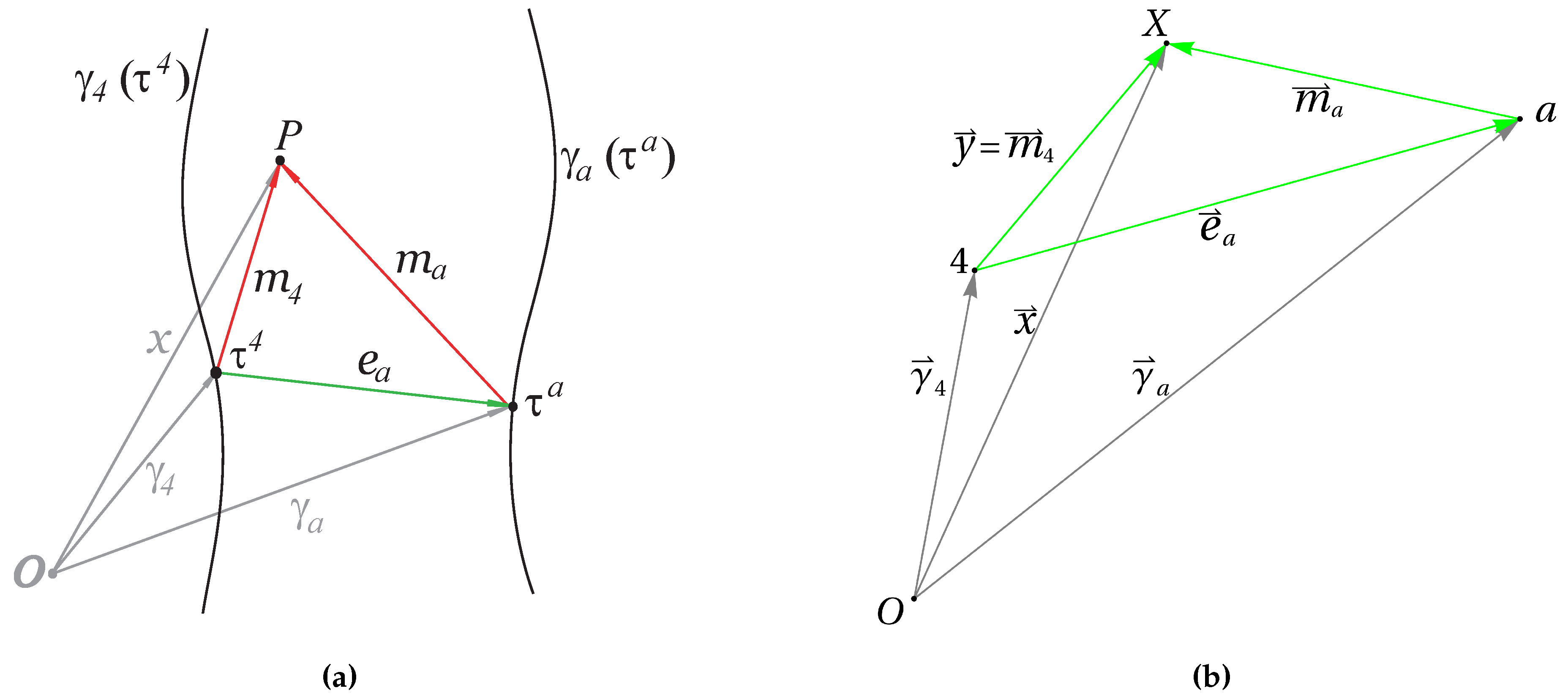
Table 1. Identifying Kleusberg’s notation and concepts with the time-like and space-like components of those of the RPS solution. In the last row,

μ = 1

(

μ = - 1

) stands for emission (reception) solutions.

Table 1. Identifying Kleusberg’s notation and concepts with the time-like and space-like components of those of the RPS solution. In the last row,

μ = 1

(

μ = - 1

) stands for emission (reception) solutions.

Kleusberg		RPS
pseudorange difference	$d_{a}$	$σ_{a}$	coordinate time difference
emitter distance to reference emitter	$b_{a}$	$\| {\vec{e}}_{a} \|$	emitter distance to reference emitter
unit vector from reference emitter to emitter a	${\hat{e}}_{a}$	$\frac{{\vec{e}}_{a}}{\| {\vec{e}}_{a} \|}$	unit vector from reference emitter to emitter a
user distance to emitter a	$s_{a}$	$\| {\vec{m}}_{a} \|$	user distance to emitter a
user distance to reference emitter	$s_{0}$	$\| \vec{y} \|$	user distance to reference emitter
unit vector from reference emitter to user	$\hat{e}$	$\frac{\vec{y}}{\| \vec{y} \|}$	unit vector from reference emitter to user
semi-difference	$\frac{1}{2} (b_{a}^{2} - d_{a}^{2})$	$Ω_{a}$	world-function scalar
three-vector	$\vec{G}$	$\frac{\vec{S}}{4 Ω_{1} Ω_{2} Ω_{3}}$	electric part of configuration bivector H
three-vector	$\vec{H}$	$\frac{\vec{B}}{μ 4 Ω_{1} Ω_{2} Ω_{3}}$	magnetic part of configuration bivector H

Disclaimer/Publisher’s Note: The statements, opinions and data contained in all publications are solely those of the individual author(s) and contributor(s) and not of MDPI and/or the editor(s). MDPI and/or the editor(s) disclaim responsibility for any injury to people or property resulting from any ideas, methods, instructions or products referred to in the content.

© 2024 by the authors. Licensee MDPI, Basel, Switzerland. This article is an open access article distributed under the terms and conditions of the Creative Commons Attribution (CC BY) license (http://creativecommons.org/licenses/by/4.0/).

Copyright: This open access article is published under a Creative Commons CC BY 4.0 license, which permit the free download, distribution, and reuse, provided that the author and preprint are cited in any reuse.

MDPI Initiatives

Important Links

Choose an area of interest and we will send you notifications of new preprints at your preferred frequency.

Disclaimer

Location Problem in Relativistic Positioning: Relative Formulation

Abstract

1. Introduction

2. Configuration of the Emitters Underlying Geometry

2.1. Splitting of γ A , m A and e a

2.2. Splitting of the Configuration Vector χ

2.3. Splitting of the Bivectors E a

2.4. Splitting of the Configuration Bivector H

3. The Location Problem

3.1. Splitting of the Particular Solution y ∗

3.2. Splitting of the Covariant Solution x

3.3. Emission Coordinate Domains and Bifurcation Problem

4. Kleusberg’s Solution

4.1. Concepts and Notation

4.2. Kleusberg’s Procedure to Obtain the Solution

4.3. Recovering Kleusberg’s from the Covariant Solution

5. Covariant Solution in Terms of the Principal Directions of H

5.1. Principal Directions of H Covariant Determination

5.2. Emission Coordinate Domains and Bifurcation Problem

5.3. User Location in the Region Where j Θ ( x ) = 0

5.4. Splitting of the Covariant Solution in Terms of l and n

6. Discussion and Comments

Author Contributions

Funding

Institutional Review Board Statement

Informed Consent Statement

Data Availability Statement

Acknowledgments

Conflicts of Interest

Appendix A. Notation

References

MDPI Initiatives

Important Links

Subscribe

2.1. Splitting of $γ_{A}$ , $m_{A}$ and $e_{a}$

2.2. Splitting of the Configuration Vector $χ$

2.3. Splitting of the Bivectors $E^{a}$

3.1. Splitting of the Particular Solution $y_{*}$

5.3. User Location in the Region Where $j_{Θ} (x) = 0$