Submitted:
04 June 2024
Posted:
05 June 2024
You are already at the latest version
Abstract
This paper introduces a three-layer system, proposing a comprehensive model of granular mixture transport over a mobile sloped bed in a steady flow. This system, consisting of the bottom, contact and upper zones, provides complete, continuous sediment velocity and concentration vertical profiles. The model considers gravity’s effect on sediment transport in the bottom (dense) layer, a crucial factor often overlooked in previous studies. The induced movement in the mobile sublayer of the dense layer causes an increase in velocity at the upper boundary of this layer, significantly affecting the vertical distributions of velocity and concentration above this layer. We described the interactions between fractions and an intensive sediment mixing and sorting process in the contact layer. The proposed shear variation, with an increase in its maximum value at the bed, adds to the novelty of our approach. The data sets used for the model’s validation cover various conditions, including slopes, grain diameters, densities and grain mobility conditions, from incipient motion to a fully mobilised bed. This extensive validation process instils confidence in the theoretical description and its applicability to real-world scenarios.
Keywords:
granular mixture
; steady flow
; sediment transport rate
; sediment velocity
; sediment concentration
; mobile sloped bed
1. Introduction
Structures such as dams significantly affect sediment transport conditions in rivers. Challenges arise in particular from the accumulation of sediment above the water level and erosion of the bottom downstream. To alleviate these problems, engineers develop various technical solutions, such as specialized sediment dams, bottom outlets or concrete channels to flush sediment downstream. Sedimentation in water bodies poses challenges not only from an engineering point of view (reduced retention capacity and the need for periodic dredging), but also for ecosystems (accumulation of pollutants, impeded biological self-cleaning, adverse effects on biota).
In addition to the problems of sedimentation in reservoirs, the construction of dam facilities involves the risk of downstream bed erosion. In order to counteract this, appropriate bottom stabilization measures are used and cascade dams can be built to raise water levels and reduce downstream flow velocities.
Key knowledge for engineers and designers includes sediment transport issues. Although engineers often resort to readily available empirical formulas for calculations of sediment transport, this approach can lead to errors due to still insufficient advanced theoretical models and appropriate numerical solutions.
1.1. Review of Literature
Recent research in sediment transport and hydraulic engineering focuses on various aspects of sediment management in rivers and reservoirs as well as modeling of these processes. In particular, the effects of hydraulic engineering structures on river morphology and methodologies for protecting against the negative effects of erosion and sedimentation are being studied.
One of the key topics is numerical modeling of hydraulic flushing in reservoirs for sediment management. Various methods such as drawdown flushing, pressure flushing, and turbidity current venting are discussed. The need for sediment management in reservoirs to maintain their retention capacity and functionality is emphasized [1].
Another area of research involves new approaches aimed at estimating total sediment transport capacity in rivers, taking into account the influence of hydraulic variables as well as flow and sediment conditions. The importance of understanding the critical flow velocities that determine the initiation of sediment transport, both in uplifted form and at the bottom in dragged form, is highlighted [2].
In addition, the literature review on modeling erosion and sediment transport indicates the significant implications of these processes for agricultural production, water quality, and changes in river channels. It is important to select an appropriate model for evaluation of these processes at the catchment scale, taking into account the spatial and temporal diversity of such phenomena [3].
These studies reveal the need for continued development of research methods and tools to better understand and manage morphodynamic processes in rivers and reservoirs, which is crucial for the design and maintenance of hydraulic infrastructure in the face of changing environmental conditions. Indeed, there is still no complete mathematical description of sediment transport that would allow reliable prediction over a wide range of hydrodynamic conditions, as pointed out by Berzi and Fraccarollo [4].
Classical formulas for calculating sediment transport, such as the Meyer-Peter and Müller formula [5], are inadequate under conditions of steep bottom slopes as they rely on the critical friction parameter [6], which varies with gradient.
In response to these challenges, authors such as Smart [7], Wong and Parker [8] and Cheng and Chen [9] have attempted to modify existing formulas by adjusting the value of critical Shields parameter for conditions of steep bottom slopes.
Graf and Suszka [10] developed their own empirical formula to adjust parameters for significant bottom slopes. Also, the studies of Recking et al. [11] and Parker et al. [12] focus on adjusting the value of critical Shields stress depending on bottom slope, grain diameter and other factors. However, Maurin et al. [13] emphasize that bottom slope may not affect only the value of the Shields [6] parameter, but many of the physical processes that accompany it.
Lamb et al. [14] presented a mathematical model based on vertical force equilibrium and a classical description of turbulence, emphasizing that at high bottom slopes, grain movement is more influenced by turbulence than bottom friction. In contrast, the study conducted by Park et al. [15] focuses on analyzing the effect of changes in the bottom level of mountain rivers on sediment transport using numerical and experimental models. These findings provide new data on the relationship between bottom structure and sediment transport in mountain rivers, taking into account a variety of flow and topography conditions.
A study by the Maritime Research Institute Netherlands [16] uses experiments in large wave channels to analyze the effect of bottom slope on beach morphological changes and sediment transport during different wave conditions. The results show how varying wave conditions can affect sediment transport processes in coastal zones.
Research by Chinese scientists [17] introduces a new methodology for measuring sediment transport capacity on steep slopes using a specially designed channel. This method allows for more accurate measurements of sediment transport capacity under different slope and flow conditions, which is crucial for modeling erosion on hillsides.
Tan W. and Yuan J. [18,19,20] described the experiments under sinusoidal oscillatory flows over a sloping bed. They argued that the effects induced by the bed slope on sediment transport may be as important as the effects due to the wave’s asymmetry.
Recently, Radosz et al. [21,22] have collected measurements on the vertical structure of sediment fluxes during the wave crest and trough phase over the sloped bed. The experimental work included measurements using the particle image method and measurements of sediment transport and granulometric distributions of sediments collected in the traps on both sides of the sloped initial area. The experimental data were compared with theoretical analysis based on a three-layer model of graded sediment transport in wave motion Kaczmarek et al. [23,24,25].
In summary, most authors focus either on modification or development of new formulas and mathematical models that will better describe the behavior of sediments at steep bottom slopes, with particular attention to the description of flow turbulence and the vertical structure of sediment transport.
1.2. Objective and Scope of Study
The aim of this study is to develop and experimentally verify a theoretical model for the transport and vertical structure of transport and segregation of non-cohesive and granulometrically heterogeneous sediments under steady flow conditions in an open channel. The model describes the transport of sediment over a bottom locally sloping in line with or opposite to the direction of sediment motion, ranging from zero to slopes close to the value of the angle of internal friction. The proposed theoretical model is validated with many data sets for different slopes, grain diameters and densities in a wide range of grain mobility conditions for incipient motion to a fully mobilized bed.
2. Materials and Methods
2.1. Theoretical Model Assumptions
Under flow conditions, sediment transport near the bottom occurs as a result of the energy imparted by the fluid in motion via shear stresses, which are a measure of friction against the bottom of fluid elements. Shear stress as the causal factor of sediment movement is described by friction velocity as follows:
where:
– is the water density.
The friction velocity is an input in modeling. In order to determine this friction velocity from the experiments it is proposed to find the friction velocity value from equation (2) for measured velocity profile:
where is the skin roughess assumed , is von Karmen constant (assumed as 0.40) and is median diameter. The vertical axis is directed upward with the origin at the bottom.
Under open channel flow conditions due to gravitational forces, shear stresses are a measure of friction against the bottom of a fluid element of depth (Figure 1):
where: is the slope of energy line, and is the earth’s acceleration.
Under steady-state uniform flow conditions (i.e., where the water depth, cross-sectional area and water velocity in each channel cross-section are constant), the energy line is parallel to the bottom slope (Figure 1), with the following relationships:
2.2. Three-Layer Transport Structure
Sediment transport varies in nature and is accompanied by different physical processes depending on the distance from the bottom to the free surface of the water. At the bottom, there are high concentrations and lower velocities, and there is an intensive exchange of momentum between sediment grains as a result of their collisions with each other. In the immediate vicinity of the bottom, there is sorting of grains, some of which fall back to the bottom, and the rest are transported in suspension, which occurs up to the free water level.
In relation to this variation in the nature of sediment transport along the depth, for steady flow conditions in an open channel, a three-layer description (Figure 1) was assumed following Kaczmarek et al. [24], which allows not only to determine the exact distribution of sediment concentration and velocity but also to map the sorting process of heterogeneous sediments. An arrangement of layers was proposed with a continuous description of concentration and velocity profiles in each layer.
The layer at the bottom, according to the assumptions below, has very high concentrations (dense layer) (Figure 1). Transport of highly “packed” grains occurs here, with the closer to the conventional bottom line, the greater the loosening of the water-soil mixture in a dense layer, and the exchange of momentum between grains occurs as a result of their collisions. In relation to the occurrence of high concentrations, it is assumed that all grain fractions move at a given ordinate with equal speed (have equal velocity profiles). This is because interactions between grains are very strong and individual fractions “pull” each other in a water-soil mixture of very high concentration.
The dense layer can be divided into two sublayers. The first, lower sublayer is very strongly “packed” with grains. There is plastic, “Coulomb” type stresses here. Transport of sediments begins in the higher sublayer of the dense layer, where the movement of the water-soil mixture takes place, and the exchange of momentum between grains occurs as a result of their collisions. Due to the very strong interactions between grains, it is proposed to describe the sediment transport in this sublayer with a single representative diameter .
Above the dense layer, there is further loosening of the water-soil mixture and exchange of momentum between grains in the process of collisions, with each th fraction of sediment in this area, characterized by the th concentration of , moves with its own separate th velocity . A process of grain sorting takes place here, with the finer grains remaining in suspension and being lifted higher by turbulence, while the coarser grains fall back to the bottom. This layer is called the contact layer.
The stresses between grains in the contact layer vary from a maximum value (at the interface between the dense layer and the contact layer) to the magnitude of at the upper boundary of contact layer (Figure 1). It is noteworthy that in the upper sublayer of dense layer, the stress component representing viscous stresses gradually disappears. The vanishing nature of viscosity-type stresses, characteristic in the presented model in the upper part of dense layer, was confirmed by Cowen et al. [26], who studied shear stress values under laboratory conditions.
The uppermost region is the suspension area (turbulent flow area), which is divided into inner layers (where the sediment velocity distribution is assumed to be logarithmic to which the calculated velocity profile inside the contact layer tends) and an outer layer with very low concentrations.
The boundary conditions between the layers, described by different equations, are defined in such a way that the distribution of sediment concentrations and velocities is continuous, practically from the zone of complete stillness to the area near the water surface, where the concentrations are already very small. At the upper boundary of the dense layer, the effective stresses are equal to:
where is the so-called mobile bottom effect parameter.
In order to determine the parameter , it was assumed that the total transport in dense and contact layers could be compared with the classical empirical formula of Meyer-Peter and Müller [5]. This formula was developed on the basis of a series of sand and gravel fraction transport measurements, has been extensively tested and is the most widely used in engineering practice for calculating the bedload transport, i.e. in this case for transport in the dense and contact layers.
Thus, a relationship can be formulated:
where: – sediment transport in dense layer being a function of friction ; – sediment transport in the contact layer being a function of friction ; – relative density, as a ratio of sediment density to water density, – dimensionless transport determined by the MPM formula:
where: – Shields’ critical parameter [6], assumed , and Shields’ dimensionless parameter defined as:
The parameter is determined iteratively from equation (6) [24,27,28,29].
2.3. Equations in the Dense Layer
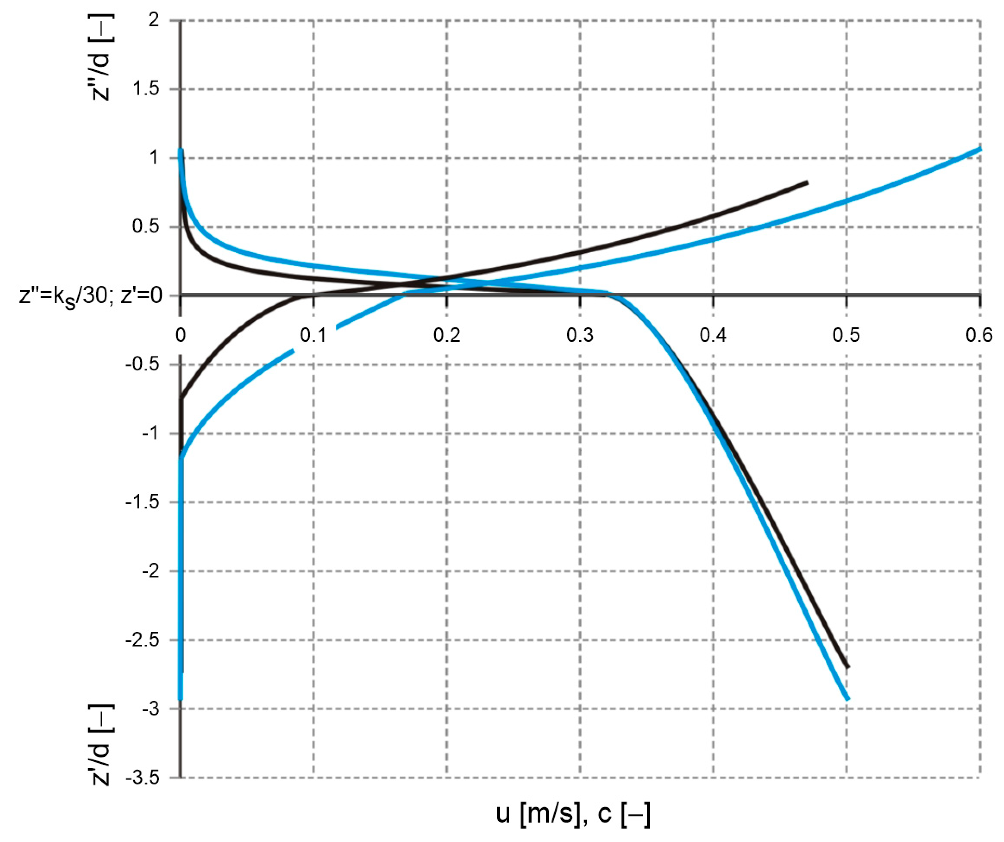
Consider the effect of gravitational forces on sediment grains resting on a bed of slope . The gravitational force on the grains can be divided into two components, i.e. parallel to the bottom , and perpendicular to the bottom (Figure 2).
As the bottom slope increases, the value of the component of gravity parallel to the bottom will increase, at the expense of decreasing component perpendicular to the bottom. Thus, the component parallel to the bottom will act together with shear stresses associated with water flow, causing an increase in sediment transport intensity (or the opposite, slowing transport, in the case of locally occurring reverse gradients). Taking the above into account, consider the components of gravitational forces (Figure 2) in the balance of vertical and horizontal forces of dense layer. The equations of dense layer in the coordinate system withaxis hooked to the line of theoretical bottom and points downward (Figure 2) then take the following form [30]:
where: , (constant); – maximum concentration value at the lower boundary of dense layer; – sediment concentration at the upper boundary of dense layer, = quasi-static angle of internal friction, = angle between the principal axis of stress and the horizontal axis:
, – concentration functions (following Sayed and Savage [31]) described as:
where: representative diameter in grain flow sublayer is assumed as .
The equations (9) and (10) are solved using the iterative method with numerical integration. The concentration , following [24], was adopted as the boundary condition at the upper boundary of dense layer. First, the course of concentration values is sought until the lower boundary condition is reached, i.e. the maximum concentration, which was adopted as [24]. The calculation is carried out only up to the point where . This is dictated by the need for the denominators in equations (12) and (13) not to reach zero. It is assumed that above this concentration value the grains are already maximally “packed” and remain motionless. Here, the boundary condition for velocity is assumed to determine the distribution of velocity throughout the dense layer for the previously calculated concentrations. Thickness of mobile part of the dense sublayer is determined for . Under intense flow conditions, the mobile sublayer is dominant and covers all or almost all of dense layer. Conversely, for weak hydrodynamic conditions, almost all of dense layer is affected by the relation , and the thickness of mobile sublayer practically corresponds to the diameters of individual transported grains.
Under conditions of significant bottom slope, there will be strong soil loosening in the bulk of dense layer. Thus, in this part, according to [24], it can be assumed . However, near the lower boundary of dense layer, it can be expected that the soil is much less loosened, and the angle of internal friction reaches values close to normative for the type of soil in the compacted state. Following Sobczak [30] it was assumed that the area of linear variation of the angle of internal friction from the magnitude of to the normative magnitude in the compacted state is contained in the interval between the thickness of loosened state estimated as the magnitude of (the thickness of mobile sublayer for a non-sloping bottom under very strong hydrodynamic conditions), and the thickness when the concentration in dense layer reaches the value for the compacted state.
Solving the equations inside the contact layer (and upward) for each th fraction leads to finding both the velocity , as well as the concentration . In this case, the axis is directed upward (Figure 2) due to the fact that the method of solution in these layers has been discussed in detail in papers [24] for homogeneous sediments and [29] for granulometrically heterogeneous sediments, and more recently in papers [27,28] for non-cohesive granulometrically heterogeneous sediments with cohesive additives, then the reader is referred to the mentioned papers for details of the solution.
At this point, it is only worth mentioning that the total sediment transport is calculated as follows:
where – is the share of particular th fraction in the grain size distribution, – is the number of fractions, and – is the thickness of the contact layer.
3. Discussion of Numerical Calculation Results
Figure 3a,b and Figure 4a,b show the calculated vertical distributions of sediment concentration and velocity in the contact and dense layers, respectively, at different bottom slopes ranging from -20 º to 20 º for identical flow and sediment parameters (, , ). It can be seen that changing the slope angle has a dramatic effect on both the concentration values inside the contact layer (Figure 3a) and upward, as well as on sediment velocities in this area (Figure 3b) and on velocities and concentrations inside the dense layer (Figure 4a,b). Negative gradients correspond to gradients opposite the flow direction. Of course, this is possible only in local, short sections of the bottom, where there are large bottom formations or underwater thresholds at which material accumulation has occurred. In such cases, the component of gravitational forces acting on the sediment grains parallel to the bottom will act opposite to the shear stresses associated with the flow. The results presented here show that in such a case both the concentrations, velocities and thicknesses of the active (mobile) sublayer inside the dense layer are significantly smaller compared to situations with a positive gradient.
Figure 3a.
Calculated vertical distributions of sediment concentration in the contact layer at different bottom slopes for equal flow and sediment parameters (, , ).
Figure 3a.
Calculated vertical distributions of sediment concentration in the contact layer at different bottom slopes for equal flow and sediment parameters (, , ).
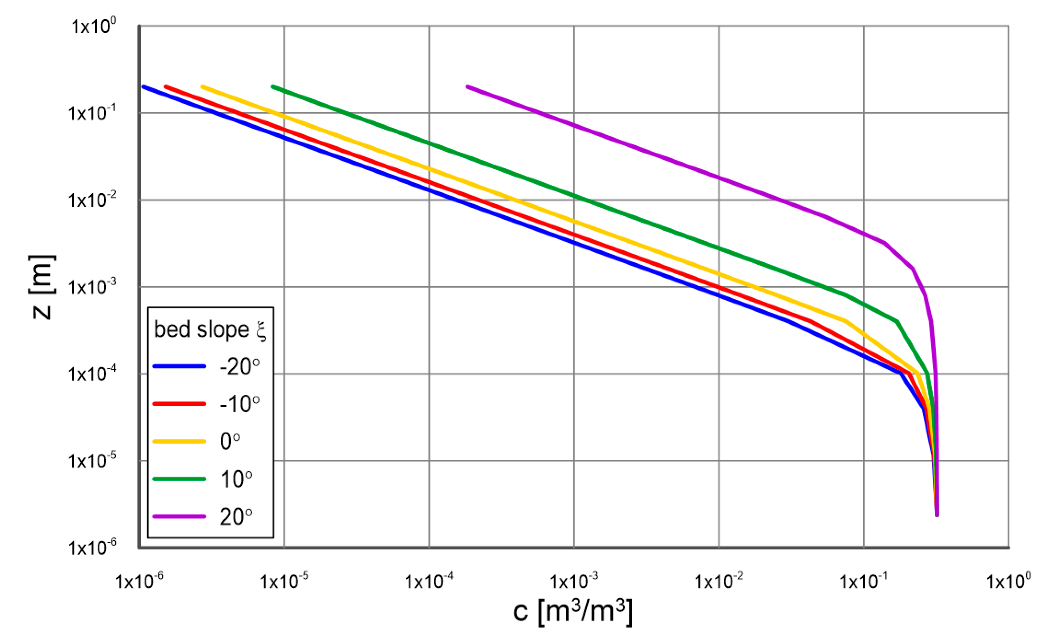
Figure 3b.
Calculated vertical distributions of sediment velocity in the contact layer at different bottom slopes for equal flow and sediment parameters (, , .
Figure 3b.
Calculated vertical distributions of sediment velocity in the contact layer at different bottom slopes for equal flow and sediment parameters (, , .
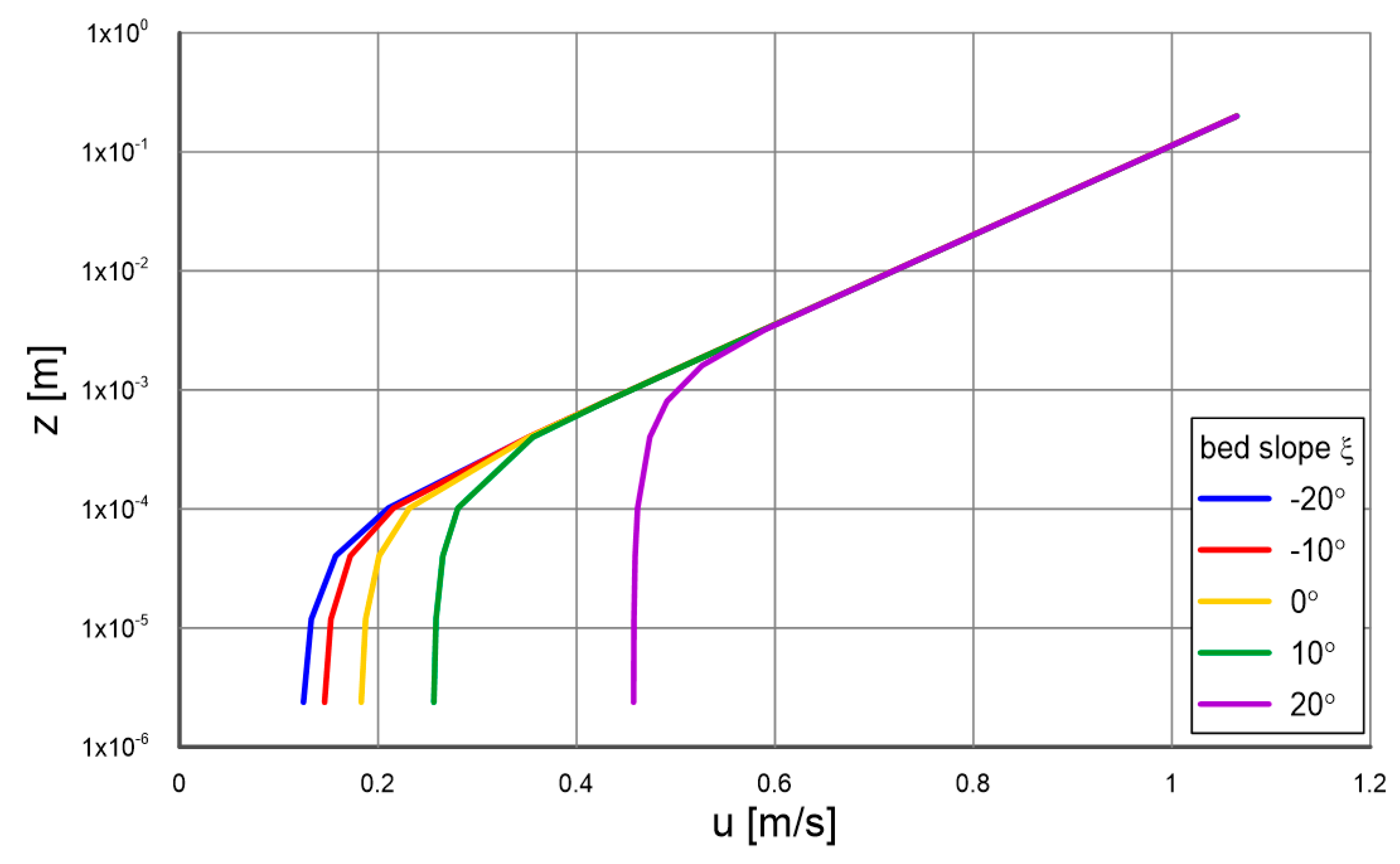
Figure 4a.
Calculated vertical distributions of sediment concentration in the dense layer at different bottom slopes for equal flow and sediment parameters (, , .
Figure 4a.
Calculated vertical distributions of sediment concentration in the dense layer at different bottom slopes for equal flow and sediment parameters (, , .
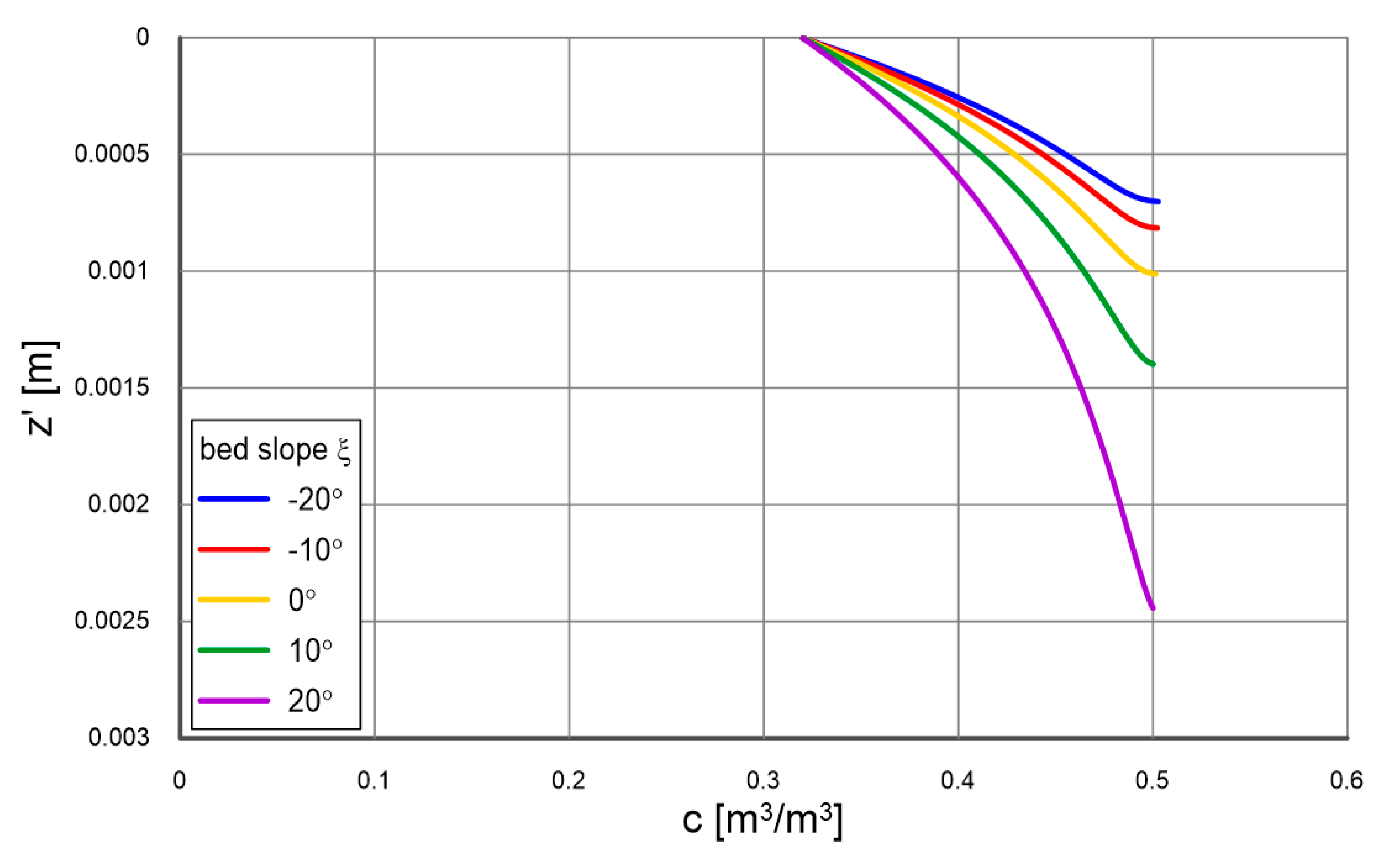
Figure 4b.
Calculated vertical distributions of sediment velocity in the dense layer at different bottom slopes for equal flow and sediment parameters (, , .
Figure 4b.
Calculated vertical distributions of sediment velocity in the dense layer at different bottom slopes for equal flow and sediment parameters (, , .
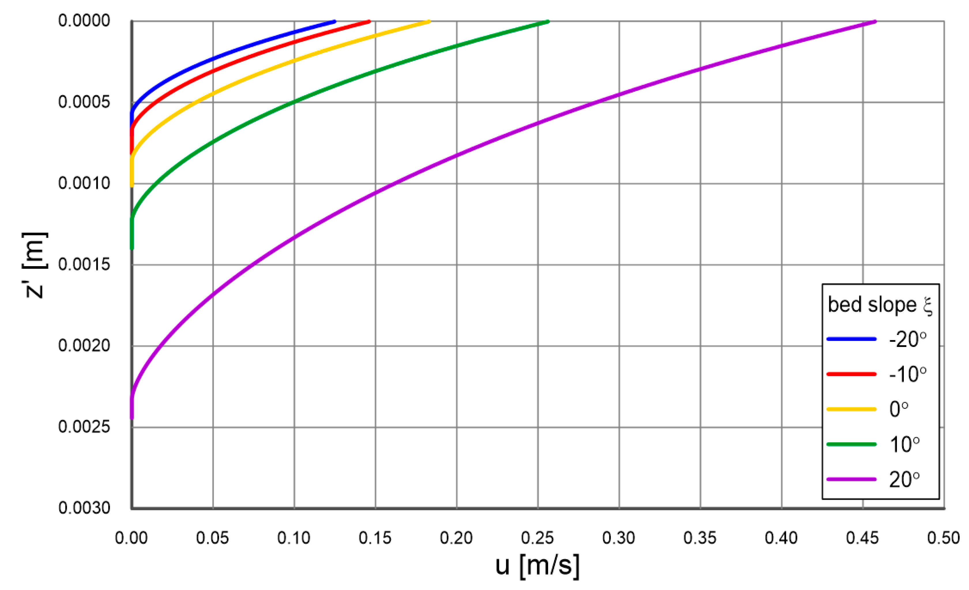
Figure 5 shows the calculated transport intensities in dense layer and the contact layer and upward at different bottom slopes for the present case (, , ). It is interesting that as the bottom slope increases, the increase in transport values in the contact layer is more intense than in the dense layer. This is because the model satisfactorily reproduces the greater “loosening” of sediments in the bottom in the case of significant slopes. Therefore, the presented example results of transport calculations are intuitive and reasonable, as the result of such “loosening” greater transport will occur in the contact layer, due to the dramatic increase in velocity at its lower boundary, where transport is dominated by momentum exchange via grain collisions. As a result, there will also be significantly higher concentrations of suspended sediment further from the bottom (Figure 5).
Figure 5.
Calculated sediment transport in the dense and contact layers for different bottom slopes with equal flow and sediment parameters (, , ).
Figure 5.
Calculated sediment transport in the dense and contact layers for different bottom slopes with equal flow and sediment parameters (, , ).

4. Discussion of Calculation Results in Comparison with Measurements
4.1. Vertical Profiles of Velocity, Concentration and Grain Size Distribution
This section may be divided by subheadings. It should provide a concise and precise description of the experimental results, their interpretation, as well as the experimental conclusions that can be drawn.
Frey [32] conducted measurements under laboratory conditions for homogeneous surrogate sediment consisting of glass beads with a diameter of at a constant gradient of , under flow intensities corresponding to dimensionless friction in the range . He carried out the observations using a special camera that allows recording images at 130 frames per second. However, in order to record individual grains selectively, the width between the vertical panes of flow channel walls was chosen to ensure that there was only one “vertical” layer of beads.
In order to compare the measurement results with calculations for specific conditions, calculations were carried out with the three-layer model presented in this paper.
Figure 6a (following [30]) shows the original vertical distributions of both velocity and concentration presented by Frey [32] for four measurement series, designated by the author as N10-x, where 10 stands for the bottom slope in percentage and is the designation of the specific measurement series under given conditions. Calculation results of these quantities with the multilayer model for selected series are shown in Figure 6b. The calculated concentration and velocity distributions for two measurement series are shown: N10-6 for and N10-16 for, with fixed diameter and bottom slope of 10%. The data presented are calculation results in 3 layers of the model, i.e. in the dense layer ( axis pointing downward) and in the contact layer and upward ( axis pointing upward).
Figure 6a.
Vertical distributions of velocity and concentration determined by Frey [32] for four measurement series: N10-6 (black points), N10-8 (red points), N10-16 (blue points) and N10-20 (green points).
Figure 6a.
Vertical distributions of velocity and concentration determined by Frey [32] for four measurement series: N10-6 (black points), N10-8 (red points), N10-16 (blue points) and N10-20 (green points).
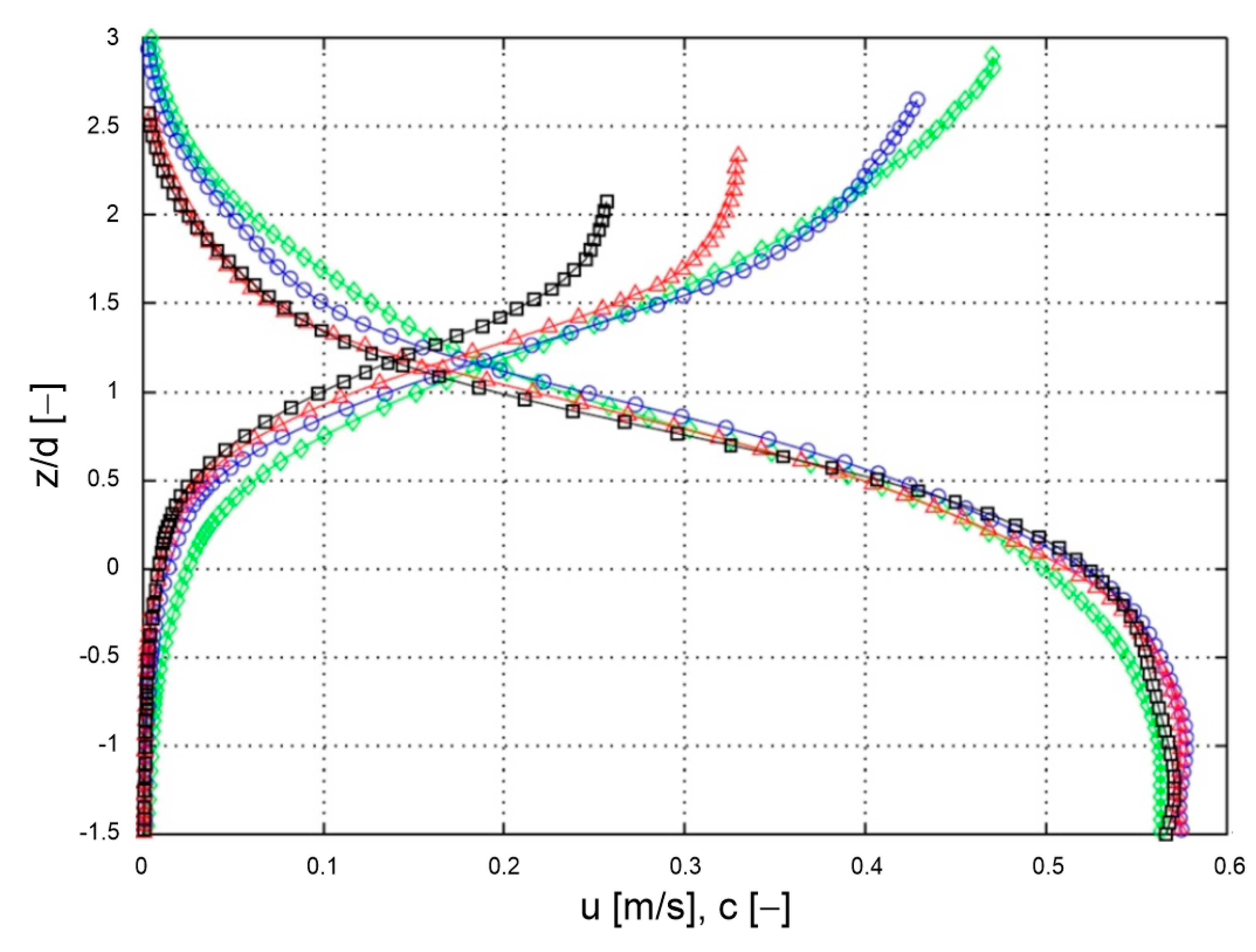
Figure 6b.
Calculated velocities and sediment concentrations with the multilayer model for parameters corresponding to tests N10-6 (black lines) and N10-16 (blue lines).
Figure 6b.
Calculated velocities and sediment concentrations with the multilayer model for parameters corresponding to tests N10-6 (black lines) and N10-16 (blue lines).
It should be noted that the maximum concentration boundary values adopted for the calculations differ slightly from the measured values at the lower boundary of dense layer . However, this does not fundamentally affect the transport due to the zero sediment velocities occurring in this area. Comparing the calculation results (Figure 6b) with the corresponding distributions determined by Frey [32], shown in Figure 6a, it can be seen that the nature of velocity and concentration distributions are very similar. This confirms the validity of theoretical assumptions made for the lowest layers of the model, from the motionless zone, through the layer to the suspension zone.
There are, of course, some differences, with the model’s overestimation of sediment velocity in the upper zone shown in the figure being particularly noticeable. However, it is difficult to clearly address the model’s errors, as the tests took place on surrogate sediment of balls of equal diameter transported in a single vertical layer. Under such conditions, the real dynamics of grains (here – glass balls) is greatly influenced by the channel walls in the immediate vicinity.
Sediment velocities and concentrations in the dense layer are mapped much better than in the contact layer. This may be related to the fact that this area is dominated by strong interactions between grains. Therefore, the above-mentioned effect of wall influence is most likely no longer as important as it is during fusion and faster grain movement. In the contact layer and upward, the calculated grain velocities are overestimated, because under natural conditions grains collide with other grains, with similar velocities – while in the laboratory measurements described by Frey [32], grains transported in one vertical layer “bump” against the channel walls, which are at rest. Therefore, friction is of great importance here under laboratory conditions and has the effect of slowing down the beads.
The calculated concentration values in the contact layer seem to decrease much more intensively with the distance from the boundary of two layers. However, it should be noted that the transport intensities calculated with the presented model in comparison with the transports calculated on the basis of Frey’s measurements [32] (Figure 7) provide satisfactory results.
In summary, when taking into account the measurement conditions, as well as the fact of replacing real sediment with glass beads, it can be stated that the consistency of measurement results with calculations is satisfactory.
One of the more interesting papers describing the vertical distribution of sediment concentration and segregation is the study by Damgaard et al. [33], who conducted measurements of fine sand transport by determining concentration and velocity profiles in a channel that allows the implementation of a bottom slope. They made measurements using granulometrically heterogeneous sediments with a median under conditions of dimensionless friction, varying the bottom slope from .
Figure 7.
Example transports of sediments represented by 6 mm diameter glass beads measured by Frey [32] under 10% bottom slope conditions against the results of calculations (following [30] with the presented multilayer model. The points from lowest to highest represent successive tests for dimensionless friction values, respectively: , , and.
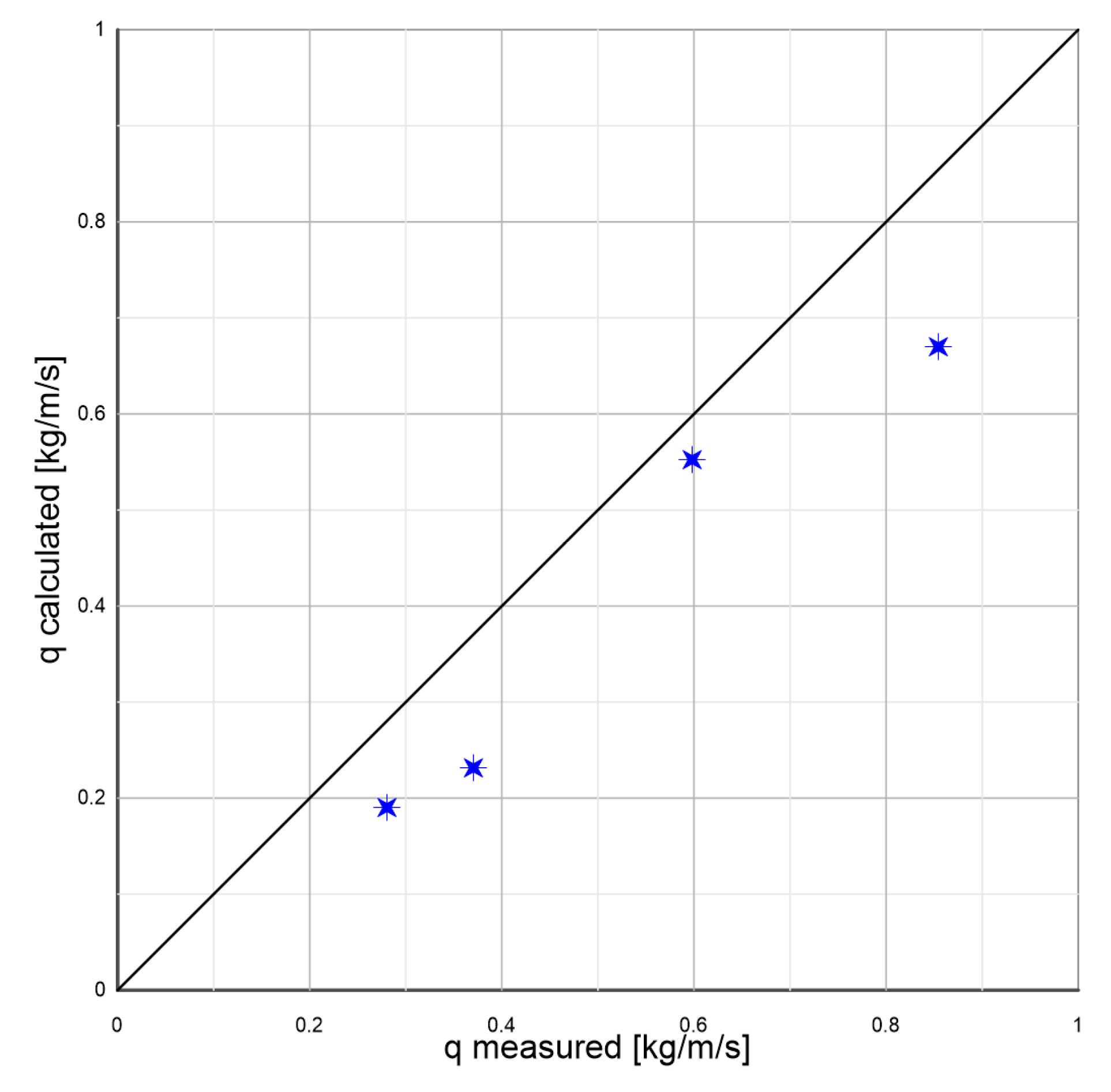
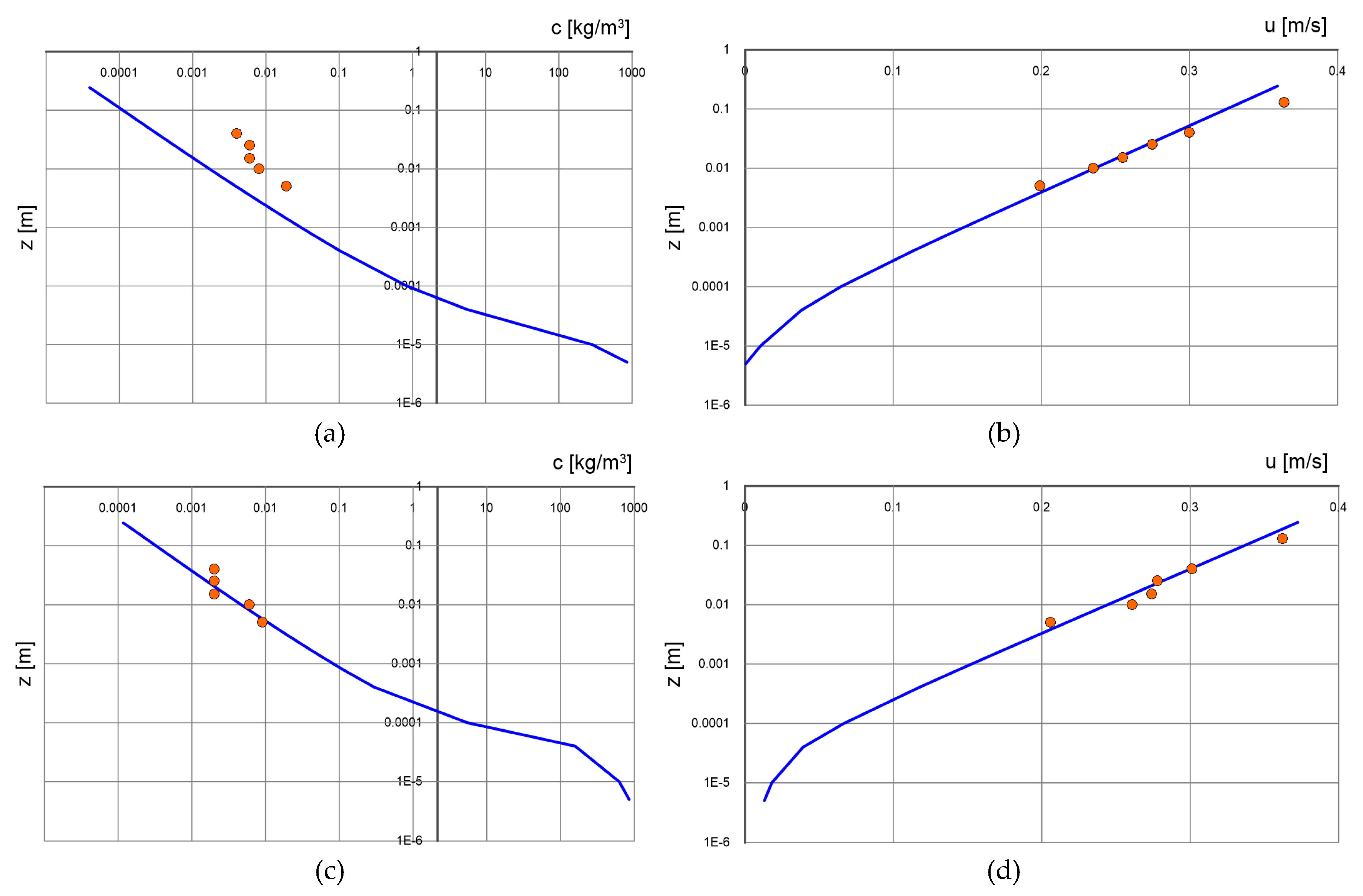
Figure 8 and Figure 9 show a comparison of calculation results with measurements of velocity and concentration distributions for conditions defined by the dimensionless friction . The first figure shows results for gradients consistent with the direction of flow, and the second figure shows results for opposite gradients (marked with “-”). It can be seen that the model reflects sediment velocities very well and reproduces concentration distributions well. The highest concentration correspondences are found for significant gradients (), while for smaller gradients () relatively large differences are observed, which are most likely due to the presence of bottom forms (ripples), which are particularly strong at smaller gradients.
Figure 8.
Comparison of calculated with three-layer model (lines, contact layer and outer layer) and measured (points) by Damgaard et al. [33] distributions of velocity and sediment concentration for different bottom slopes . (, ): (a), (b) ; (c), (d) ; (e), (f).
Figure 8.
Comparison of calculated with three-layer model (lines, contact layer and outer layer) and measured (points) by Damgaard et al. [33] distributions of velocity and sediment concentration for different bottom slopes . (, ): (a), (b) ; (c), (d) ; (e), (f).
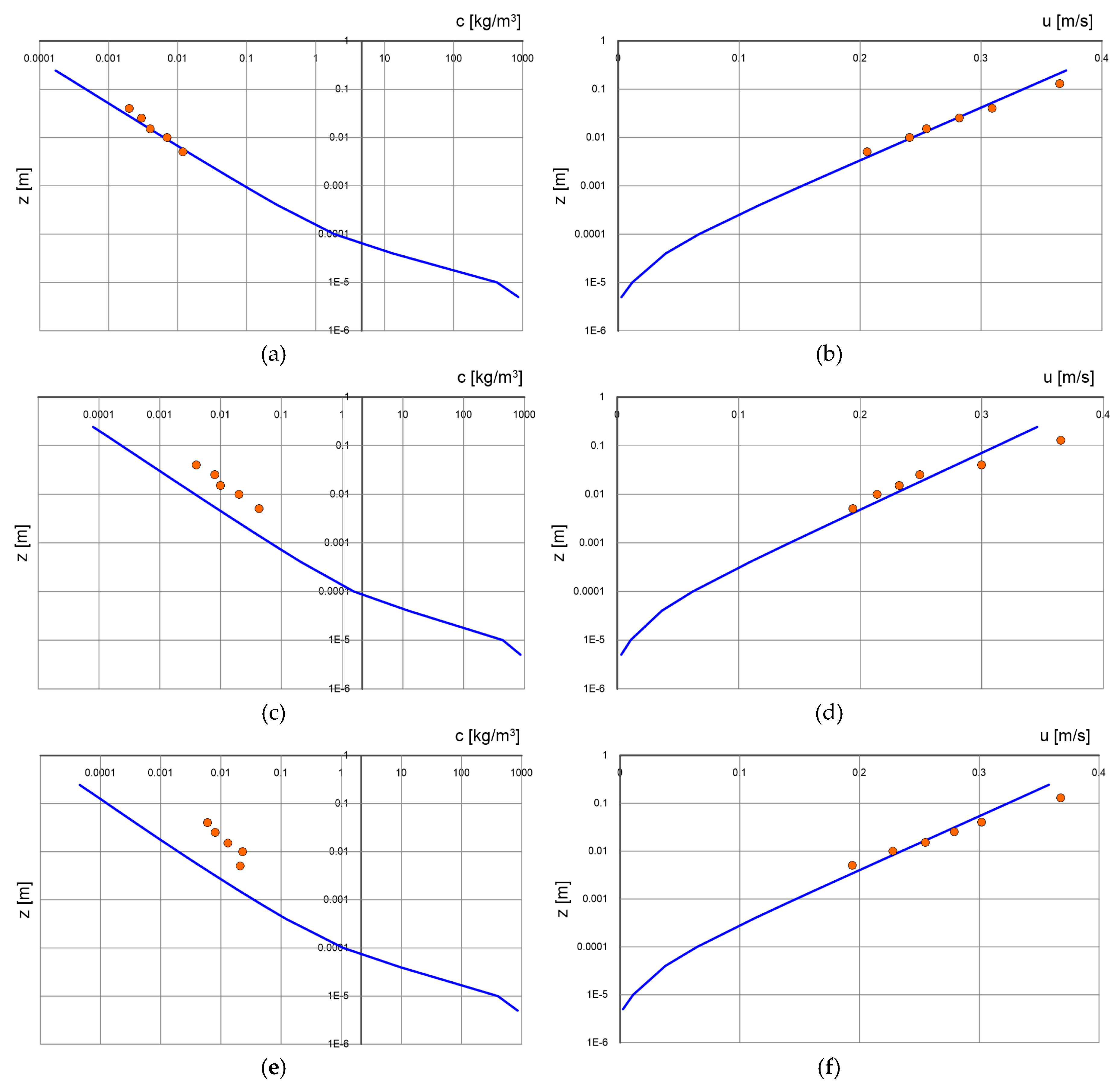
Figure 9.
Comparison of calculated with multilayer model (lines, contact layer and outer layer) and measured (points) by Damgaard et al. [33] distributions of velocity and sediment concentration for bottom slopes opposite the flow direction (, ): (a), (b) ; (c), (d) .
Figure 9.
Comparison of calculated with multilayer model (lines, contact layer and outer layer) and measured (points) by Damgaard et al. [33] distributions of velocity and sediment concentration for bottom slopes opposite the flow direction (, ): (a), (b) ; (c), (d) .
Damgaard et al. [33] also devoted attention to the vertical segregation structure of heterogeneous sediments under conditions of different bottom slopes. The authors measured the concentration of individual sediment fractions at different distances from the bottom and presented the results in the form of vertical variation of the characteristic diameter . The parameters corresponding to each test (values of dynamic velocity, dimensionless friction and bottom slope) are shown in Table 1. Calculation results against the measurement results for selected series are shown in Figure 10 and Figure 11, with the vertical variation of the median of suspended sediments at height was calculated from the obtained concentration distributions according to the equations:
Knowing the calculated fractional content at a given level it is easy on this basis to estimate the median .
The lines represent the calculation results, and the points represent the values of d50 from measurements, i.e. obtained from the measured concentrations of individual fractions. The lowest value of the lines representing calculation results (), corresponds to the characteristic diameter of the sediment at the bottom. As can be seen in figures, the quality of prediction of the vertical structure d50 in the area above the intensive sorting zone is a test of the validity of theoretical assumptions and the adopted sorting model in the layers below.
Figure 10.
Calculated vertical distributions of the variation of characteristic diameter (lines) against the measurement results by Damaard et al. [33] (points) for conditions of bottom slope (tests 1, 2, (a), (b)) and (tests 4, 5, 6, (c), (d), (e)) for different conditions of dimensionless friction /see Tab. 3[M1] /. The measured diameter of sediment at the bottom .
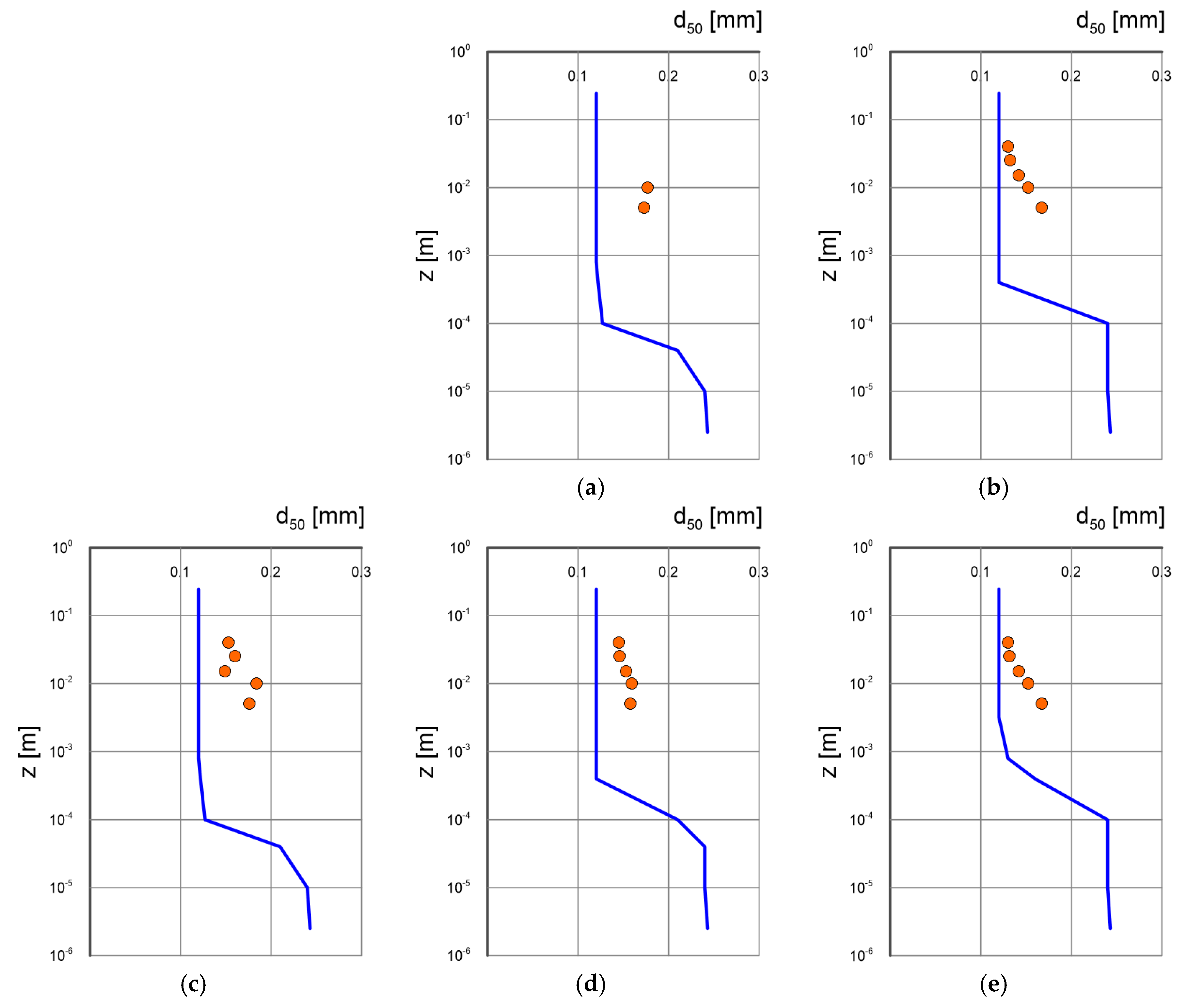
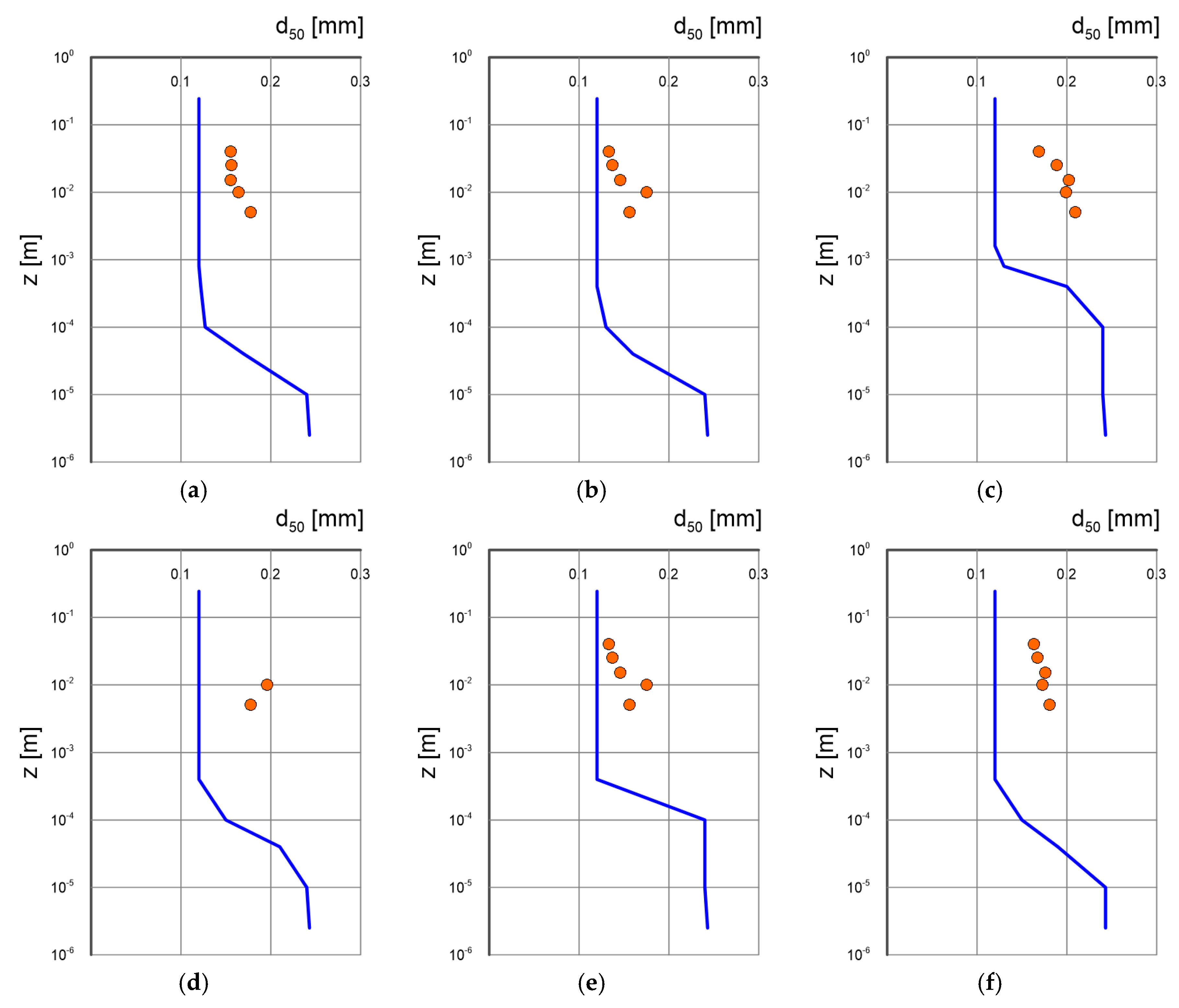
Figure 11.
Calculated vertical distributions of the variation of characteristic diameter (lines) against the measurement results of Damaard et al. [33] (points) for conditions of bottom slope (tests 10, 11, 12, (a), (b), (c)) and (tests 13, 14, 15, (d), (e), (f)) for different conditions of dimensionless friction /see Tab. 3/. The measured diameter of sediment at the bottom .
4.2. Sediment Transport
Luque [34] conducted a series of measurements of sediment transport in a channel 8m long, 20cm high and 10cm wide with a design that allowed for a bottom slope. Flow in the channel was generated using a pump. Measurements were conducted for flow with no slope (0º) and three different bottom slopes: 12º, 18º and 22º under conditions of dimensionless friction in the range . The author studied transport of heterogeneous sediments, which he described by characteristic diameters . Measurements for the verification of presented model are very interesting, as Luque [34] used a wide range of materials representing sediments both in terms of not only diameters, but also density:
- sand with density and diameters and ;
- gravel with density and diameter ;
- particles of shelled walnut with density and diameter ;
- magnetite grains with density and diameter .
To calculate shear stresses, the authors measured water velocity distributions. Sediment transport was determined using an optical method, based on analysis of recorded films made for grains traveling a certain distance in a given time.
For the direct values of shear stress and sediment and bottom slope characteristics presented by Luque [34], calculations were conducted with the model presented in this paper. Comparisons of calculated and measured transport intensities expressed in terms of dimensionless transport are shown in Figure 13, Figure 14, Figure 15, Figure 16 and Figure 17. The solid lines indicate a correspondence of the calculation results with the measured data, while the dashed lines indicate the limits of double determination error. The dimensionless transport according to equation (6) is defined as follows:
Figure 12.
Comparison of calculated and measured transport intensities for sandy sediment with a diameter and density under conditions of different bottom slopes; (based on Luque’s laboratory studies [34]).
Figure 12.
Comparison of calculated and measured transport intensities for sandy sediment with a diameter and density under conditions of different bottom slopes; (based on Luque’s laboratory studies [34]).
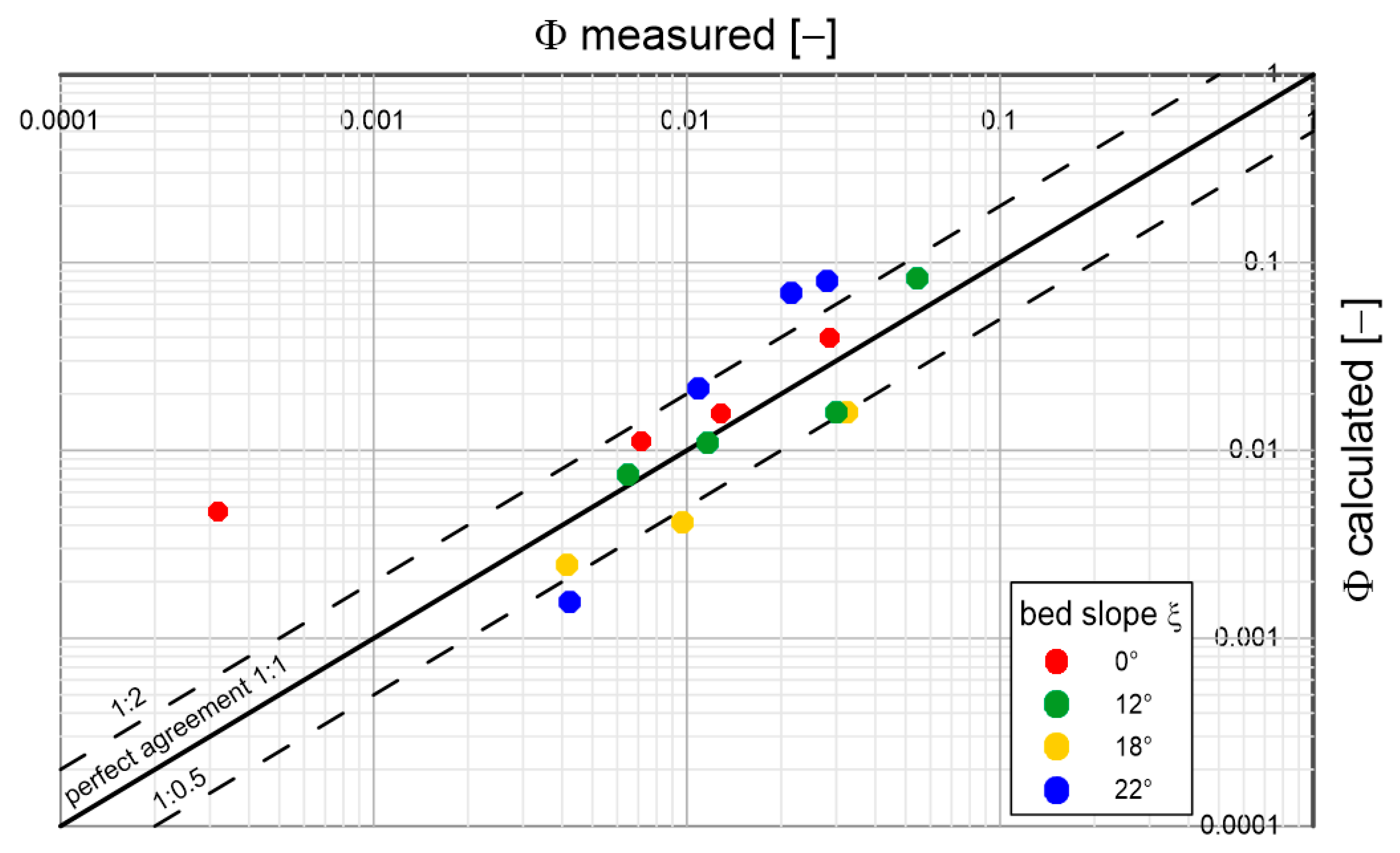
Figure 13.
Comparison of calculated and measured transport intensities for sandy sediment with a diameter and density under conditions of different bottom slopes; (based on Luque’s laboratory studies [34]).
Figure 13.
Comparison of calculated and measured transport intensities for sandy sediment with a diameter and density under conditions of different bottom slopes; (based on Luque’s laboratory studies [34]).
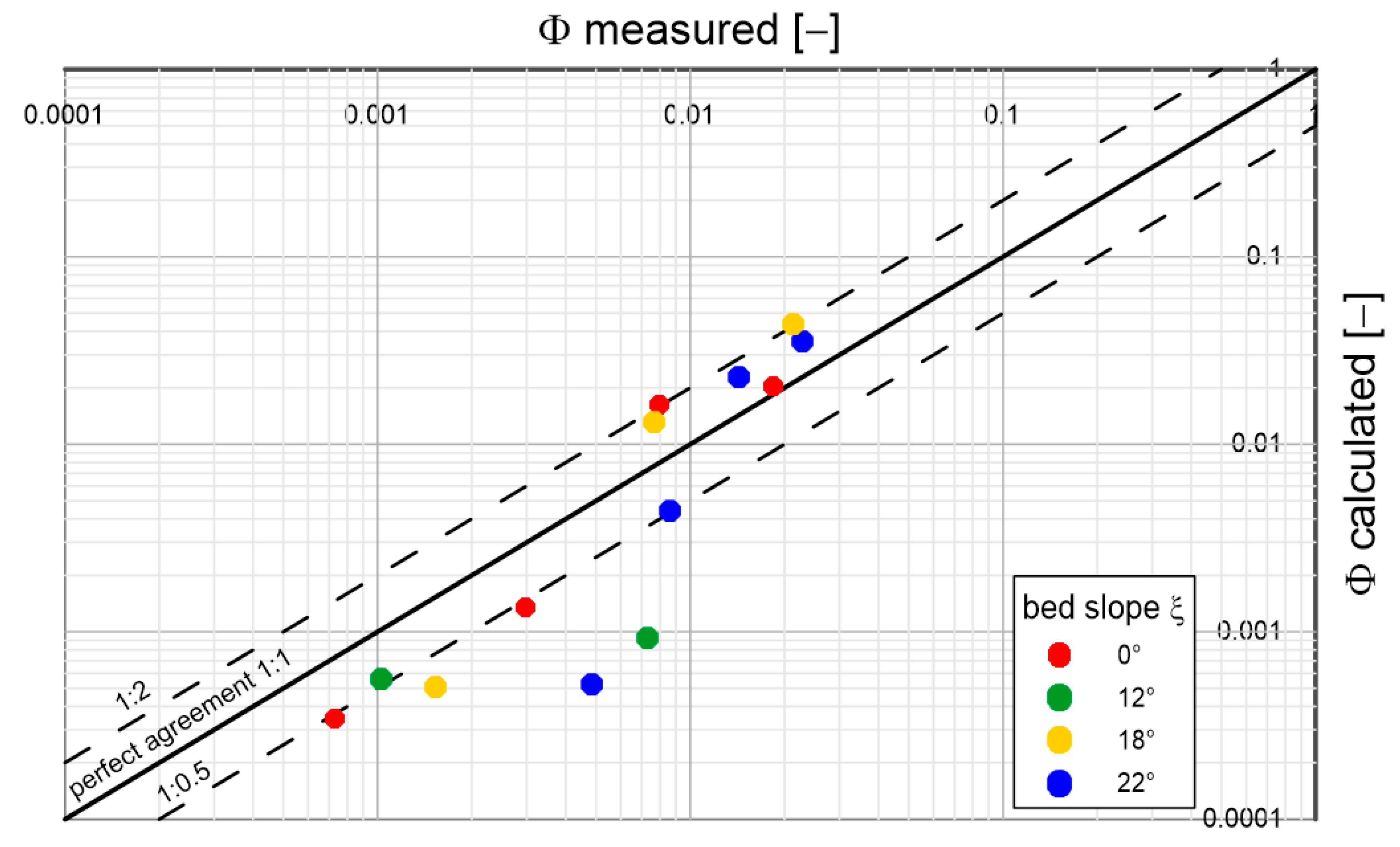
Figure 14.
Comparison of calculated and measured transport intensities for sandy sediment with a diameter and density under conditions of different bottom slopes; (based on Luque’s laboratory studies [34]).
Figure 14.
Comparison of calculated and measured transport intensities for sandy sediment with a diameter and density under conditions of different bottom slopes; (based on Luque’s laboratory studies [34]).
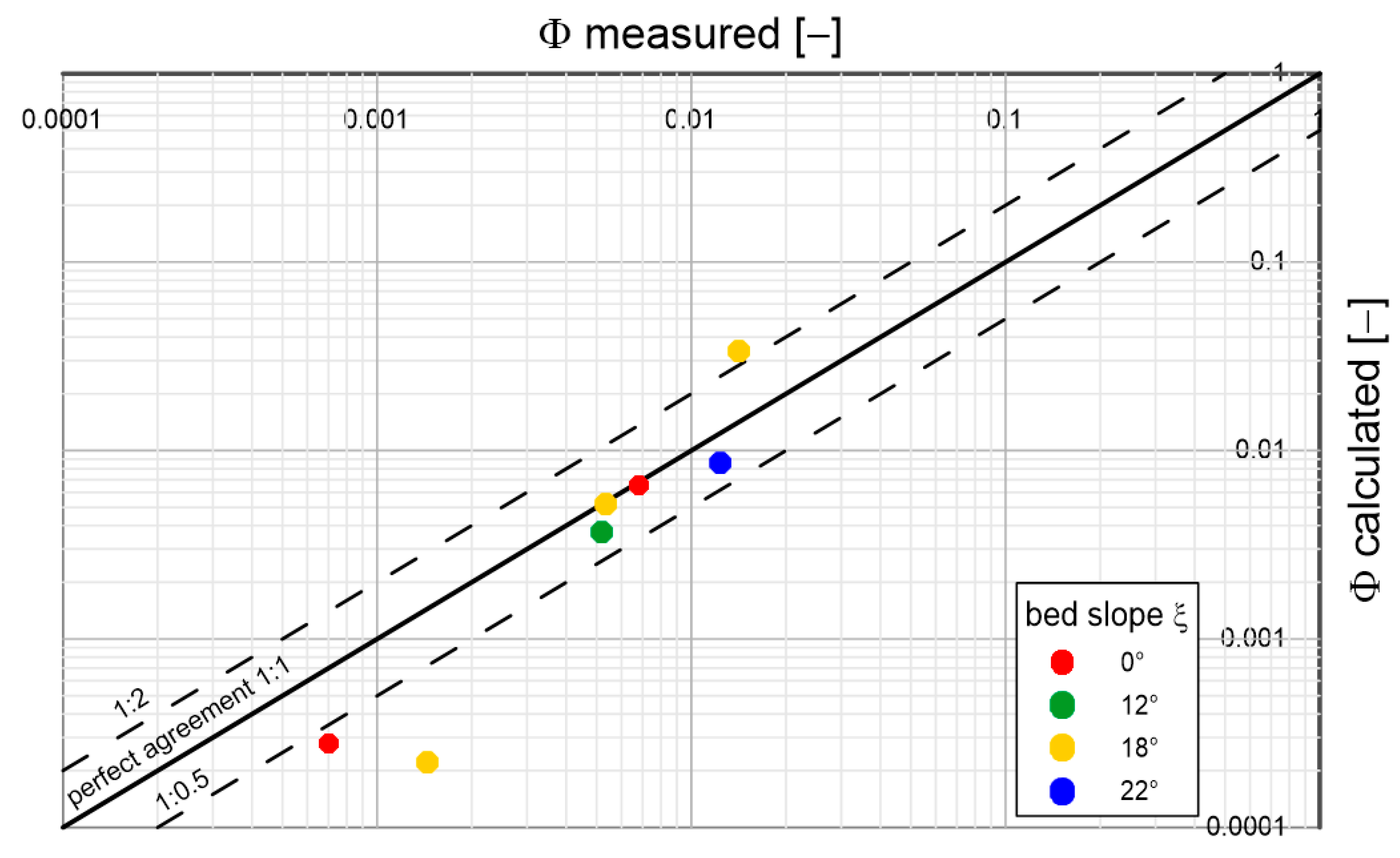
Figure 15.
Comparison of calculated and measured transport intensities for sandy sediment with a diameter and density under conditions of different bottom slopes; (based on Luque’s laboratory studies [34]).
Figure 15.
Comparison of calculated and measured transport intensities for sandy sediment with a diameter and density under conditions of different bottom slopes; (based on Luque’s laboratory studies [34]).
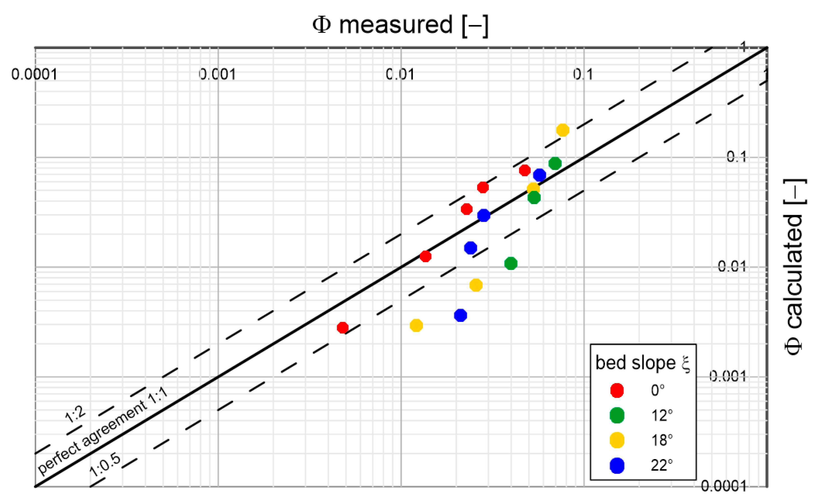
Figure 16.
Comparison of calculated and measured transport intensities for sandy sediment with a diameter and density under conditions of different bottom slopes; (based on Luque’s laboratory studies [34]).
Figure 16.
Comparison of calculated and measured transport intensities for sandy sediment with a diameter and density under conditions of different bottom slopes; (based on Luque’s laboratory studies [34]).
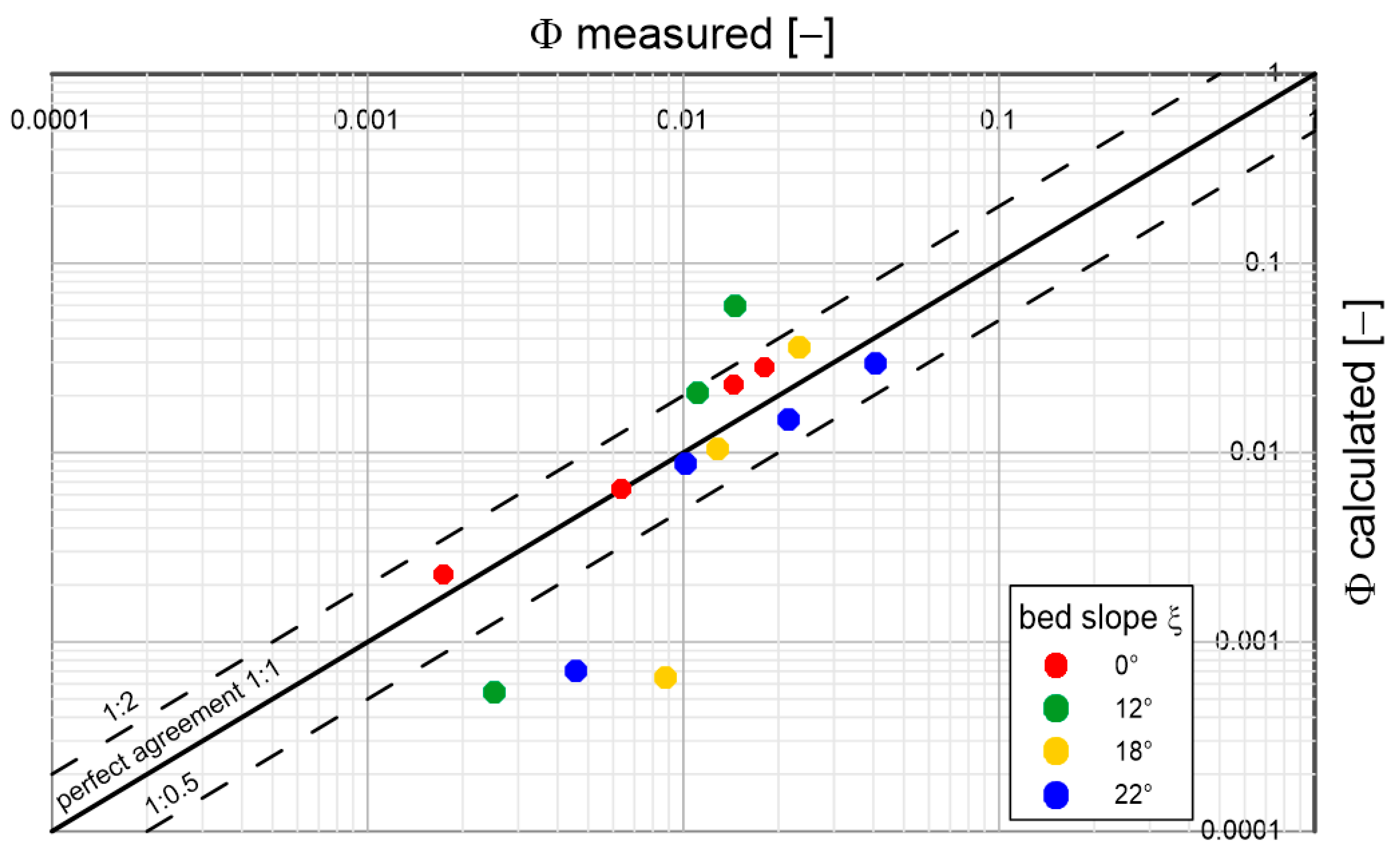
Figure 17.
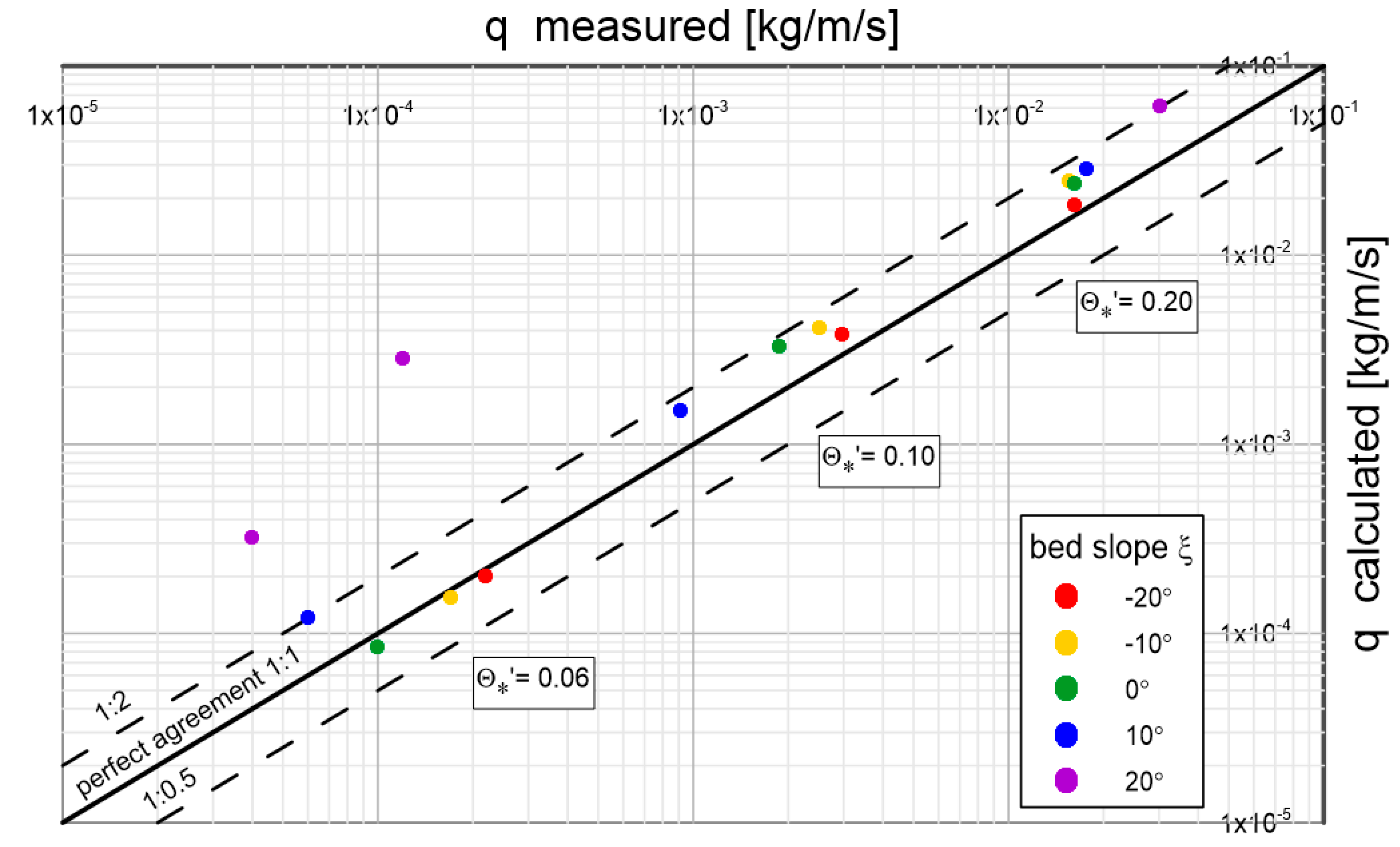
Results of sediment transport calculations compared with measured data by Damgaard et al. [33] for sediment with diameter of under conditions of dimensionless friction with gradients ranging from -20º to 20º.
Figure 17.
Results of sediment transport calculations compared with measured data by Damgaard et al. [33] for sediment with diameter of under conditions of dimensionless friction with gradients ranging from -20º to 20º.
Analysing the results shown in the above graphs, it can be concluded that the model reproduces sediment transports quite well, regardless of diameter and density, over the full range of bottom slopes used in the experimental studies. Most of the prediction results do not exceed double determination errors. It is worth mentioning that the results of Lugue measurements [34] are characterised by significant deviations from the average values of measurement series. Under conditions close to the beginning of sediment movement, such deviations are typical. Therefore, it is not possible to speak unequivocally about the error of calculation results here. It is interesting to note that there is no decisive difference in the quality of prediction of typical (sandy) sediments from substitute sediments with atypical densities (several times lower or higher). This is a good indication of the model, which may consequently have important implications for future engineering applications.
Figure 17 shows a comparison of calculated sediment transport values with selected measured data from Damgaard et al. [33] for heterogeneous sediment with diameter under conditions of dimensionless friction with gradients ranging from to . From Figure 17, it can be seen that the data in the graph are arranged in three groups, corresponding to 3 different flow conditions according to the dimensionless friction values described in the graph . A very good consistency between calculation results and measurements was obtained.
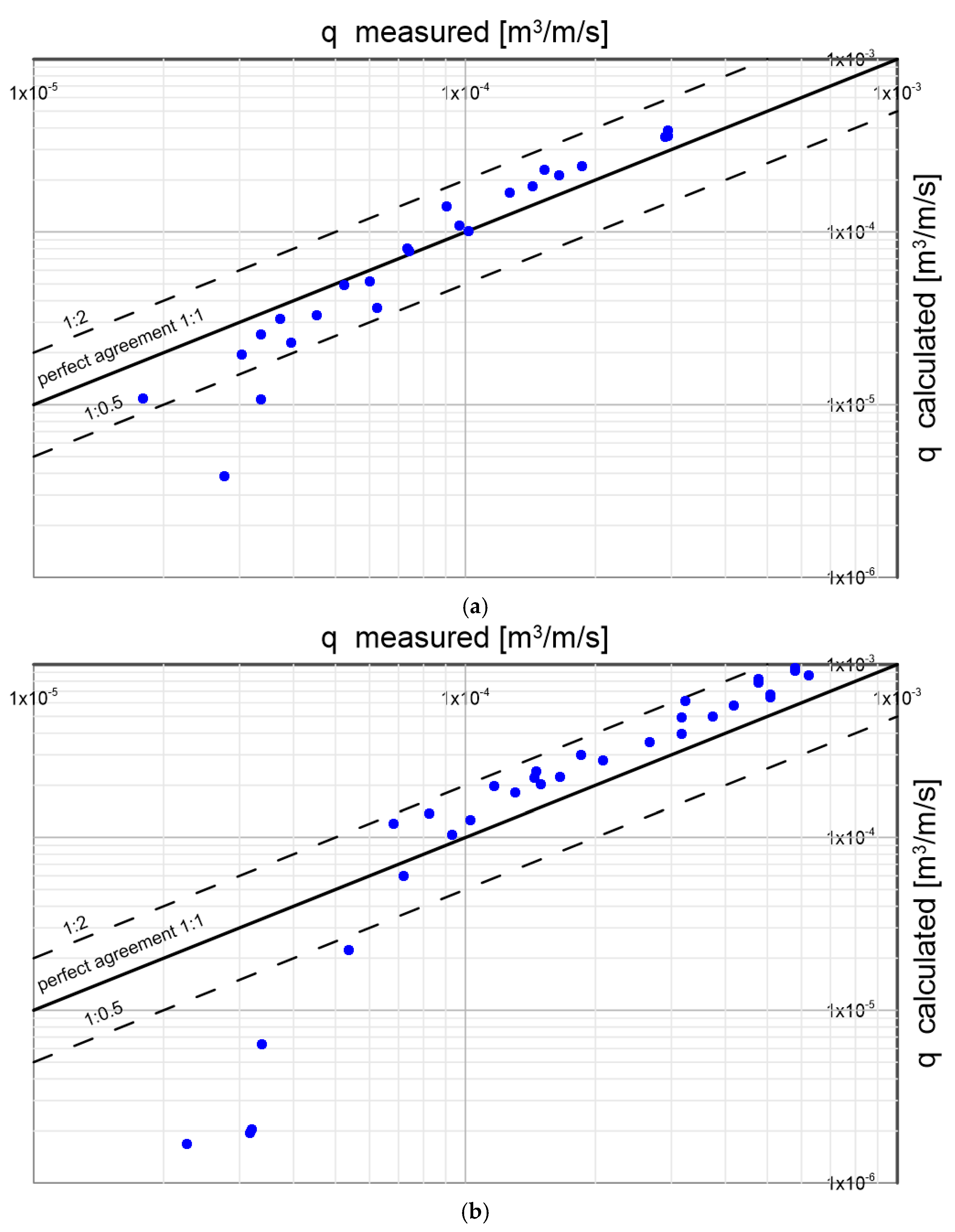
Further results of laboratory measurements that were used to verify the presented model under conditions of higher gradients were published by Smart and Jaeggi [35]. The authors conducted measurements of dragged sediment transport using a design that allowed the bottom to slope up to 40º.
Smart and Jaeggi [35] conducted transport measurements of four types of gravels with the following parameters: and density , and density , and density , and density , with bottom slopes of 3, 5, 7, 10, 15 and 20% for different values of dimensionless friction in the range .
A comparison of calculation results with measurements is shown in Figure 18. Satisfactory conformity was obtained, and in the case of the finest sediments () very good conformity. It should be noted that the most deviating results (, the lowest extreme point on the graph) were achieved for conditions at the boundary of the beginning of the movement, where concentrations are very small, and the measurements are usually characterized by significant scatterings of the results (single grains starting movement).
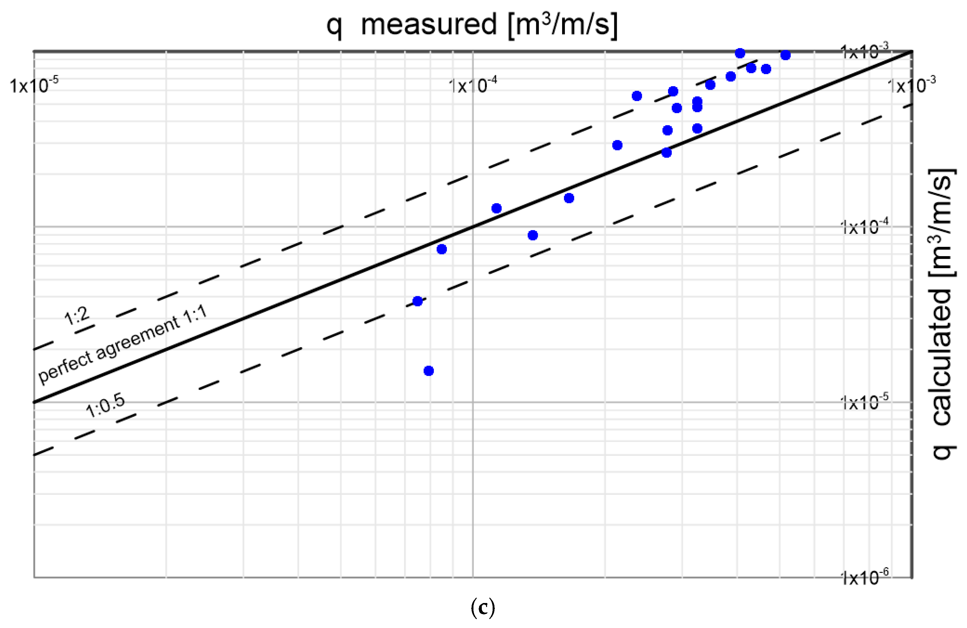
Larionov et al. [36] published the measurement results of sediment transport, which they conducted in a channel that allowed the realisation of slopes up to In the experiments they used 4 different heterogeneous sediments with characteristic diameters . Tests were carried out for the full range of dimensionless friction in the range from values close to the onset of grain motion (), with small bottom slopes close to , to strongly developed, intensive transport (max. value with bottom slopes up to ). Figure 19 shows a comparison of the measured results with the values calculated with the three-layer model. The consistency is satisfactory. In most cases, the results are within double determination error.
Aziz and Scott’s [37] measurement results were also used to verify the presented three-layer model under bottom slope conditions. Figure 20 shows a comparison of calculated sediment transport intensities for selected measurement results carried out by the authors for sediment with a diameter of , with bottom slopes of 3% and 10%, corresponding to two groups of dimensionless friction values in the range and . Again, very good conformity of calculation results with measured values was obtained.
Recking et al. [11] conducted measurements of homogeneous sediment transport granulometric in a circulation channel for bottom slopes of 0-10% in the range of conditions from the beginning of movement () to developed transport (). Calculation results against measured data for selected 3 diameters () are shown in Figure 21. The model reproduces the measured transport values very well. The exceptions are the lowest points, concerning measurements under conditions close to the beginning of debris movement ( close to the value of 0.06), when practically single grains are mobile. However, under such conditions, there are also significant discrepancies in the measurements.
Figure 18.
Comparison of sediment transport values calculated by three-layer model with the results of Smart and Jaeggi’s measurements [35] for four different diameters and different values of dimensionless friction in the range in the range of bottom slopes from 3 to 20%.
Figure 18.
Comparison of sediment transport values calculated by three-layer model with the results of Smart and Jaeggi’s measurements [35] for four different diameters and different values of dimensionless friction in the range in the range of bottom slopes from 3 to 20%.
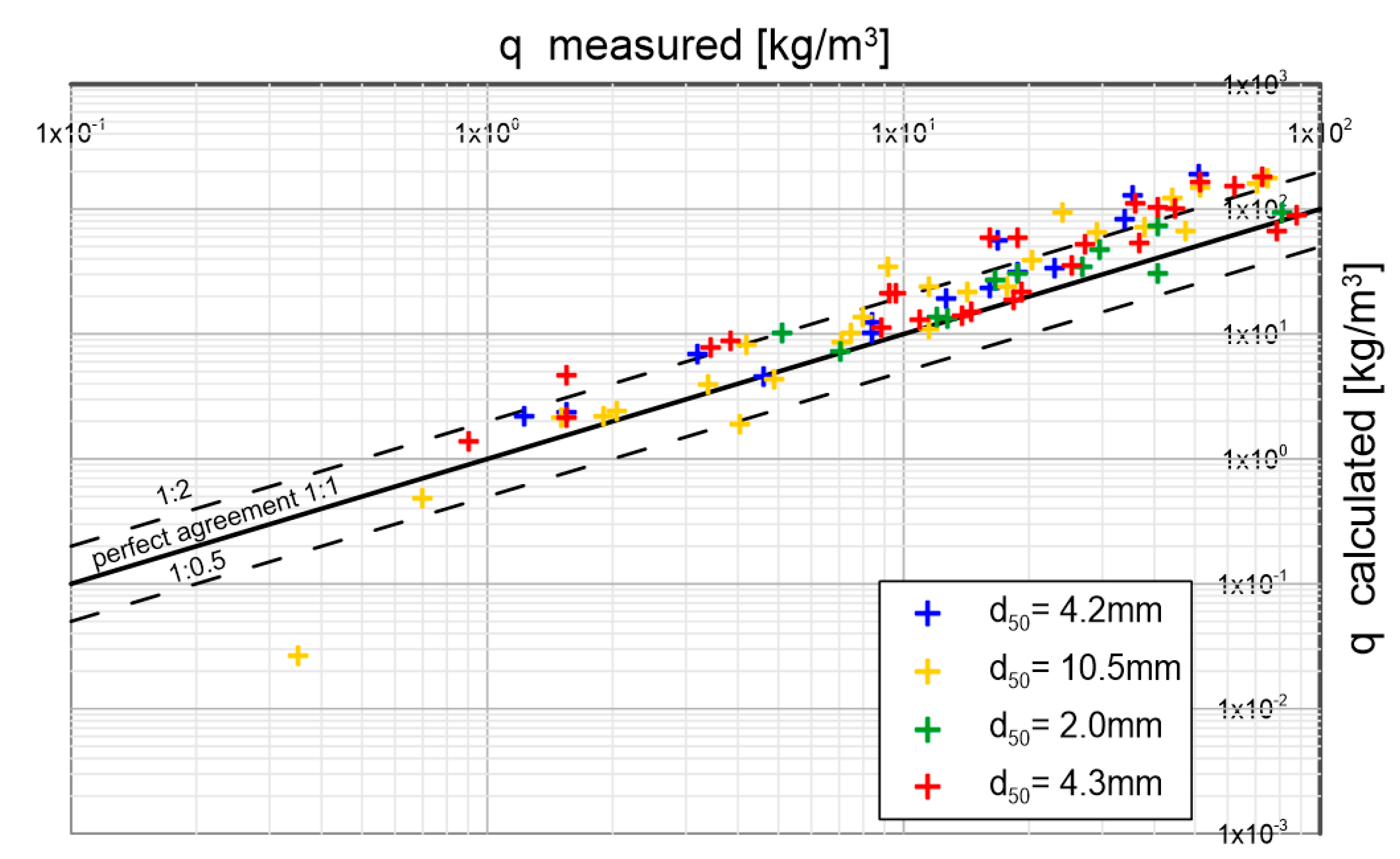
Figure 19.
Measurement results of Larionov et al. [36] in relation to sediment transport values calculated with the presented three-layer model for four selected diameters in the range of variation of dimensionless friction under conditions of bottom slopes from 0.5% to 35%.
Figure 19.
Measurement results of Larionov et al. [36] in relation to sediment transport values calculated with the presented three-layer model for four selected diameters in the range of variation of dimensionless friction under conditions of bottom slopes from 0.5% to 35%.
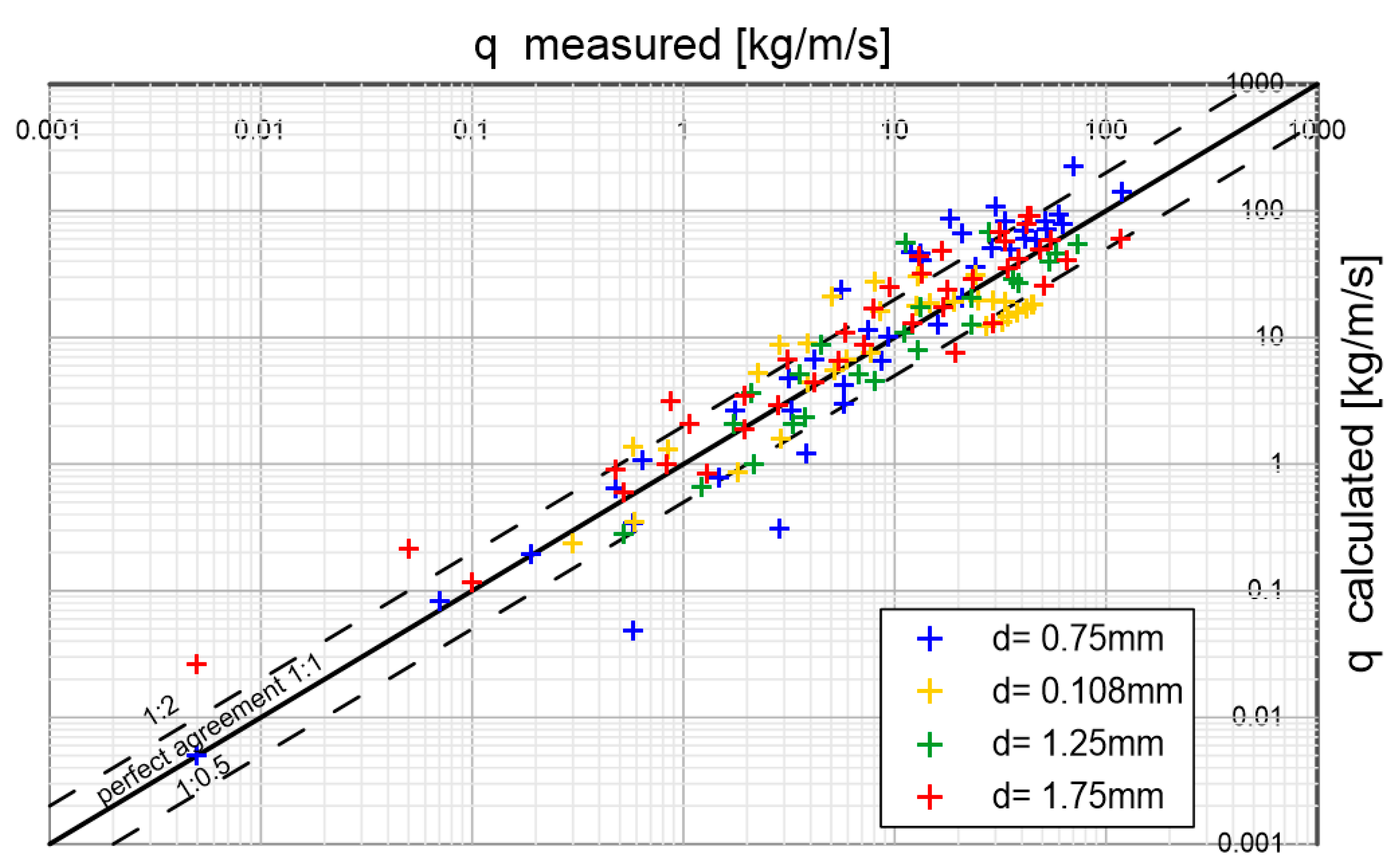
Figure 20.
Comparison of example results of Aziz and Scott [37] measurements of diameter sediment transport intensity for two different bottom slopes: 3% (black dots) and 10% (circles) in the dimensionless friction range with the results of three-layer model calculations.
Figure 20.
Comparison of example results of Aziz and Scott [37] measurements of diameter sediment transport intensity for two different bottom slopes: 3% (black dots) and 10% (circles) in the dimensionless friction range with the results of three-layer model calculations.
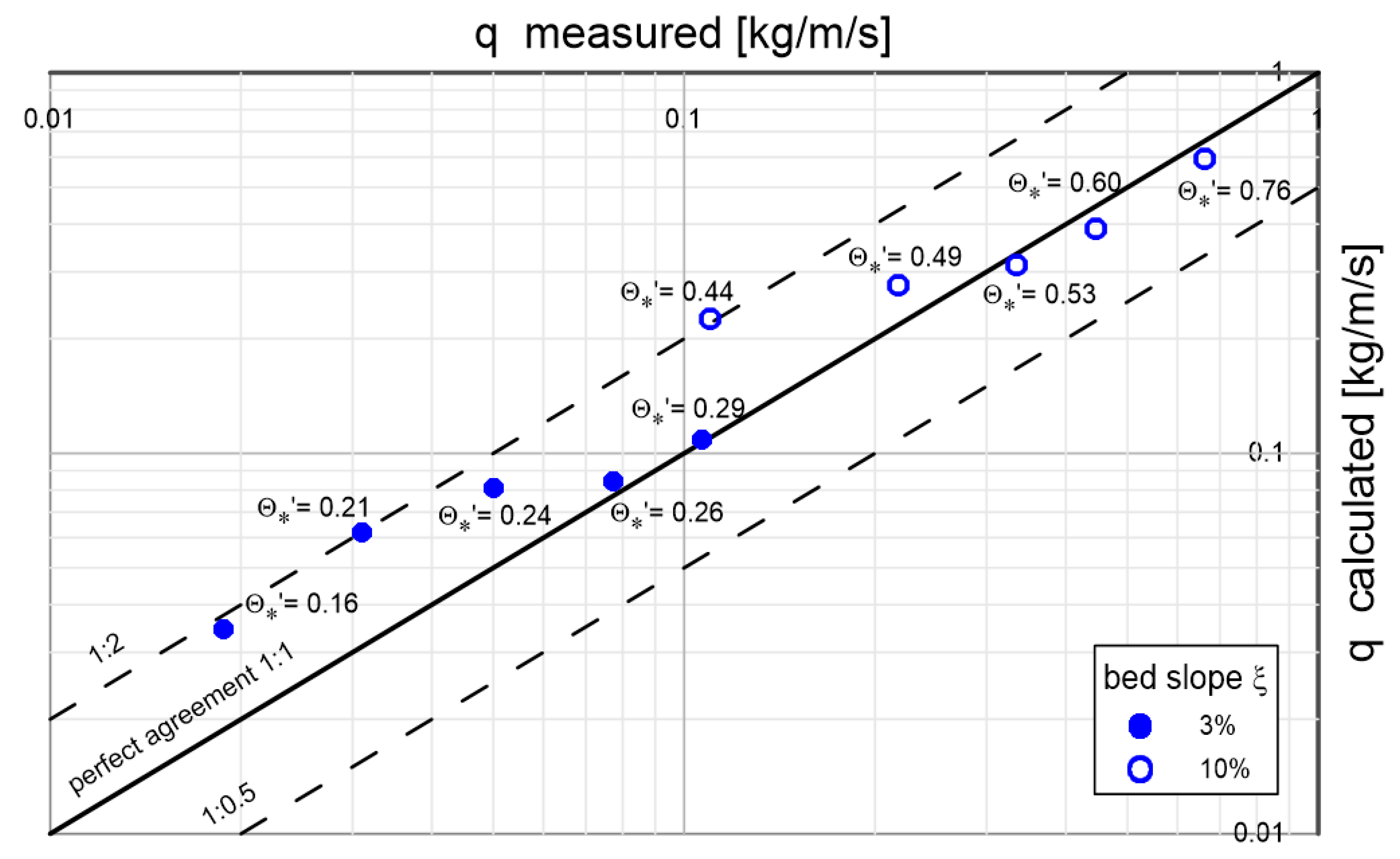
Figure 21.
Comparison of measured by Recking et al. [11] values of sediment transport for three diameters under conditions of slopes from 0% to 10% in the range of dimensionless friction with the results of calculations with the multilayer model: (a) ; (b) ; (c) .
Figure 21.
Comparison of measured by Recking et al. [11] values of sediment transport for three diameters under conditions of slopes from 0% to 10% in the range of dimensionless friction with the results of calculations with the multilayer model: (a) ; (b) ; (c) .
5. Conclusions
The paper presents an innovative three-layer model for the description of granular sediment transport over a mobile bed with a variable slope in a steady flow. The influence of gravity on sediment movement in the lower layer is discussed in detail, which is crucial for understanding the mechanisms of sediment grain movement in rivers and hydraulic channels. This influence is very often overlooked in previous studies. The presented model allows describing the vertical structure of transport and segregation of non-cohesive and granulometrically heterogeneous sediments under steady flow conditions in an open channel over a bed locally inclined in line with or opposite to the direction of sediment movement, in the range from zero to slopes close to the value of internal friction angle. Therefore, the proposed model enables to better understand and predict sediment behavior, which is crucial in the context of hydrotechnical infrastructure design and water resources management.
The model based on three-layer structure of sediment transport allows for a very detailed description of sediment behavior under different flow conditions. The paper identifies three main layers: bottom, contact and upper layers, each with different characteristics of sediment transport and concentration. This segmentation allows for a better analysis and understanding of the interactions between the layers, which is fundamental for accurate modeling of natural processes.
The authors particularly emphasize the role of gravity in sediment transport in the lower layer (dense layer). Gravity has the effect of loosening the bottom and increasing the thickness of lower layer and thus increasing the velocity at the upper boundary of this layer, which significantly affects the distribution of velocity and sediment concentration in the layers above. Understanding this mechanism is important for understanding the role of gravitational forces in sediment transport.
In this study, sediment transport over a bed with different slopes, from flat to slopes close to the angle of internal friction of the sediment, was modeled. The results of sediment transport modeling were compared with the results of experimental studies, obtaining a concordance of the results within double determination error.
In conclusion, the model presented in the paper offers an advanced tool for analyzing and predicting sediment behavior under varying hydraulic and morphological conditions.
Successful validation of the model for a very wide range of empirical data, including different slope types, grain diameters, densities and grain mobility conditions, provides a strong basis for applying the model to real engineering conditions. The model has the potential to support decisions on water resources management, optimization of water infrastructure operation, and minimization of risks associated with erosion and material deposition in river and reservoir systems. Thus, the model’s application in engineering practice can lead to significant improvements in the design of hydraulic infrastructure such as dams, barrages, bridges, and irrigation and flood control systems.
Author Contributions
Conceptualization, L.M.K., J.B., M.P., and I.R.; methodology, L.M.K. and J.B.; formal analysis, L.M.K., J.B., M.P. and I.R.; investigation, L.M.K., J.B., M.P. and I.R.; resources, L.M.K., J.B., M.P. and I.R.; writing—original draft preparation, L.M.K., J.B., M.P. and I.R.; writing—review and editing, L.M.K., J.B., M.P. and I.R.; supervision, L.M.K.; project administration, J.B., M.P. and I.R.; funding acquisition, L.M.K., J.B., M.P. and I.R. All authors have read and agreed to the published version of the manuscript.
Funding
The research was financially supported by the research project of the Koszalin University of Technology Faculty of Civil Engineering, Environmental and Geodetic Sciences: Dynamika niespoistego, niejednorodnego granulometrycznie ośrodka gruntowego w przepływie stacjonarnym i ruchu falowym w warunkach silnie nachylonego dna—funds no.: 524.01.07; project manager: L.K.
Institutional Review Board Statement
Not applicable.
Informed Consent Statement
Not applicable.
Data Availability Statement
The data presented in this study are available upon request from the corresponding author.
Conflicts of Interest
The authors declare no conflict of interest.
References
- Lai, Yong G. et al. Hydraulic Flushing of Sediment in Reservoirs: Best Practices of Numerical Modeling. Fluids 2024 vol. 9, no. 2, p. 38. [CrossRef]
- Shmakova, M. Sediment Transport in River Flows: New Approaches and Formulas [Internet]. Modeling of Sediment Transport. IntechOpen; 2022. Available from: http://dx.doi.org/10.5772/intechopen.103942. [CrossRef]
- Andualem, Tesfa G.; et al. Erosion and Sediment Transport Modeling: A Systematic Review. Land 2023, vol. 12, no. 7, p. 1396. [CrossRef]
- Berzi, D.; Fraccarollo, L. Intense sediment transport: Collisional to turbulent suspension. Physics of Fluids 2016, 28, 0233302. [Google Scholar] [CrossRef]
- Meyer-Peter, E.; Müller, R. Formulas for bed-load transport. In Proc., 2nd Meeting of the Int. Association for Hydraulic Structures Research. Delft, Netherlands: International Association for Hydro-Environment Engineering and Research, 1948.
- Shields, A. Anwendung der Aehnlichkeitsmechanik und der Turbulenzforschung auf die Geschiebebewegung. Erschienen im Eigenveriage der Preusischen Versuchsanstalt fur Wasserbau und Schiffbau, 1936, Berlin NW 87.
- Smart, G.M. Sediment transport formula for steep channels, Journal of Hydraulic Engineering 1984, 110(3).
- Wong, M.; Parker, G. Reanalysis and correction of bed-load relation of Meyer-Peter and Müller using their own database. J. Hydr. Eng. 2006, 132(11), 1159–1168. [Google Scholar] [CrossRef]
- Cheng, N.S.; Chen, X. Slope Correction for Calculation of Bedload Sediment Transport Rates in Steep Channels. Journal of Hydraulic Engineering 2014, 140(6).
- Graf, W.H.; Suszka, L. Sediment Transport in Steep Channels, Journal of Hydrosciences and Hydraulic Eng 1987, Japan Soc. Civ. Engs., Vol 5/1, 11-26.
- Recking, A.; Frey, P.; Paquier, A.; Belleudy, P.; Champagne, J.Y. Bed-load transport flume experiments on steep slopes. J. of Hydr. Eng. 2008, 134(9).
- Parker, C.; Clifford, N.J.; Thorne, C.R. Understanding the influence of slope on the threshold of coarse grain motion: revisiting critical stream power. Geomorphology 2011, vol. 126, 51–65. [Google Scholar] [CrossRef]
- Maurin, R.; Chauchat, J.; Frey, P. (): Revisiting slope influence in turbulent bedload transport: consequences for vertical flow structure and transport rate scaling. J. of Fluid Mechanics 2018, 839. [Google Scholar] [CrossRef]
- Lamb, M.P.; Dietrich, W.E.; Venditti, J.G. Is the critical Shields stress for incipient sediment motion dependent on channel-bed slope? J. of Geophys. Res. 2008, 113. [Google Scholar] [CrossRef]
- Park, Sang D.; Dang, Truong A., Experimental Analysis and Numerical Simulation of Bed Elevation Change in Mountain Rivers. Springer Plus 2016, vol. 5, no. 1, pp. 1-19. [CrossRef]
- Dionísio António, Sara.; et al. Influence of Beach Slope on Morphological Changes and Sediment Transport under Irregular Waves. Journal of Marine Science and Engineering 2023, vol. 11, no. 12, p. 2244. [CrossRef]
- Qu, Liqin.; et al. Measuring Sediment Transport Capacity of Concentrated Flow with Erosion Feeding Method. Land 2023, vol. 12, no. 2, p. 411. [CrossRef]
- Tan, W.; Yuan, J. Modeling net sheet-flow sediment transport rate under skewed and asymmetric oscillatory flows over a sloping bed. Coast. Eng. 2018, 136, 65–80. [Google Scholar]
- Tan, W.; Yuan, J. Experimental study of sheet-flow sediment transport under nonlinear oscillatory flow over a sloping bed. Coast. Eng. 2019, 147, 1–11. [Google Scholar] [CrossRef]
- Tan, W.; Yuan, J. Net sheet-flow sediment transport rate: Additivity of wave propagation and nonlinear waveshape effects. Cont. Shelf Res. 2020, 240, 104724. [Google Scholar] [CrossRef]
- Radosz, I.; Zawisza, J.; Biegowski, J.; Paprota, M.; Majewski, D.; Kaczmarek, L.M. An Experimental Study on Progressive and Reverse Fluxes of Sediments with Fine Fractions in the Wave Motion over Sloped Bed. Water 2023, 15, 125. [Google Scholar] [CrossRef]
- Radosz, I.; Zawisza, J.; Biegowski, J.; Paprota, M.; Majewski, D.; Kaczmarek, L.M. An Experimental Study on Progressive and Reverse Fluxes of Sediments with Fine Fractions in Wave Motion. Water 2022, 14, 2397. [Google Scholar] [CrossRef]
- Kaczmarek, L.M.; Sawczyński, S.; Biegowski, J. An equilibrium transport formula for modeling sedimentation of dredged channels. Coastal Eng. J. 2017, 59, 1750015-1. [Google Scholar] [CrossRef]
- Kaczmarek, L.M.; Biegowski, J.; Sobczak, Ł. Modeling of Sediment Transport in Steady Flow over Mobile Granular Bed. J. Hydraul. Eng. 2019, 145, 04019009. [Google Scholar] [CrossRef]
- Kczmarek, L.M.; Biegowski, J.; Sobczak, Ł. Modeling of Sediment Transport with a Mobile Mixed-Sand Bed in Wave Motion. J. Hydraul. Eng. 2022, 148, 04021054; ISSN 0733-9429. [CrossRef]
- Cowen, E.; Dudley, R.; Liao, Q.; Variano, E.; Liu, P. An insitu borescopic quantitative imaging profiler for the measurement of high concentration sediment velocity. Exp. Fluids 2010, 49, 77–88. [Google Scholar] [CrossRef]
- Kaczmarek, L.M.; Zawisza, J.; Radosz, I.; Pietrzak. M.; Biegowski, J. The Application of Sand Transport with Cohesive Admixtures Model for Predicting Flushing Flows in Channels. Water 2024, 16, no. 9, p. 1214. [CrossRef]
- Zawisza, J.; Radosz, I.; Biegowski, J.; Kaczmarek, L.M. Sand Transport with Cohesive Admixtures…—Laboratory Tests and Modeling. Water 2023, 15, 804. [Google Scholar] [CrossRef]
- Zawisza, J.; Radosz, I.; Biegowski, J.; Kaczmarek, L.M. Transport of Sediment Mixtures in Steady Flow with an Extra Contribution of Their Finest Fractions: Laboratory Tests and Modeling. Water 2023, 15, 832. [Google Scholar] [CrossRef]
- Sobczak, Ł. Dynamics of grain-inhomogeneous sediment under flow conditions with a moving layer of an inclined bottom, PhD thesis, IBW PAN Poland 2022, http://www.ibwpan.gda.pl/storage/app/media/doktoraty/doktorat_sobczak_rozprawa.pdf.
- Sayed, M.; Savage, S.B. Rapid gravity flow of cohesionless granular materials down inclined chutes. J. Applied Mathematics and Physics 1983 (ZAMP), 34, 84-100. [CrossRef]
- Frey P. Particle velocity and concentration profiles in bedload experiments on a steep slope. Earth Surf. Process. Landforms 39, 2014, 646–655.
- Damgaard, J.S.; Soulsby, R.L.; Peet, A.; Wright, S. Sand transport on steeply sloping plane and rippled beds. J. of Hydr. Eng. 2003, 129(9), 706–719. [Google Scholar] [CrossRef]
- Luque, R.F. Erosion and transport of bed load sediment. Delft University of Technology 1974, Delft. [Google Scholar]
- Smart, G.M.; Jaeggi, M.N.R. Sediment transport on steep slopes. Mitteil. 64, Versuchsanstalt fur Wasserbau, Hydrologie und Glaziologie, ETH-Zurich, Switzerland, 1983, 191.
- Larionov, G.A.; Krasnov, S.F.; Dobrovolskaya, N.G.; Kiryukhina, Z.P.; Litvin, L.F.; Bushueva, O.G. Equation of Sediment Transport for Slope Flows. Eurasian Soil Science 2006, Vol. 39, No. 8, pp. 868–878.
- Aziz N.M., Scott D.,E. Experiments on sediment transport in shallow flows in high gradient channels. Hydrological Sciences 1989, 34(4).
Figure 1.
Diagram of steady water flow in open channels over a strongly sloping bottom.

Figure 2.
Components of the gravitational force acting on the sediment grain under conditions of sloping bottom at an angle .
Figure 2.
Components of the gravitational force acting on the sediment grain under conditions of sloping bottom at an angle .
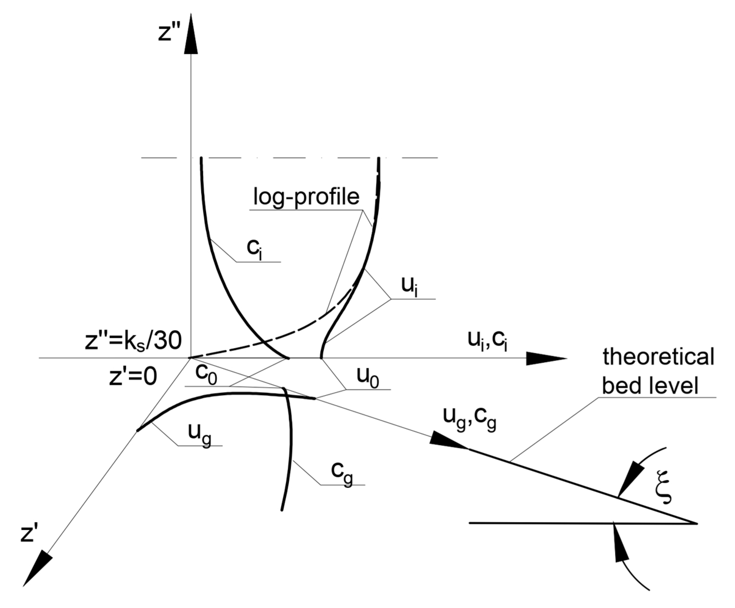

Table 1.
Values of bottom slopes and dimensionless friction for selected measurement series by Damgaard et al. [33] used to verify the model for prediction of vertical sorting of granulometrically heterogeneous sediment.
Table 1.
Values of bottom slopes and dimensionless friction for selected measurement series by Damgaard et al. [33] used to verify the model for prediction of vertical sorting of granulometrically heterogeneous sediment.
| Test 1 | Test 2 | Test 3 | |
|
|
|
|
|
| Test 4 | Test 5 | Test 6 | |
|
|
|
|
|
| Test 7 | Test 8 | Test 9 | |
|
|
|
|
|
| Test 10 | Test 11 | Test 12 | |
|
|
|
|
|
| Test 13 | Test 14 | Test 15 | |
|
|
|
|
Disclaimer/Publisher’s Note: The statements, opinions and data contained in all publications are solely those of the individual author(s) and contributor(s) and not of MDPI and/or the editor(s). MDPI and/or the editor(s) disclaim responsibility for any injury to people or property resulting from any ideas, methods, instructions or products referred to in the content. |
© 2024 by the authors. Licensee MDPI, Basel, Switzerland. This article is an open access article distributed under the terms and conditions of the Creative Commons Attribution (CC BY) license (http://creativecommons.org/licenses/by/4.0/).
Copyright: This open access article is published under a Creative Commons CC BY 4.0 license, which permit the free download, distribution, and reuse, provided that the author and preprint are cited in any reuse.


