
Submitted:
03 June 2024
Posted:
04 June 2024
You are already at the latest version
Abstract
Federated learning is an effective approach for preserving data privacy and security, enabling machine learning to occur in a distributed environment and promoting its development. However, an urgent problem that needs to be addressed is how to encourage active client participation in federated learning. The Shapley Value, a classical concept in cooperative game theory, has been utilized for data valuation in machine learning services. Nevertheless, existing numerical evaluation schemes based on the Shapley Value are impractical as they necessitate additional model training, leading to increased communication overhead. Moreover, participants’ data may exhibit Non-IID characteristics, posing a significant challenge to evaluating participant contributions. Non-IID data weakens the marginal effects of participants, which in turn affects model accuracy and leads to underestimated contribution measurements. Current works often overlook the impact of heterogeneity on model aggregation. This paper presents a fair federated learning contribution measurement scheme that addresses the need for additional model computations. By introducing a noval aggregation weight, it enhances the accuracy of contribution measurement. Experiments on the MNIST dataset show that the proposed method can accurately compute the contributions of participants. Compared to existing baseline algorithms, the model accuracy is significantly improved, with a similar time cost.
Keywords:
Federated Learning
; Shapley Value
; contribution measurement
; Non-IID
1. Introduction
Recent years, with the rapid development of machine learning, there have been great changes in various fields. ML, which is one of the most important areas of Artificial Intelligence, makes it possible to learn a model or a pattern of behavior for a given machine to perform tasks. ML algorithms allow us to process input data using appropriate patterns to generate output data. That is, we can identify and extract patterns from large amounts of data to build learning models [1], serving for predictive modeling and decision-making. In a distributed architecture, it is possible to use consensus mechanisms to manage data consistency [2]. Traditional machine learning methods usually require centralized collection and storage of large-scale data, and then training on a central server or in the cloud. As the public pays increasing attention to data privacy protection, the problem of data silos has become more severe, making the deployment of collective intelligence technology more challenging. Federated Learning (FL), as a new training paradigm for artificial intelligence models dealing with data silos, has gained widespread attention in the past few years [3]. FL extends the training process of machine learning from a single device to multiple devices or compute nodes, enabling parallel processing and model synchronization through the distributed nature of data and computation.This shift can improve training efficiency, scalability and robustness, and provide better solutions in terms of privacy protection.
The performance of the federated learning (FL) system is heavily reliant on sustained participation from local users, high-quality data inputs, and authentic local training. Naturally, not everyone is eager to share their data truthfully without any incentive. Hence, for a viable alliance, all participants should contribute high-quality data and be periodically rewarded accordingly [4]. However, a critical challenge lies in determining a fair compensation mechanism for these local data providers. Effective incentive mechanisms are invaluable in crowdsensing to stimulate the enthusiasm of strategic users [5]. Fairness means rewarding those who provide high-quality data and actively engage in federated learning [6], while punishing participants for bad behavior [7]. A fair return mechanism encourages participants to contribute high-quality data and perform local training in the long run, whereas an unfair allocation scheme may lead to participant misbehavior or permanent withdrawal. Existing federated learning (FL) platforms, such as the Federated AI Technology Enabler (FATE) [8], assume the system already has a stable participant group and does not need to attract more data providers. However, this precondition may not be satisfied in practice, especially when the participants are business organizations. Furthermore, since servers typically have limited knowledge of local users, the global model can be easily poisoned if the server blindly integrates all local models without proper evaluation. Therefore, it is necessary to design a fair contribution measurement method, which also serves as the customer evaluation plan, to quantify the contribution of participants, achieve fair distribution more effectively, and stimulate participants’ enthusiasm.
With the high development of information technology in the era of big data, all kinds of devices generate data, and the generation of data increases exponentially. Mobile devices are the main source of data generation, some of which have spatial characteristics, such as regional mobility, have a high degree of randomness [9]. Assuming that the data has the same probability distribution and is independently distributed (IID) is a classic setup for machine learning. However, this is unrealistic, the composition and properties of things and our daily lives are heterogeneous, non-independent and equally distributed [10]. The problem may be even more pronounced in federated learning. In federated learning (FL), the training data is usually non-independently and identically distributed (Non-IID) across different clients. Existing literature suggests that compared to IID data, the Non-IID data may lead to significantly lower accuracy in federated learning [11].
Non-IID problems exist significantly in federated learning. This issue is due to biased labeling preferences at multiple clients and is a typical setting of data heterogeneity [12]. This means that the number of samples belonging to certain classes in the datasets of different clients may differ. For example, some clients may have a large number of samples belonging to class A, but a small number of samples belonging to class B, while other clients may have the opposite. This kind of dataset heterogeneity is common in federated learning, because different clients usually collect data locally, and these data may have label preferences or specific data collection methods. However, the existing contribution measurement methods of federated learning often ignore the impact of class distribution differences on participant contributions, resulting in inaccurate contribution results.
This paper proposes a more accurate method to measure the contribution of participants in federated learning, which alleviates the influence of data distribution heterogeneity on contribution measurement, thereby improving the accuracy of contribution measurement and encouraging more participants to join federated learning.
The main contributions of this paper are as follows:
- In the process of contribution measurement using Shapley, gradient multiplexing is performed: we use gradient approximation to reconstruct the model, which saves a lot of time. The reconfigurable model can be used to evaluate its performance more easily.
- Considering the heterogeneity of data distribution, a new aggregate weight is used to mitigate the impact of data heterogeneity on contribution measurement and improve the accuracy of contribution measurement.
- We propose a novel metric for measuring participant contributions in federated learning. By utilizing new aggregation weights, this method effectively mitigates the issue of data heterogeneity and enables a fairer assessment of participants’ contribution levels in the federated learning process.
This work is organized as follows: Section 2 describes the relevant background; Section 3 introduces the relevant work; Section 4 describes the formula definition and experimental method in detail; Section 5 describes the main experiments and results; Finally, the conclusions and future work are summarized.
2. Background
This section provides three main backgrounds: Non-IID data, Shapley Value, and Federated learning. The Federated learning approach uses an ML model shared by collaborative learning while protecting user privacy. Non-IID data refers to heterogeneous data with random characteristics. Heterogeneity of category distribution, one of the typical categories in Non-IID, is a common problem in federated learning, which often seen in the inconsistent label distribution among participants. The Shapley Value calculates the contribution of each participant by considering all possible combinations of parties. where the contribution of a party is determined by the expected marginal gain in the value of the data when that party joins the federation [13]. The Shapley Value scheme is intuitive, easy to understand, and ensures a fair assessment of each participant’s individual contribution, and it is widely used in current federated contribution assessment.
2.1. IID and Non-IID Data
By statistical definition, IID means that the random variable data have the same probability distribution and are independent of each other. That is, the data is more homogeneous [14]. In other words, when the samples in the dataset are independent and drawn from the same distribution, we refer to it as IID data. In this case, each sample is sampled independently from the same data distribution. For example, if we have a dataset containing pictures of cats and dogs, and the labels for each sample are evenly distributed (i.e. the same proportion of cats and dogs), then the dataset is IID. In machine learning, it is commonly assumed that the data are independent and identically distributed.
When the samples in the data set do not meet the conditions of independence and the same distribution, we call it Non-IID data. As the training data on each client is collected based on the local environment and usage patterns, there can be significant variations in the size and distribution of the local datasets among different clients [15]. Consequently, the samples in the dataset may exhibit varying distributions or correlations. For instance, let’s consider a dataset used for handwritten digit recognition, where the distribution of samples contributed by different clients may vary.
In federated learning, the IID or Non-IID characteristics of data have a significant impact on the performance of model aggregation and global models. IID data assumes that all clients have the same data distribution, which simplifies and enhances the reliability of model aggregation. Non-IID data, on the other hand, poses significant challenges as the data distribution may vary among different clients. This inconsistency makes model aggregation more difficult, and it can have a notable impact on the performance of the global model.
2.2. Shapley Value
The Shapley Value (SV), named after Lloyd Shapley, is a well-established concept in cooperative game theory that aims to distribute the total profits generated by coalitions of players [16]. The Shapley Value calculates the contribution of each participant to the utility of all possible coalitions they can be a part of, and assigns an unique value to each participant [17], it distributes the benefits among participants by considering all possible ways of cooperative arrangements, ensuring that each partner receives a fair reward based on their individual contributions. In a cooperative game, players can cooperate to generate a payoff. These participants can be individuals, organizations, or any other entity working together. The Shapley Value is designed to address the challenge of fairly distributing rewards in cooperative games.
In cooperative games, multiple participants collaborate to achieve a common goal or generate value. The fundamental concept of the Shapley Value is to quantify the contribution of each participant to the overall outcome, taking into account the order in which participants join the cooperative process. More specifically, the Shapley Value represents the average marginal contribution of each participant towards the final outcome.
Consider a cooperative game involving n players. For a given player i, we consider all possible coalitions that player i can form with other players. The Shapley Value is computed by aggregating the contributions of player i across all possible coalitions and taking a weighted average.
2.3. Federated Learning
The concept of federated learning was first proposed by a research team at Google in 2016. In their research, the team introduced a distributed machine learning approach that enables model training using data scattered across different participating devices while preserving data privacy. The study aimed to address the privacy and security concerns associated with centralized storage of large-scale datasets in traditional centralized machine learning methods. In federated learning, each participant holds their own local data and conducts model training on their respective devices. They then transmit only the updated model parameters to a central server for aggregation. This approach mitigates the challenges associated with centralized storage and transmission of datasets, thereby reducing privacy risks and data transfer costs. Federated learning is extensively employed in various scenarios, including mobile devices, IoT devices, edge servers, etc., to accomplish tasks such as personalized recommendations, speech recognition, image classification, and more. Federated learning, as a novel distributed collaborative learning paradigm, has been widely applied in many scenarios and has successfully trained better models by sharing the private data of multiple clients without leaking privacy [18]. Due to these advantages, federated learning has greatly facilitated data collaboration and sharing among participants, addressing people’s concerns over data privacy.
The FL system enables multiple parties to collaborate on learning tasks while keeping their data local to ensure security. In scenarios where strong privacy is essential, parties may need to be isolated from each other to prevent communication [19]. Federated learning is not merely a component of machine learning but rather a distributed machine learning framework that focuses on a data management process for sharing data among multiple clients while preserving privacy. Figure 1 llustrates the working principle of generic horizontal federated learning:
An illustrative example of federated learning is the word prediction task in the input method of smart devices. While performing this task, it is essential to protect users’ privacy and minimize communication congestion. Rather than transmitting private user data to a central server, training the predictor in a distributed manner is more reasonable. During this task, the smart device engages in periodic communication with the central server to acquire the global model. In each communication epoch, the selected smart device employs its local data for training and transmits the local model to the server. Following model aggregation, the server disseminates the updated global model to other device subsets. The process of continuous iterative training takes place between the server and the participating devices in federated learning until the model converges [20].
Participants establish communication with a trusted central server to exchange relevant information, including models, gradients, and more. Nonetheless, participants acquire this information based on their local data, which may exhibit Non-IID (non-independent and identically distributed) characteristics. Moreover, due to simultaneous communication from multiple parties, there is a potential risk of communication congestion.
3. Related Work
Federated learning is a distributed framework that enables multiple clients to collaborate using their local data to train a shared model while maintaining data privacy and preventing data leakage [21]. In Article [22] the authors present the theoretical concepts of federated learning and apply it to develop a machine learning model using a vehicle’s basic safety information (BSM) dataset. The model is created through the on-board vanet network over the Internet of Vehicles (IoV) to ensure privacy during misconduct detection.
In current deep learning paradigms, local training or the Standalone framework tends to result in over-fitting and thus poor generalizability. This problem can be addressed by Distributed or Federated Learning (FL) that leverages a parameter server to aggregate model updates from individual participants. However, most existing Distributed or FL frameworks have overlooked an important aspect of participation: collaborative fairness [23]. This situation is inherently unfair. In practice, the contribution levels of participants vary for various reasons, such as the quality and quantity of data held by different participants. Federated learning is a collaborative machine learning framework involving multiple participants who maintain their training datasets locally. Evaluating the data contribution of each participant is one of the crucial challenges in federated learning [13]. Implementing a fair measurement method for participant contributions in federated learning ensures fairness among participants, rational resource allocation, establishes a basis for model selection, and encourages active participation in the federated learning process. This helps build a healthy, sustainable federal learning ecosystem.The work by Wang et al. [13] provides a detailed description of the challenges encountered in federated learning and presents common methods for measuring participant contributions, including Leave-one-out and Shapley Value.
Leave-one-out: The Leave-one-out method (LOO) is widely used in machine learning tasks for cross-validation [24]. It is an intuitive data valuation method that measures a data point’s contribution by how much a model’s accuracy will lose after removing it [25]. Based on the idea of LOO, we can use the marginal loss in the value of the participant combination after excluding a certain participant as the contribution of that participant to the federation [26]. Unlike the individual method, the LOO method fully follows the participant combination data value measurement paradigm, that is, the contribution assessment and data value measurement problems are orthogonal. However, the LOO method only considers the marginal benefit brought to the federation by a certain participant when all other participants are fully retained, and this way of specifying the participant to join the federation last to evaluate the contribution also has fairness issues. For example, when there are multiple participants holding the same but highly valuable data for the federation, removing any one of the participants holding that data will not have a significant impact on the federation’s test accuracy, and these participants will be assessed as low-value, but at the same time, removing these participants will greatly reduce the performance of the federation. By eliminating the need for model retraining, this approach improves computation efficiency. Nevertheless, empirical experiments have demonstrated that LOO fails to capture the relative utility between any two samples [27] leading to undervaluation of individual contributions.
Shapley Value: intuitive, easy to understand, to ensure fairness in assessing the individual contributions of each participant, the Shapley Value (SV) is widely employed in current federal contribution assessment. Ghorbani et al. [25] introduce Data Shapley, which applies the concept of Shapley Value (SV) to the data valuation problem. The SV of a data sample represents the average of its marginal contributions to the model, considering all possible joining orders of the samples. Under this approach [25], the authors proposed a truncated Monte Carlo Shapley algorithm, which was implemented through random sampling arrangement and truncation of unnecessary sub-model training and evaluation, thereby reducing unnecessary model evaluations and significantly saving operational resources. Song et al. [6] argue that the existing contribution measurement scheme based on the Shapley Value is not suitable for federated learning due to the additional model training involved, which incurs high costs. In order to solve this problem, the intermediate results of the federated learning training process are used to approximate the reconstruction of the model and reduce the additional model training process. When calculating the Shapley Value, the challenge of permutations is unavoidable. If the number of participants increases significantly, implying a large value of n, it becomes impractical to enumerate all data combinations and compute all marginal contributions precisely. In literature [27], the idea of K-subset is adopted to address this problem. Stratified sampling method is used to randomly select each participant subset of possible size, and the occurrence time of size-K is strictly recorded. And the participant’s Shapley Value is reconstructed to his expected contribution to a K-sized subset with random cardinality. Wei et al. [28] introduced a Truncated Multi-Round (TMR) method in their paper, which is an improvement over the MR algorithm. It considers the accuracy of each round, and assigns higher weights to training rounds with higher accuracy when performing the weighted averaging. It uses a decay factor to ignore the weights of the round-level in the last few rounds, and only constructs and evaluates the models that have an effective influence on the final result.
Although federated learning (FL) offers an appealing framework for addressing the ’data silos’ challenge and decomposing a machine learning task into a collaborative effort, it faces several practical obstacles. On one hand, existing studies make the optimistic assumption that all mobile devices unconditionally contribute their resources [29]. However, this assumption is unrealistic and unfair to the parties involved. On the other hand, concerning training effectiveness, data distributed among different local participants are often non-independent and non-identically distributed (Non-IID) [30]. Zhu et al. [31] believe that the presence of Non-IID data inevitably results in a decline in FL accuracy, primarily due to the bias introduced by Non-IID data into local model weights. The presence of heterogeneous data affects the convergence speed and learning ability of the model. Lyu et al. [32] introduced the Federal Average (FedAvg) model, a practical approach for joint learning of deep networks based on iterative averaging. FedAvg is frequently employed as an aggregation model, known for its robustness to Non-IID data.
4. Materials and Methods
In current common contribution evaluation schemes, assessing individual utility through model output changes often requires multiple ML model retrainings, which can be time-consuming for deep neural networks and pose challenges for aggregation servers. The server must allocate additional computing resources for model retraining, which in turn impacts the model’s convergence speed. Currently, the widely adopted algorithm for global model updates on the server is the FedAvg algorithm [33]. FedAvg, which performs weighted averaging based on the data volume from participants, is a common and effective method in federated learning. However, according to the Pareto principle, especially in cases of data heterogeneity, using only the one-dimensional data volume to obtain the aggregated global model is often insufficient [34]. The heterogeneity in data distribution not only affects the model’s accuracy but also impacts the evaluation of participants’ contributions. To solve these problems, we propose a fair contribution measurement scheme based on the Shapley Value. By circumventing the need for additional submodel retraining, our proposed scheme also mitigates the adverse effects of data distribution heterogeneity.
4.1. Contribution Measurement Method based on Shapley Value
As an example of horizontal federated learning, which we show in Figure 1, suppose N= clients participating in federated learning have local private data sets , i∈. Suppose that federated learning requires T iterations to achieve a convergent model. In each epoch t∈, participant i downloads the global model from the server. It utilizes its local data for model training, resulting in a local model . Subsequently, participant i sends the updated submodel to the server, which calculates the corresponding gradient based on the uploaded submodel:
On the server side, it will collect each submodel, calculate the update gradient of the corresponding participant, store it, and then perform an aggregation operation, which is the FedAvg algorithm in literature [29] to update the global model. Its specific operations are as follows:
Where is the size of training data of participant i and is the sum of data owned by all participants.
Data Shapley Value [25], (N,U), can be used to evaluate the contribution by each participant.It is defined as:
Here, U represents a utility evaluation function that measures the predictive performance of the learned model on an independent test set. In this paper, model accuracy is employed as the evaluation metric. The function is executed on the server, leveraging its higher computing power to efficiently obtain results without impacting the model’s runtime. The Shapley Value is attractive for contribution evaluation problems because it satisfies some desirable axiomatic properties. We summarize the following common axioms [35]:
- Group Rationality: The value of the entire dataset is completely distributed among all users, i.e. .
- Fairness: (1) Two users who are identical with respect to what they contribute to a dataset’s utility should have the same value. That is, if user i and j are equivalent in the sense that: i.e., if , then i=j; (2) Users with zero marginal contributions to all subsets of the dataset receive zero payof: i.e., if , then i=0 for all .
- Additivity: The values under multiple utilities sum up to the value under a utility that is the sum of all these utilities: i.e., where are two utility tests.
4.2. Gradient-Based Model Reconstruction
During the evaluation of , this section involves additional submodel reconstruction. To address this issue, we employ a gradient-based approach to reconstruct the submodel in federated learning (FL): Suppose that in epoch t, we need to reconstruct the submodel for performance evaluation, which can be defined as follows:
By performing this step, the server can evaluate the submodel without the need for retraining, thereby significantly reducing computational resources and accelerating the model’s convergence.
4.3. Build a new aggregate weight
Currently, the commonly used algorithm for updating the global model on the server is the FedAvg algorithm [29]. However, this algorithm may have certain limitations. During the aggregate weight calculation process, the algorithm assigns weights solely based on the data set sizes, neglecting the impact of data distribution heterogeneity. The presence of heterogeneous data weakens the contribution level of participants to the global model, which makes the results of contribution measurement inaccurate. To alleviate this issue, previous studies have mainly focused on regularization techniques for local models or fine-tuning the global model, overlooking the adjustment of aggregation weights, often assigning weights solely based on dataset sizes [12]. Considering the impact of data distribution heterogeneity on the model, it may be more reasonable to incorporate it into the calculation of aggregate weights in order to mitigate its effects.
Hence, our approach involves quantifying the issue of data distribution heterogeneity and incorporating it into the computation of updated aggregate weights. Firstly, we assume a global category distribution on the server: A global category distribution is defined as one where each data category is evenly distributed, and the number of categories is consistent. This assumption promotes fairness among categories and enhances the generalization ability of the global model. Based on this assumption, we can calculate the local category distribution for each participant. The participants upload their respective local category distributions along with their local models during the global model aggregation phase. Subsequently, we can readily calculate the discrepancy between each participant’s distribution and the global distribution on the server side, denoted as . In this study, we employ the Kullback-Leibler (KL) divergence to quantify the difference between these distributions:
According to formula (2), the weight of the size of the dataset in the formula is defined as . That is to say: . Using the previously calculated data distribution difference value for each participant, we can incorporate it into formula (2) to obtain a new aggregate weight, denoted as :
Here, k=i, a and b represent two constants. By utilizing equation (6), we establish a relationship between the aggregate weights and the dataset size as well as the distribution of participant categories . By formulating the aggregate weights, we can assign smaller weights to participants with higher difference levels, thereby mitigating the impact of heterogeneous data on the model. This approach aims to enhance the accuracy of contribution measurement.
4.4. New Aggregate Function
Based on the preceding research, we can redefine formula (2) by incorporating formula (6) with the new aggregate weights, thus determining our final aggregate function.
Based on the aforementioned modifications, we have established the model structure of this paper, which is illustrated in Figure 2:
During the process of model aggregation, participants upload not only their local models but also the local category distribution in the local information upload stage. The server calculates the new aggregate weight based on the and updates the global model, which is subsequently distributed to the participants.
4.5. Contribution Measurement Algorithm based on Shapley Value
The core idea of our algorithm is that in each epoch, the server collects local models from different participants, uses them to calculate the relevant gradient information, and uses the gradient information to approximately reconstruct the model on different data set combinations, avoiding additional training. Next, we use formula (3) to evaluate the performance of these reconstructed models and further evaluate the contribution level of each participant. Ultimately, we obtain the final result by taking a weighted average of values from different training epochs. See the pseudo-code description for details. Our algorithm is divided into two parts. Lines 1-23 depict the server-side execution. More specifically, Lines 1-14 illustrate the calculation process for the global model: In the first epoch of model training, participants first calculate the local category distribution information (only in the first epoch of calculation), at the same time use the local data to conduct local training on the initial model sent by the server, and upload the trained local model and local category distribution information to the server. Upon receiving the information, the server independently calculates the model gradient for each participant, and the gradient information is stored with the cycle information, and the difference between the local distribution and the global distribution of each participant is calculated. Then, the aggregate weights with distribution differences proposed above are calculated and used to update the global model. In lines 15-20, leveraging formula (3) and the reconstructed model from each epochs, we estimate , representing the contribution index of participant i in epoch t+1. In line 22, we use the attenuation factor ∈(0,1) to regulate the calculation of the final SV. The purpose is that when calculating the global SV, it is gradually affected by the common influence of all data sets due to increasing iteration epochs. Therefore, earlier epochs are given a higher weight. Part 24-32, the second segment, is executed by the client: The client receives a global model from the server, trains the local model with local data using gradient descent algorithms, and subsequently transfers the trained local model to a trusted server.
|
Algorithm 1: FL Participant Contribution Evaluation
|
|
Input: B is the local minibatch size, E is the number of local epochs, and is the learning rate, is the global distribution we set.
Server executes:
|
5. Experiment and Result
In this section, we perform experiments on the aforementioned algorithms under various data distributions to assess their performance and compare them against existing mainstream methods.
5.1. Dataset
The experiment was conducted on the MNIST dataset [36], which comprises a collection of handwritten digit images consisting of over 60,000 training images and 10,000+ test images. We randomly sampled 5,421 images for each digit category, resulting in a total of 54,210 samples for the experiment. Additionally, we randomly selected 8,920 images for each digit as a separate test dataset, resulting in a total of 89,200 samples utilized for testing. For the FL experiment, we established five clients. To assess the performance of the proposed algorithm under various FL settings, we partitioned the training set into five distinct cases:
- Same Distribution and Same Size: In this setup, we randomly partitioned the dataset into five equally sized subsets, each containing the same number of images and maintaining the same label distribution.
- Same Distribution and Different Size: We randomly sampled from the training set according to predetermined proportions to create a local dataset for each participant. We ensured that each participant has an equal number of images for each digit category. Participant 1 had a proportion of 2/20; Participant 2 had a proportion of 3/20; Participant 3 had a proportion of 4/20; Participant 4 had a proportion of 5/20; and Participant 5 had a proportion of 6/20.
- Different Distributions and Same Size: In this setup, we divide the dataset into five equal parts, with each part having a distinct distribution of feature data. To be specific, the dataset for participant 1 comprises 80% of the samples labeled as ’1’ and ’2’, while the remaining 20% of the samples are equally distributed among the other numbers. This distribution strategy also applies to participants 2, 3, and 4. The final client exclusively contains handwritten numeric samples labeled as ’8’ and ’9’.
- Biased and unbiased: This method builds upon the ’Different Distributions and Same Size’ method by aiming to enhance the heterogeneity of data distributions among clients. Under the condition that each participant possesses an equal number of samples, the method employs a more heterogeneous setup. It includes four biased clients, each containing two categories of non-overlapping data, and one unbiased client with an equal number of samples from all ten categories.
- Noisy Labels and Same Size: The data partitioning in this setting is identical to that in the ’Same Distribution and Same Size’ method. Subsequently, varying proportions of Gaussian noise are introduced to the input images. The specific configuration is as follows: participant 1 has 0% Gaussian noise ; participant 2 has 5% ; participants 3 have 10% ; participant 4 has 15% ; and participant 5 has 20%.
5.2. Baseline Algorithm
Although there are many federated learning contribution measurement schemes based on Shapley Value, they often involve additional model evaluation and affect model convergence. Therefore, we selected the widely used and classic contribution measurement scheme as the baseline algorithm. These schemes employ measures to reduce the need for additional model evaluation, and our work is more appropriate in comparison with these schemes. Here’s the algorithm we used to make the comparison:
- Exact Shapley : This is the exact computation method proposed in literature[25]. This method calculates the original Shapley Values according to formula (3), which involves a large amount of sub-model reconstruction. It evaluates all possible combinations of participants, and each submodel is trained using their respective datasets.
- TMC Shapley: In this approach [25], models of a subset of FL participants are trained using their local datasets and the initial FL model. Mont-carlo’s Shapley Value estimation is performed by randomly sampling permutations and truncating unnecessary submodel training and evaluation.
- K-subset Shapley: This method [27] randomly takes every possible size subset of a participant, strictly records the occurrence time of size K, and reconstructs the participant’s Shapley Value to his expected contribution to a K-size subset with a random base. The way retains the hierarchical structure of Shapley Value, it has high approximation precision.
- SMR Shapley: Similar to the MR method in the literature [6], gradients are utilized to update subsets of the global model, thereby avoiding the need for local users to retrain and conserving computational resources. The Shapley Value of each participant is calculated in each training epoch, and the results are recorded. The sum of these contributions is aggregated to reflect the overall performance of each client across the federated training process.
- TMR Shapley: The method is the Truncated Multi-Round (TMR) construction introduced in [28], which is an improvement of the MR algorithm. It uses a decay factor and the accuracy of each round to control the weights of the round-level in the final result. Once the round-level become negligible for the final result, the model is no longer constructed or evaluated.
5.3. Performance Evaluation Metrics.
The performance of the comparison approaches is evaluated with the following metrics:
Time: We compared the training time of the model with the time required to calculate the contribution index.
SV: We compare the Shapley Value of the participants obtained using different algorithms in various scenarios.
Accuracy: We evaluated the model accuracy using different algorithms in various scenarios.
5.4. Experimental Result
In this section, we analyze the results of the experiment conducted in the aforementioned five settings:
Same Distribution and Same size: In this case, each participant is assigned to the same data category and quantity. Thus, the expected outcome is for each participant to have the same SV. Figure 3 illustrates the variations of different algorithms with respect to the number of training epochs in this scenario. As observed in Figure 3 (a), (c) and (d) , the performance of ’Exact Shapley’, ’k-subset Shapley’, and ’SMR Shapley’ methods is not optimal, resulting in significant variation in SV among the five participants. Figure 3 (b), (e) and (f) demonstrate that while the ’TMC Shapley’ and ’TMR Shapley’ algorithms has achieved the desired outcome with relatively close SV among multiple participants, its performance is still inferior to our algorithm. The results obtained from our algorithm indicate that the SV of the five participants are very close to each other. Regarding time and accuracy, Table 1 reveals that the ’Exact Shapley’ method exhibits low efficiency, requiring substantial time, and yields subpar model accuracy. ’TMR Shapley’ algorithm takes the least time, but its model accuracy is lower than ours. Our method attains favorable outcomes while maintaining comparable runtime to other baseline algorithms.
Same Distribution and Different size: In this setting, we make the feature distribution of the participants consistent and change the number of their features. As can be seen from Figure 4 (a), (b), (c), (d) and (e), the baseline algorithms are ill-suited for this Non-IID scenario, resulting in suboptimal experimental outcomes. When the last participant possesses the most feature data, their contribution should far exceed that of other participants. Furthermore, the SV of the first four participants exhibit a decreasing trend, contrary to the actual results. Figure 4 (f) demonstrates that our algorithm effectively captures this characteristic, yielding precise measurement results. Our algorithm accurately determines that the participant (Participant 5) with the highest number of feature data has a positive and maximum SV. And it correctly captures the increasing trend of the SV among the first four participants, unlike the unreasonable measurement results of the baseline algorithm. In terms of time and accuracy, we can see from Table 2 that although our time cost is not optimal, it is still within the acceptable range, but compared with other baseline algorithms, we have higher accuracy. Compared with the ’Exact Shapley’ algorithm, the algorithm time is greatly saved.
Different Distributions and Same Size: In this setting, each participant is allocated the same data quantity, but their feature distributions are heterogeneous. First,let’s look at the SV measurement. As depicted in Figure 5 (a), (b), (c), (d) and (e), the following observations can be made: Among the compared baseline algorithms, none of them exhibit robustness against the heterogeneity of the data distribution. Specifically, when participant 5’s data exhibits high heterogeneity, the baseline method yields a negative SV for that participant. However, this result contradicts the definition of SV. Participants who contribute high-quality data through realistic training should be assigned larger SV, while those providing random data should receive smaller SV [37]. The presence of heterogeneous data adversely affects the accuracy of SV measurements. Our algorithm alleviates the impact of heterogeneous data and accurately assigns a positive SV to participant 5, as evident from Figure 5 (f). In contrast to the baseline algorithm, our algorithm achieves accurate measurement of the SV for each participant. As evident from Table 3, the ’Exact Shapley’ method remains computationally expensive. Although the time of ’TMR Shapley’ algorithm is shorter, the model accuracy is not as good as ours. Our algorithm achieves better results when the time overhead is similar to other baseline algorithms.
Biased and Unbiased: This setting is similar to the ’Different Distributions and Same Size’ scenario, but it exhibits a greater degree of heterogeneity in feature distribution. Figure 6 provides additional evidence of our algorithm’s robustness in handling data distribution heterogeneity. While all the algorithms measured a higher contribution from the last unbiased participant, the outcomes for the remaining four biased participants were unsatisfactory. Figure 6(b), (c), (d) and (e) demonstrate that the SV of the four biased participants, as measured by the ’TMC Shapley’, ’K-subset Shapley’ ’SMR Shapley’, and ’TMR Shapley’ methods, are negative. Figure 6 (a) and (f) illustrate that the ’Exact Shapley’ method assigns a positive SV to participant 5, but exhibits significant discrepancies in SV measurements for the four biased participants. Our algorithm accurately captures the larger SV of the unbiased participant while assigning the smaller positive SV to the remaining four biased participants who have no harmful data, and achieves subtle numerical differences between the biased participants. This is consistent with expectations and improves accuracy compared to the baseline algorithm. Table 4 highlights that the ’Exact Shapley’ method incurs the highest time overhead and ’TMR Shapley’ algorithm still has the best time overhead. Our algorithm exhibits comparable time requirements to other baseline algorithms, while achieving superior accuracy in this scenario.
Noise labels and Same size: Next, we investigate the impact of noise labels, as illustrated in Figure 7. Figure 7 (b), (c), (d), (e) and (f) demonstrate the robustness of our algorithm and the baseline algorithms (’TMC Shapley’, ’K-subset Shapley’, ’SMR Shapley’ and ’TMR Shapley’) to noisy data. Specifically, the SV of the last four participants with noisy data exhibits the expected decreasing trend, distinctly differing from the SV of the first participants with noiseless data. The SV of the last four noisy players is much smaller than the SV of the first noiseless player. However, in the case of the ’Exact Shapley’ algorithm, Figure 7 (a) reveals that the SV of the last four participants with noisy data do not show the expected decreasing trend, and the SV of Participant 1 without noise is smaller than that of participants with noisy data. Consequently, the results are evidently inaccurate. Regarding time and accuracy, Table 5 indicates that the ’Exact Shapley’ algorithm incurs significant time overhead without achieving high model accuracy. Our algorithm achieves model accuracy comparable to other baselines, and although the time overhead is not optimal, it is still within the acceptable range.
6. Conclusions
This paper proposes a fair contribution evaluation method based on the Shapley Value, addressing the limitations of existing Federated Learning (FL) contribution evaluation methods. The proposed method assesses participants’ contributions to FL model performance based on the Shapley Value, without requiring additional model training or exposing sensitive local data. Its key idea involves reconstructing the model using gradients. Additionally, we utilize a novel aggregation function to address the issue of data distribution heterogeneity, thereby mitigating its impact on the measurement of contributions. Extensive experiments were conducted on the MNIST dataset, demonstrating that our method accurately measures participant contributions and exhibits robustness for Non-IID data. Our method achieves comparable speed and higher accuracy compared to other baseline approaches.
However, the algorithm’s performance is suboptimal when dealing with noisy label data. In future work, attention mechanisms could be incorporated to enable the model to selectively attend to the noiseless components, thereby mitigating the impact of noisy labels. Furthermore, this method holds potential for extension to the domain of federated medical image segmentation, aiming to enhance the accuracy of segmentation.
Author Contributions
Conceptualization, G.P. and Y.Y.; methodology, G.P. and Y.Y.; validation, G.P.; writing—original draft preparation, G.P.; writing—review and editing, Y.Y. and W.G.; supervision, Y.Y. and Y.S.; project administration, Y.S. All authors have read and agreed to the published version of the manuscript
Funding
the Natural Science Project of Xinjiang University Scientific Research Program (XJEDU2021Y0 03) and Xinjiang Tianchi Talent Youth Doctoral Program (2023xjtcyc) .
Institutional Review Board Statement
Not applicable.
Informed Consent Statement
Not applicable.
Data Availability Statement
Data are contained within the article.
Acknowledgments
Not applicable.
Conflicts of Interest
The authors declare no conflict of interest.
References
- Simeone, O. A very brief introduction to machine learning with applications to communication systems. IEEE Transactions on Cognitive Communications and Networking 2018, 4, 648–664. [Google Scholar] [CrossRef]
- Qu, Z.; Zhang, Z.; Liu, B.; Tiwari, P.; Ning, X.; Muhammad, K. Quantum detectable Byzantine agreement for distributed data trust management in blockchain. Information Sciences 2023, 637, 118909. [Google Scholar] [CrossRef]
- Yang, C.; Liu, J.; Sun, H.; Li, T.; Li, Z. WTDP-Shapley: Efficient and effective incentive mechanism in federated learning for intelligent safety inspection. IEEE Transactions on Big Data 2022. [Google Scholar] [CrossRef]
- Yang, Q.; Liu, Y.; Chen, T.; Tong, Y. Federated machine learning: Concept and applications. ACM Transactions on Intelligent Systems and Technology (TIST) 2019, 10, 1–19. [Google Scholar]
- Lu, J.; Liu, H.; Jia, R.; Zhang, Z.; Wang, X.; Wang, J. Incentivizing proportional fairness for multi-task allocation in crowdsensing. IEEE Transactions on Services Computing 2023. [Google Scholar] [CrossRef]
- Song, T.; Tong, Y.; Wei, S. Profit allocation for federated learning. 2019 IEEE International Conference on Big Data (Big Data). IEEE, 2019, pp. 2577–2586.
- Hussain, G.J.; Manoj, G. Federated learning: A survey of a new approach to machine learning. 2022 First International Conference on Electrical, Electronics, Information and Communication Technologies (ICEEICT). IEEE, 2022, pp. 1–8.
- FedAI. Online. Available at https://www.fedai.org.
- Xiao, Z.; Fang, H.; Jiang, H.; Bai, J.; Havyarimana, V.; Chen, H.; Jiao, L. Understanding private car aggregation effect via spatio-temporal analysis of trajectory data. IEEE transactions on cybernetics 2021, 53, 2346–2357. [Google Scholar] [CrossRef]
- Hellström, H.; da Silva Jr, J.M.B.; Amiri, M.M.; Chen, M.; Fodor, V.; Poor, H.V.; Fischione, C.; others. Wireless for machine learning: A survey. Foundations and Trends® in Signal Processing 2022, 15, 290–399. [Google Scholar] [CrossRef]
- Wang, S.; Zhao, H.; Wen, W.; Xia, W.; Wang, B.; Zhu, H. Contract Theory Based Incentive Mechanism for Clustered Vehicular Federated Learning. IEEE Transactions on Intelligent Transportation Systems 2024. [Google Scholar] [CrossRef]
- Ye, R.; Xu, M.; Wang, J.; Xu, C.; Chen, S.; Wang, Y. Feddisco: Federated learning with discrepancy-aware collaboration. International Conference on Machine Learning. PMLR, 2023, pp. 39879–39902.
- Yong, W.; Guoliang, L.; Kaiyu, L. Survey on contribution evaluation for federated learning. Journal of Software 2022, 34, 1168–1192. [Google Scholar]
- Clauset, A. Inference, models and simulation for complex systems. Lecture Notes CSCI 2011, 70001003. [Google Scholar]
- Sattler, F.; Wiedemann, S.; Müller, K.R.; Samek, W. Robust and communication-efficient federated learning from non-iid data. IEEE transactions on neural networks and learning systems 2019, 31, 3400–3413. [Google Scholar] [CrossRef]
- Shapley, L. A value for n-person games. <italic>Classics in Game Theory</italic> <bold>2020</bold>, pp. 69–79.
- Liu, Z.; Chen, Y.; Yu, H.; Liu, Y.; Cui, L. Gtg-shapley: Efficient and accurate participant contribution evaluation in federated learning. ACM Transactions on Intelligent Systems and Technology (TIST) 2022, 13, 1–21. [Google Scholar] [CrossRef]
- Zhu, H.; Li, Z.; Zhong, D.; Li, C.; Yuan, Y. Shapley-value-based Contribution Evaluation in Federated Learning: A Survey. 2023 IEEE 3rd International Conference on Digital Twins and Parallel Intelligence (DTPI). IEEE, 2023, pp. 1–5.
- Verbraeken, J.; Wolting, M.; Katzy, J.; Kloppenburg, J.; Verbelen, T.; Rellermeyer, J.S. A survey on distributed machine learning. Acm computing surveys (csur) 2020, 53, 1–33. [Google Scholar] [CrossRef]
- Li, T.; Sahu, A.K.; Talwalkar, A.; Smith, V. Federated learning: Challenges, methods, and future directions. IEEE signal processing magazine 2020, 37, 50–60. [Google Scholar] [CrossRef]
- Learning, F. Collaborative machine learning without centralized training data. Publication date: Thursday, April 2017, 6. [Google Scholar]
- Uprety, A.; Rawat, D.B.; Li, J. Privacy preserving misbehavior detection in IoV using federated machine learning. 2021 IEEE 18th annual consumer communications & networking conference (CCNC). IEEE, 2021, pp. 1–6.
- Lyu, L.; Xu, X.; Wang, Q.; Yu, H. Collaborative fairness in federated learning. <italic>Federated Learning: Privacy and Incentive</italic> <bold>2020</bold>, pp. 189–204.
- Kearns, M.; Ron, D. Algorithmic stability and sanity-check bounds for leave-one-out cross-validation. Proceedings of the tenth annual conference on Computational learning theory, 1997, pp. 152–162.
- Ghorbani, A.; Zou, J. Data shapley: Equitable valuation of data for machine learning. International conference on machine learning. PMLR, 2019, pp. 2242–2251.
- Wang, G.; Dang, C.X.; Zhou, Z. Measure contribution of participants in federated learning. 2019 IEEE international conference on big data (Big Data). IEEE, 2019, pp. 2597–2604.
- Jia, R.; Dao, D.; Wang, B.; Hubis, F.A.; Hynes, N.; Gürel, N.M.; Li, B.; Zhang, C.; Song, D.; Spanos, C.J. Towards efficient data valuation based on the shapley value. The 22nd International Conference on Artificial Intelligence and Statistics. PMLR, 2019, pp. 1167–1176.
- Wei, S.; Tong, Y.; Zhou, Z.; Song, T. Efficient and Fair Data Valuation for Horizontal Federated Learning. Cham: Springer International Publishing, 2020, <italic>10</italic>, 139–152. [CrossRef]
- Kang, J.; Xiong, Z.; Niyato, D.; Xie, S.; Zhang, J. Incentive mechanism for reliable federated learning: A joint optimization approach to combining reputation and contract theory. IEEE Internet of Things Journal 2019, 6, 10700–10714. [Google Scholar] [CrossRef]
- Kang, J.; Xiong, Z.; Niyato, D.; Zou, Y.; Zhang, Y.; Guizani, M. Reliable federated learning for mobile networks. IEEE Wireless Communications 2020, 27, 72–80. [Google Scholar] [CrossRef]
- Zhu, H.; Xu, J.; Liu, S.; Jin, Y. Federated learning on non-IID data: A survey. Neurocomputing 2021, 465, 371–390. [Google Scholar] [CrossRef]
- McMahan, B.; Moore, E.; Ramage, D.; Hampson, S.; y Arcas, B.A. Communication-efficient learning of deep networks from decentralized data. Artificial intelligence and statistics. PMLR, 2017, pp. 1273–1282.
- Castro, J.; Gómez, D.; Tejada, J. Polynomial calculation of the Shapley value based on sampling. Computers & Operations Research 2009, 36, 1726–1730. [Google Scholar]
- Yang, C.; Hou, Z.; Guo, S.; Chen, H.; Li, Z. SWATM: Contribution-Aware Adaptive Federated Learning Framework Based on Augmented Shapley Values. 2023 IEEE International Conference on Multimedia and Expo (ICME). IEEE, 2023, pp. 672–677.
- Dong, L.; Liu, Z.; Zhang, K.; Yassine, A.; Hossain, M.S. Affordable federated edge learning framework via efficient Shapley value estimation. Future Generation Computer Systems 2023, 147, 339–349. [Google Scholar] [CrossRef]
- LeCun, Y.; Cortes, C.; Burges, C. MNIST handwritten digit database. ATT Labs [Online]. Available: http://yann.lecun.com/exdb/mnist 2010, 2. [Google Scholar]
- Zhang, J.; Guo, S.; Qu, Z.; Zeng, D.; Zhan, Y.; Liu, Q.; Akerkar, R. Adaptive federated learning on non-iid data with resource constraint. IEEE Transactions on Computers 2021, 71, 1655–1667. [Google Scholar] [CrossRef]
Figure 1.
General Federated Learning Structure Diagram.
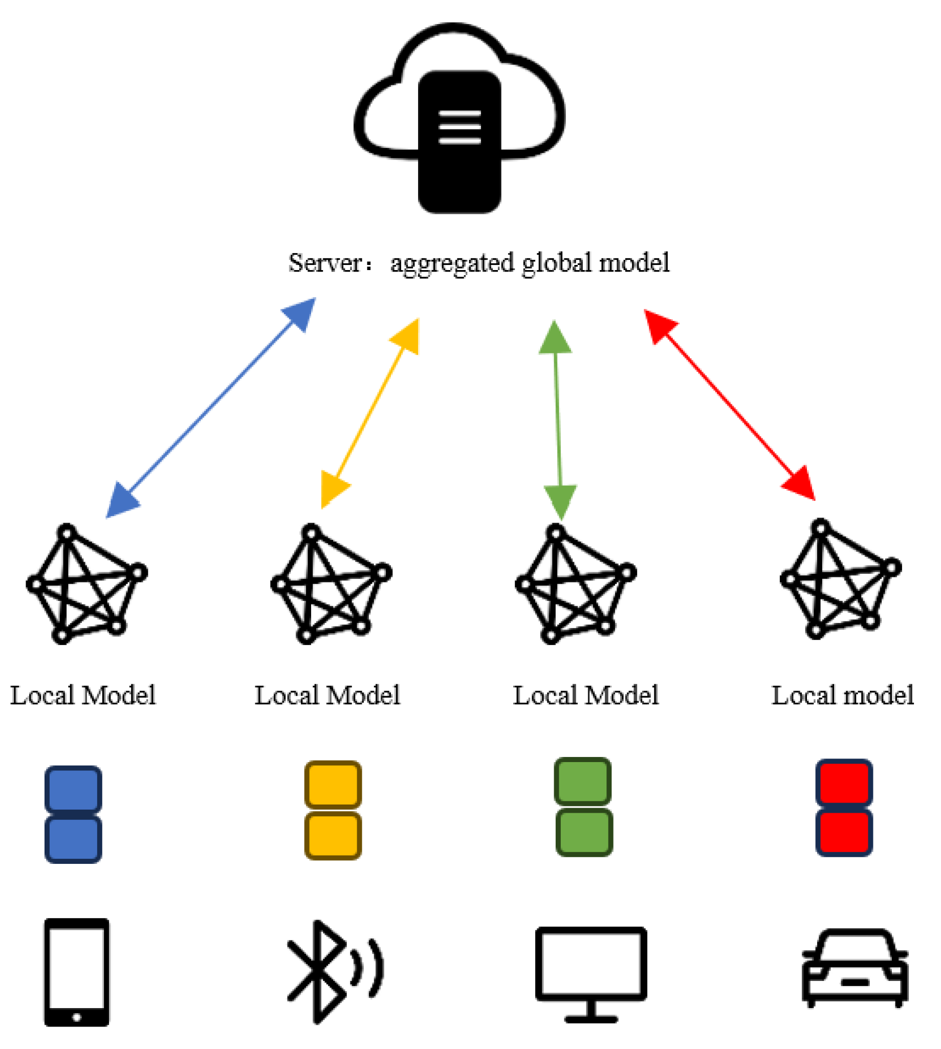
Figure 2.
Modified federated learning structure diagram.
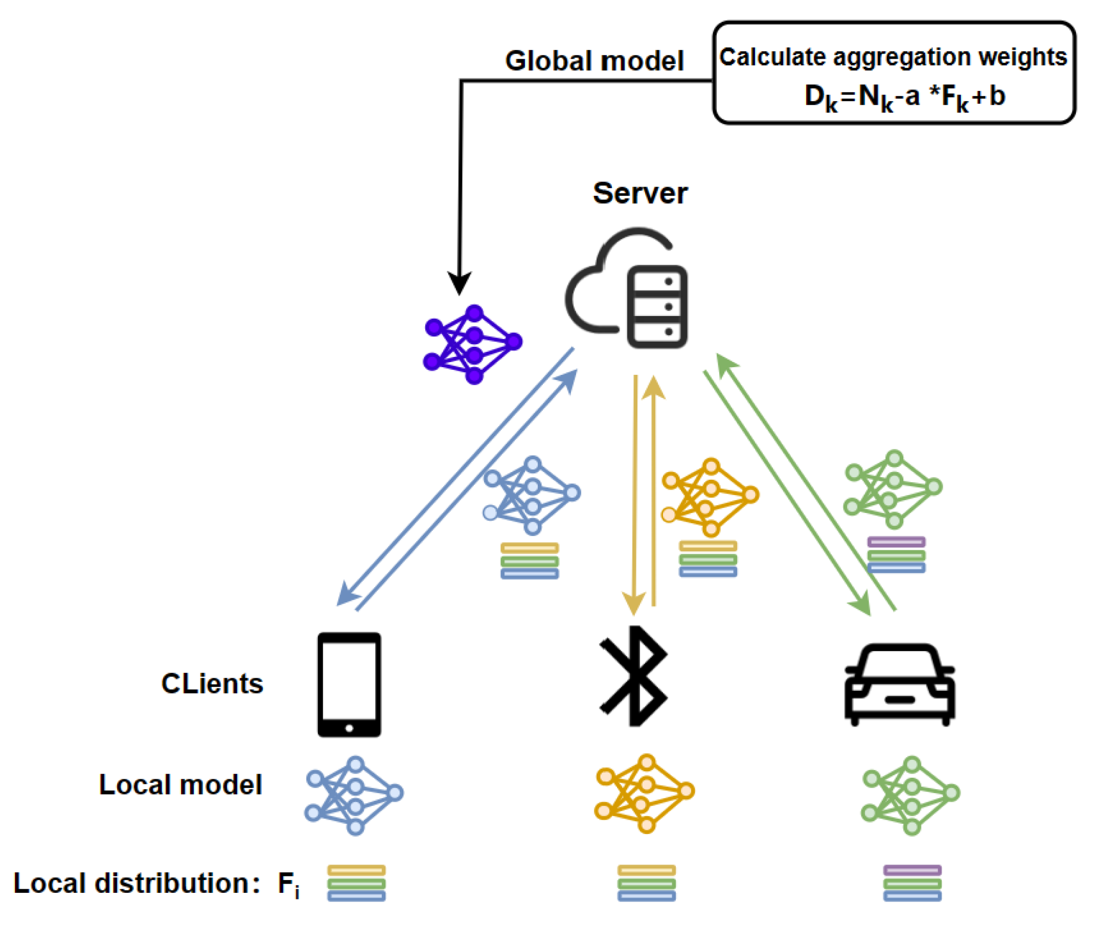
Figure 3.
Same Distribution and Same size
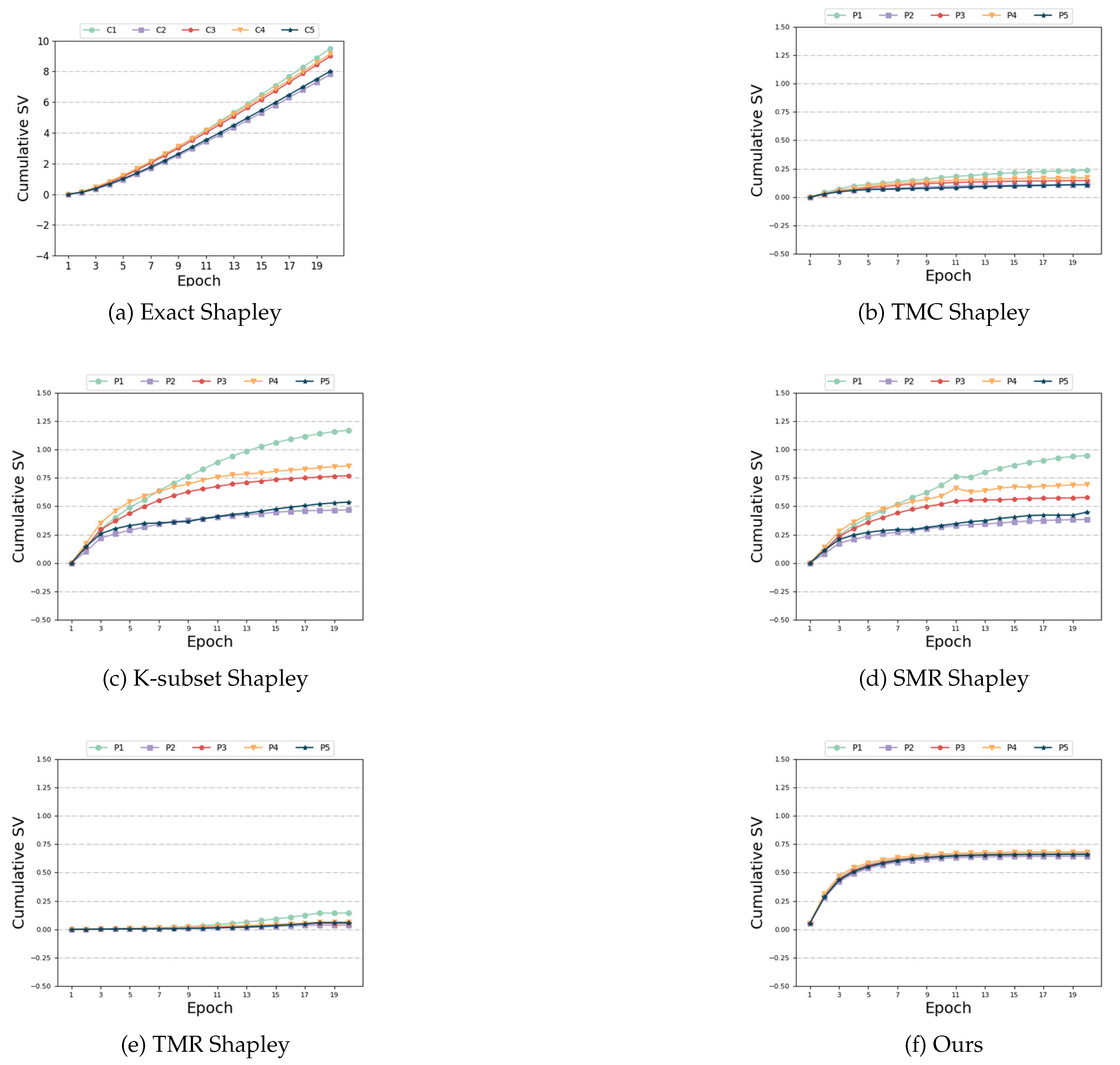
Figure 4.
Same Distribution and Different size
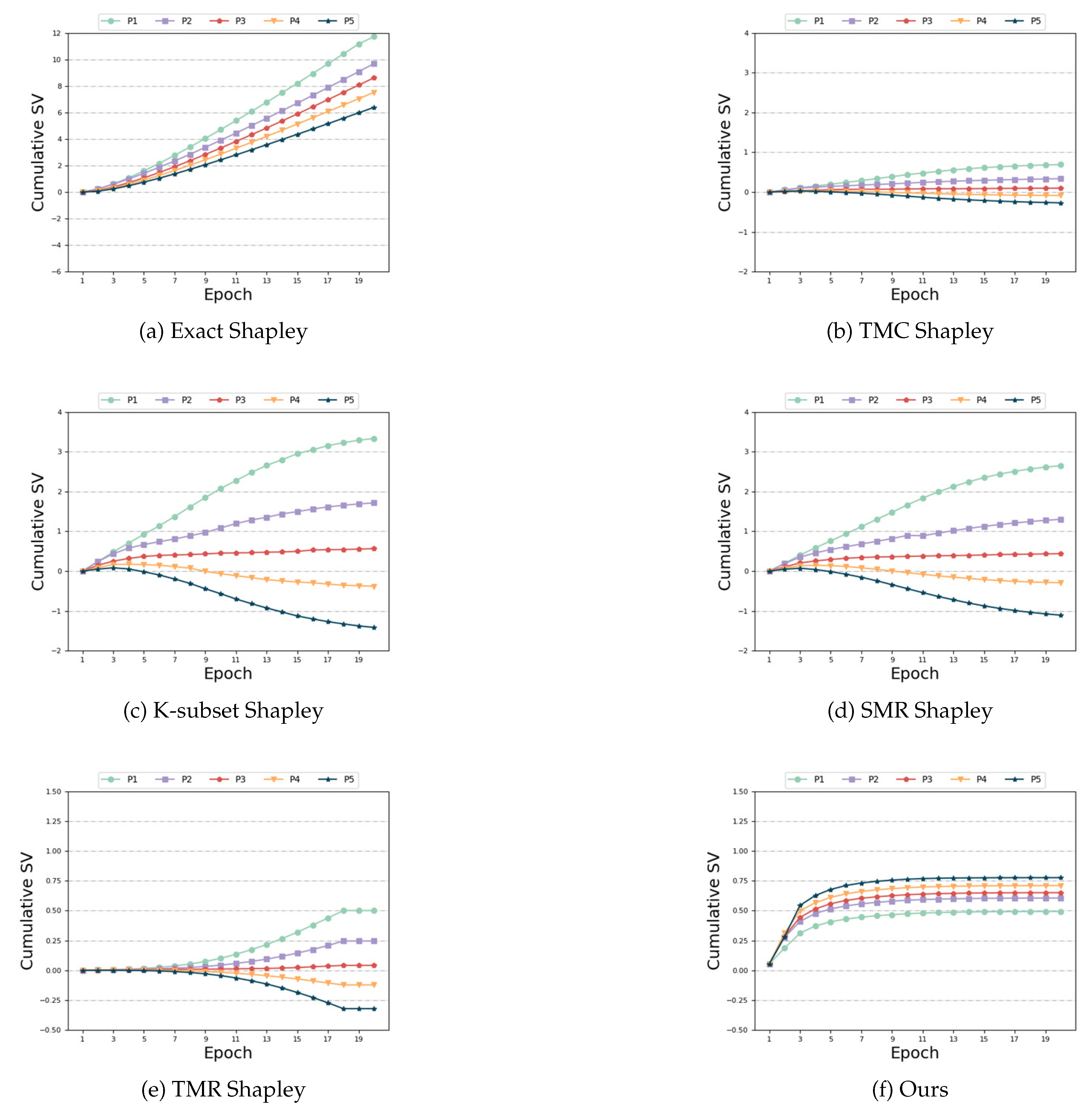
Figure 5.
Different Distributions and Same Size
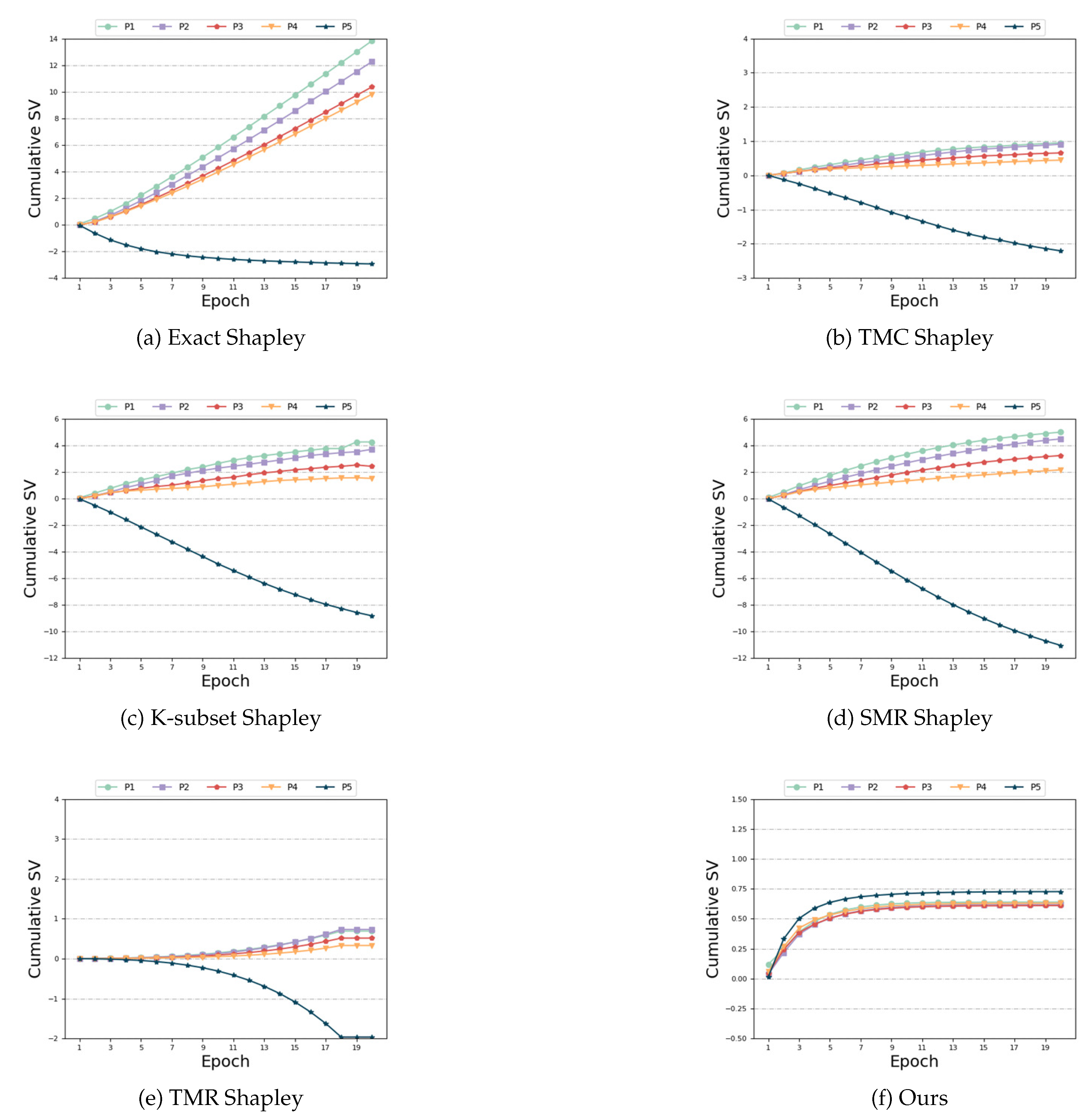
Figure 6.
Biased and Unbiased
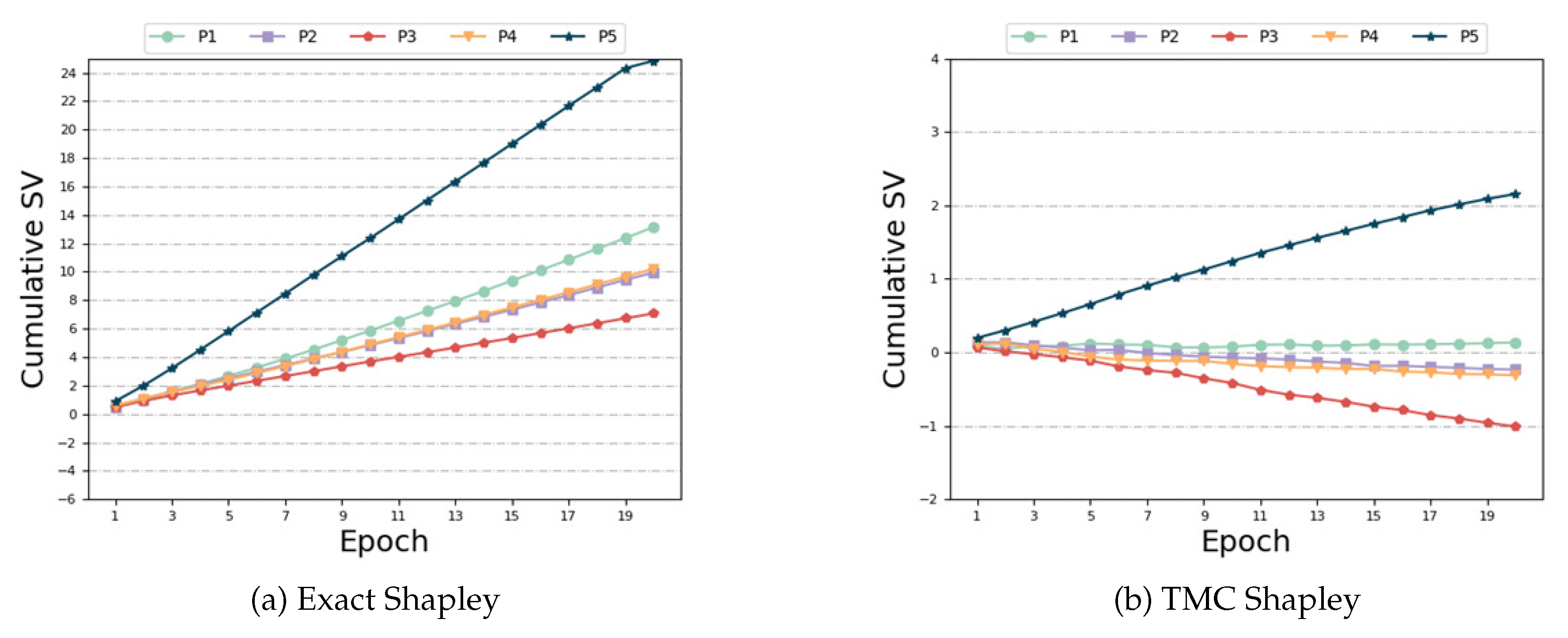
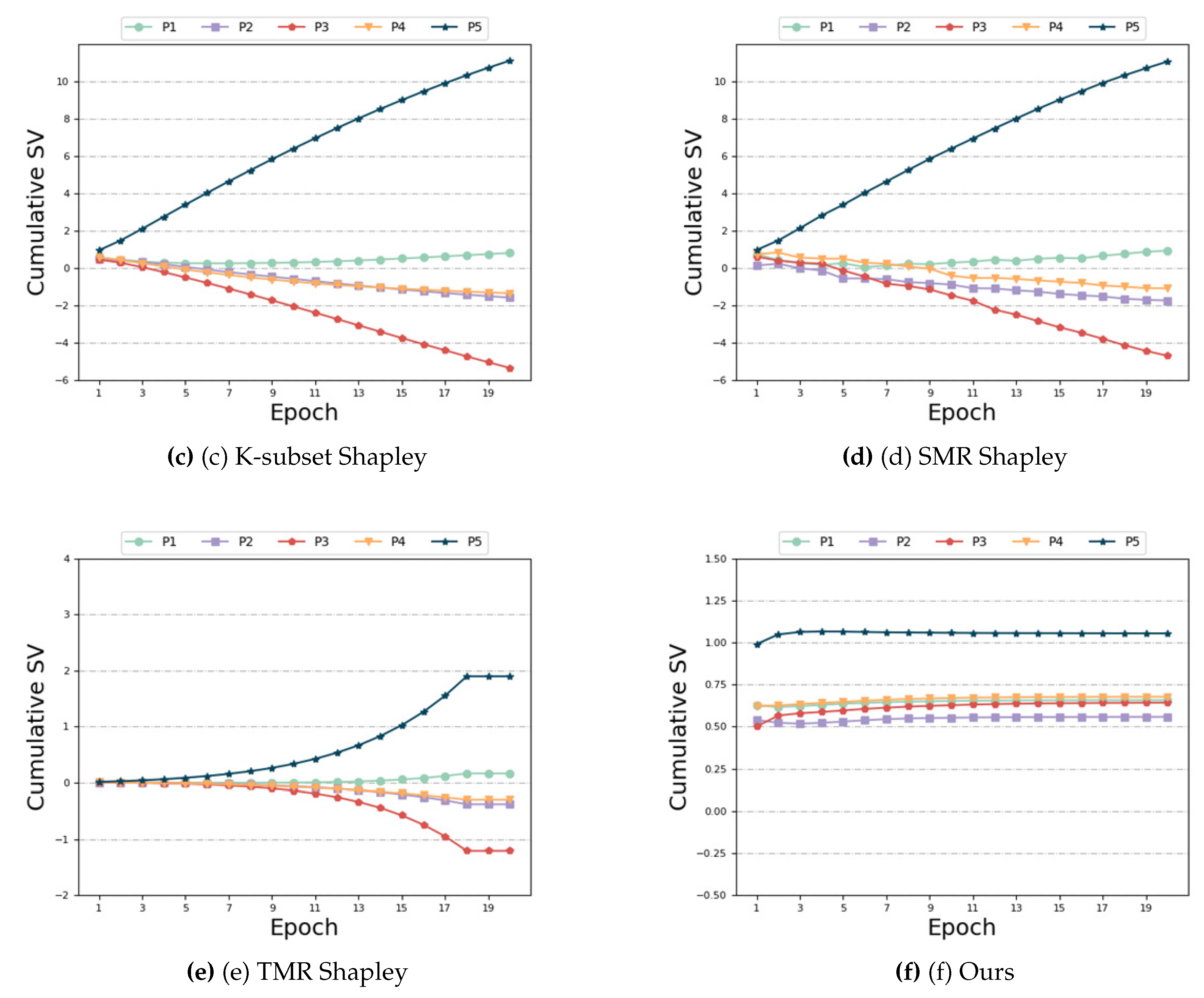
Figure 7.
Noise labels and Same size
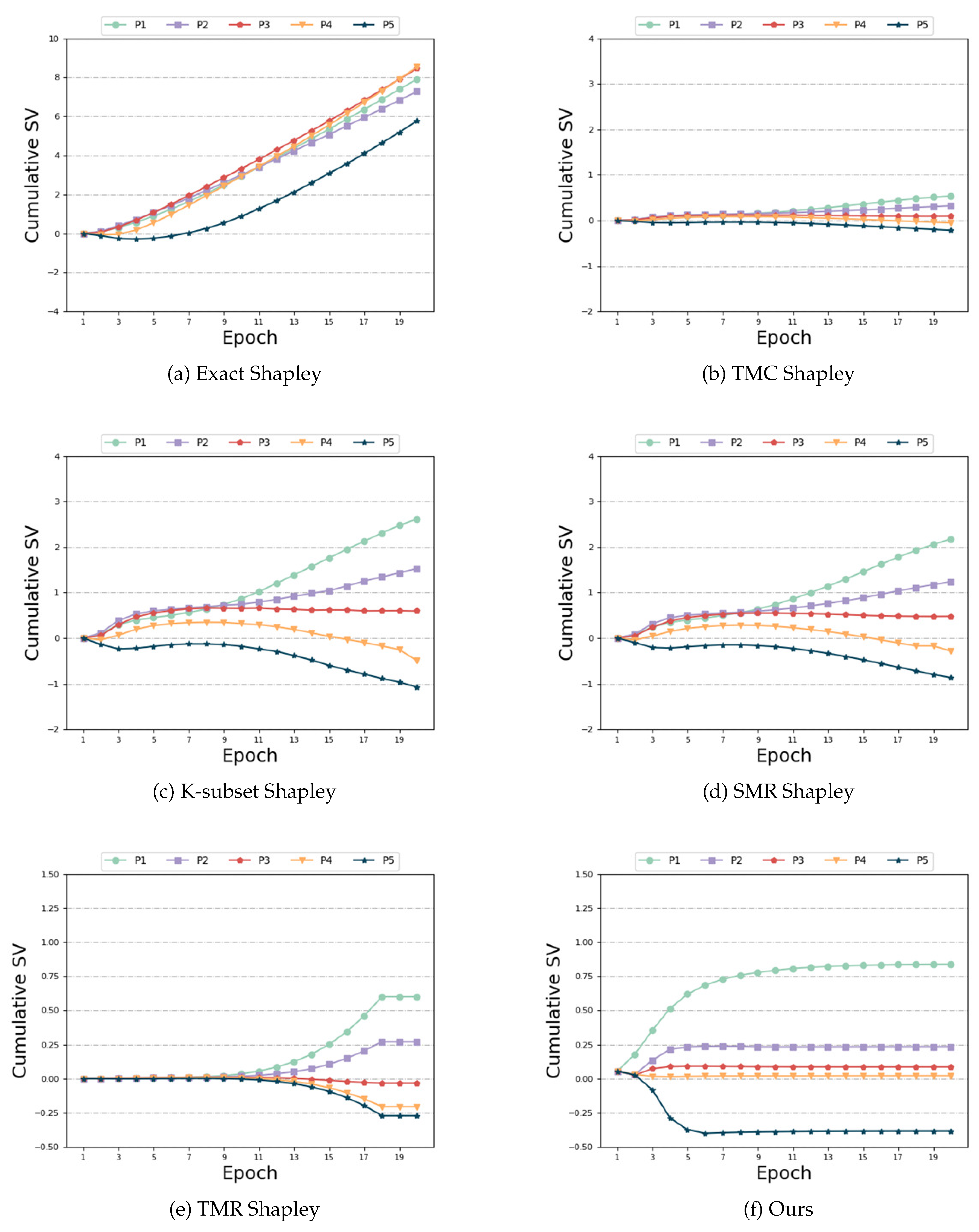

Table 1.
Time and Accuracy
| Name | Time | Accuracy |
|---|---|---|
| Exact Shapley[25] | 10840.24s | 84.93% |
| TMC Shapley[25] | 720.56s | 86.95% |
| K-subset Shapley[27] | 601.76s | 86.87% |
| SMR Shapley[6] | 636.94s | 86.70% |
| TMR Shapley[28] | 574.05s | 86.69% |
| Ours | 646.35s | 90.64% |
Table 2.
Time and Accuracy
| Name | Time | Accuracy |
|---|---|---|
| Exact Shapley[25] | 11570.86s | 85.43% |
| TMC Shapley[25] | 737.58s | 86.71% |
| K-subset Shapley[27] | 630.42s | 86.32% |
| SMR Shapley[6] | 600.94s | 86.83% |
| TMR Shapley[28] | 587.43s | 86.72% |
| Ours | 729.98s | 88.38% |
Table 3.
Time and Accuracy
| Name | Time | Accuracy |
|---|---|---|
| Exact Shapley[25] | 10865.56s | 84.42% |
| TMC Shapley[25] | 659.58s | 85.53% |
| K-subset Shapley[27] | 679.24s | 85.72% |
| SMR Shapley[6] | 695.14s | 85.83% |
| TMR Shapley[28] | 564.35s | 85.68% |
| Ours | 655.78s | 86.96% |
Disclaimer/Publisher’s Note: The statements, opinions and data contained in all publications are solely those of the individual author(s) and contributor(s) and not of MDPI and/or the editor(s). MDPI and/or the editor(s) disclaim responsibility for any injury to people or property resulting from any ideas, methods, instructions or products referred to in the content. |
© 2024 by the authors. Licensee MDPI, Basel, Switzerland. This article is an open access article distributed under the terms and conditions of the Creative Commons Attribution (CC BY) license (http://creativecommons.org/licenses/by/4.0/).
Copyright: This open access article is published under a Creative Commons CC BY 4.0 license, which permit the free download, distribution, and reuse, provided that the author and preprint are cited in any reuse.


