
Submitted:
02 June 2024
Posted:
04 June 2024
You are already at the latest version
Abstract
This paper studies the Bondi-Metzner-Sachs group in homogeneous
projective coordinates, because it is then possible to write all
transformations of such a group in a manifestly linear way.
The 2-sphere metric, Bondi-Metzner-Sachs metric, asymptotic Killing
vectors, generators of supertranslations,
as well as boosts and rotations of Minkowski spacetime, are
all re-expressed in homogeneous projective coordinates.
Last, the integral curves of vector fields which generate supertranslations
are evaluated in detail. This work prepares the ground for more advanced
applications of the differential geometry of asymptotically flat
spacetimes in projective coordinates.
Keywords:
Vector fields
; Bondi-Metzner-Sachs group
; homogeneous projective coordinates
1. Introduction
The Bondi-Metzner-Sachs [1,2,3] asymptotic symmetry group of asymptotically flat spacetime has received again much attention over the last decade by virtue of its relevance for black-hole physics [4,5,6], the group-theoretical structure of general relativity [7,8,9,10,11,12,13,14,15,16,17,18,19,20] and the infrared structure of fundamental interactions [21,22,23,24]. The appropriate geometric framework can be summarized as follows. In spacetime models for which null infinity can be defined, the cuts of null infinity are spacelike two-surfaces orthogonal to the generators of null infinity [25]. On using the familiar stereographic coordinate
the first half of Bondi-Metzner-Sachs transformations read as
where the matrix has unit determinant and belongs therefore to the group . The resulting projective version of the special linear group can be defined as the space of pairs
i.e., the group of fractional linear maps according to Eq. (2) with the associated matrix . Since
one can write that is the quotient space , where is the homeomorphism defined by
The fractional linear maps (2) can be defined for all values of upon requiring that
Moreover, under fractional linear maps, lengths along the generators of null infinity scale according to
where the conformal factor is given by [19,25]
By integration, Eq. (7) yields the second half of Bondi-Metzner-Sachs transformations:
As was pointed out in Ref. [19], the complex homogeneous coordinates associated to the Bondi-Metzner-Sachs transformation (2) have modulus , which is the equation of a unit circle, and are
In other words, upon remarking that
Eq. (2) is equivalent to the linear transformation law
The next step of the program initiated in Ref. [19] consists in realizing that, much in the same way as the affine transformations in the Euclidean plane
can be re-expressed with the help of a matrix in the form
one can further re-express Eq. (12) with the help of a matrix in the form
with the understanding that Eq. (12) is the restriction to the unit circle of the map (15), upon defining
The work in Ref. [19] has outlined the resulting geometric picture, where are viewed as homogeneous coordinates in a complex projective plane. In our paper we have instead a less abstract and more concrete task: since the Bondi-Metzner-Sachs transformation (2) becomes linear when expressed in terms of and , we are aiming to develop the Bondi-Metzner-Sachs formalism with the associated Killing vector fields by using the pair of variables instead of . For this purpose, the homogeneous projective coordinates for the 2-sphere are studied in Sect. 2, while the Bondi-Sachs metric in homogeneous coordinates is considered in Sect. 3. Asymptotic Killing fields for supertranslations are evaluated in Sect. 4, while their flow is investigated in Sect. 5. Concluding remarks and open problems are presented in Sect. 6, while technical details are provided in the Appendices.
2. Homogeneous Coordinates on the 2-Sphere
It is useful, as an instrument to develop the BMS formalism in homogeneous coordinates, to re-write the 2-sphere metric in the desired coordinates. By using the definition (10), we get
while for we obtain
By virtue of the identity
we obtain for the more convenient expression
In order to re-express the 2-sphere metric, let us evaluate
while
Eventually, we obtain the metric for the 2-sphere in homogeneous coordinates
At this stage, upon defining the real-valued function
we can write the matrix of metric components in the form
with non-vanishing determinant and inverse matrix
3. Bondi-Sachs Metric in Homogeneous Coordinates
We can now write the retarded Bondi-Sachs (hereafter BS) metric in homogeneous coordinates with the help of the previous formulae. For this purpose, let us first write the general BS metric in the form
On passing from to coordinates, we find the metric components of (3.1) expressed as follows:
The Bondi gauge implies that [26] , where is given in Eq. (2.9). With our coordinates, this relation reads as
We no longer have the simple result for the mixed component as in the stereographic coordinates, because in homogeneous coordinates we obtain
which implies that
The angular components of the metric are
where, of course, is given in Eq. (2.8). These formulae, jointly with the falloff conditions
help to rewrite
Upon assuming that , we get
while for and we find
and
where use has been made of (3.8). Eventually, we get the matrix of Bondi metric components
The gauge condition , instead of giving a solution for such as in stereographic coordinates, gives us a condition for
In order to determine the various coefficients in the falloff conditions, we require that the Bondi metric should satisfy the Einstein equations
Upon restricting to the vacuum case , in the limit as r approaches ∞ in the Einstein tensor, first looking at , and neglecting the terms of order , we get
Upon looking at and respectively, we get lengthy relations for and , compared to the stereographic coordinates case, which depend on other coefficients. However, we still manage to solve directly for and . On studying we find
and
where we recall that is given in Eq. (3.8). By virtue of Eqs. (3.12) and (3.13) we find eventually the metric in the form
Now we are ready to evaluate the BMS generators in homogeneous coordinates in order to determine the supertranslations.
4. Asymptotic Killing Fields
After finding the most general Bondi metric in homogeneous coordinates satisfying the asymptotically flat spacetime falloffs, our aim is to find the most general vector fields satisfying the Bondi gauge condition and the asymptotically flat spacetime falloffs. As is well known, the Killing vectors solve by definition the equations
Moreover, the preservation of the Bondi gauge condition yields [26]
From these relations one can calculate the four components of . At this stage, instead of repeating the detailed calculations already available, for example, in Ref. [26], we can compute the asymptotic Killing fields in homogeneous coordinates by using the familiar transformation law of vector fields. In other words, the work in Ref. [26] has defined the stereographic variable (we write rather than z used in Ref. [26], in order to avoid confusion with our in Eq. (1.1))
and has found, in Bondi coordinates , the asymptotic Killing fields where the components depend on a function f and on the Bondi coordinates. On denoting as usual by the spherical harmonics on the 2-sphere, one finds [26]
Now by virtue of the basic identities
and upon exploiting the formulae (A7)-(A10) in the Appendix, we find
Now we denote by the vector fields (4.3), (4.9), (4.10) and (4.11), respectively. Nontrivial Lie brackets among them involve only. With our notation, we can re-write Eqs. (4.9)-(4.11) in the form
where the values taken by the functions can be read off from (4.9)-(4.11). At this stage, a patient evaluation proves that such vector fields have vanishing Lie brackets:
The result is simple, but the actual proof requires several details, for which we refer the reader to Appendix B.
5. Flow of Supertranslation Vector Fields
In order to appreciate that the familiar geometric constructions are feasible also in projective coordinates, we now consider the flow of supertranslation vector fields (4.9)-(4.11). For example, by virtue of (2.7), and defining , the task of finding the flow of the supertranslation vector fields (4.9), (4.10) and (4.11) consists of solving a system of nonlinear and coupled differential equations. For this purpose, we denote by , respectively, the appropriate flow, and define
where , respectively, with components . Hence we study the following coupled systems of nonlinear differential equations:
with the initial conditions
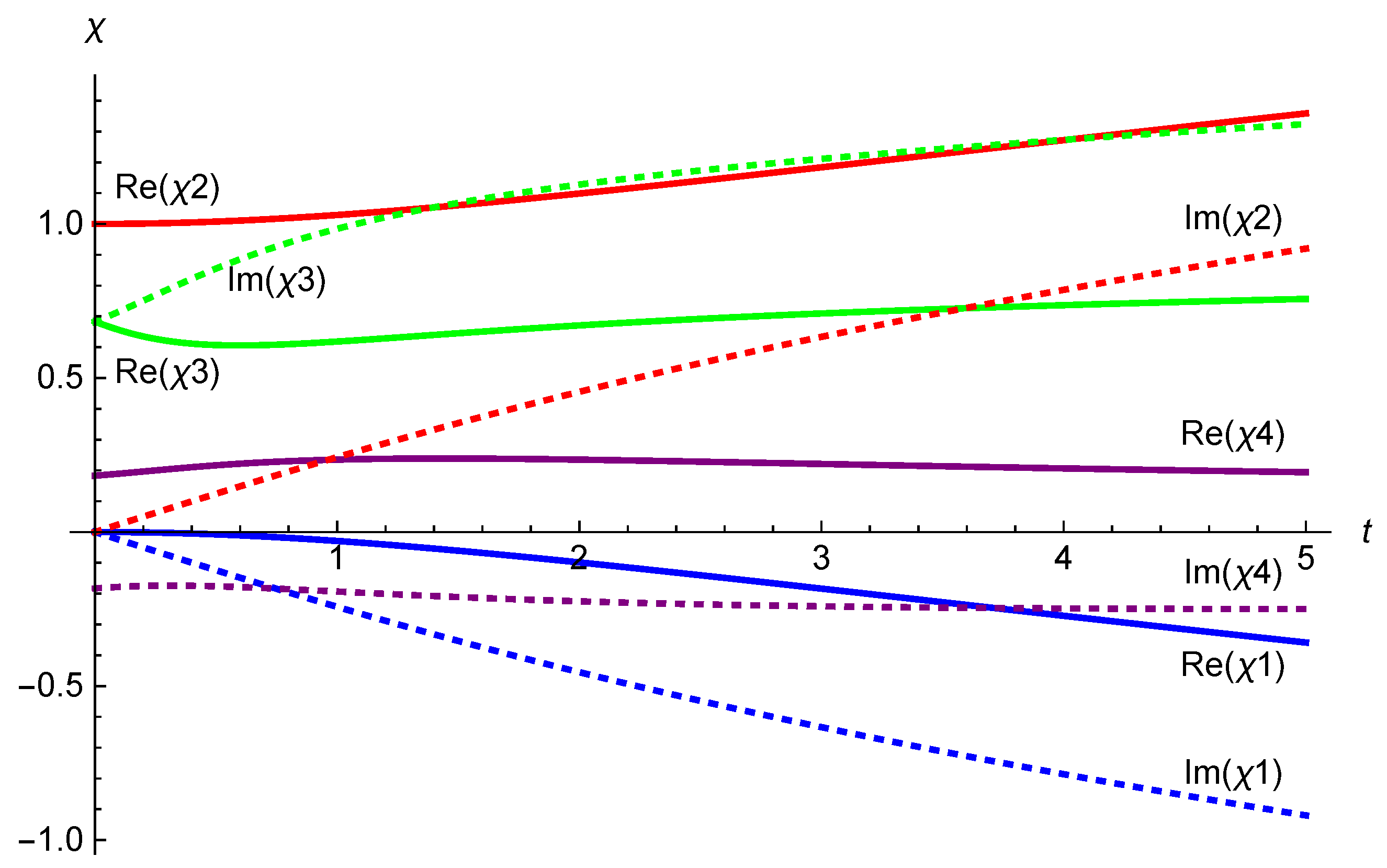
The resulting equations can only be solved numerically, to the best of our knowledge, and such solutions are displayed in Figure 1,Figure 2,Figure 3,Figure 4,Figure 5,Figure 6,Figure 7,Figure 8,Figure 9. Since the desired solutions are complex-valued, we have displayed both real and imaginary parts, with three choices of initial conditions.
6. Concluding Remarks and Open Problems
As far as we can see, the interest of our investigation lies in having shown that homogeneous projective coordinates lead to a fully computational scheme for all applications of the BMS group. This might pay off when more advanced properties will be studied. In particular, we have in mind the concept of superrotations [21,22,26] on the one hand, and the physical applications of the Segre manifold advocated in Ref. [19]. In other words, since our Eq. (1.15) contains Eq. (1.12), which in turn is just a re-expression of the BMS transformation (1.2), one might aim at embedding the study of BMS symmetries into the richer mathematical framework of complex analysis [27] and algebraic geometry. Our paper has tried to prepare the ground for such a synthesis.
Acknowledgments
The authors are grateful to Professor Patrizia Vitale for encouraging their collaboration. G. Esposito is grateful to INDAM for membership.
Appendix A. The Use of Homogeneous Coordinates
By virtue of Eqs. (1.10) and (2.7), we find
and hence the variable in Eq. (4.2) can be re-expressed in the form
while
Moreover, we need the identities
which, jointly with the definitions (1.10), lead to
At this stage, we can evaluate the partial derivatives occurring in Eqs. (4.7) and (4.8) by patient application of Eqs. (A2), (A3) and (A6), i.e.,
and we find eventually the asymptotic Killing fields in the form (4.9)-(4.11). Our homogeneous projective coordinates and have also been considered in Ref. [28], but in that case, upon writing
one finds that the coordinates for the embedding of the 2-sphere in three-dimensional Euclidean space are given by
The global spacetime translations of Minkowski spacetime can be first re-expressed in coordinates, and read eventually, in terms of the asymptotic Killing fields (4.9)-(4.11),
Explicitly, we find
Appendix B. Lie Brackets of Asymptotic Killing Fields
Given the vector fields (4.12) and (4.13), the evaluation of their Lie bracket shows that
where, upon defining the functions
we find that
In the course of performing the calculation, the definition (2.7) leads to the useful identity
An analogous procedure shows that
with the help of two additional sets of 14 nonvanishing functions, one set for each Lie bracket in (B20). For example, in the Lie bracket among and , the coefficient of is a function
References
- H. Bondi, M.G.J. Van der Burg, A.W.K. Metzner, Gravitational waves in general relativity. VII. Waves from axi-symmetric isolated systems, Proc. Roy. Soc. London A 269, 21 (1962).
- R.K. Sachs, Gravitational waves in general relativity. VIII. Waves in asymptotically flat space-time, Proc. Roy. Soc. London A 270, 103 (1962).
- R.K. Sachs, Asymptotic symmetries in gravitational theory, Phys. Rev. 128, 2851 (1962).
- S.W. Hawking, M.A. Perry, A. Strominger, Soft hair on black holes, Phys. Rev. Lett. 116, 231301 (2016). [CrossRef]
- S.W. Hawking, M.A. Perry, A. Strominger, Superrotation charge and supertranslation hair on black holes, JHEP 2017 5, 161 (2017). [CrossRef]
- S. Haco, S.W. Hawking, M.A. Perry, A. Strominger, Black hole entropy and soft hair, JHEP 2018 12, 98 (2018).
- P.J. McCarthy, Representations of the Bondi-Metzner-Sachs group I. Determination of the representations, Proc. Roy. Soc. London A 330, 517 (1972).
- P.J. McCarthy, Structure of the Bondi-Metzner-Sachs group, J. Math. Phys. 13, 1837 (1972).
- P.J. McCarthy, Representations of the Bondi-Metzner-Sachs group II. Properties and classification of representations, Proc. Roy. Soc. London A 333, 317 (1973).
- P.J. McCarthy, M. Crampin, Representations of the Bondi-Metzner-Sachs group III. Poincaré spin multiplicities and irreducibility, Proc. Roy. Soc. London A 335, 321 (1973). [CrossRef]
- P.J. McCarthy, M. Crampin, Representations of the Bondi-Metzner-Sachs group IV. Cantoni representations are induced, Proc. Roy. Soc. London A 351, 55 (1976).
- G. Barnich, C. Troessaert, Finite BMS transformations, JHEP 2016 3, 167 (2016).
- F. Alessio, G. Esposito, On the structure and applications of the Bondi-Metzner-Sachs group, Int. J. Geom. Methods Mod. Phys. 15, 1830002 (2018). [CrossRef]
- M. Henneaux, C. Troessaert, BMS group at spatial infinity. The Hamiltonian (ADM) approach, JHEP 2018 3, 147 (2018).
- G. Barnich, K. Nguyen, R. Ruzziconi, Geometric action of extended Bondi-Metzner-Sachs group in four dimensions, JHEP 2022 12, 154 (2022).
- C. Chowdhury, A. Anupam, A. Kundu, Generalized BMS algebra in higher even dimensions, Phys. Rev. D 106, 126025 (2022).
- O. Fuentealba, M. Henneaux, J. Matulich, C. Troessaert, Bondi-Metzner-Sachs group in five spacetime dimensions, Phys. Rev. Lett. 128, 051103 (2022).
- D. Prinz, A. Schmeding, Lie theory for asymptotic symmetries in general relativity: The BMS group, Class. Quantum Grav. 39, 065004 (2022).
- Z. Mirzaiyan, G. Esposito, On the nature of Bondi-Metzner-Sachs transformations, Symmetry 15, 947 (2023). [CrossRef]
- D.A. Weiss, A microscopic analogue of the BMS group, JHEP 2023 4, 136 (2023).
- A. Strominger, Lectures on the Infrared Structure of Gravity and Gauge Theory (Princeton University Press, Princeton, 2018).
- S. Pasterski, Implications of superrotations, Phys. Rep. 829, 1 (2019).
- E. Himwich, Z. Mirzaiyan, S. Pasterski, A note on the subleading soft graviton, JHEP 2021 4, 172 (2021).
- G. Compère, S.E. G. Compère, S.E. Gralla, An asymptotic framework for gravitational scattering, Class. Quantum Grav. 40, 205018 (2023).
- J.M. Stewart, Advanced General Relativity (Cambridge University Press, Cambridge, 1990).
- X. Kervyn, BMS Symmetries of Gravitational Scattering, https://arxiv.org/abs/2308.12979, gr-qc (2023).
- G. Della Sala, A. Saracco, A. Simioniuc, G. Tomassini, Lectures on Complex Analysis and Analytic Geometry (Scuola Normale Superiore, Pisa, 2006).
- R. Penrose, W. Rindler, Spinors and Space-Time. 1: Two-Spinor Calculus and Relativistic fields (Cambridge University Press, Cambridge, 1984).
Figure 1.
Numerical evaluation of the integral curve for the supertranslation vector field (4.9). The initial conditions (5.14) are taken to be .
Figure 1.
Numerical evaluation of the integral curve for the supertranslation vector field (4.9). The initial conditions (5.14) are taken to be .
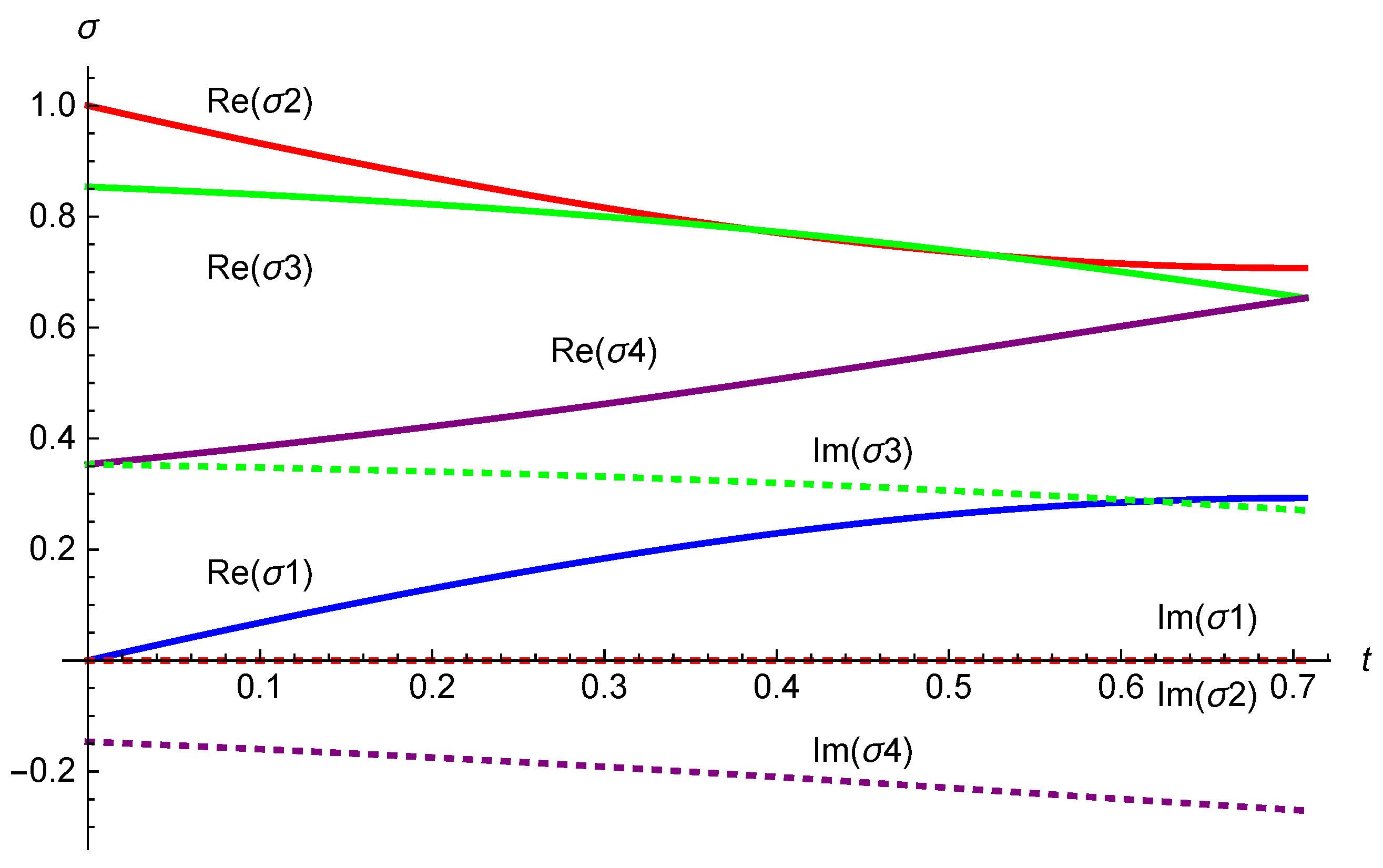
Figure 2.
Numerical evaluation of the integral curve for the supertranslation vector field (4.10). The initial conditions (5.14) are taken to be .
Figure 2.
Numerical evaluation of the integral curve for the supertranslation vector field (4.10). The initial conditions (5.14) are taken to be .
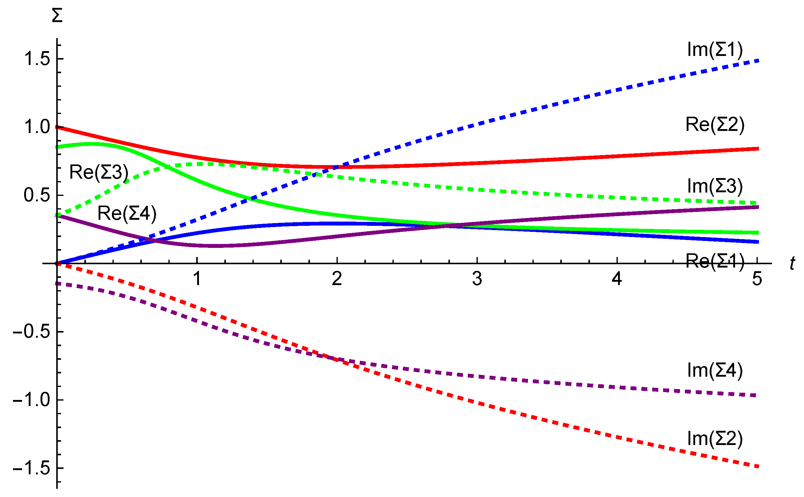
Figure 3.
Numerical evaluation of the integral curve for the supertranslation vector field (4.11). The initial conditions (5.14) are taken to be .
Figure 3.
Numerical evaluation of the integral curve for the supertranslation vector field (4.11). The initial conditions (5.14) are taken to be .
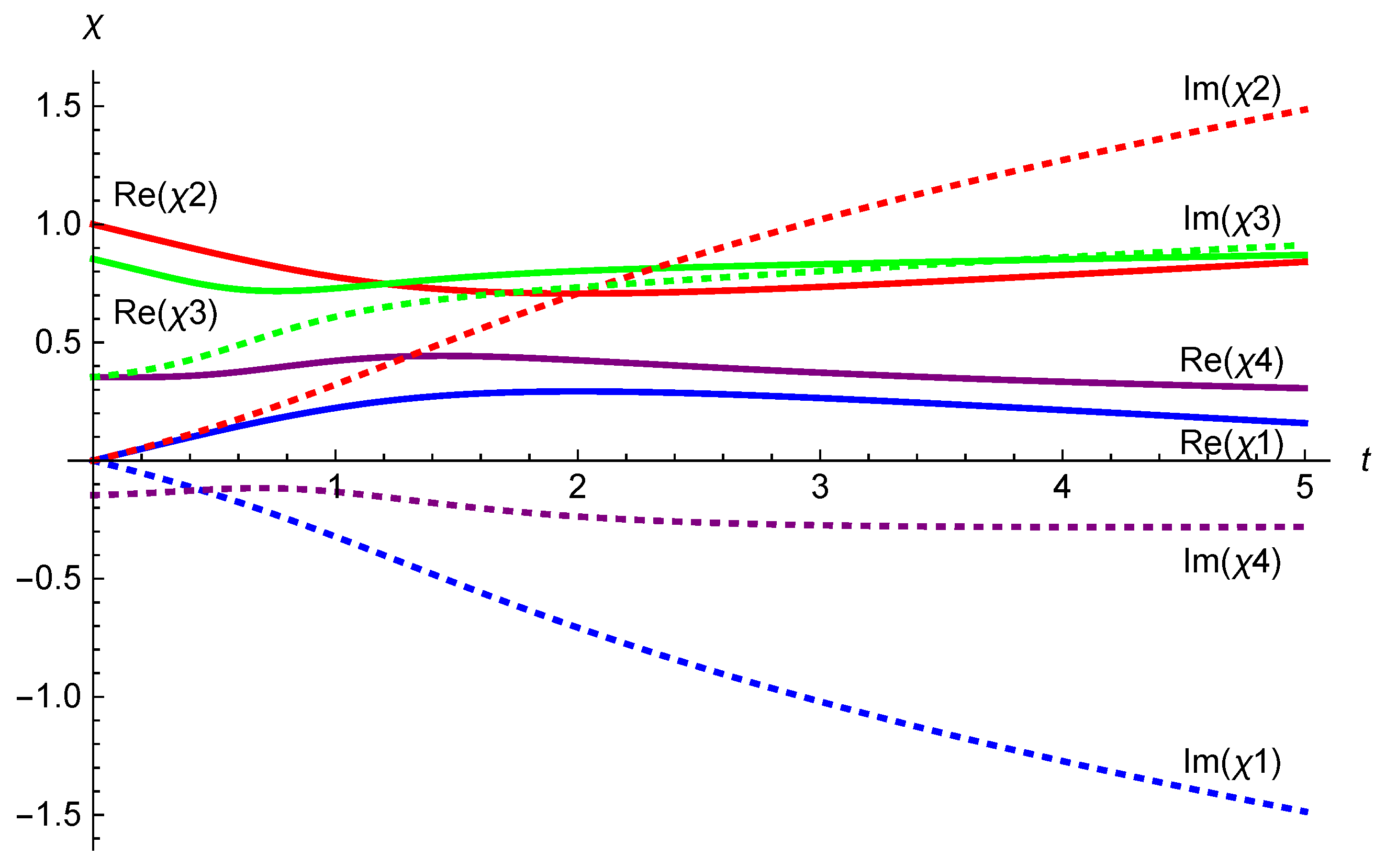
Figure 4.
Numerical evaluation of the integral curve for the supertranslation vector field (4.9). The initial conditions (5.14) are taken to be .
Figure 4.
Numerical evaluation of the integral curve for the supertranslation vector field (4.9). The initial conditions (5.14) are taken to be .
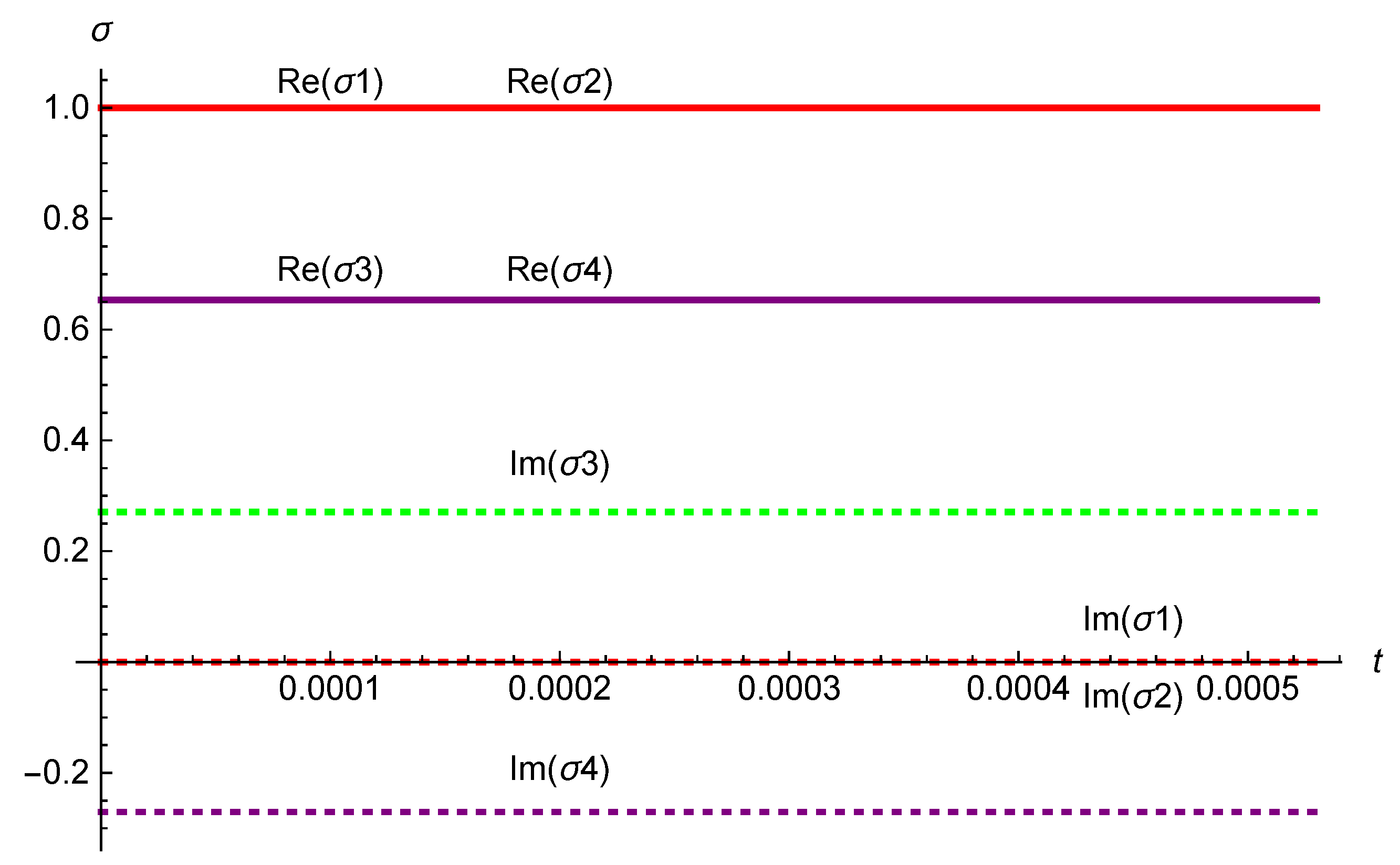
Figure 5.
Numerical evaluation of the integral curve for the supertranslation vector field (4.10). The initial conditions (5.14) are taken to be .
Figure 5.
Numerical evaluation of the integral curve for the supertranslation vector field (4.10). The initial conditions (5.14) are taken to be .
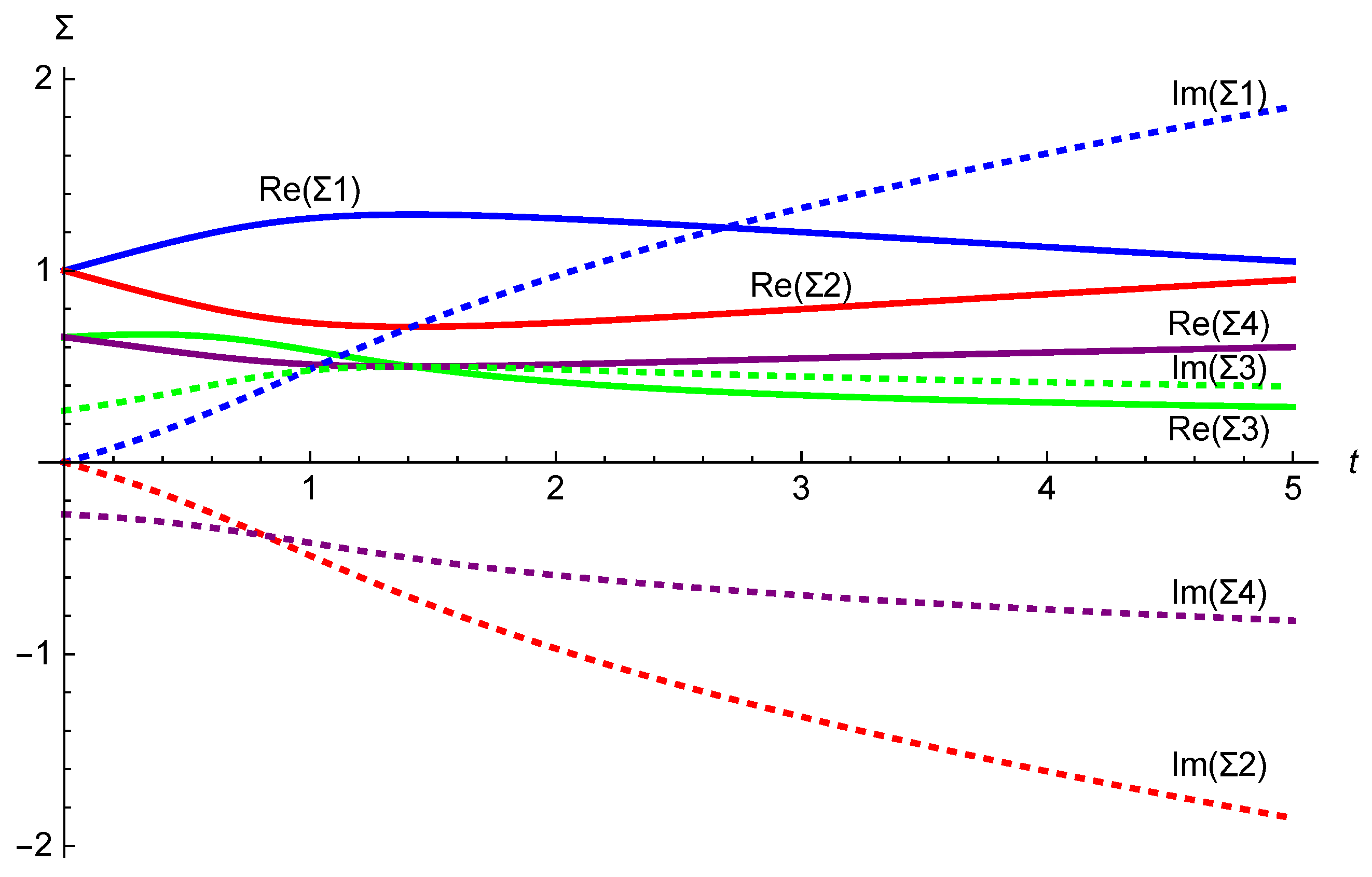
Figure 6.
Numerical evaluation of the integral curve for the supertranslation vector field (4.11). The initial conditions (5.14) are taken to be .
Figure 6.
Numerical evaluation of the integral curve for the supertranslation vector field (4.11). The initial conditions (5.14) are taken to be .
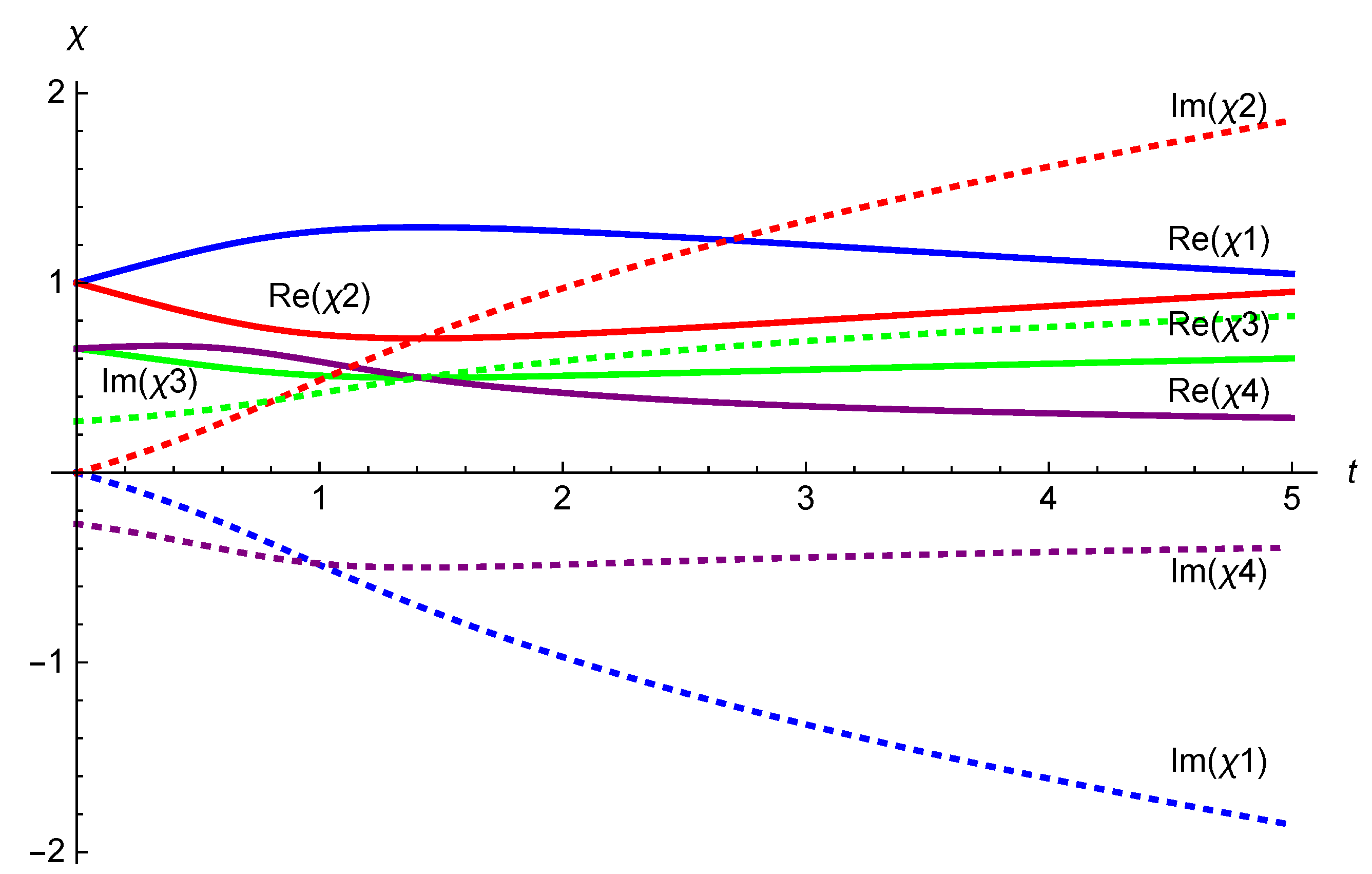
Figure 7.
Numerical evaluation of the integral curve for the supertranslation vector field (4.9). The initial conditions (5.14) are taken to be . In this particular case, the real parts meet at a single point.
Figure 7.
Numerical evaluation of the integral curve for the supertranslation vector field (4.9). The initial conditions (5.14) are taken to be . In this particular case, the real parts meet at a single point.
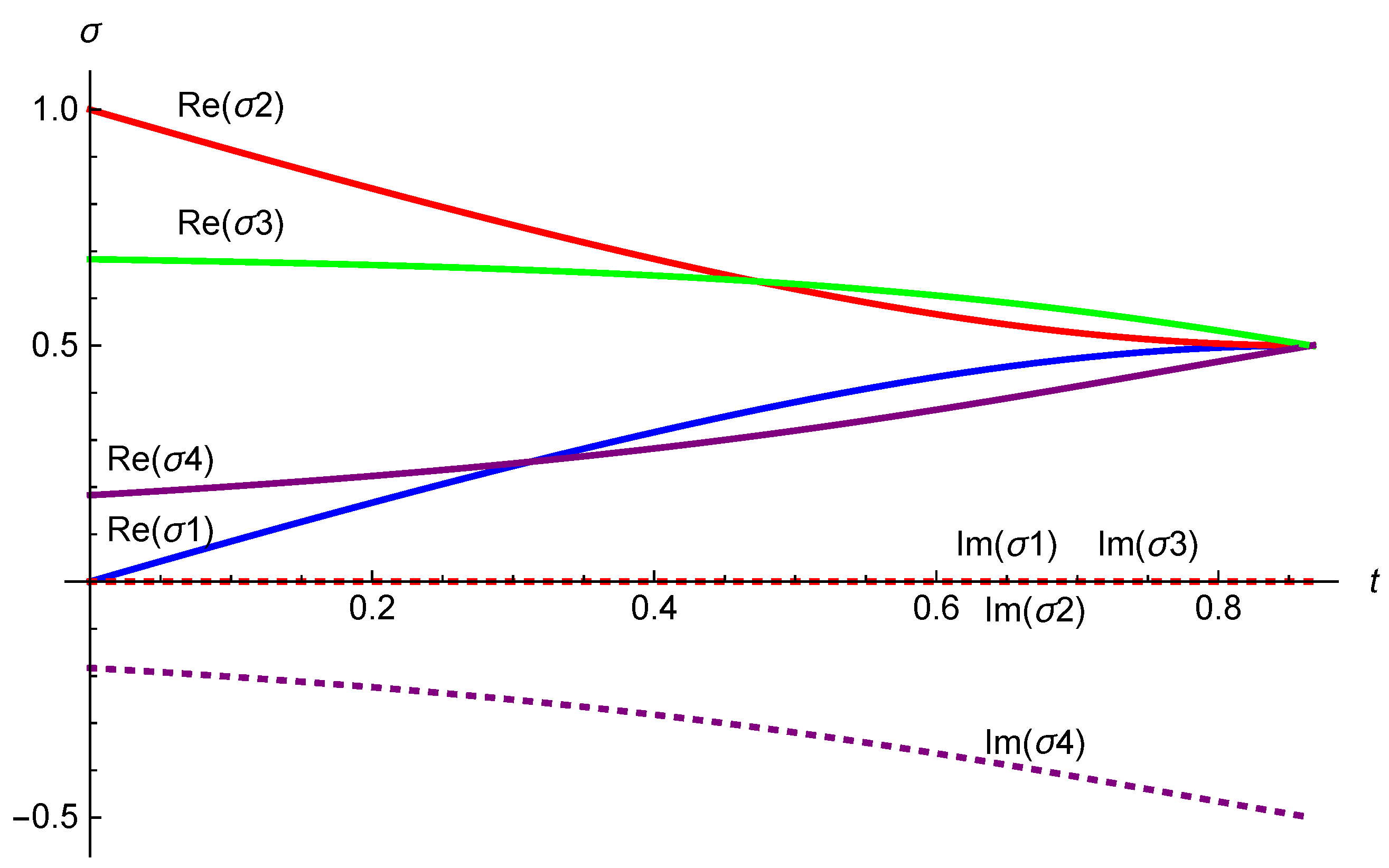
Figure 8.
Numerical evaluation of the integral curve for the supertranslation vector field (4.10). The initial conditions (5.14) are taken to be .
Figure 8.
Numerical evaluation of the integral curve for the supertranslation vector field (4.10). The initial conditions (5.14) are taken to be .
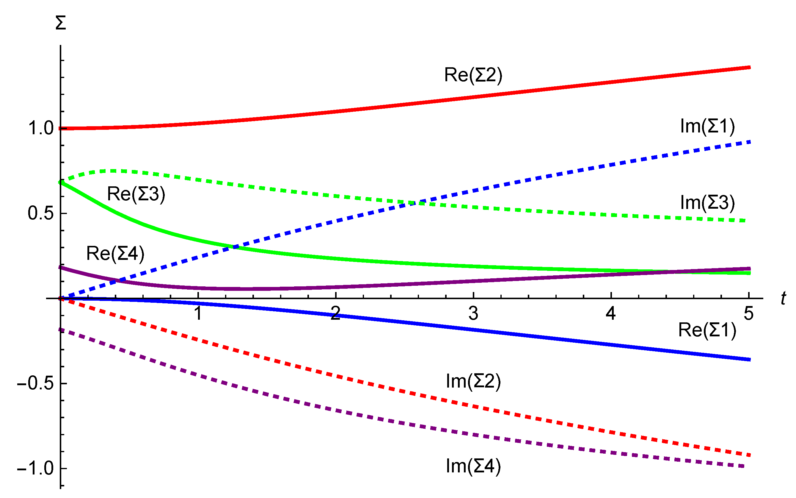
Figure 9.
Numerical evaluation of the integral curve for the supertranslation vector field (4.11). The initial conditions (5.14) are taken to be .
Figure 9.
Numerical evaluation of the integral curve for the supertranslation vector field (4.11). The initial conditions (5.14) are taken to be .
Disclaimer/Publisher’s Note: The statements, opinions and data contained in all publications are solely those of the individual author(s) and contributor(s) and not of MDPI and/or the editor(s). MDPI and/or the editor(s) disclaim responsibility for any injury to people or property resulting from any ideas, methods, instructions or products referred to in the content. |
© 2024 by the authors. Licensee MDPI, Basel, Switzerland. This article is an open access article distributed under the terms and conditions of the Creative Commons Attribution (CC BY) license (http://creativecommons.org/licenses/by/4.0/).
Copyright: This open access article is published under a Creative Commons CC BY 4.0 license, which permit the free download, distribution, and reuse, provided that the author and preprint are cited in any reuse.