Integrating Mathematical Optimization to Enhance Sustainability in a Crop and Dairy Production Agent-Based Model for Luxembourg

1. Introduction

The agriculture sector accounts for approximately 54% of total methane emissions in the EU and nearly 79% of total N₂O emissions [1], and at the global (world) level, it is responsible for 16.5% of total greenhouse gas (GHG) emissions [2], besides affecting several other environmental impact categories besides climate change. Therefore, it is a non-negligible sector to apply sustainability-oriented policies.

Nevertheless, modeling efforts are required to capture new features arising from the interactions among the many actors engaged in agricultural production systems due to their complexity. In this respect, agent-based models (ABM) allow the consideration of different actors and the exploration of their reciprocal interactions at the micro- (farmer's level) or macro-level (regional or national) [3]. The agents are autonomous entities that may be physical or virtual [4]. They follow a broad set of rules within an environment where learning and adaptation can also generate changes in other agents or the environment [5]. However, in the literature the applications of ABMs go beyond agrifood systems and cover most coupled human-natural systems (CHANS) [6], including socio-economic, techno-social and environmental systems [7,8,9,10,11,12,13,14,15].

Because of their fitness to deal with complex systems, ABM have been proposed in combination with environmental life cycle assessment (simply called LCA hereafter) to model the evolution of agricultural systems and at the same time assess their sustainability holistically, i.e. across all their phases [16]. This is motivated by the fact that LCA is a standardized methodology able to quantify impacts of a product or a service in its entire life cycle, in the so-called areas of protection (AoP) resources, ecosystems and human health [17].

In this work, we enhance the model presented in [18] by using mathematical programming (MP) to optimize the farm business, considering not only the economic dimension but also the environmental one, tackled from a LCA-based perspective, i.e. by encompassing the entire production and supply chain and not just the farm-based phase. The advantage of a lifecycle-based approach is that it allows to identify possible hotspots, preventing the shifting of environmental burdens (i.e. the generation of environmental impacts and the consumption of natural resources) from the farm operation phase to other phases outside of the control of the farm manager [19].

2. Materials and Methods

The model simulates the activities of 1872 farms in Luxembourg, including livestock (dairy and meat production) and crop farming activities and integrating a mathematical optimization of each farm at every time step based on economic and environmental objectives and constraints.

The environmental impact assessment of farmers’ decisions is carried out using the Environmental Footprint (EF) 3.0 method [41].

In our model, the objective function that each agent uses to optimize its operations includes EF impact scores on one or multiple impact categories, which are normalized and weighted, using the normalization and weighting factors listed in Table 1 of the S4 file, to calculate a single score value.

The time step used in our simulations is one month, and the simulation covers the span of ten years. This time step was chosen because crop rotation changes occur at different moments of the year, and 1-month time step allows to follow more precisely harvesting and planting decisions for each crop. Furthermore, decisions that impact the structure of the herd (for example, culling decisions) are made by the farmer monthly rather than on an annual basis. Finally, crop, milk, and meat prices all have seasonal patterns that may impact farmer decisions. Crop fertilizer requirements can be met in a variety of ways. The first alternative is to use either solid or liquid farm-produced animal manure. The second option is to purchase inorganic fertilizers at a set price during the experiment. Dairy farms, which account for most farms in Luxembourg, use animal manure first and then purchase inorganic fertilizer if the crop requires further fertilization. Farmers who are members of a biogas cooperative may use the digestate from the biogas facility as a third alternative. However, due to a lack of precise farm-specific data, the model provided in this research does not incorporate biogas producing operations. The costs included in the model are divided into two categories: fixed and variable. Fixed costs are those primarily determined by the size of the farm, such as material costs, fixed capital consumption, cost of labor, and energy costs, which are not taken into consideration in the optimization owing to a lack of accurate data. Variable expenses, on the other hand, are those that vary according on the number of animals and the cultivated area, such as fertilizers, animal feed, plant seeds, and veterinary charges.

The animals in our model are represented individually, which means that their phenotypical traits (body weight, gender, age, etc.) are allocated to each cattle head separately. Body weight estimate is needed to calculate an animal's energy requirements. As a result, we proceeded in two stages. First, we used the body weight mid infrared based calculation provided by for dairy cows developed by [42] on the Walloon milk spectral database managed by the Walloon Breeding Association. This database contained 713,428 records (45,488 cows and 222 herds) collected from 2006 to 2020. The predicted body weight was then modeled using (1) where the independent variables (weeks of breastfeeding and parity) were classified into five classes (first to fifth+ parity, i.e., we set to 5 every parity larger than 5). Based on parity and week of breastfeeding, this equation reflects the theoretical averaged calculation of expected BW. Table 1 shows the coefficients of the equation utilized to perform the BW simulation.

$$BW \left(kg\right)={\mathrm{y}}_{\mathrm{i}\mathrm{n}\mathrm{t}\mathrm{e}\mathrm{r}\mathrm{c}\mathrm{e}\mathrm{p}\mathrm{t}}+w_1{n}_{parity}+w_{2}WOL+w_3{WOL}^2+w_4{WOL}^3+w_5{WOL}^4+w_6{WOL}^5$$

(1)

where $n_{parity}$ is the number of parities (i.e. the number of gestations a cow has completed) of the animal and WOL is the week of lactation.

Table 1. The coefficients for (1) that is used to calculate the body weight of dairy animals.

	Yintercept	w1	w2	w3	w4	w5	w6
Mean	539.344995	37.1976496	-8.204927	0.98199403	-0.0470851	0.00102944	-0.00000831
St. Dev.	0.32182335	0.0275649	0.130811	0.01723356	0.00095285	0.00002321	0.000000205

Table 1. The coefficients for (1) that is used to calculate the body weight of dairy animals.

	Yintercept	w1	w2	w3	w4	w5	w6
Mean	539.344995	37.1976496	-8.204927	0.98199403	-0.0470851	0.00102944	-0.00000831
St. Dev.	0.32182335	0.0275649	0.130811	0.01723356	0.00095285	0.00002321	0.000000205

2.1. Multi-Objective Optimization Problem (MOOP) Formulation

In the S3 file, the definition of mathematical optimization, a generic explanation of linear programming, weighted sum method and details of how NSGA-III works can be found. In this section, we will introduce the problem formulation, i.e., the objectives and constraints of the MOOP.

The NSGA III method was used to implement the MOO in this work. We employed the multi objective evolutionary algorithm (MOEA) framework [43], an open-source Java library that supports multiple evolutionary algorithms, including NSGA III. This choice was considered suitable for our case, because our agent-based simulator is written in Java [44]. The probabilities of crossover [45] and mutation [46] were set to 0.9 and 0.1, respectively. The algorithm's convergence is dependent on the population size (N). This latter can affect the efficiency of evolution, preventing iteration from stopping at local optima. A population of 100 individuals can be attained in a reasonable period of processing time, and increasing the size has little effect on the answers.

The ideal values for various decisions, such as the number of animals to keep in the farm at each iteration, or cropland allocation to different crops, are established by solving the objective functions. The optimization module is run in the post-market phase, i.e. when the revenues for the sales of the farm produce have been already calculated. Table 2 lists the variables used in the optimization problem.

Table 2. Variables used in the optimization problem.

Indices and sets		Units
t	index for the planning time step	—
c	index for crop products	—
A	index for animals	—
I	index for environmental impact categories	—
C	set of crops	—
NC	size of current crop plantation	—
NLnewborn	number of newborns	—
NLcull	number of livestock to be culled	—
Decision variables
UAAc,t	Utilized agricultural area (UAA) with crop plantation c for a given time t.	ha
NL	number of livestock	—
Parameters
T	simulation time horizon.	years
hc	harvesting month of crop c.	—
sc	seeding month of crop c.	—
Af	total acreage available in farm f.	ha
wi	weight of the EF impact category i	—
ni	normalization factor of the EF impact category i	—
impc,i	environmental impact of crop c in impact category i	—
impmilk,i	environmental impact of milk in impact category i	—
impmeat,i	environmental impact of meat in impact category i	—
Continuous variables
fc,t	profit from crop production at time t.	€
fa,t	profit from animal production at time t.	€
fs,t	revenue from subsidies at time t.	€
fp,t	total profit of a farm at time t.	€
fi,t	impact of farming activities for impact category i at time t.	—
fEF,t	EF single score impact of farming activities at time t.	—
pc,t	price of crop c sold at time t.	€/ha
vcc,t	variable cost of production of crop c sold at time t.	€/ha
Ac,t	area of crop c at time t.	ha
Apasture,t	area occupied by pastureland at time t.	ha
pmilk,t	price of milk sold at time t.	€/kg
ymilk,t	total yield of milk at time t.	kg
pmeat,t	price of meat sold at time t.	€/kg
ymeat,t	total yield of meat at time t.	kg
vcfeed,t	variable cost of feeding at time t.	€
vcvet,t	variable cost of veterinary at time t.	€
Pmilk,t	total milk production in the farm at time t.	kg
Pmilk,a,t	total milk production of animal a at time t.	kg
Pmeat,t	total meat production in the farm at time t.	kg
Pmeat,a,t	total meat production from animal a at time t.	kg
m	the current month of the simulation	—
mp	the number of months to be considered for rolling sum profit	—
fp,roll	mp-month rolling sum of farm profit.	€
NEroll	12-month rolling sum of nitrogen excretion.	kg
NEt	nitrogen excretion at the current time t.	kg
subt	total subsidies received by the farmer at time t.	€
Mt	transition matrix for fields at time t.	—

Table 2. Variables used in the optimization problem.

Indices and sets		Units
t	index for the planning time step	—
c	index for crop products	—
A	index for animals	—
I	index for environmental impact categories	—
C	set of crops	—
NC	size of current crop plantation	—
NLnewborn	number of newborns	—
NLcull	number of livestock to be culled	—
Decision variables
UAAc,t	Utilized agricultural area (UAA) with crop plantation c for a given time t.	ha
NL	number of livestock	—
Parameters
T	simulation time horizon.	years
hc	harvesting month of crop c.	—
sc	seeding month of crop c.	—
Af	total acreage available in farm f.	ha
wi	weight of the EF impact category i	—
ni	normalization factor of the EF impact category i	—
impc,i	environmental impact of crop c in impact category i	—
impmilk,i	environmental impact of milk in impact category i	—
impmeat,i	environmental impact of meat in impact category i	—
Continuous variables
fc,t	profit from crop production at time t.	€
fa,t	profit from animal production at time t.	€
fs,t	revenue from subsidies at time t.	€
fp,t	total profit of a farm at time t.	€
fi,t	impact of farming activities for impact category i at time t.	—
fEF,t	EF single score impact of farming activities at time t.	—
pc,t	price of crop c sold at time t.	€/ha
vcc,t	variable cost of production of crop c sold at time t.	€/ha
Ac,t	area of crop c at time t.	ha
Apasture,t	area occupied by pastureland at time t.	ha
pmilk,t	price of milk sold at time t.	€/kg
ymilk,t	total yield of milk at time t.	kg
pmeat,t	price of meat sold at time t.	€/kg
ymeat,t	total yield of meat at time t.	kg
vcfeed,t	variable cost of feeding at time t.	€
vcvet,t	variable cost of veterinary at time t.	€
Pmilk,t	total milk production in the farm at time t.	kg
Pmilk,a,t	total milk production of animal a at time t.	kg
Pmeat,t	total meat production in the farm at time t.	kg
Pmeat,a,t	total meat production from animal a at time t.	kg
m	the current month of the simulation	—
mp	the number of months to be considered for rolling sum profit	—
fp,roll	mp-month rolling sum of farm profit.	€
NEroll	12-month rolling sum of nitrogen excretion.	kg
NEt	nitrogen excretion at the current time t.	kg
subt	total subsidies received by the farmer at time t.	€
Mt	transition matrix for fields at time t.	—

The goal of the model is to reduce the environmental impact while maximizing profit from milk and dairy products and crops at the farm level. Crop production profit is computed as the difference between revenue and variable costs of cropping operations:

$$f_{c,t}=\sum _{c,t}{p}_{c,t}{A}_{c,t}-\sum _{c,t}v{c}_{c,t}{A}_{c,t}$$

(2)

To calculate the total milk and meat production, individual productions of animals are first calculated and then aggregated over the farm.

$$P_{milk,t}=\sum _a{P}_{milk,a,t}$$

(3)

$$P_{meat,t}=\sum _a{P}_{meat,a,t}$$

(4)

The profit for animal production is calculated similarly to crops by subtracting the variable costs of veterinary and feeding spending from the revenue:

$$f_{a,t}=\sum _t{p}_{milk,t}{P}_{milk,t}+\sum _t{p}_{meat,t}{P}_{meat,t}-\sum _{a,t}v{c}_{vet, a,t}-\sum _{a,t}v{c}_{feed, a,t}$$

(5)

The subsidy schemes explained in [18] are still in place. Therefore, they are part of a farm revenue stream. However, the amount of subsidy for compensatory allowance has been recently changed. Farmers get 165 €/ha up to 90 ha and 90 €/ha above 90 ha.

$$f_{s,t}=\sum _{t}su{b}_t$$

(6)

Then we define the first objective function as:

$$f_{p,t}=f_{a,t}+f_{c,t}+f_{s,t}$$

(7)

The environmental impacts are calculated using the impact scores of crops and animal production activities. As mentioned above, the EF 3.0 LCIA method was used to formulate the optimization problem. The objective function may include more than one impact category. Its expression for one category can be written as follows:

$$f_{i,t}=\sum _{t,i}{y}_{milk,t}im{p}_{milk,i}+\sum _{t,i}{y}_{meat,t}im{p}_{meat,i}+\sum _{t,i}{A}_{c,t}im{p}_{c,i}$$

(8)

The EF single score impact of a farm ($f_{EF})$ were calculated using the weights in Table 1 of the S4 file:

$$f_{EF,t}=\sum _{t,i}\frac{f_{i,t}}{n_i}{w}_i$$

(9)

Each farm is assigned a certain number of fields, or unitary agricultural areas (UAAs1). During the simulations, the extension and boundaries of a farm or the geometry of fields are not modified (because fields cannot be sold or split). As a result, the size of a farm is always equal to or larger than the cultivated area:

$$\sum _c{A}_{c,t}\le A_f\forall t$$

(10)

By regulation, the pastureland total area cannot change and pastures cannot be turned into cropland:

$$A_{pasture,t}=A_{pasture, t-1} \forall t$$

(11)

Crop harvesting and sowing are subjected to several constraints. Transitioning from one agricultural plantation to another is only possible during the harvesting and sowing seasons of the related crops. Furthermore, a farm's crop rotation scheme must be respected. Farmers can pick crops with lesser environmental impacts if the value of their green consciousness (GC) parameter (see Table 6) is greater than the threshold that was set (0.5 in all tests in this study). If not, they select the most lucrative option while keeping the plantation calendar and crop rotation scheme limits in mind.

If M is the transition matrix (the matrix containing the probability of changing crops), then the transition from crop x to crop y can take place as:

$${UAA}_{C_y,t+1}=M_t^{x,y}{UAA}_{C_x,t}$$

(12)

where each element of $M_t$ (i.e., $M_t^{x,y}$) is determined according to crop rotation and the GC value of the farmer. (12) is also subject to the constraints:

$$h_x-1 \le \mathrm{m}\le h_x+1$$

(13)

$$s_y-1 \le \mathrm{m}\le s_y+1$$

(14)

Therefore, the harvesting and sowing seasons for current and following crop plantations are considered respectively in transitioning.

Dairy producers must choose which animals to cull and how many. If the culling decisions in our model are not controlled, two major issues may arise. First, while animals must always be culled owing to age constraints, farmers may desire to cull more animals to receive more subsidies or reduce adverse environmental effects. The other issue is the exact opposite of excessive culling. Farmers may wish to raise herd size to boost milk output and therefore optimize profit. As a result, the number of culled animals is limited by the number of births and farm class (Table 3).

Table 3. The constraints on culling decisions.

Farm class	Culling condition	Culling decision
	${NL}_{newborn}-1\le {NL}_{cull}\le {\mathrm{N}L}_{newborn}+1$ (15)	${NL}_{cull}$
A,B,C,D	${NL}_{cull}\le {NL}_{newborn}-1$ (16)	${NL}_{newborn}-1$
	${NL}_{cull}\ge {NL}_{newborn}+1$ (17)	${NL}_{newborn}+1$
	${NL}_{newborn}-2\le {NL}_{cull}\le {NL}_{newborn}+2$ (18)	${NL}_{cull}$
E,F,G,H	${NL}_{cull}\le {NL}_{newborn}-2$ (19)	${NL}_{newborn}-2$
	${NL}_{cull}\ge {NL}_{newborn}+2$ (20)	${NL}_{newborn}+2$

Table 3. The constraints on culling decisions.

Farm class	Culling condition	Culling decision
	${NL}_{newborn}-1\le {NL}_{cull}\le {\mathrm{N}L}_{newborn}+1$ (15)	${NL}_{cull}$
A,B,C,D	${NL}_{cull}\le {NL}_{newborn}-1$ (16)	${NL}_{newborn}-1$
	${NL}_{cull}\ge {NL}_{newborn}+1$ (17)	${NL}_{newborn}+1$
	${NL}_{newborn}-2\le {NL}_{cull}\le {NL}_{newborn}+2$ (18)	${NL}_{cull}$
E,F,G,H	${NL}_{cull}\le {NL}_{newborn}-2$ (19)	${NL}_{newborn}-2$
	${NL}_{cull}\ge {NL}_{newborn}+2$ (20)	${NL}_{newborn}+2$

As stated in Section Error! Reference source not found., while selecting crop to plant, farmers assess the whole set of environmental impacts of each crop (estimated using the EF method). Furthermore, there is an annual hard limit for nitrogen emissions to soil [47], which may be represented as :

$$N{E}_{roll}=\sum _t^{t-11}N{E}_t\le \sum _t^{t-11}170\frac{{kg-N}_{org} / ha}{year}{A}_{pasture,t}$$

(21)

where ${kg-N}_{org}$ are the kilograms of organic nitrogen fertilizer applied on the field.

Since the 1980s, environmental targets have been an increasingly important component of the EU's Common Agricultural Policy (CAP). The EU's climate change strategy requires a shift in agricultural techniques to help reduce GHG emissions, increase energy efficiency, and preserve soil. In our simplified simulations, these policy objectives were addressed by direct subsidies to encourage environmental measures (Pillar 1 of CAP) and multi-year rural development regulations with climate change as one of the guiding considerations (Pillar 2 of CAP). It is important to note, however, that in order to obtain these subsidies, all farms must first meet the cross-compliance norms [48], as has been the case for all farms in Luxembourg in recent years.

To qualify for the subsidies, farmers must fulfill certain criteria, such as land allocation or nitrogen emissions from animals. Farms with more than three hectares of land ($A_f\ge 3 ha$) are eligible for the compensating allowance if they fulfill the cross-compliance conditions [48]. The greening subsidy, on the other hand, may be obtained only if the farm fits the standards outlined in Table 4:

Table 4. Criteria for greening subsidy.

Farm Area	Crop Diversity	Number of Crops on the Plantation
$0\le A_f\le 10 ha$	—	—
$10\mathrm{h}\mathrm{a}\le A_f\le 30 ha$	$0\le A_{c=C_1,t}\le 0.75A_f$ (22)	$NC\ge 2$ (23)
	$A_{c=C_1,t} \ge A_{c=C_x,t}$ (24)
$A_f\ge 30 ha$	$0\le A_{c_1,t}\le 0.75A_f$ (25)	$NC\ge 3$ (26)
	$0\le A_{c_1,t}+A_{c_2,t}\le 0.95A_f$ (27)
	$A_{c=C_1,t} \ge A_{c=C_2,t} \ge A_{c=C_x,t}$ (28)
	$C_1\ne C_2$ (29)

Table 4. Criteria for greening subsidy.

Farm Area	Crop Diversity	Number of Crops on the Plantation
$0\le A_f\le 10 ha$	—	—
$10\mathrm{h}\mathrm{a}\le A_f\le 30 ha$	$0\le A_{c=C_1,t}\le 0.75A_f$ (22)	$NC\ge 2$ (23)
	$A_{c=C_1,t} \ge A_{c=C_x,t}$ (24)
$A_f\ge 30 ha$	$0\le A_{c_1,t}\le 0.75A_f$ (25)	$NC\ge 3$ (26)
	$0\le A_{c_1,t}+A_{c_2,t}\le 0.95A_f$ (27)
	$A_{c=C_1,t} \ge A_{c=C_2,t} \ge A_{c=C_x,t}$ (28)
	$C_1\ne C_2$ (29)

The specifications that were established for the subsidy program "Extensification of permanent grassland" may assist regulators and farmers in avoiding excessive nitrogen leakage into the soil. Using NE_roll in (21), we may define constraints in this scheme as shown in Table 5.

Table 5. Specifications to get extensification of permanent grassland subsidy scheme.

Corresponding stocking rate (LSU/ha)	$\mathbf{NE}{\mathbf{roll}}_{ }({\mathbf{k}\mathbf{g}-\mathbf{N}}_{\mathbf{o}\mathbf{r}\mathbf{g}}$)	Subsidy (€ / ha)
1.2	$0\le N{E}_{roll}\le {\sum }_t^{t-11}130\frac{{kgN}_{org} / ha}{year}{A}_{pasture,t}$ (30)	150
0.8	$0\le N{E}_{roll}\le {\sum }_t^{t-11}85\frac{{kgN}_{org} / ha}{year}{A}_{pasture,t}$ (31)	200

Table 5. Specifications to get extensification of permanent grassland subsidy scheme.

Corresponding stocking rate (LSU/ha)	$\mathbf{NE}{\mathbf{roll}}_{ }({\mathbf{k}\mathbf{g}-\mathbf{N}}_{\mathbf{o}\mathbf{r}\mathbf{g}}$)	Subsidy (€ / ha)
1.2	$0\le N{E}_{roll}\le {\sum }_t^{t-11}130\frac{{kgN}_{org} / ha}{year}{A}_{pasture,t}$ (30)	150
0.8	$0\le N{E}_{roll}\le {\sum }_t^{t-11}85\frac{{kgN}_{org} / ha}{year}{A}_{pasture,t}$ (31)	200

Notwithstanding the objective of emissions reduction, the farmer's business must obviously remain always financially sustainable. Therefore, it makes sense to include a constraint that prevents non-profitable enterprises from operating throughout the simulation. As a result, for each farm, the rolling sum of revenues over m_p months is computed with Eq. 32:

$$f_{p,roll}=\sum _t^{t-m_p}{f}_{p,t}$$

(30)

If it is smaller than zero, the farmer optimizes the farm using just the first objective function (7).

Three different cases were simulated as follows, which differed in the formulation of the objective function and constraints.

Case 1 (Maximize Profit): In this case none of the environmental objectives or constraints are taken into account. In Section 3, the impact scores and farm earnings obtained in the other cases are compared to this case, which is used as a baseline scenario. The problem can be represented as a MOOP in which the goal is to maximize $f_p$ subject while respecting the constraints described by Eqs. 10 to 32.

Case 2 (Maximize profit, minimize EF Climate Change): In this case the EF method uses the GWP₁₀₀ (Global Warming Potential over 100 years) indicator to calculate the impact of GHG emissions on global warming. The problem can be formulated as follows:

$${{max f}_p,min f}_{{EF}_{climate change}} s.t. \left(10\right)-\left(30\right)$$

where $f_{{EF}_{climate change}}$ is the climate change impact score calculated with the EF method.

Case 3 (Maximize profit, minimize EF Single Score): In this case the EF method relies on a set of weighting and normalization factors to express as a single impact score the lifecycle environmental impacts calculated on different impact categories. To define the weighting criteria for each impact category, a stakeholder engagement approach is employed, in which experts and interested parties express their opinions on the relative importance of various environmental concerns. The weighting factors are expressed as percentages that total 100%. Normalization factors for each impact category are used to compare the environmental impacts to a reference value, which is the equivalent impact produced in the same impact category by a reference population (such as Europe’s population in a certain year). The values in Table 1 of the S4 file are used to find the single score result, which is then applied in the optimization problem. in this case, the problem can be formalised as follows:

$${{max f}_p, min f}_{{EF}_{single score}} s.t. \left(10\right)-\left(30\right)$$

where ${min f}_{{EF}_{single score}}$ is the single score impact calculated with the EF method.

3. Results and Discussion

Our research focuses on Luxembourg's total agricultural and pastureland area (i.e., the sum of all UAAs), as well as total milk and meat output. The simulations were run for ten years, with fifty repeats every year. After applying the farm generation algorithm to the spatial data, each run assigns the same set of fields to the farms already recorded in the database [16].

The farmer network is created utilizing the neighborhood and risk aversion classes specified in [16], which affect the updated GC value of each farmer at each time step. The optimization module is instantiated at the end of each time step, and the decision variables (the number of animals and land allocation) are determined as described above.

We simulated numerous situations to examine the effects of improving farming activities based on various environmental indicators. While each instance includes the first objective (economic profitability), the second objective is either missing (baseline scenario) or takes into consideration the effects of one (Case 2) or many (Case 3) environmental impact categories. As already mentioned, the effects are quantified using the EF 3.0 LCIA method [41].

Figure 1 depicts the outcomes of the optimization-based model and the non-optimized scenario (in which the farm agents do not use mathematical optimization at every decision step) for Case 1.

3.1. Country-Level Results

As shown in Figure 1, the single score impacts are already decreasing as a result of the subsidies in place and the livestock management rules that control the simulations. Although the EF single score impacts decreased in both optimized and non-optimized cases (approximately 9% and 13%, respectively, as shown in Figure 1), the stocking rate in the model with optimization does not decrease as much as in the case without optimization, owing to the fact that the number of livestock is a decision variable that has a significant impact on farm profitability (Figure 2). The crop selection is solely centered on profitability, and this results in a 5.5% improvement in total profitability in the optimized decisions compared to essentially no change in the non-optimized case (Figure 1).

Figure 1. Comparison of the model with and without farm mathematical optimization.

Figure 1. Comparison of the model with and without farm mathematical optimization.

Figure 2. LSU / ha change for different cases.

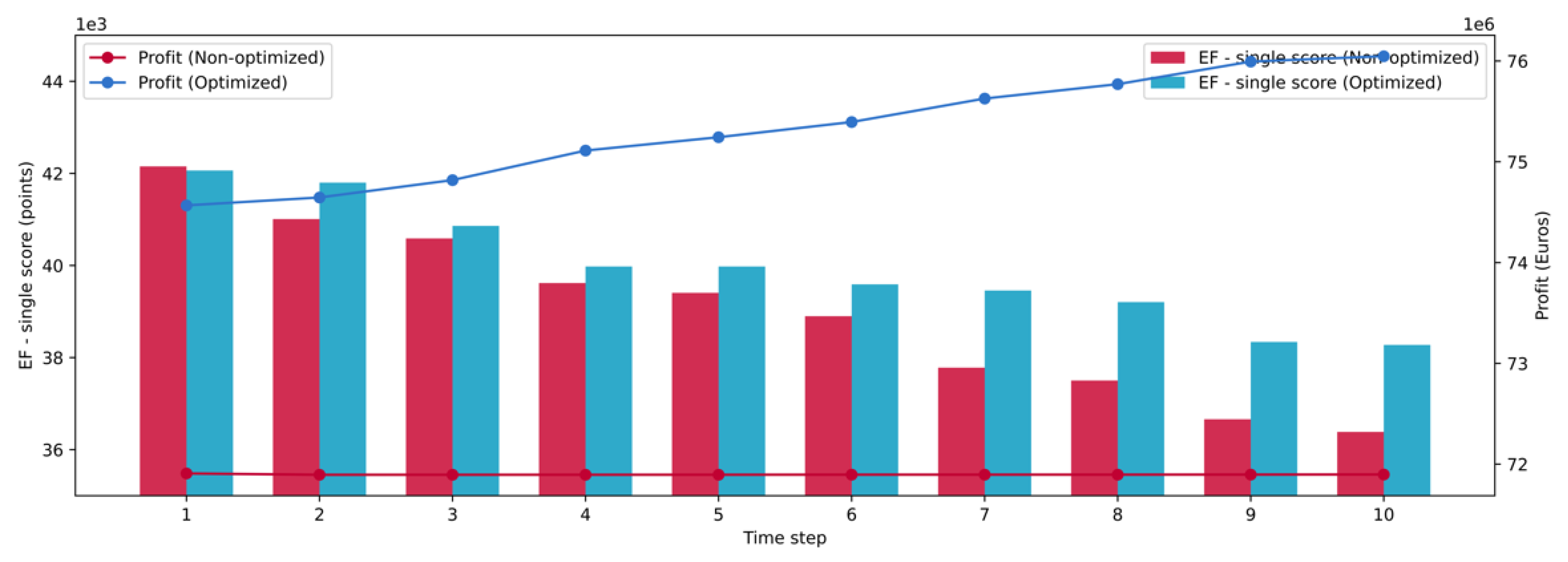
Figure 2. LSU / ha change for different cases.

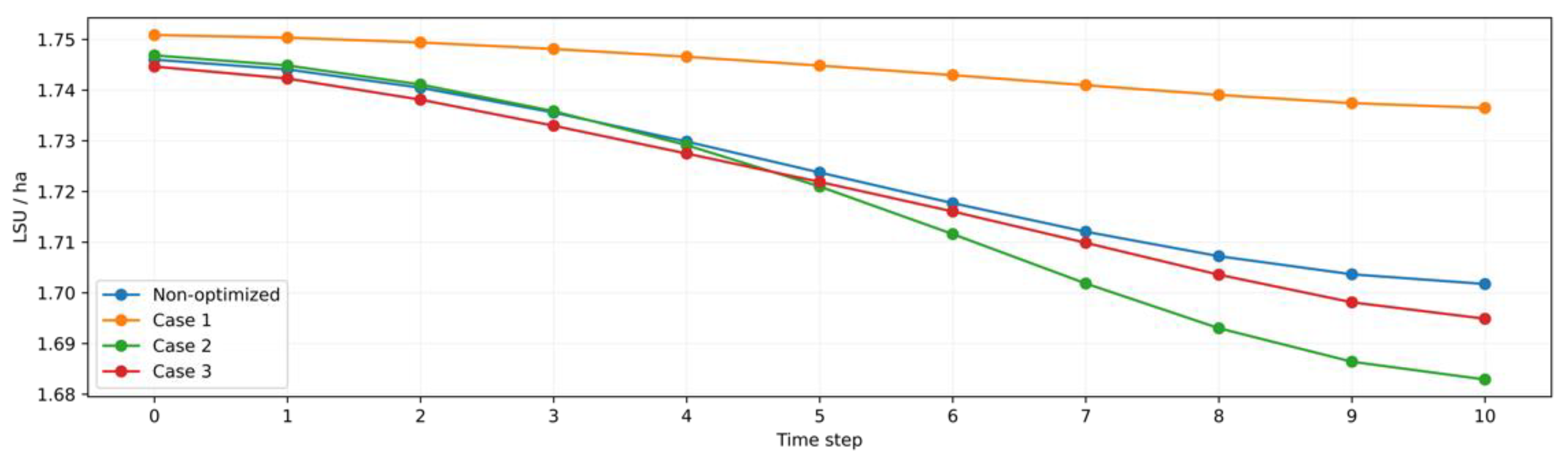
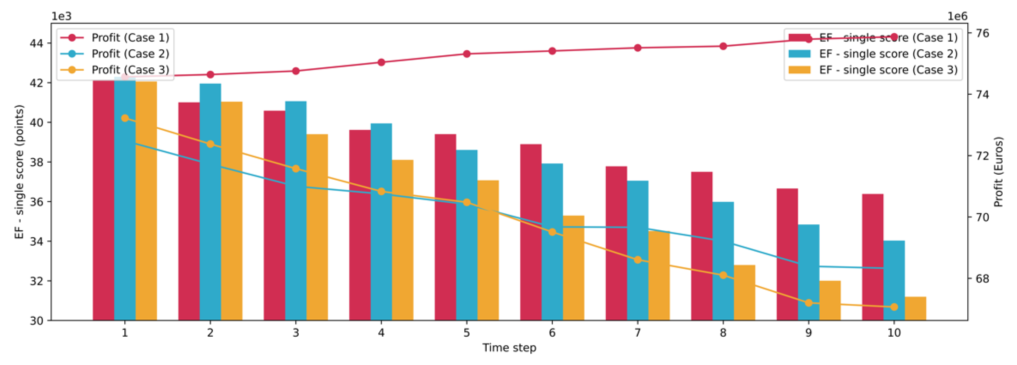
Figure 3 shows a comparison of the EF single scores for each case. The aggregated impacts and profits at the country level reveal that there is an obvious trade-off between environmental and economic sustainability. Although a 25% reduction in total emissions is attainable if farming operations are affected by environmental concerns, this results in an 8% decrease in profitability over ten years. As shown in Figure 2, the average stocking density drops to 1.6 LSU/ha, but the subsidy "Extensification of permanent grassland" necessitates a far lower stocking rate. Most farms fall short of this target because the quantity of subsidies supplied is insufficient to allow farmers to make more culling decisions. Nevertheless, as shown, if a mathematical optimization is put in place, around 9% of EF single score reduction can still be achieved while making 5.5% more profit. Nonetheless, as seen in Figure 1, if mathematical optimization is used, a 9% decrease in EF single score may still be achieved while increasing profit by 5.5%.

Figure 3. Comparison of EF single scores based on each optimization case.

Figure 3. Comparison of EF single scores based on each optimization case.

3.2. Farm-Level Results

Because agricultural activities, agent choices, and optimization occur at the farm level, it is natural to focus on farm level results for the simulated scenarios. As a result, we used ground truth data to initialize several farms. For example, we choose one of those farms whose parameters, such as location, size, and animal count, are known, and in this section we will illustrate the outcomes of the simulations for this specific farm. The other farms' behavior is fairly similar. Table 6 lists the farm's properties. Some characteristics, like as GC and livestock count, adjust throughout the simulation. For those attributes, the initial, minimum, mean, and maximum values are reported. The GC, degree centrality of the farm in the network, and crop rotation scheme are allocated using a random distribution.

Table 6. Properties of the farm selected as an example. It is a dairy farm located around the center of the Grand Duchy of Luxembourg. Farm class and rotation scheme codes are explained in [18].

Attribute		Value
Farm class		G
Degree centrality		2
Green Consciousness (GC)	Initial:	0.44
	Min:	0.44
	Mean:	0.47
	Max:	0.51
Number of fields		36
Number of arable fields		10
Size of pastureland (ha)		22.00
Size of arable land (ha)		69.50
Total size of UAA (ha)		91.51
Number of Livestock	Initial:	122
	Min:	105
	Mean:	114
	Max:	125
Organic		No
Rotation Scheme		MLC

Table 6. Properties of the farm selected as an example. It is a dairy farm located around the center of the Grand Duchy of Luxembourg. Farm class and rotation scheme codes are explained in [18].

Attribute		Value
Farm class		G
Degree centrality		2
Green Consciousness (GC)	Initial:	0.44
	Min:	0.44
	Mean:	0.47
	Max:	0.51
Number of fields		36
Number of arable fields		10
Size of pastureland (ha)		22.00
Size of arable land (ha)		69.50
Total size of UAA (ha)		91.51
Number of Livestock	Initial:	122
	Min:	105
	Mean:	114
	Max:	125
Organic		No
Rotation Scheme		MLC

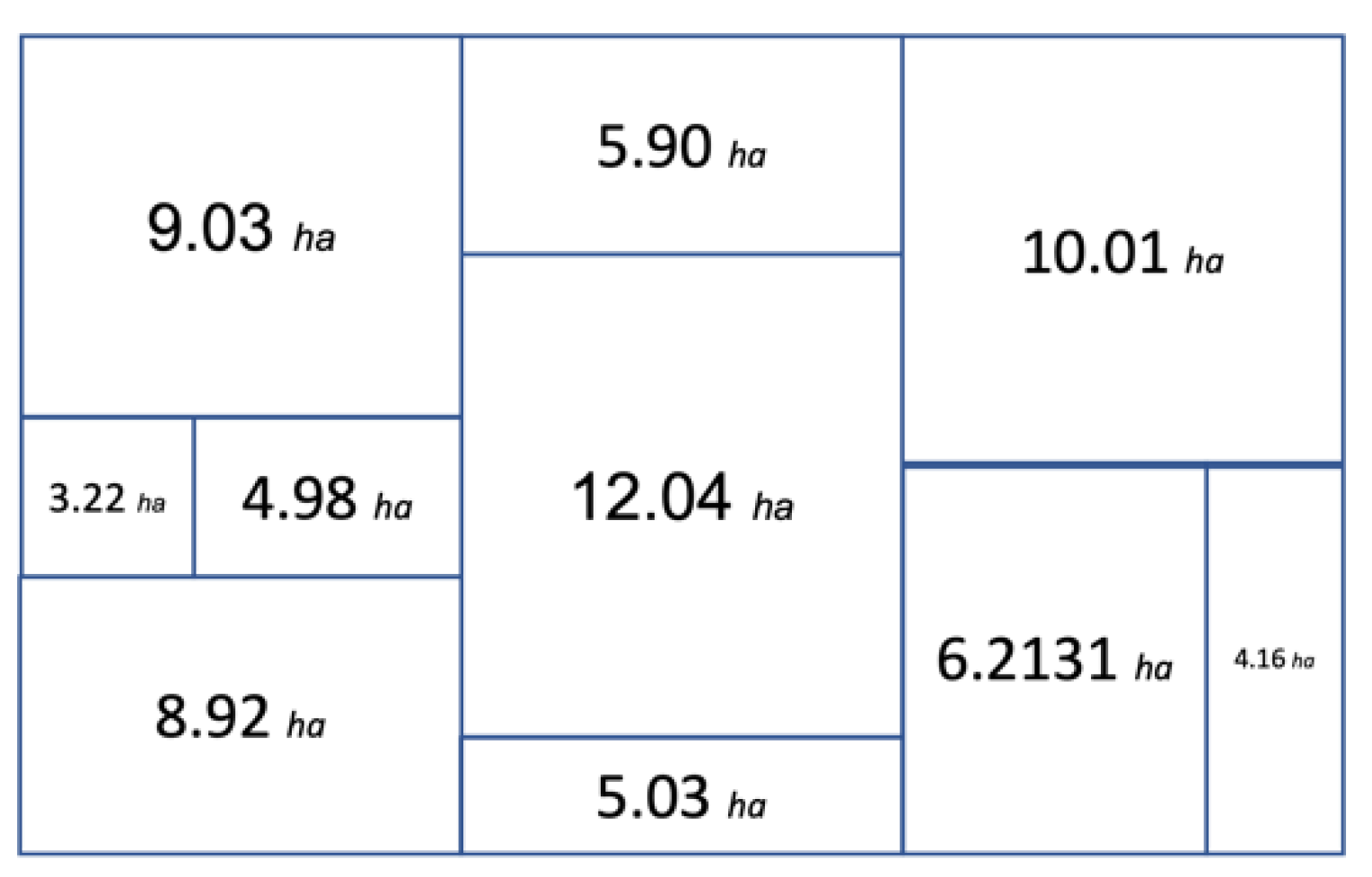
To maintain the privacy of a farm's outer geographical boundaries while preserving the inner boundaries (i.e., field boundaries) and relative sizes, a treemap representation of the UAAs was applied (Marvuglia et al., 2022). Figure 4 depicts the treemap representation of the chosen farm.

Figure 4. Treemap visualization of the chosen farm’s UAAs. The sizes of the fields used in the simulator are shown in the map.

Figure 4. Treemap visualization of the chosen farm’s UAAs. The sizes of the fields used in the simulator are shown in the map.

This representation is also used in Error! Reference source not found., Figure 8 and Figure 11, where, the treemaps depict the progress of agricultural plantations during ten years of simulation from the top left (step 1) to the bottom right (step 10) corner. To retain the geolocation of fields on the specified farm, the treemap representation shows the positions of the fields and crops. Observing these figures, one can identify which crops were prevalent on the fields, knowing that transitions from one crop to another in a specific UUA can occur at any time step, as long as crop rotation, seeding and harvesting months, and optimization objectives and constraints permit. Crop rotation constraints compel farmers to select only a few crops. As a result, the environmental impact and economic profitability of crop selections are the same in each case. However, in Case 1 (Error! Reference source not found.), potatoes are chosen more frequently than other L crops, owing to the greater market value of potatoes in comparison to other crops. Because of its significance as animal feed, maize is a crop that practically every farm cultivates and includes into its crop rotation strategy.

Figure 6, Figure 9 and Figure 12 depict the progression of the EF impact scores during the simulation steps for Cases 1, Case 2, and Case 3, respectively. The other choice variable in the optimization problem, i.e., the quantity of cattle to be retained on the farm (NL), has the greatest influence on the environmental impact generated.

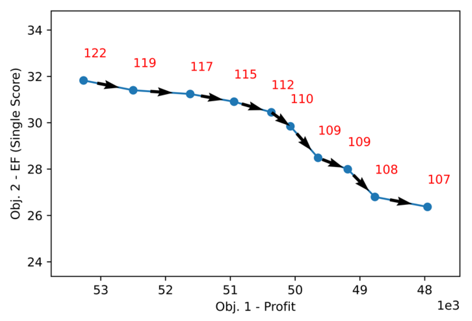
Figure 7, Figure 10 and Figure 13 (respectively for Cases 1, Case 2 and Case 3) indicate the change in cattle at each time step when associated optimization targets are taken into account. They also show the associated earnings (in k€ on the x-axis) and environmental impacts. The arrows reflect the advancement of the simulation steps and each point on the graph represents one year. Since Case 1 merely optimizes profit, farmers prefer to slaughter fewer animals, resulting in a 7% reduction in EF single score (Figure 7). However, profits remain almost unchanged over the last ten years. In Case 2, the optimization problem takes the EF climate change score into account, and a 19% decrease in climate change impact may be obtained (Figure 9), but this comes at a cost, as more culling choices are taken than in the baseline scenario. In this scenario, the NL has lowered by 15% after the environmental component was introduced to the objective function. Finally, when compared to Case 2, Case 3 shows a 12% fall in NL (Figure 12), which may be explained by the fact that livestock agricultural operations contribute significantly more to the EF climate change score than to the EF single score. Therefore, the culling decisions can be taken more easily in Case 2 than in Case 3.

Figure 5. Crop rotations for a pilot farm with the scheme MLC (Case 1).

Figure 5. Crop rotations for a pilot farm with the scheme MLC (Case 1).

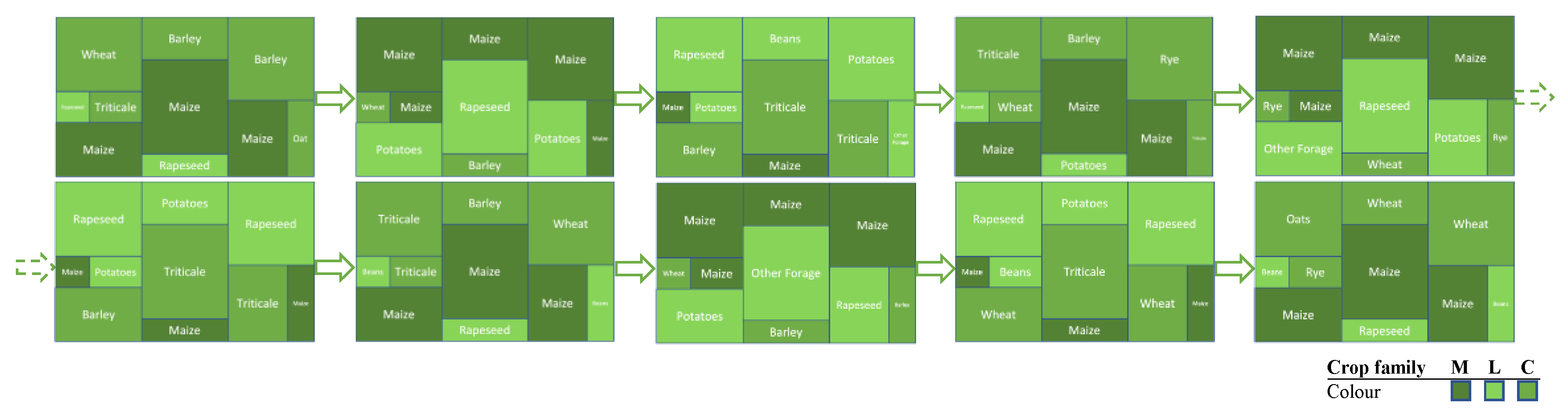
Figure 6. Evolution of single score and climate change impacts for Case 1 along the simulation steps.

Figure 6. Evolution of single score and climate change impacts for Case 1 along the simulation steps.

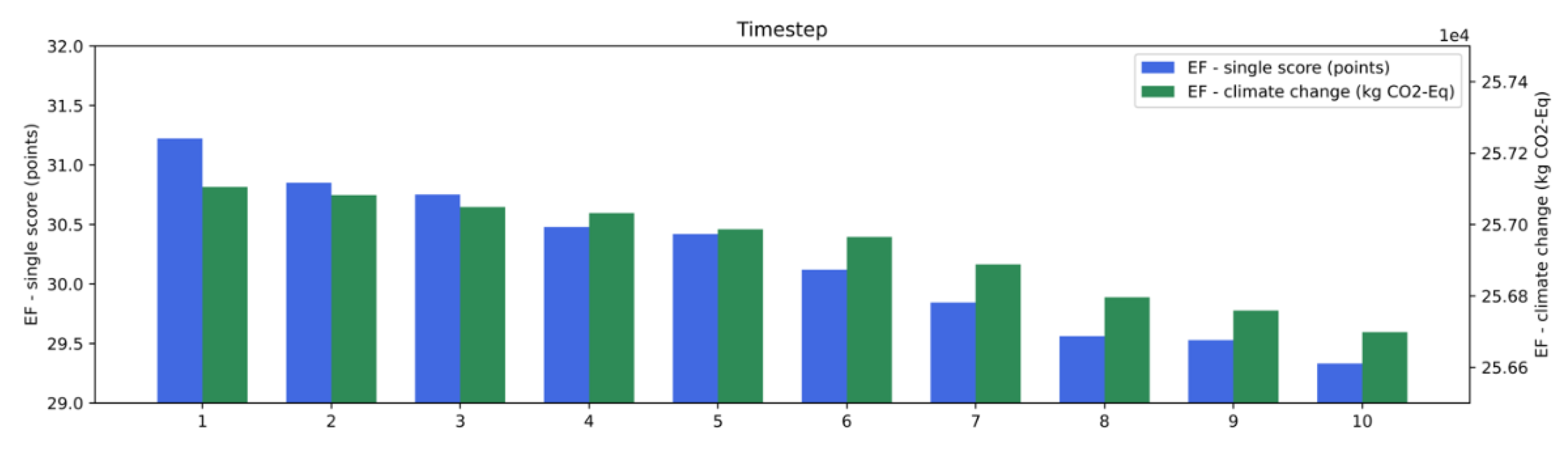
Figure 7. Change of number of livestock (in red), profit and environmental impact expressed as EF single score, in Case 1, for the selected farm.

Figure 7. Change of number of livestock (in red), profit and environmental impact expressed as EF single score, in Case 1, for the selected farm.

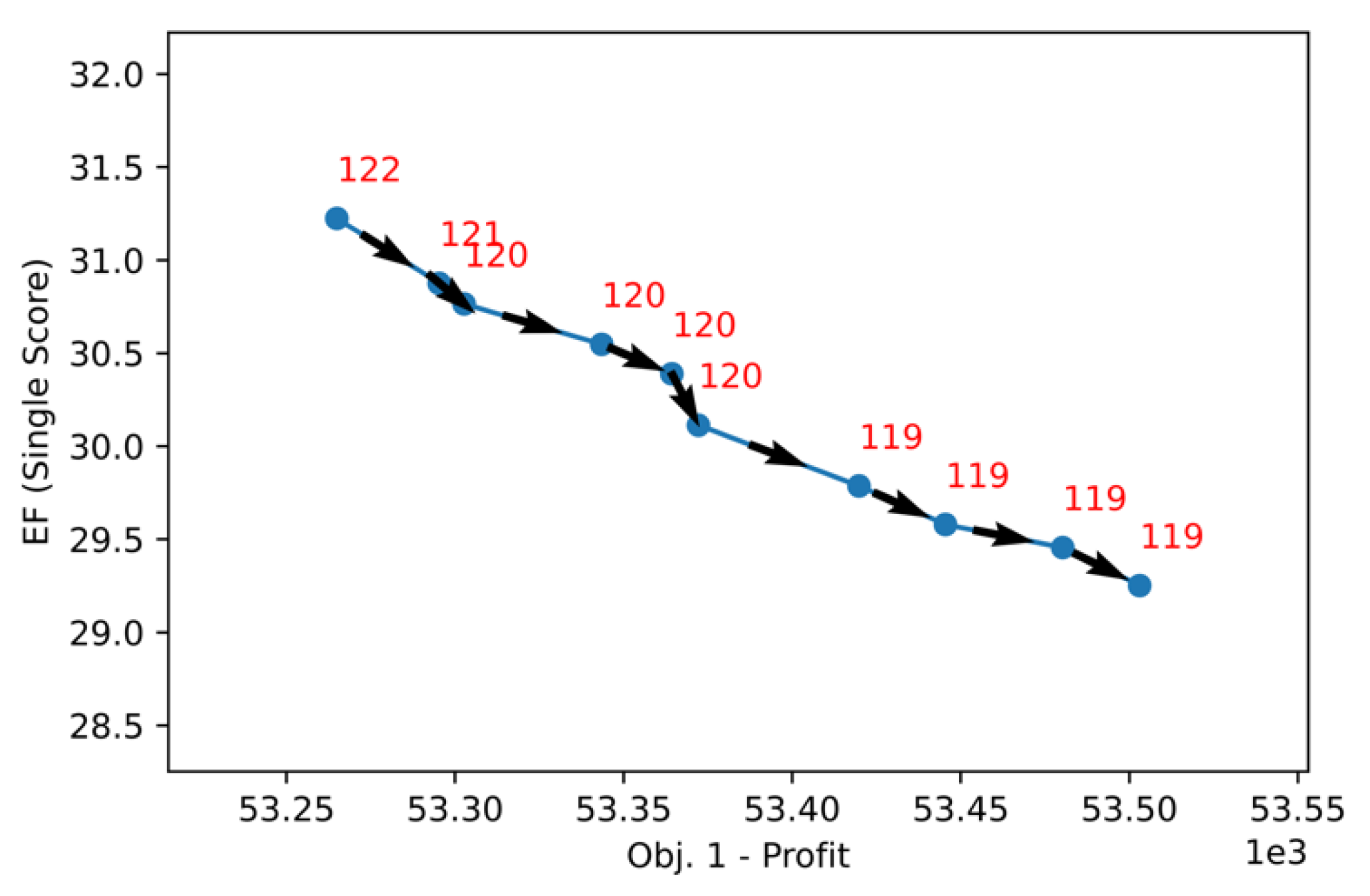
Figure 8. Crop rotations for a pilot farm with the scheme MLC (Case 2).

Figure 8. Crop rotations for a pilot farm with the scheme MLC (Case 2).

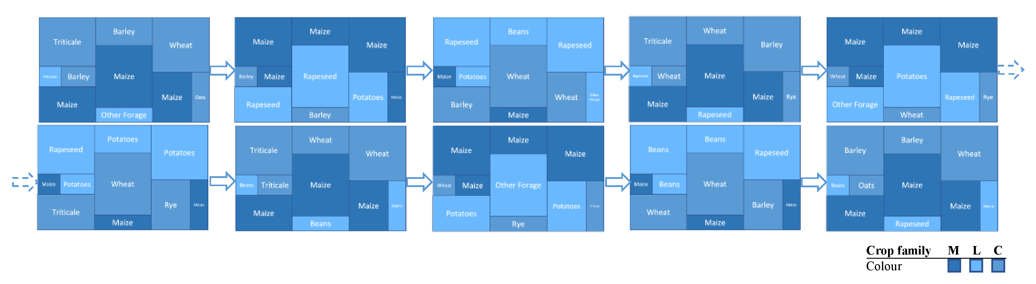
Figure 9. Evolution of single score and climate change impacts for Case 2 along the simulation steps.

Figure 9. Evolution of single score and climate change impacts for Case 2 along the simulation steps.

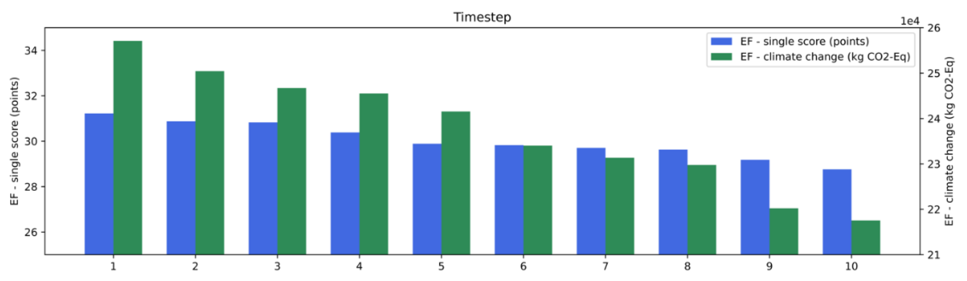
Figure 10. Change of number of livestock (in red), environmental impact expressed as EF Climate Change score, in Case 1, for the selected farm. Note: the x-axis is reversed.

Figure 10. Change of number of livestock (in red), environmental impact expressed as EF Climate Change score, in Case 1, for the selected farm. Note: the x-axis is reversed.

Figure 11. Crop rotations for a pilot farm with the scheme MLC (Case 3).

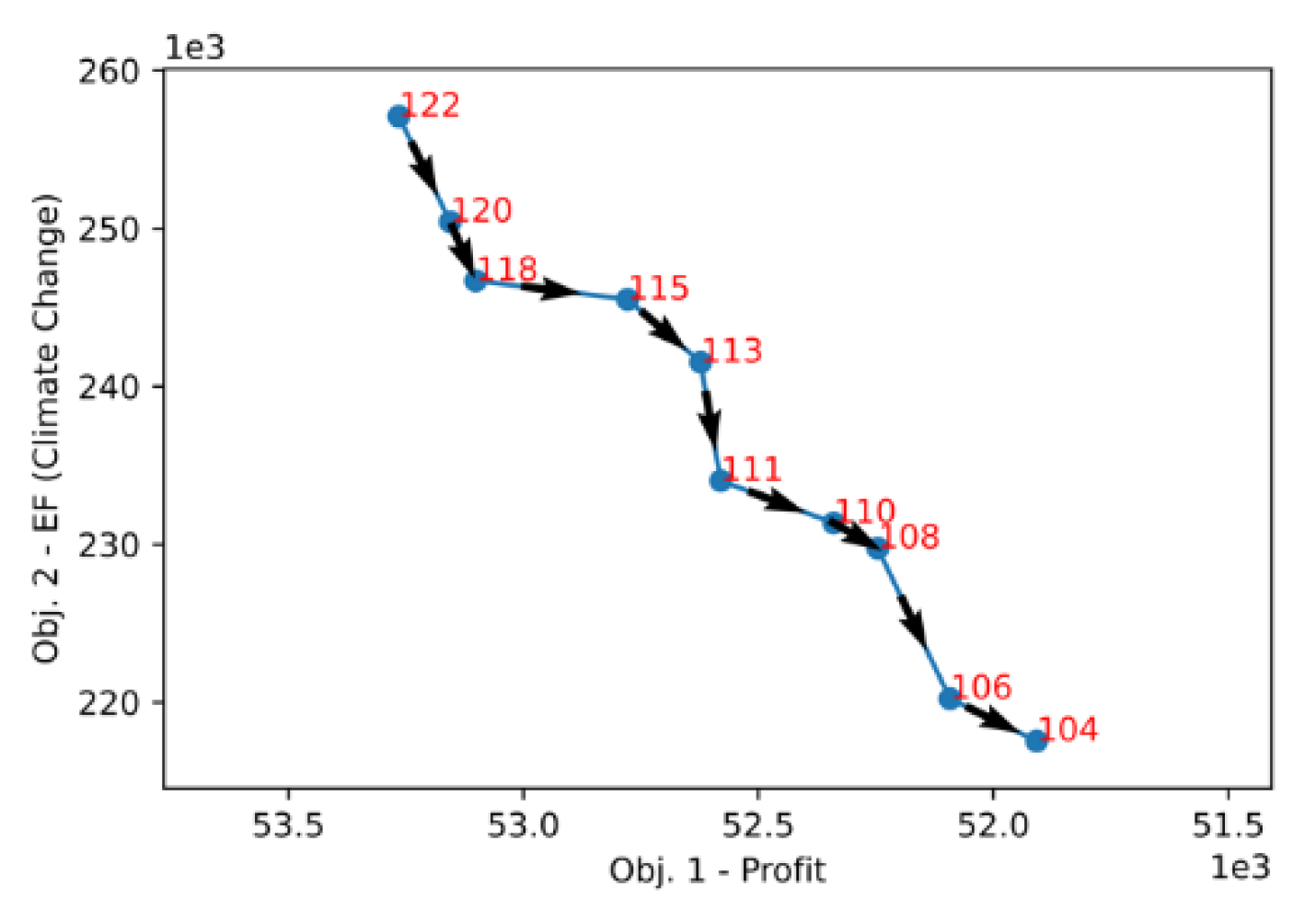
Figure 11. Crop rotations for a pilot farm with the scheme MLC (Case 3).

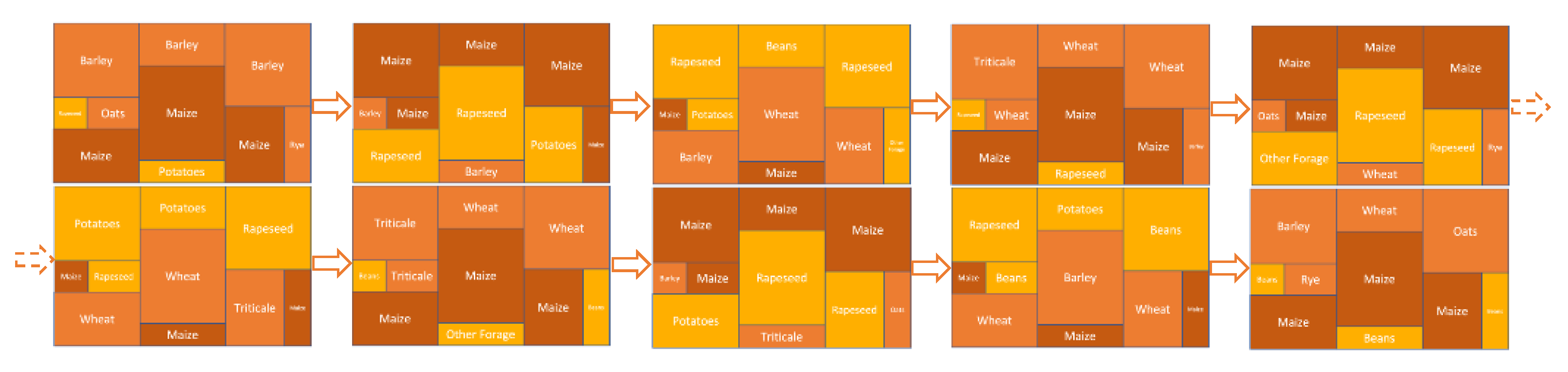
Figure 12. Evolution of single score and climate change impacts for Case 3 along the simulation steps.

Figure 12. Evolution of single score and climate change impacts for Case 3 along the simulation steps.

Figure 13. Change of number of livestock (in red), environmental impact expressed as EF single score, in Case 3, for the selected farm.

Figure 13. Change of number of livestock (in red), environmental impact expressed as EF single score, in Case 3, for the selected farm.

5. Conclusions

This paper describes a coupled ABM-LCA model for agricultural livestock operations that includes MOO under economic and environmental constraints. The potential of different modelling strategies to decrease the environmental impacts of farms' practices was assessed based on several environmental impact indicators.

The article's main original contributions consist in:

• A unique multi-stage optimization model for efficient farm management that takes crop and livestock operations into account.
• An agricultural management system that optimizes decision-making based on subsidies to minimize environmental impacts.

To examine the impact of including optimization in our model, we first compared the baseline scenario's non-optimized instantiation (i.e. a version without mathematical optimization) to the optimized version. The baseline scenario only contains decisions dealing with financial actions in optimized and non-optimized variants. We discovered that the version with optimization in place performs better in terms of profit generation, with a 5.5% rise in revenue whereas the prior version of our model showed no change in profit over 10 years.

After determining that the optimization model produces superior outcomes for the objectives under consideration, we concentrated on many scenarios that optimize decisions based on economic, environmental, or both objectives. In Case 1, the optimization model just examines agricultural profitability, with no environmental goals in mind. Cases 2 and 3 additionally include an environmental goal in the decision function to minimize. The former minimizes EF climate change scores, whereas the latter targets EF single scores utilizing all 16 categories listed in the S4 file Cases 2 and 3 suggest a greater fall in stocking rates (3.5% and 2.3%, respectively) than Case 1, which may be explained by the environmental effect of cattle production operations. These two scenarios take into account the environmental objective and farmers who are "green conscious" enough to make decisions to lessen the environmental impact of their activity.

Figure 7 and Figure 10 demonstrate a pattern of decreasing stocking rate on the example farm mentioned in Section 0. In Cases 2 and 3, the number of livestock is reduced by 15% and 12%, respectively.

In conclusion, even though the cases we evaluated are by no means exhaustive, they highlight the general utility and efficacy of farm optimization as well as demonstrating the compromise between environmental and economic objectives. Maximizing profit mainly means keeping a higher stocking rate and relatively stable income (besides changes in market conditions, which are not considered in our simulations), but this does not allow to make emissions decrease. In fact, the results of our simulations show that, although reducing overall impacts by 25% is possible if an optimization model is put in place to steer farmers’ decisions, this brings an inevitable reduction in economic profitability over ten years (about 8%) in Case 3. Obviously, this consideration holds true (besides the limits of the uncertainty that such a complex hybrid model bears, and which are discussed in the S4 file) without considering other complementary investments by the farmers or institutional economic incentives and income support for non-mandatory actions that may seem necessary to compensate for the economic losses.

However, on this last point we need to spend a word of caution, since, as it was observed by [49], if on one hand there is evidence that farmers prefer voluntary over mandatory measures (especially if mandatory instruments are overly complex or inflexible), on the other hand crowding out (and only to a lesser extent also crowding in) has been observed when economic incentives are used to encourage the voluntary instruments [50]. Therefore, from a policy perspective, a delicate equilibrium should be found between requesting compliance with mandatory environmental regulations and decreasing unconditional income support. In their accurate analysis, [49] point out that, from an economic standpoint, the unilateral adoption of mandatory compliance with more stringent environmental regulations without monetary compensation, “can hamper the competitiveness of agriculture and may also lead to dissatisfaction and protest on the side of the farmers”. Voluntary instruments, on the other hand, may strengthen farmers' motivation to safeguard the environment (i.e., their green awareness) through education more than obligatory instruments [51]. Concerning this last point though, the short survey presented in the S4 file, which was distributed to a small number of pilot farms (not statistically significant), shows that some farmers in Luxembourg have the perception that they are already doing enough efforts to protect the environment (and therefore implicitly considering that no further effort should be requested from them), while others are not fully aware of the important impacts that agriculture and farming generate on the planet. Obviously, the sample is too small (0.5% of the farmers’ population) to generalize any conclusion, but at least we can use it to confirm some of the considerations that can be very useful in the design of an agricultural ABM, such as the important role played by family members in the decision-taking process of the farmers, or the popularity of solar panel installations as complementary investment that combines economic return with environmental protection.

References

- Eurostat. Available online: https://ec.europa.eu/eurostat/data/database (accessed on 8 February 2022).
- Twine, R. Emissions from Animal Agriculture—16.5% Is the New Minimum Figure. Sustainability 2021, 13, 6276. [Google Scholar] [CrossRef]
- Schreinemachers, P.; Berger, T. An Agent-Based Simulation Model of Human–Environment Interactions in Agricultural Systems. Environmental Modelling & Software 2011, 26, 845–859. [Google Scholar] [CrossRef]
- Ferber, J.; Weiss, G. Multi-Agent Systems: An Introduction to Distributed Artificial Intelligence; Addison-wesley Reading, 1999; Vol. 1;
- An, L. Modeling Human Decisions in Coupled Human and Natural Systems: Review of Agent-Based Models. Ecological Modelling 2012, 229, 25–36. [Google Scholar] [CrossRef]
- Hare, M.; Deadman, P. Further towards a Taxonomy of Agent-Based Simulation Models in Environmental Management. Mathematics and Computers in Simulation 2004, 64, 25–40. [Google Scholar] [CrossRef]
- Baustert, P.; Navarrete Gutiérrez, T.; Gibon, T.; Chion, L.; Ma, T.-Y.; Mariante, G.L.; Klein, S.; Gerber, P.; Benetto, E. Coupling Activity-Based Modeling and Life Cycle Assessment—A Proof-of-Concept Study on Cross-Border Commuting in Luxembourg. Sustainability 2019, 11, 4067. [Google Scholar] [CrossRef]
- Gaud, N.; Galland, S.; Gechter, F.; Hilaire, V.; Koukam, A. Holonic Multilevel Simulation of Complex Systems: Application to Real-Time Pedestrians Simulation in Virtual Urban Environment. Simulation Modelling Practice and Theory 2008, 16, 1659–1676. [Google Scholar] [CrossRef]
- Gilbert, N. Agent-Based Models; Sage Publications, 2019; Vol. 153;
- Grimm, V.; Railsback, S.F. Individual-Based Modeling and Ecology; Princeton University Press, 2013; ISBN 978-1-4008-5062-4.
- Heath, B.; Hill, R.; Ciarallo, F. A Survey of Agent-Based Modeling Practices (January 1998 to July 2008). Journal of Artificial Societies and Social Simulation 2009, 12, 9. [Google Scholar]
- Heckbert, S.; Baynes, T.; Reeson, A. Agent-Based Modeling in Ecological Economics. Annals of the New York Academy of Sciences 2010, 1185, 39–53. [Google Scholar] [CrossRef] [PubMed]
- Micolier, A.; Taillandier, F.; Taillandier, P.; Bos, F. Li-BIM, an Agent-Based Approach to Simulate Occupant-Building Interaction from the Building-Information Modelling. Engineering Applications of Artificial Intelligence 2019, 82, 44–59. [Google Scholar] [CrossRef]
- Teglio, A. From Agent-Based Models to Artificial Economies. Ph.D. Thesis, Universitat Jaume I, 2011.
- Wu, S.R.; Li, X.; Apul, D.; Breeze, V.; Tang, Y.; Fan, Y.; Chen, J. Agent-Based Modeling of Temporal and Spatial Dynamics in Life Cycle Sustainability Assessment. Journal of Industrial Ecology 2017, 21, 1507–1521. [Google Scholar] [CrossRef]
- Marvuglia, A.; Bayram, A.; Baustert, P.; Gutiérrez, T.N.; Igos, E. Agent-Based Modelling to Simulate Farmers’ Sustainable Decisions: Farmers’ Interaction and Resulting Green Consciousness Evolution. Journal of Cleaner Production 2022, 332, 129847. [Google Scholar] [CrossRef]
- Life Cycle Assessment: Theory and Practice; Hauschild, M.Z., Rosenbaum, R.K., Olsen, S.I., Eds.; Springer International Publishing, 2017; ISBN 978-3-319-56475-3.
- Bayram, A.; Marvuglia, A.; Gutierrez, T.N.; Weis, J.-P.; Conter, G.; Zimmer, S. Sustainable Farming Strategies for Mixed Crop-Livestock Farms in Luxembourg Simulated with a Hybrid Agent-Based and Life-Cycle Assessment Model. Journal of Cleaner Production 2023, 386, 135759. [Google Scholar] [CrossRef]
- Repar, N.; Jan, P.; Dux, D.; Nemecek, T.; Doluschitz, R. Implementing Farm-Level Environmental Sustainability in Environmental Performance Indicators: A Combined Global-Local Approach. Journal of Cleaner Production 2017, 140, 692–704. [Google Scholar] [CrossRef]
- Chandrasekaran, M.; Ranganathan, R. Modelling and Optimisation of Indian Traditional Agriculture Supply Chain to Reduce Post-Harvest Loss and CO2 Emission. Industrial Management & Data Systems 2017, 117, 1817–1841. [Google Scholar] [CrossRef]
- He, P.; Li, J.; Wang, X. Wheat Harvest Schedule Model for Agricultural Machinery Cooperatives Considering Fragmental Farmlands. Computers and Electronics in Agriculture 2018, 145, 226–234. [Google Scholar] [CrossRef]
- Carravilla, M.A.; Oliveira, J.F. Operations Research in Agriculture: Better Decisions for a Scarce and Uncertain World. 2013.
- Xie, Y.L.; Xia, D.X.; Ji, L.; Huang, G.H. An Inexact Stochastic-Fuzzy Optimization Model for Agricultural Water Allocation and Land Resources Utilization Management under Considering Effective Rainfall. Ecological Indicators 2018, 92, 301–311. [Google Scholar] [CrossRef]
- Yuanyuan, Z. Research on multi-objective planning model for agricultural pollution, environmental regulation and economic development. Arch. Latinoam. Nutr. 2020, 70, 423–433. [Google Scholar]
- Huber, R.; Bakker, M.; Balmann, A.; Berger, T.; Bithell, M.; Brown, C.; Grêt-Regamey, A.; Xiong, H.; Le, Q.B.; Mack, G.; et al. Representation of Decision-Making in European Agricultural Agent-Based Models. Agricultural Systems 2018, 167, 143–160. [Google Scholar] [CrossRef]
- Kremmydas, D.; Athanasiadis, I.N.; Rozakis, S. A Review of Agent Based Modeling for Agricultural Policy Evaluation. Agricultural Systems 2018, 164, 95–106. [Google Scholar] [CrossRef]
- Grimm, V.; Railsback, S.F.; Vincenot, C.E.; Berger, U.; Gallagher, C.; DeAngelis, D.L.; Edmonds, B.; Ge, J.; Giske, J.; Groeneveld, J.; et al. The ODD Protocol for Describing Agent-Based and Other Simulation Models: A Second Update to Improve Clarity, Replication, and Structural Realism. Journal of Artificial Societies and Social Simulation 2020, 23, 7. [Google Scholar] [CrossRef]
- Davoud Heidari, M.; Turner, I.; Ardestani-Jaafari, A.; Pelletier, N. Operations Research for Environmental Assessment of Crop-Livestock Production Systems. Agricultural Systems 2021, 193, 103208. [Google Scholar] [CrossRef]
- Moher, D.; Liberati, A.; Tetzlaff, J.; Altman, D.G.; Antes, G.; Atkins, D.; Barbour, V.; Barrowman, N.; Berlin, J.A.; Clark, J.; et al. Preferred Reporting Items for Systematic Reviews and Meta-Analyses: The PRISMA Statement. PLOS Medicine 2009, 6, e1000097. [Google Scholar] [CrossRef] [PubMed]
- Page, M.J.; McKenzie, J.E.; Bossuyt, P.M.; Boutron, I.; Hoffmann, T.C.; Mulrow, C.D.; Shamseer, L.; Tetzlaff, J.M.; Akl, E.A.; Brennan, S.E.; et al. The PRISMA 2020 Statement: An Updated Guideline for Reporting Systematic Reviews. Systematic Reviews 2021, 10, 89. [Google Scholar] [CrossRef] [PubMed]
- Galán-Martín, Á.; Vaskan, P.; Antón, A.; Esteller, L.J.; Guillén-Gosálbez, G. Multi-Objective Optimization of Rainfed and Irrigated Agricultural Areas Considering Production and Environmental Criteria: A Case Study of Wheat Production in Spain. Journal of Cleaner Production 2017, 140, 816–830. [Google Scholar] [CrossRef]
- Gebrezgabher, S.A.; Meuwissen, M.P.M.; Oude Lansink, A.G.J.M. A Multiple Criteria Decision Making Approach to Manure Management Systems in the Netherlands. European Journal of Operational Research 2014, 232, 643–653. [Google Scholar] [CrossRef]
- Udias, A.; Pastori, M.; Dondeynaz, C.; Carmona Moreno, C.; Ali, A.; Cattaneo, L.; Cano, J. A Decision Support Tool to Enhance Agricultural Growth in the Mékrou River Basin (West Africa). Computers and Electronics in Agriculture 2018, 154, 467–481. [Google Scholar] [CrossRef] [PubMed]
- Holland, J.H. Adaptation in Natural and Artificial Systems: An Introductory Analysis with Applications to Biology, Control, and Artificial Intelligence; MIT Press, 1992; ISBN 978-0-262-58111-0.
- Deb, K.; Pratap, A.; Agarwal, S.; Meyarivan, T. A Fast and Elitist Multiobjective Genetic Algorithm: NSGA-II. IEEE Trans. Evol. Computat. 2002, 6, 182–197. [Google Scholar] [CrossRef]
- Yusoff, Y.; Ngadiman, M.S.; Zain, A.M. Overview of NSGA-II for Optimizing Machining Process Parameters. Procedia Engineering 2011, 15, 3978–3983. [Google Scholar] [CrossRef]
- Maiyar, L.M.; Thakkar, J.J. Environmentally Conscious Logistics Planning for Food Grain Industry Considering Wastages Employing Multi Objective Hybrid Particle Swarm Optimization. Transportation Research Part E: Logistics and Transportation Review 2019, 127, 220–248. [Google Scholar] [CrossRef]
- Pishgar-Komleh, S.H.; Akram, A.; Keyhani, A.; Sefeedpari, P.; Shine, P.; Brandao, M. Integration of Life Cycle Assessment, Artificial Neural Networks, and Metaheuristic Optimization Algorithms for Optimization of Tomato-Based Cropping Systems in Iran. Int J Life Cycle Assess 2020, 25, 620–632. [Google Scholar] [CrossRef]
- Pastori, M.; Udías, A.; Bouraoui, F.; Bidoglio, G. Multi-Objective Approach to Evaluate the Economic and Environmental Impacts of Alternative Water and Nutrient Management Strategies in Africa. Journal of Environmental Informatics 2017, 29, 16–28. [Google Scholar] [CrossRef]
- Deb, K.; Jain, H. An Evolutionary Many-Objective Optimization Algorithm Using Reference-Point-Based Nondominated Sorting Approach, Part I: Solving Problems With Box Constraints. IEEE Transactions on Evolutionary Computation 2014, 18, 577–601. [Google Scholar] [CrossRef]
- Saouter, E.; Biganzoli, F.; Ceriani, L.; Versteeg, D.; Crenna, E.; Zampori, L.; Sala, S.; Pant, R. Environmental Footprint: Update of Life Cycle Impact Assessment Methods – Ecotoxicity Freshwater, Human Toxicity Cancer, and Non-Cancer. Available online: https://publicationstest.jrc.cec.eu.int/repository/handle/JRC114227 (accessed on 7 March 2023).
- Tedde, A.; Grelet, C.; Ho, P.N.; Pryce, J.E.; Hailemariam, D.; Wang, Z.; Plastow, G.; Gengler, N.; Brostaux, Y.; Froidmont, E.; et al. Validation of Dairy Cow Bodyweight Prediction Using Traits Easily Recorded by Dairy Herd Improvement Organizations and Its Potential Improvement Using Feature Selection Algorithms. Animals 2021, 11, 1288. [Google Scholar] [CrossRef] [PubMed]
- Hadka, D. MOEA Framework-a Free and Open Source Java Framework for Multiobjective Optimization 2012.
- Arnold, K.; Gosling, J.; Holmes, D. The Java Programming Language; Addison Wesley Professional, 2005.
- Deb, K.; Agrawal, R.B.; et al. Simulated Binary Crossover for Continuous Search Space. Complex systems 1995, 9, 115–148. [Google Scholar]
- Kita, H.; Ono, I.; Kobayashi, S. Multi-Parental Extension of the Unimodal Normal Distribution Crossover for Real-Coded Genetic Algorithms. In Proceedings of the Proceedings of the 1999 Congress on Evolutionary Computation-CEC99 (Cat. No. 99TH8406); July 1999; Vol. 2, pp. 1581-1588 Vol. 2.
- Gouvernement du Luxembourg Règlement Grand-Ducal Du 24 Novembre 2000 Concernant l’utilisation de Fertilisants Azotés Dans l’agriculture. J. Off. Grand-Duché Luxembourg <bold>2000</bold>, A n.124.
- SER Durchführung in Luxemburg der Cross Compliance im Rahmen der gemeinsamen Agrarpolitik. Available online: http://agriculture.public.lu/de/publications/weinbau/prime/crosscompliance.html (accessed on 15 February 2022).
- Barreiro-Hurle, J.; Dessart, F.J.; Rommel, J.; Czajkowski, M.; Espinosa-Goded, M.; Rodriguez-Entrena, M.; Thomas, F.; Zagorska, K. Willing or Complying? The Delicate Interplay between Voluntary and Mandatory Interventions to Promote Farmers’ Environmental Behavior. Food Policy 2023, 120, 102481. [Google Scholar] [CrossRef]
- Rode, J.; Gómez-Baggethun, E.; Krause, T. Motivation Crowding by Economic Incentives in Conservation Policy: A Review of the Empirical Evidence. Ecological Economics 2015, 117, 270–282. [Google Scholar] [CrossRef]
- Bosch, D.J.; Cook, Z.L.; Fuglie, K.O. Voluntary versus Mandatory Agricultural Policies to Protect Water Quality: Adoption of Nitrogen Testing in Nebraska. Applied Economic Perspectives and Policy 1995, 17, 13–24. [Google Scholar] [CrossRef]